Distributed transient frequency control in power networks

Abstract

Modern power networks face increasing challenges in controlling their transient frequency behavior at acceptable levels due to low inertia and highly-dynamic units. This paper presents a distributed control strategy regulated on a subset of buses in a power network to maintain their transient frequencies in safe regions while preserving asymptotic stability of the overall system. Building on Lyapunov stability and set invariance theory, we formulate the transient frequency requirement and the asymptotic stability requirement as two separate constraints for the control input. Hereby, for each bus of interest, we synthesize a controller satisfying both constraints simultaneously. The controller is distributed and Lipschitz, guaranteeing the existence and uniqueness of the trajectories of the closed-loop system. Simulations on the IEEE 39-bus power network illustrate the results.

I Introduction

To avoid a power system from running underfrequency or to help the network recover from it, load shedding and curtailment are commonly employed to balance supply and demand. However, due to inertia, it takes some time for the energy resources to re-enter a safe frequency region until the power network eventually converges to steady state. Hence, during transients, generators are still in danger of reaching their frequency limits and being tripped, which may in turn cause blackouts. Therefore, there is a need to analyze the transient behavior of power networks and design controllers that ensure the safe evolution of the system.

Literature review

Transient stability refers to the ability of power networks to maintain synchronism after being subjected to a disturbance, see e.g. [1]. The works [2, 3, 4] provide conditions to ensure synchronicity and investigate their relationship with the topology of the power network. However, even if network synchronism holds, system transient trajectory may enter unsafe regions, e.g., transient frequency may violate individual generator’s frequency limits, causing generator failure and leading to blackouts [5]. Hence, various techniques have been proposed to improve transient behavior. These include resource re-dispatch with transient stability constraints [6, 7]; the use of power system stabilizers to damp out low frequency inter-machine oscillations [8], and placing virtual inertia in power networks to mitigate transient effects [9, 10]. While these approaches have a qualitative effect on transient behavior, they do not offer strict guarantees as to whether the transient frequency stays within a specific region. Furthermore, the approach in [9] requires a priori knowledge of the time evolution of the disturbance trajectories and an estimation of the transient overshoot. Alternative approaches rely on the idea of identifying the disturbances that may cause undesirable transient behaviors using forward and backward reachability analysis, see e.g., [11, 12] and our previous work [13]. The general lack of works that provide tools for transient frequency control motivates us here to design feedback controllers for the generators that guarantee simultaneously the stability of the power network and the desired transient frequency behavior. Our design is inspired by the controller-design approach to safety-constrained systems taken in [14], where the safety region is encoded as the zero-sublevel set of a barrier function and safety is ensured by constraining the evolution of the function along the system trajectories.

Statement of contributions

The main result of the paper is the synthesis of a distributed controller, available at specific individual generator nodes, that satisfies the following requirements (i) the closed-loop power network is asymptotically stable; (ii) for each generator node, if its initial frequency belongs to a desired safe frequency region, then its frequency trajectory stays in it for all subsequent time; and (iii) if, instead, its initial frequency does not belong to the safe region, then the frequency trajectory enters it in finite time, and once there, it never leaves. Our technical approach to achieve this combines Lyapunov stability and set invariance theory. We first show that requirement (iii) automatically holds if (i) and (ii) hold true, and we thereby focus our attention on the latter. For each one of these requirements, we provide equivalent mathematical formulations that are amenable to control design. Regarding (i), we consider an energy function for the power system and formalize (i) as identifying a controller that guarantees that the time evolution of this energy function along every trajectory of the dynamics is non-decreasing. Regarding (ii), we show that this condition is equivalent to having the controller make the safe frequency interval forward invariant. Our final step is to use the identified constraints to synthesize a specific controller that satisfies both and is distributed. The latter is a consequence of the fact that, for each bus, the constraints only involve the state of the bus and that of neighboring states. We show that the controller is Lipschitz, so that the trajectories of the closed-loop system exist and are unique for each initial condition, and that is robust to measurement error and parameter uncertainty. We illustrate the performance and design trade-offs of the controller on the IEEE 39-bus power network. For reasons of space, all proofs are omitted and will appear elsewhere.

II Preliminaries

In this section we introduce basic notation used throughout the paper and notions from set invariance and graph theory.

II-1 Notation

Let ${\mathbb{R}}$ and ${\mathbb{R}}_{\geqslant}$ denote the set of real and nonnegative real numbers, respectively. Variables are assumed to belong to the Euclidean space if not specified otherwise. We let $\|\cdot\|_{2}$ denote the 2-norm on ${\mathbb{R}}^{n}$. For a point $x\in{\mathbb{R}}^{n}$ and $r>0$, denote $B_{r}(x)\triangleq\left\{x^{\prime}\in{\mathbb{R}}^{n}\;\big{|}\;\|x^{\prime}-x\|_{2}\leqslant r\right\}$. Denote $\mathbb{1}_{n}$ and $\mathbb{0}_{n}$ in ${\mathbb{R}}^{n}$ as the vector of all ones and zeros, respectively. For $A\in\mathbb{R}^{m\times n}$, let $[A]_{i}$ and $[A]_{i,j}$ denote its $i$th row and $(i,j)$th element. Given a set $\mathcal{C}\subset{\mathbb{R}}^{n}$, $\partial\mathcal{C}$ denotes its boundary. A continuous function $\alpha:{\mathbb{R}}\rightarrow{\mathbb{R}}$ belongs to the class-$\mathcal{K}$ functions if it is strictly increasing and $\alpha(0)=0$. Given a differentiable function $l:{\mathbb{R}}^{n}\rightarrow{\mathbb{R}}$, we let $\nabla l$ denote its gradient. A function $f:{\mathbb{R}}_{\geqslant}\times{\mathbb{R}}^{n}\rightarrow{\mathbb{R}}^{n},\ (t,x)\rightarrow f(t,x)$ is Lipschitz in $x$ (uniformly in $t$) if for every $x_{0}\in{\mathbb{R}}^{n}$, there exist $L,r>0$ such that $\|f(t,x)-f(t,y)\|_{2}\leqslant L\|x-y\|_{2}$ for any $x,y\in B_{r}(x_{0})$ and any $t\geqslant 0$.

II-2 Set invariance

We introduce here notions of forward invariance. Consider a nonlinear, non-autonomous system

$$\dot{x}=f(t,x),\quad x(0)=x_{0},$$ (1)

where $f:{\mathbb{R}}_{\geqslant}\times{\mathbb{R}}^{n}\rightarrow{\mathbb{R}}^{n}$. We assume $f$ is piecewise continuous in $t$ and Lipschitz in $x$, so that the solution of (1) exists and is unique. A set $\mathcal{C}\in{\mathbb{R}}^{n}$ is (forward) invariant for system (1) if for every initial condition $x_{0}\in\mathcal{C}$, the solution starting from $x_{0}$ satisfies $x(t)\in\mathcal{C}$ for all $t\geqslant 0$. We are particularly interested in the case where the set $\mathcal{C}$ can be characterized as a sublevel set of a function. Suppose $l:{\mathbb{R}}^{n}\rightarrow{\mathbb{R}}$ is continuously differentiable, and let $\mathcal{C}\triangleq\left\{x\;\big{|}\;l(x)\leqslant 0\right\}.$ The following result states a sufficient and necessary condition for $\mathcal{C}$ to be forward invariant for (1).

Lemma II.1

(Nagumo’s Theorem [15]). Suppose that for all $x\in\mathcal{C}$, there exists $z\in{\mathbb{R}}^{n}$ such that $l(x)+\nabla l(x)^{T}z\char 60\relax 0$. Furthermore, suppose there exists a Lipschitz function $\phi:{\mathbb{R}}^{n}\rightarrow{\mathbb{R}}^{n}$ such that $\nabla l(x)^{T}\phi(x)\char 60\relax 0$ for all $x\in\partial\mathcal{C}$. Then $\mathcal{C}$ is forward invariant iff $\nabla l(x)^{T}f(t,x)\leqslant 0$ for all $x\in\partial\mathcal{C}$.

II-3 Graph theory

We present basic notions in algebraic graph theory from [16, 17]. An undirected graph is a pair $\mathcal{G}=\mathcal{(}\mathcal{I},\mathcal{E})$, where $\mathcal{I}=\{1,\dots,n\}$ is the vertex set and $\mathcal{E}=\{e_{1},\dots,e_{m}\}\subseteq\mathcal{I}\times\mathcal{I}$ is the edge set. A path is an ordered sequence of vertices such that any pair of consecutive vertices in the sequence is an edge of the graph. A graph is connected if there exists a path between any two vertices. Two nodes are neighbors if there exists an edge linking them. Denote $\mathcal{N}(i)$ as the set of neighbors of node $i$. For each edge $e_{k}\in\mathcal{E}$ with vertices $i,j$, the orientation procedure consists of choosing either $i$ or $j$ to be the positive end of $e_{k}$ and the other vertex to be the negative end. The incidence matrix $D=(d_{ki})\in\mathbb{R}^{m\times n}$ associated with $\mathcal{G}$ is defined as $d_{ki}=1$ if $i$ is the positive end of $e_{k}$, $d_{ki}=-1$ if $i$ is the negative end of $e_{k}$, and $d_{ki}=0$ otherwise.

III Problem statement

In this section we introduce the dynamical model for the power network and state our control objective.

III-A Power network model

The power network is encoded by a connected undirected graph $\mathcal{G}=(\mathcal{I},\mathcal{E})$, where $\mathcal{I}=\{1,2,\cdots,n\}$ is the collection of buses and $\mathcal{E}=\{e_{1},e_{2},\cdots,e_{m}\}\subseteq\mathcal{I}\times\mathcal{I}$ is the collection of transmission lines. For each node $i\in\mathcal{I}$, let $\theta_{i}\in{\mathbb{R}}$ and $\omega_{i}\in{\mathbb{R}}$ denote its voltage phase angle and shifted voltage frequency relative to the nominal frequency, respectively. We let $p_{i}\in{\mathbb{R}}$ denote the mechanical power injection for a generator node and the consumed power injection for a load node. We partition buses into $\mathfrak{C}$ and $\mathcal{I}\backslash\mathfrak{C}$, depending on whether an external transient control input is available to regulate the frequency transient behavior of the corresponding bus. The linearized power network dynamics described by states of voltage angles and frequencies is,

$$\dot{\theta}_{i}(t) =\omega_{i}(t),\ \forall i\in\mathcal{I},$$ (2)

$$M_{i}\dot{\omega}_{i}(t) =-E_{i}\omega_{i}(t)-\sum_{j\in\mathcal{N}(i)}b_{ij}(\theta_{i}(t)-\theta_{j}(t))+u_{i}(t)+p_{i}(t),\ \forall i\in\mathfrak{C},$$

$$M_{i}\dot{\omega}_{i}(t) =-E_{i}\omega_{i}(t)-\sum_{j\in\mathcal{N}(i)}b_{ij}(\theta_{i}(t)-\theta_{j}(t))+p_{i}(t),\ \forall i\in\mathcal{I}\backslash\mathfrak{C},$$

where $b_{ij}>0$ is the susceptance of the line connecting bus $i$ and $j$, and $M_{i}\in{\mathbb{R}}_{\geqslant}$ and $E_{i}\in{\mathbb{R}}_{\geqslant}$ are the inertia and damping coefficients of bus $i\in\mathcal{I}$. For simplicity, we assume that they are strictly positive for every $i\in\mathcal{I}$.

The above dynamics can be rewritten in a more compact way as follows. Let $D\in{\mathbb{R}}^{m\times n}$ be the incidence matrix corresponding to an arbitrary orientation of the graph. Define

$$\lambda\triangleq D\theta\in{\mathbb{R}}^{m},\quad p\triangleq[p_{1},p_{2},\cdots,p_{n}]^{T}\in{\mathbb{R}}^{n}$$ (3)

as the voltage angle difference vector, and the collection of all power injections, respectively (here $\theta\triangleq[\theta_{1},\theta_{2},\cdots,\theta_{n}]^{T}\in{\mathbb{R}}^{n}$). Let $Y_{b}\in{\mathbb{R}}^{m\times m}$ be the diagonal matrix whose $k$th diagonal item represents the susceptance of the transmission line $e_{k}$ connecting bus $i$ and $j$, i.e., $[Y_{b}]_{k,k}=b_{ij},$ for $k=1,2,\cdots,m$. We re-write the dynamics (2) as

$$\dot{\lambda}(t) =D\omega(t),$$ (4a)

$$M_{i}\dot{\omega}_{i}(t) =-E_{i}\omega_{i}(t)-[D^{T}Y_{b}]_{i}\lambda(t)+u_{i}(t)+p_{i}(t),\ \forall i\in\mathfrak{C},$$ (4b)

$$M_{i}\dot{\omega}_{i}(t) =-E_{i}\omega_{i}(t)-[D^{T}Y_{b}]_{i}\lambda(t)+p_{i}(t),\ \forall i\in\mathcal{I}\backslash\mathfrak{C},$$ (4c)

$$\lambda(0) \in\text{range}(D),$$ (4d)

where the initial condition constraint (4d) is enforced by the transformation (3). When convenient, for conciseness, we use $x\triangleq\left(\lambda,\omega\right)\in{\mathbb{R}}^{m+n}$ to denote the collection of all states. To simply the analysis of stability and convergence of the dynamics (4) without the controller $u_{i}(t)$, it is commonly assumed [18] that the power injection $p_{i}$ is time-invariant. In order to further investigate the transient behavior of the dynamics, we relax the time-invariant condition to the following finite-time convergence condition.

Assumption III.1

(Finite-time convergence of power injections). For every $i\in\mathcal{I}$, $p_{i}$ is piecewise continuous and becomes constant after a finite time, i.e., $\exists\ \bar{t}>0$ such that $p_{i}(t)=p_{i}^{*}$, for all $i\in\mathcal{I}$ and $t\geqslant\bar{t}$.

This assumption is motivated by scenarios where the load consumption changes, causing generators to correspondingly adjust their injections to balance power consumption, while at the same time minimizing economic cost.

Since the dynamics (4) is linear, the above assumption does not affect the convergence result built on constant power injections for the open loop system (4) without $u_{i}(t)$. Formally, under Assumption III.1, if $u_{i}\equiv 0$ for every $i\in\mathcal{I}$, then $\left(\lambda(t),\ \omega(t)\right)$ converges [19] to the unique equilibrium $(\lambda_{\infty},\omega_{\infty}\mathbb{1}_{n})$, where $\omega_{\infty}=\frac{\sum_{i=1}^{n}p_{i}^{*}}{\sum_{i=1}^{n}E_{i}}$ and $\lambda_{\infty}\in{\mathbb{R}}^{m}$ is uniquely determined by $D^{T}Y_{b}\lambda_{\infty}=p^{*}-E\omega_{\infty}\mathbb{1}_{n}$ and $\ \lambda_{\infty}\in\text{range}(D),$ where $p^{*}\triangleq[p_{1}^{*},\cdots,p_{n}^{*}]^{T}\in{\mathbb{R}}^{n}$, and $E\triangleq\operatorname{diag}(E_{1},E_{2},\cdots,E_{n})\in{\mathbb{R}}^{n\times n}$.

III-B Control goal

Our control goal is to design a state-feedback controller for each bus $i\in\mathfrak{C}$ that preserves the stability and convergence properties of the system (4) when no external input $u_{i}$ is present, and at the same time guarantees that the frequency transient behavior stays within desired safety bounds. We state these requirements explicitly next.

III-B1 Stability and convergence requirement

Since the system (4) without $u_{i}$ is globally asymptotically stable (provided $p(t)$ is constant) with respect to the equilibrium $(\lambda_{\infty},\omega_{\infty}\mathbb{1}_{n})$, we require that the system with the proposed controller $u_{i}$ is also globally asymptotically stable for the same equilibrium, meaning that $u_{i}$ only affects the transient behavior.

III-B2 Invariance requirement

For each $i\in\mathfrak{C}$, let $\underline{\omega}_{i},\bar{\omega}_{i}\in{\mathbb{R}}$ be lower and upper safe frequency bounds, where $\underline{\omega}_{i}\char 60\relax\bar{\omega}_{i}$. We require that the frequency $\omega_{i}(t)$ stays inside the safe region $[\underline{\omega}_{i},\bar{\omega}_{i}]$ for any $t>0$, provided that the initial frequency $\omega_{i}(0)$ lies inside $[\underline{\omega}_{i},\bar{\omega}_{i}]$. This invariance requirement corresponds to underfrequency/overfrequency avoidance.

III-B3 Attractivity requirement

If, for some $i\in\mathfrak{C}$, the initial frequency $\omega_{i}(0)\notin[\underline{\omega}_{i},\bar{\omega}_{i}]$, then after a finite time, $\omega_{i}$ enters the safe region and never leaves afterwards. This requirement corresponds to underfrequency/overfrequency recovery, i.e., if underfrequency/overfrequency has already happened, then the controller should be able to drag the frequency back to the safe region so that, once it comes back, it never leaves.

The attractivity requirement is automatically satisfied once the controller meets the first two requirements, provided that $\omega_{\infty}\in(\underline{\omega}_{i},\bar{\omega}_{i})$. Our goal is to design a controller that satisfies the above three requirements and is distributed, in the sense that each bus can implement it using its own information and that of its neighboring buses and transmission lines.

IV Constraints on controller design

In this section, we identify constraints on the design of the controller that provide sufficient conditions to ensure, on one hand, the stability and convergence requirement and, on the other hand, the invariance requirement stated in Section III.

IV-A Constraint ensuring stability and convergence

We establish a stability constraint by identifying an energy function and restricting the input so that its evolution along every trajectory of the closed-loop dynamics is monotonically nonincreasing. Moreover, we show that the convergence holds automatically using the LaSalle Invariance Principle. The following result states this.

Lemma IV.1

(Sufficient condition for stability and convergence). Under Assumption III.1, further suppose that for every $i\in\mathfrak{C}$, $u_{i}:{\mathbb{R}}^{m+n}\times{\mathbb{R}}^{n}\rightarrow{\mathbb{R}},\ (x,y)\mapsto u_{i}(x,y)$ is Lipschitz in $x$ and continuous in $y$. If for each $i\in\mathfrak{C}$, $x\in{\mathbb{R}}^{m+n}$, $p(t)\in{\mathbb{R}}^{n}$,

$$(\omega_{i}-\omega_{\infty})u_{i}(x,p(t)) \leqslant 0,\ \text{if }\omega_{i}\neq\omega_{\infty},$$ (5a)

$$u_{i}(x,p(t)) =0,\ \text{if }\omega_{i}=\omega_{\infty},$$ (5b)

then the following results hold

1. The solution of the closed-loop system (4a)-(4c) exists and is unique for any $t\geqslant 0$.

2. $(\lambda(t),\omega(t))\rightarrow(\lambda_{\infty},\omega_{\infty}\mathbb{1}_{n})$ as $t\rightarrow\infty$ for any $\omega(0)\in{\mathbb{R}}^{n}$ and $\lambda(0)\in\text{range}(D)$. Furthermore, if $p(t)$ is time-independent, then the closed-loop system is globally asymptotically stable.

Note that Lemma IV.1 states that convergence holds for admissible initial conditions (4d). With a little abuse of notation, throughout the rest of the paper, we refer to (5) as the asymptotic stability condition for system (4).

IV-B Constraint ensuring frequency invariance

We now define the invariant sets we are interested in. For each $i\in\mathfrak{C}$, let $\bar{l}_{i},\underline{l}_{i}:{\mathbb{R}}^{n}\rightarrow{\mathbb{R}}$ be defined by $\bar{l}_{i}(x)\triangleq\omega_{i}-\bar{\omega}_{i}$ and $\underline{l}_{i}(x)\triangleq-\omega_{i}+\underline{\omega}_{i}$. The invariant sets are the corresponding sublevel sets, i.e.,

$$\bar{\mathcal{C}}_{i}\triangleq\left\{x\;\big{|}\;\bar{l}_{i}(x)\leqslant 0\right\},\quad\underline{\mathcal{C}}_{i}\triangleq\left\{x\;\big{|}\;\underline{l}_{i}(x)\leqslant 0\right\}.$$ (6)

The invariance condition stated below follows from Nagumo’s Theorem.

Lemma IV.2

(Sufficient and necessary condition for frequency invariance). Suppose the solution of (4a)-(4c) exists and is unique. Then for any $i\in\mathfrak{C}$, the sets $\bar{\mathcal{C}}_{i}$ and $\underline{\mathcal{C}}_{i}$ are invariant if and only if for every $x\in{\mathbb{R}}^{m+n}$ and $p(t)\in{\mathbb{R}}^{n}$,

$$u_{i}(x,p(t))-q_{i}(x,t)\leqslant 0,\ \text{if }\omega_{i}=\bar{\omega}_{i},$$ (7a)

$$-u_{i}(x,p(t))+q_{i}(x,t)\leqslant 0,\ \text{if }\omega_{i}=\underline{\omega}_{i},$$ (7b)

where $q_{i}(x,t)\triangleq E_{i}\omega_{i}+[D^{T}Y_{b}]_{i}\lambda-p_{i}(t)$.

The characterization of Lemma IV.2 points specifically to the value of the input at the boundary of $\bar{\mathcal{C}}_{i}$ and $\underline{\mathcal{C}}_{i}$. However, designing the controller to only become active at such points is undesirable, as the actuator effort would be discontinuous, affecting the system evolution. A more sensible policy is to have the controller become active as the system state gets closer to the boundary of these sets, and do so in a gradual way. This is captured in the following result.

Lemma IV.3

(Sufficient condition for frequency invariance). Suppose the solution of (4) exists and is unique. For every $i\in\mathfrak{C}$, let $\bar{\omega}_{i}^{\text{thr}},\ \underline{\omega}_{i}^{\text{thr}}\in{\mathbb{R}}$ satisfy $\underline{\omega}_{i}\char 60\relax\underline{\omega}_{i}^{\text{thr}}\char 60\relax\bar{\omega}_{i}^{\text{thr}}\char 60\relax\bar{\omega}_{i}$. Let $\bar{\alpha}_{i}$ and $\underline{\alpha}_{i}$ be class-$\mathcal{K}$ functions. If for every $x\in{\mathbb{R}}^{m+n}$ and $p(t)\in{\mathbb{R}}^{n}$,

$$(\omega_{i}-\bar{\omega}_{i}^{\text{thr}})(u_{i}(x,p(t))-q_{i}(x,t))\leqslant-\bar{\alpha}_{i}(\bar{l}_{i}(x)),$$ (8a)

if $$\bar{\omega}_{i}^{\text{thr}}\char 60\relax\omega_{i}\leqslant\bar{\omega}_{i}$$, and

$$(\underline{\omega}_{i}^{\text{thr}}-\omega_{i})(-u_{i}(x,p(t))+q_{i}(x,t))\leqslant-\underline{\alpha}_{i}(\underline{l}_{i}(x)),$$ (8b)

if $\underline{\omega}_{i}\leqslant\omega_{i}\char 60\relax\underline{\omega}_{i}^{\text{thr}}$, then $\bar{\mathcal{C}}_{i}$ and $\underline{\mathcal{C}}_{i}$ are invariant.

The introduction of the class-$\mathcal{K}$ in Lemma IV.3 enables the design of controllers that gradually kick in as the margin for satisfying the requirement gets increasingly small. In fact, using (4), we can equivalently write (8a) as

$$M\dot{\omega}_{i}\leqslant-\bar{\alpha}_{i}(\bar{l}_{i}(x))/(\omega_{i}-\bar{\omega}_{i}^{\text{thr}}),\quad\text{if }\bar{\omega}_{i}^{\text{thr}}\char 60\relax\omega_{i}\leqslant\bar{\omega}_{i}.$$ (9)

Notice that, as $\omega_{i}$ grows from the threshold $\bar{\omega}_{i}^{\text{thr}}$ to the safe bound $\bar{\omega}_{i}$, the value of $-\bar{\alpha}_{i}(\bar{l}_{i}(x))/(\omega_{i}-\bar{\omega}_{i}^{\text{thr}})$ monotonically decreases from $+\infty$ to 0. Thus, the constraint on $\dot{\omega}_{i}$ becomes tighter (while allowing $\dot{\omega}_{i}$ to still be positive) as $\omega_{i}$ approaches $\bar{\omega}_{i}$, and when $\omega_{i}$ hits $\bar{\omega}_{i}$, prescribes $\dot{\omega}_{i}$ to be nonpositive to ensure safety. It is interesting to point out the trade-offs present in the choice of class-$\mathcal{K}$ functions. We come back to this point later in Remark V.4 after introducing our controller design.

V Distributed controller design and analysis

In this section we introduce our design of transient frequency control. We characterize the continuity properties of the proposed distributed controller and show that it meets the asymptotic stability and the frequency invariance conditions.

V-A Controller synthesis for transient frequency control

Our controller design builds on the conditions (5) and (8). Our next result formally introduces it and characterizes its continuity properties.

Proposition V.1

(Distributed frequency controller). Under Assumption III.1, for each $i\in\mathfrak{C}$, let

$$u_{i}(x,p(t))=\begin{cases}\min\{0,\frac{-\bar{\alpha}_{i}(\bar{l}_{i}(x))}{\omega_{i}-\bar{\omega}_{i}^{\text{thr}}}+q_{i}(x,t)\}&\omega_{i}>\bar{\omega}_{i}^{\text{thr}},\\ 0&\underline{\omega}_{i}^{\text{thr}}\leqslant\omega_{i}\leqslant\bar{\omega}_{i}^{\text{thr}},\\ \max\{0,\frac{\underline{\alpha}_{i}(\underline{l}_{i}(x))}{\underline{\omega}_{i}^{\text{thr}}-\omega_{i}}+q_{i}(x,t)\}&\omega_{i}\char 60\relax\underline{\omega}_{i}^{\text{thr}},\end{cases}$$ (10)

where $\bar{\alpha}_{i}$ and $\underline{\alpha}_{i}$ are any Lipschitz class-$\mathcal{K}$ functions defined on ${\mathbb{R}}$. Then $u_{i}$ is Lipschitz in its first argument.

Note that the controller (10) is distributed, because it only requires for each controllable bus $i\in\mathfrak{C}$ to share information with buses it is connected to in the power network to compute the term $[D^{T}Y_{b}]_{i}\lambda$, which corresponds to the aggregate power flow injected at node $i$ from its neighboring nodes.

Remark V.2

(Extension to nonlinear power flows). An interesting observations is that, instead of requiring knowledge of $\lambda$ and the susceptance matrix $Y_{b}$ to evaluate the aggregate power flow injected by neighbors, this value could simply be measured by the node itself. This observation also opens the way to extend the controller design to nonlinear models [20], where one simply replaces the linearized aggregate power flow $[D^{T}Y_{b}]_{i}\lambda$ by the corresponding nonlinear power flow, ensuring frequency invariance. $\bullet$

The next result shows that the proposed distributed controller achieves the objectives identified in Section III regarding asymptotic stability and frequency invariance.

Theorem V.3

(Transient frequency control). Under Assumption III.1, let $\omega_{\infty}\in(\underline{\omega}^{\text{thr}}_{i},\bar{\omega}^{\text{thr}}_{i})$ and consider the evolution of the system (4) with the controller (10). Then

1. The solution of the system exists and is unique.

2. The state $\left(\lambda(t),\ \omega(t)\right)$ converges to $(\lambda_{\infty},\ \omega_{\infty}\mathbb{1}_{n})$. Furthermore, if $p(t)$ is time-independent, then the closed-loop system is globally asymptotically stable.

3. The controllers become inactive in finite time, i.e., there exists a time $t_{0}>0$ such that $u_{i}(x,p(t))=0$ for all $t\geqslant t_{0}$ and for all $i\in\mathfrak{C}.$

4. For any $i\in\mathfrak{C}$, if $\omega_{i}(0)\in[\underline{\omega}_{i},\bar{\omega}_{i}]$, then $\omega_{i}(t)\in[\underline{\omega}_{i},\bar{\omega}_{i}]$ for all $t>0$.

5. For any $i\in\mathfrak{C}$, if $\omega_{i}(0)\not\in[\underline{\omega}_{i},\bar{\omega}_{i}]$, then there exists a finite time $t_{1}>0$ such that for all $t>t_{1}$, it holds that $\omega_{i}(t)\in[\underline{\omega}_{i},\bar{\omega}_{i}]$. In addition, convergence towards $[\underline{\omega}_{i},\bar{\omega}_{i}]$ is monotonic.

Note that from Theorem V.3(ii), the controller only affects the transient behavior of the system and, from Theorem V.3(iii), it becomes inactive in finite time. These properties guarantee that, with the transient controller in place, the static power injection $p_{i}^{*}$ at every bus is met.

Remark V.4

(Performance trade-offs in selection of class-$\mathcal{K}$ functions). As we pointed out in Section IV-B, the choice of class-$\mathcal{K}$ functions affects the system behavior. To illustrate this, consider the linear choice $\bar{\alpha}_{i}=\underline{\alpha}_{i}:{\mathbb{R}}\rightarrow{\mathbb{R}},\ s\mapsto\gamma_{i}s$, where $\gamma_{i}>0$ is tunable. Notice that a smaller $\gamma_{i}$ leads to more stringent requirements on the derivative of the frequency. To see this, note that $u_{i}(x,p(t))$ can be non-zero only when either of the following two conditions happen: $\frac{-\bar{\alpha}_{i}(\bar{l}_{i}(x))}{(\omega_{i}-\bar{\omega}_{i}^{\text{thr}})}+q_{i}(x,t)\char 60\relax 0\text{ and }\omega_{i}>\bar{\omega}_{i}^{\text{thr}},$ or, $\frac{\underline{\alpha}_{i}(\underline{l}_{i}(x))}{\underline{\omega}_{i}^{\text{thr}}-\omega_{i}}+q_{i}(x,t)>0\text{ and }\omega_{i}\char 60\relax\underline{\omega}_{i}^{\text{thr}}.$ In the first case, the term $\frac{-\bar{\alpha}_{i}(\bar{l}_{i}(x))}{(\omega_{i}-\bar{\omega}_{i}^{\text{thr}})}=\frac{\gamma_{i}(\bar{\omega}_{i}-\omega_{i})}{\omega_{i}-\bar{\omega}_{i}^{\text{thr}}}>0$ becomes smaller as $\gamma_{i}$ decreases, making its addition with $q_{i}(x,t)$ closer to being negative, and resulting in an earlier activation of $u_{i}$. The second case follows similarly. A small $\gamma_{i}$ may also lead to high control magnitude because it prescribes a smaller bound on the frequency derivative, which in turn may require a larger control effort. However, choosing a large $\gamma_{i}$ may cause the controller to be highly sensitive to $\omega_{i}$. This is because the absolute value of the partial derivative of $\frac{-\bar{\alpha}_{i}(\bar{l}_{i}(x))}{(\omega_{i}-\bar{\omega}_{i}^{\text{thr}})}$ (resp. $\frac{\underline{\alpha}_{i}(\underline{l}_{i}(x))}{\underline{\omega}_{i}^{\text{thr}}-\omega_{i}}$) with respect to $\omega_{i}$ grows proportionally with $\gamma_{i}$; consequently, when $u_{i}(x,p(t))$ is non-zero, its sensitivity against $\omega_{i}$ increases as $\gamma_{i}$ grows, resulting in low tolerance against slight changes in $\omega_{i}$. $\bullet$

V-B Robustness to measurement and parameter uncertainty

Here we study the controller performance under measurement and parameter uncertainty. This is motivated by scenarios where the state $x$ or the power injection $p_{i}$ may not be precisely measured, or scenarios where some system parameters, like the damping coefficient, is only approximately known. Formally, we let $\hat{x}$, $\hat{p}$, and $\hat{E}$ be the measured or estimated state, power injection, and damping parameters, respectively. For every $i\in\mathfrak{C}$, we introduce the error variables

$$\epsilon^{\omega}_{i} \triangleq\hat{\omega}_{i}-\omega_{i},\ \epsilon^{\lambda}_{i}\triangleq[D^{T}Y_{b}]_{i}\hat{\lambda}-[D^{T}Y_{b}]_{i}\lambda,$$

$$\epsilon^{p}_{i} \triangleq\hat{p}_{i}-p_{i},\ \epsilon^{E}_{i}\triangleq\hat{E}_{i}-E_{i}.\hskip 55.19841pt$$

We make the following assumption regarding the error.

Assumption V.5

(Bounded uncertainties). For each $i\in\mathfrak{C}$,

1. the uncertainties can be bounded by $|\epsilon^{\omega}_{i}(t)|\leqslant\bar{\epsilon}^{\omega}_{i}$, $|\epsilon^{\lambda}_{i}(t)|\leqslant\bar{\epsilon}^{\lambda}_{i}$, $|\epsilon^{p}_{i}(t)|\leqslant\bar{\epsilon}^{p}_{i}$, and $|\epsilon^{E}_{i}(t)|\leqslant\bar{\epsilon}^{E}_{i}$ for all $t\geqslant 0$,

2. the synchronized frequency $\omega_{\infty}\in[\underline{\omega}_{i}^{\text{thr}}+\bar{\epsilon}^{\omega}_{i},\bar{\omega}_{i}^{\text{thr}}-\bar{\epsilon}^{\omega}_{i}]$,

3. $\bar{\epsilon}^{\omega}_{i}\char 60\relax\min\{\bar{\omega}_{i}-\bar{\omega}_{i}^{\text{thr}},\underline{\omega}_{i}^{\text{thr}}-\underline{\omega}_{i}\}$.

For convenience, we use $\hat{u}_{i}(\hat{x},\hat{p}(t))$ to refer to the controller with the same functional expression as (10) but implemented with approximate parameter values and evaluated at the inaccurate state $\hat{x}$ and power injection $\hat{p}$. The next result shows that $\hat{u}_{i}$ still stabilizes the power network and enforces the satisfaction of a relaxed frequency invariance condition. For simplicity, we restrict our attention to linear class-$\mathcal{K}$ functions in the controller design.

Proposition V.6

(Robust stability and frequency invariance under uncertainty). Under Assumption V.5, consider the evolution of (4) under $\hat{u}_{i}$ for each $i\in\mathfrak{C}$. Then,

1. The state $\left(\lambda(t),\ \omega(t)\right)$ converges to $(\lambda_{\infty},\ \omega_{\infty}\mathbb{1}_{n})$. Furthermore, if $p(t)$ is time-independent, then the closed-loop system is globally asymptotically stable.

2. For each $i\in\mathfrak{C}$, let $\bar{\alpha}_{i}(s)=\underline{\alpha}_{i}(s)=\gamma_{i}s$. Then, if there exists $\Delta>0$ such that the error bounds satisfy

   $$\frac{-\gamma_{i}(\bar{\epsilon}^{\omega}_{i}+\Delta)}{\bar{\omega}_{i}-\bar{\omega}_{i}^{\text{thr}}+\Delta+\bar{\epsilon}^{\omega}_{i}}+\bar{\epsilon}^{E}_{i}(\Delta+\bar{\omega}_{i})+\hat{E}_{i}\bar{\epsilon}^{\omega}_{i}+\bar{\epsilon}^{\lambda}_{i}+\bar{\epsilon}^{p}_{i}\leqslant 0,$$ (11a)

   $$\frac{-\gamma_{i}(\bar{\epsilon}^{\omega}_{i}+\Delta)}{\underline{\omega}_{i}^{\text{thr}}-\underline{\omega}_{i}+\Delta+\bar{\epsilon}^{\omega}_{i}}+\bar{\epsilon}^{E}_{i}(\Delta-\underline{\omega}_{i})+\hat{E}_{i}\bar{\epsilon}^{\omega}_{i}+\bar{\epsilon}^{\lambda}_{i}+\bar{\epsilon}^{p}_{i}\leqslant 0,$$ (11b)

   then $$\omega_{i}(t)\in[\underline{\omega}_{i}-\Delta,\bar{\omega}_{i}+\Delta] t>0 \omega_{i}(0)\in[\underline{\omega}_{i}-\Delta,\bar{\omega}_{i}+\Delta]$$ for all , provided .

VI Simulations

We illustrate the performance of our control design in the IEEE 39-bus power network displayed in Figure 1. The network consists of 46 transmission lines and 10 generators, serving a load of approximately 6GW. Instead of the linear model (4), in the simulation we employ the nonlinear swing equations [20] to illustrate the suitability of the proposed controller to even more general scenarios (cf. Remark V.2). We take the values of susceptance $b_{ij}$ and rotational inertia $M_{i}$ for generator nodes from the Power System Toolbox [21]. We also use this toolbox to assign the initial power injection $p_{i}(0)$ for every bus. We assign all non-generator buses an uniform small inertia $M_{i}=0.1$. We let the damping parameter to be $E_{i}=1$ for all buses. The initial state $(\lambda(0),\omega(0))$ is chosen to be the equilibrium with respect to the initial power injections. We implement on each generator whose index in $\mathfrak{C}=\{30,31,32,33\}$ the distributed controller defined in (10) to tune its transient frequency behavior. The controller parameters are set up as follows: for every $i\in\mathfrak{C}$, we let $\bar{\alpha}_{i}(s)=\underline{\alpha}_{i}(s)=\gamma_{i}s$, with $\gamma_{i}=2$, $\bar{\omega}_{i}=-\underline{\omega}_{i}=0.2$Hz and $\bar{\omega}_{i}^{\text{thr}}=-\underline{\omega}_{i}^{\text{thr}}=0.1$Hz. The nominal frequency is 60Hz, and hence the safe frequency region is $[59.8\text{Hz},\ 60.2\text{Hz}]$.

Figure 1: IEEE 39-bus power network.

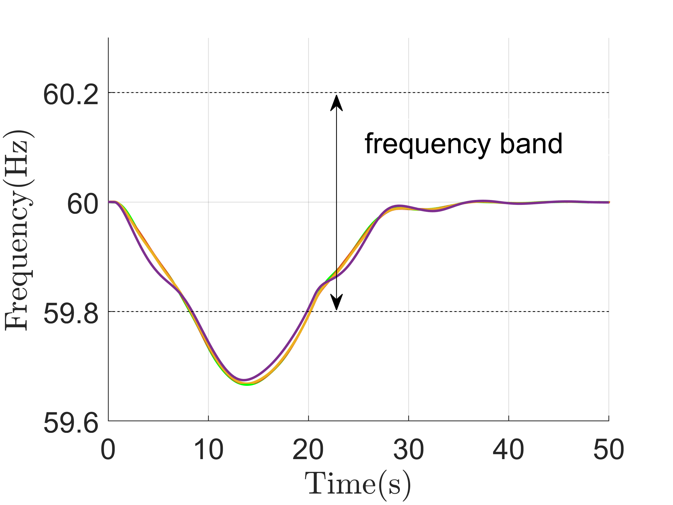
(a)

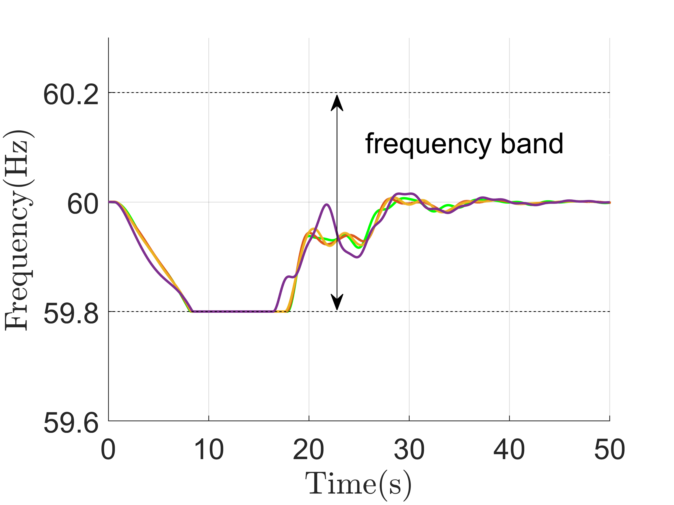
(b)

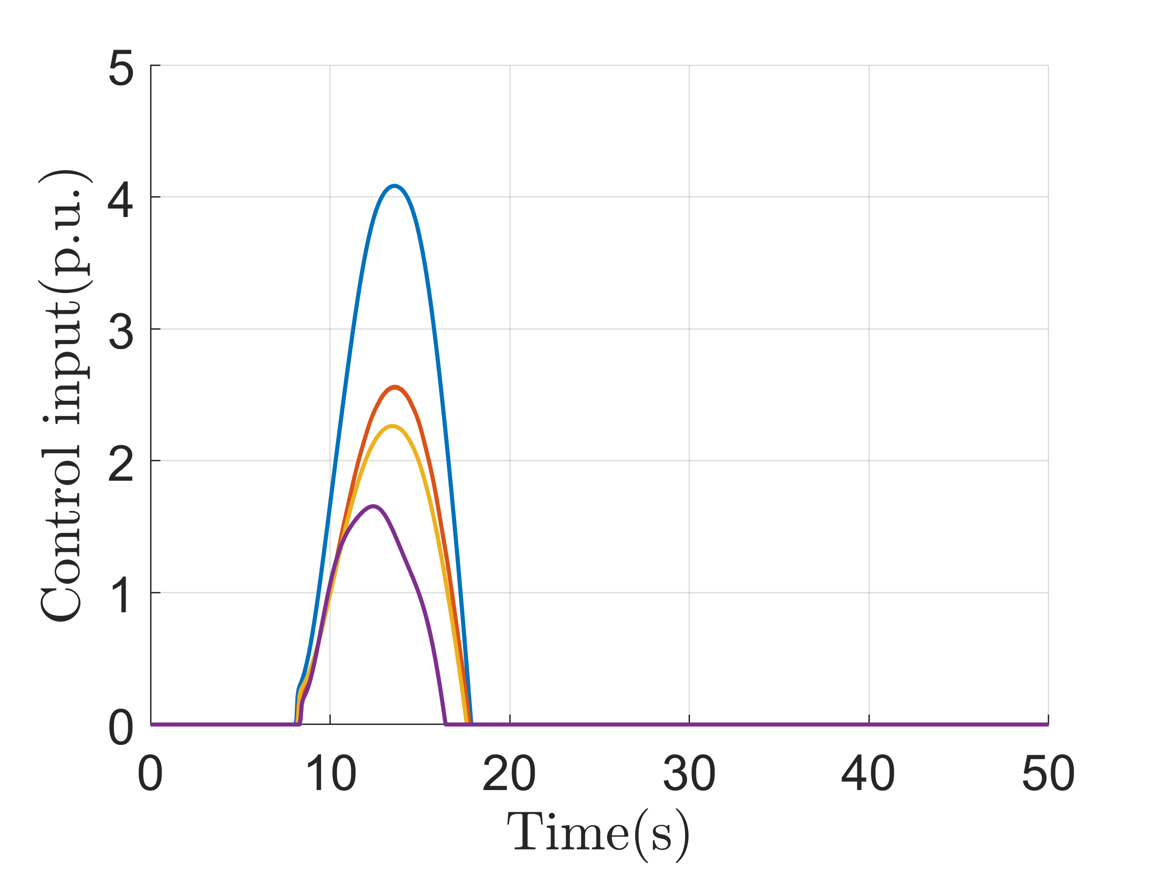
(c)

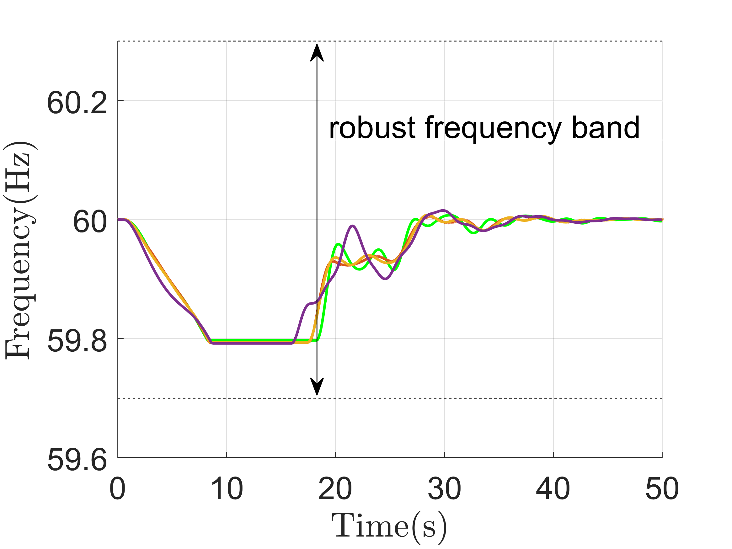
(d)

Figure 2: Frequency and control input trajectories with and without transient controller.

We first show that the proposed controller is able to maintain the targeted generator frequencies within the safe region, provided that these frequencies are initially in the safe region. We perturb all non-generator nodes by a sinusoidal power injection whose magnitude is proportional to the corresponding node’s initial power injection. Specifically, for every $i\in\{1,2,\cdots,29\}$,

$$p_{i}(t)=\begin{cases}p_{i}(0)&\text{if $t\leqslant 0.5$ or $t\geqslant 20.5$,}\\ \left(1+0.3\sin(\frac{\pi}{20}(t-0.5))\right)p_{i}(0)&\text{otherwise.}\end{cases}$$

For $i\in\{30,31,\cdots,39\}$, $p_{i}(t)$ remains constant all the time. Figure 22(a) shows the frequency responses of the 4 generators without the transient controller. One can easily see that all trajectories exceed the 59.8Hz lower frequency bound. For comparison, Figure 22(b) shows the trajectories with the transient controller (10), where one can see that all remain within the safe frequency region. Figure 22(c) displays the corresponding input trajectories, which converge to 0 in finite time, as stated in Theorem V.3(iii). The control input with highest overshoot corresponds to the generator $33$. Its large magnitude, compared to the other inputs, is due to the power flow in the adjacent edge $(19,33)$ evolving relatively far from the nominal value, resulting in a large power injection fluctuation to node $33$, which further causes a large control effort for compensation. We also illustrate the robustness of the controller against uncertainty. We have each controller employ $\hat{E}_{i}=2$ and $\hat{p}_{i}(t)=1.1p_{i}(t)$, corresponding to $100\%$ and $10\%$ deviations on droop coefficients and power injections, respectively. Figure 22(d) illustrates the frequency trajectories of the 4 controlled generators. Since condition (11) is satisfied with $\Delta=0.1$Hz, Proposition V.6 ensures that the frequency interval with invariance guarantee is now $[59.7\text{Hz},60.3\text{Hz}]$ (in fact, the four trajectories only slightly exceed $59.8$Hz).

Next, we examine the effect of the choice of class-$\mathcal{K}$ function on the behavior of the transient frequency. We focus our attention on bus $30$ and simulate the network behavior for two extreme values, $0.01$ and $100$, of the tunable parameter $\gamma_{30}$. Figure 3 shows the corresponding frequency and control input trajectories for the first 20 seconds at node 30. From Figure 33(a), one can see that the frequency trajectory with $\gamma_{30}=0.01$ tends to stay away from the lower safe bound (overprotection), compared with the trajectory with large $\gamma_{30}=100$, which results in a larger control input, as shown in Figure 33(b). Also, the control input with $\gamma_{30}=0.01$ is triggered earlier around $6$s. However, choosing a large $\gamma_{30}$ may lead to high sensitivity. We observe this in Figure 33(b), as the input trajectory with $\gamma_{30}=100$ grows faster around $8$s, compared to that with $\gamma_{30}=0.01$ does. These simulations verify our observations in Remark V.4.

(a)

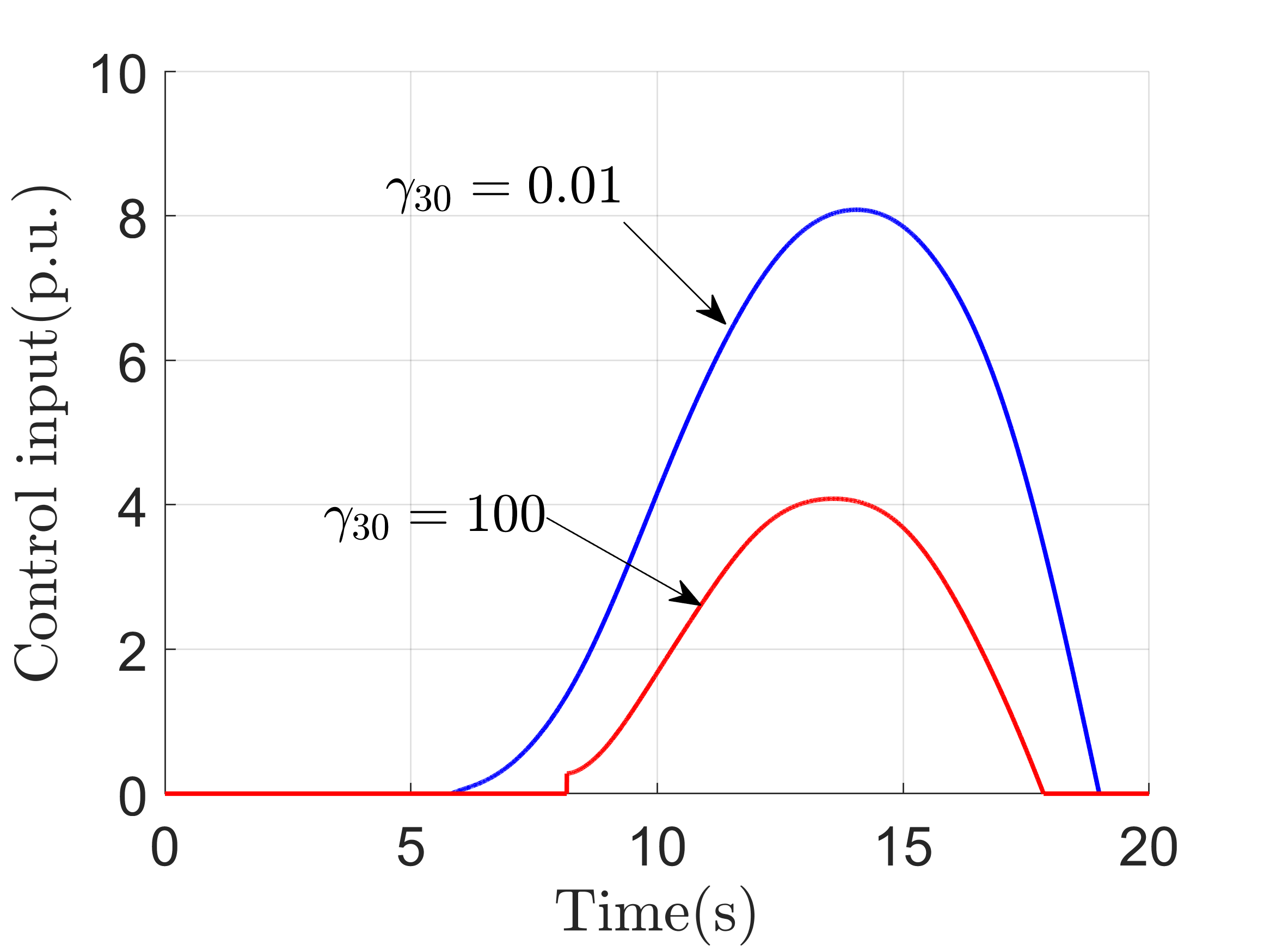
(b)

Figure 3: Frequency and control input trajectories at node $30$ with linear class-$\mathcal{K}$ function with slope $\gamma_{30}=0.01$ and $10$, respectively.

Lastly, we simulate the case where some of the generator frequencies are initially outside the safe frequency region to show how the transient controller brings the frequencies back to the safe region. To do so, we use the same setup as in Figure 2, but we only turn on the distributed controller after $t=10s$. Figure 44(a) shows the frequency trajectories of the 4 generators. As the controller is disabled for the first $10$s, all 4 frequency trajectories are lower than 59.8Hz at $t=10$s. After $t=10$s, all of them return to the safe region in a monotonic way, and once they are in the region, they never leave, in accordance with Theorem V.3(v). Figure 44(b) shows the corresponding control input trajectories.

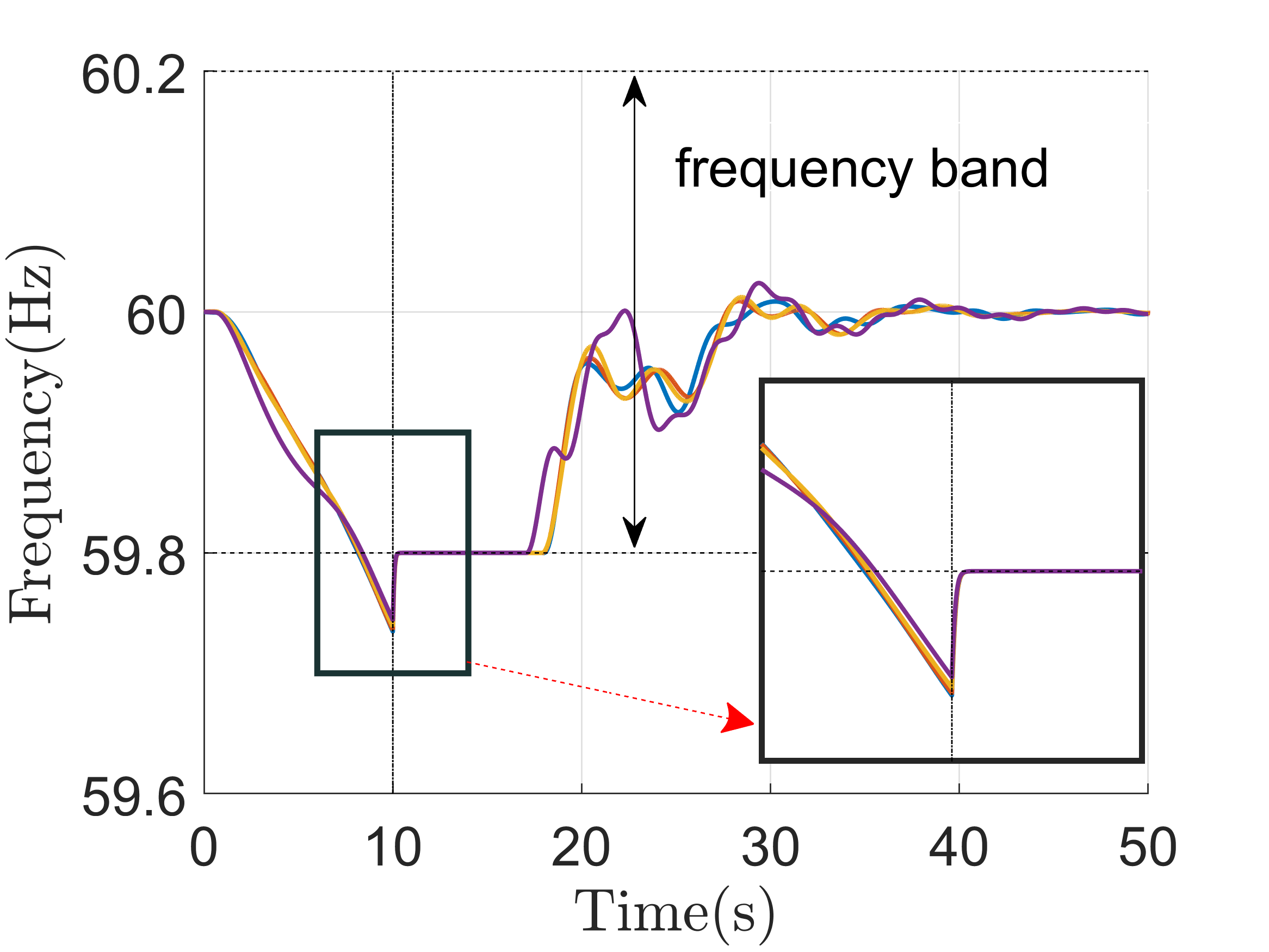
(a)

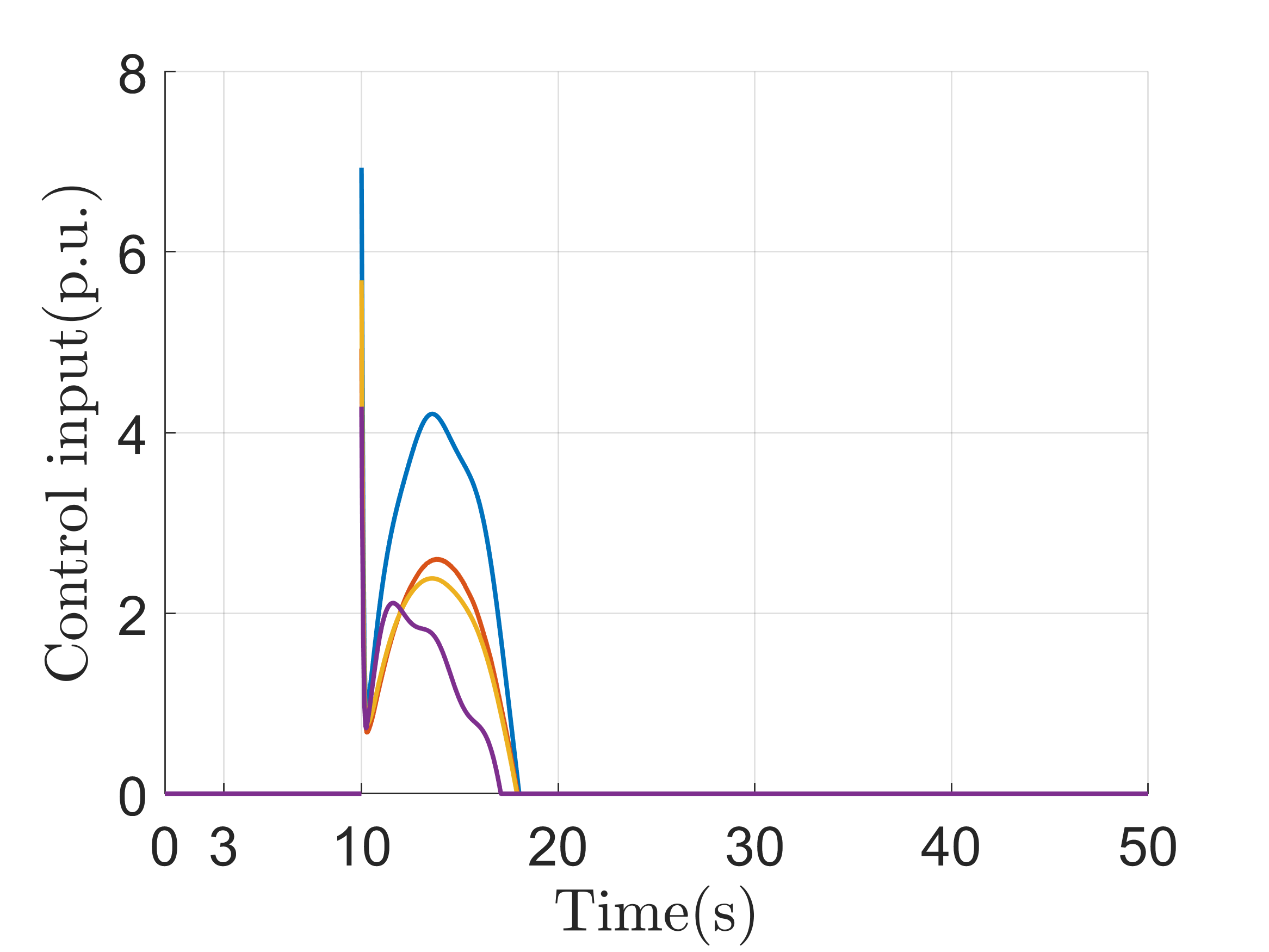
(b)

Figure 4: Frequency and control input trajectories with transient controller available after $t=10$s.

VII Conclusions

We have proposed a distributed transient frequency controller on a power network that is able to maintain the nodal frequency of the actuated buses within a given safe frequency region, and to recover it from undesired initial conditions. We have proven that the control input vanishes in finite time, so that the closed-loop system possesses the same equilibrium and asymptotic convergence guarantees as the open-loop one. Future work will investigate the extension to nonlinear power flow models with mechanical dynamics on generators, the incorporation of economic cost and actuator constraints in the controller design, the amelioration of control effort by having controlled nodes have access to information beyond their neighbors, and understanding of the connection between actuation effort and network connectivity.

References

- [1] P. Kundur, J. Paserba, V. Ajjarapu, G. Andersson, A. Bose, C. Canizares, N. Hatziargyriou, D. Hill, A. Stankovic, C. Taylor, T. V. Cutsem, and V. Vittal, “Definition and classification of power system stability,” IEEE Transactions on Power Systems, vol. 19, no. 2, pp. 1387–1401, 2004.
- [2] H. D. Chiang, Direct Methods for Stability Analysis of Electric Power Systems: Theoretical Foundation, BCU Methodologies, and Applications. John Wiley and Sons, 2011.
- [3] F. Dörfler, M. Chertkov, and F. Bullo, “Synchronization in complex oscillator networks and smart grids,” Proceedings of the National Academy of Sciences, vol. 110, no. 6, pp. 2005–2010, 2013.
- [4] P. J. Menck, J. Heitzig, J. Kurths, and H. J. Schellnhuber, “How dead ends undermine power grid stability,” Nature Communications, vol. 5, no. 3969, pp. 1–8, 2014.
- [5] P. Kundur, Power System Stability and Control. McGraw-Hill, 1994.
- [6] A. Alam and E. Makram, “Transient stability constrained optimal power flow,” in IEEE Power and Energy Society General Meeting, Montreal, Canada, Jun. 2006, electronic proceedings.
- [7] T. T. Nguyen, V. L. Nguyen, and A. Karimishad, “Transient stability-constrained optimal power flow for online dispatch and nodal price evaluation in power systems with flexible ac transmission system devices,” IET Generation, Transmission & Distribution, vol. 5, pp. 332–346, 2011.
- [8] M. A. Mahmud, H. R. Pota, M. Aldeen, and M. J. Hossain, “Partial feedback linearizing excitation controller for multimachine power systems to improve transient stability,” IEEE Transactions on Power Systems, vol. 29, pp. 561–571, 2014.
- [9] T. S. Borsche, T. Liu, and D. J. Hill, “Effects of rotational inertia on power system damping and frequency transients,” in IEEE Conf. on Decision and Control, Osaka, Japan, 2015, pp. 5940–5946.
- [10] B. K. Poolla, S. Bolognani, and F. Dorfler, “Optimal placement of virtual inertia in power grids,” IEEE Transactions on Automatic Control, 2017, to appear.
- [11] M. Althoff, “Formal and compositional analysis of power systems using reachable sets,” IEEE Transactions on Power Systems, vol. 29, no. 5, pp. 2270–2280, 2014.
- [12] Y. C. Chen and A. D. Domínguez-García, “A method to study the effect of renewable resource variability on power system dynamics,” IEEE Transactions on Power Systems, vol. 27, no. 4, pp. 1978–1989, 2012.
- [13] Y. Zhang and J. Cortés, “Transient-state feasibility set approximation of power networks against disturbances of unknown amplitude,” in American Control Conference, Seattle, WA, May 2017, pp. 2767–2772.
- [14] A. D. Ames, X. Xu, J. W. Grizzle, and P. Tabuada, “Control barrier function based quadratic programs for safety critical systems,” IEEE Transactions on Automatic Control, vol. 62, no. 8, pp. 3861–3876, 2017.
- [15] F. Blancini and S. Miani, Set-theoretic Methods in Control. Boston, MA: Birkhäuser, 2008.
- [16] F. Bullo, J. Cortés, and S. Martínez, Distributed Control of Robotic Networks, ser. Applied Mathematics Series. Princeton University Press, 2009, electronically available at http://coordinationbook.info.
- [17] N. Biggs, Algebraic Graph Theory, 2nd ed. Cambridge University Press, 1994.
- [18] C. Zhao, U. Topcu, N. Li, and S. H. Low, “Design and stability of load-side primary frequency control in power systems,” IEEE Transactions on Automatic Control, vol. 59, no. 5, pp. 1177–1189, 2014.
- [19] E. Mallada, “Distributed network synchronization: The internet and electric power grids,” Ph.D. dissertation, Cornell University, 2014, electronically available at http://www.its.caltech.edu/~mallada/pubs/2014/thesis.pdf.
- [20] J. Machowski, J. W. Bialek, and J. R. Bumby, Power System Dynamics: Stability and Control. Chichester, England: Wiley, 2008.
- [21] K. W. Cheung, J. Chow, and G. Rogers, Power System Toolbox, v 3.0. Rensselaer Polytechnic Institute and Cherry Tree Scientific Software, 2009.