One-point and two-point statistics of
homogeneous isotropic decaying turbulence
with variable viscosity

Abstract

The decay of homogeneous isotropic turbulence in a variable viscosity fluid with a viscosity ratio up to 15 is analyzed by means of highly resolved direct numerical simulations (DNS) at low Reynolds numbers. The question addressed by the present work is how quantities such as the kinetic energy and the associated dissipation rate, as well as the inter-scale transport mechanism of turbulence are changed by local fluctuations of the viscosity. From the one-point budget equation of the turbulent kinetic energy, it is shown that the mean dissipation rate is nearly unchanged by variable viscosity effects. This result is explained by a negative correlation between the local viscosity and the local velocity gradients. However, the dissipation is a highly fluctuating quantity with a strong level of intermittency. From a statistical analysis it is shown that turbulent flows with variable viscosity are characterized by an enhanced level of small-scale intermittency, which results in the presence of smaller length scales and a modified turbulent mixing. The effect of variable viscosity on the turbulent cascade is analyzed by a budget equation for the velocity structure function. From DNS it is shown that viscosity gradients contribute to the inter-scale transport mechanism in the form of an inverse transport, where information propagates from the small scales to the large scales.

1 Introduction

Turbulent flows encountered in engineering and environmental applications are very often characterized by spatio-temporal fluctuations of viscosity, which results from variations of temperature or species composition. A prominent example from geophysical flows is the convection in the earth’s mantle, where the viscosity decreases with temperature. An other important case is the turbulent mixing in combustion systems, where a concentration dependent viscosity may affect the efficiency of turbulent mixing.

Fully developed turbulence reveals a large range of length scales, varying from the so-called integral length scale $l_{t}$, at which large velocity fluctuations occur on average, down to the smallest scale, the so-called Kolmogorov or dissipation scale $\eta$, at which turbulent fluctuations are dissipated due to viscosity. According to Kolmogorov’s first hypothesis (Kolmogorov (1941a, b)), the statistics of the smallest scales should be universal, and depend only on two parameters, namely the viscosity $\nu$ and the mean energy dissipation rate $\langle{\varepsilon}\rangle$. Kolmogorov’s second hypothesis postulates that large scales of the flow decouple from the smallest scales and should become independent of viscosity, provided that the Reynolds number is sufficiently high. However, numerous experimental and numerical studies have indicated that Kolmogorov’s traditional view is a crude assumption and that large and small scale quantities are strongly coupled, cf. Sreenivasan and Antonia (1997), Warhaft (2000), and Antonia et al. (2015). The situation is even more complex for turbulent mixing with local viscosity variations. One has to cope with a turbulence-scalar interaction which is two-fold: the fluid motions affect the scalar mixing, while mixing induced viscosity changes affect the dynamics of the velocity field.

Viscosity represents the most important property of turbulent flows, and the impact of its variation on the dynamics should be addressed in detail. Most studies reported in literature have focused on the impact of variable viscosity on the large scales. Chhabra et al. (2005) and Talbot et al. (2013) studied turbulent jet flows, where the viscosity between jet fluid and host fluid differs. They observed, compared to a flow with uniform viscosity, that the relationship between production and dissipation of turbulent energy is altered and that the entrainment and the spreading rates of the jet flow are changed. An altered spreading rate was also observed by direct numerical simulations of turbulent shear layers with variable viscosity by Taguelmimt et al. (2016a, b) indicating the ability of viscosity variations to modify the largest scales of the flow. Voivenel et al. (2017) derived generalized scale-by-scale budget equations for velocity increments in inhomogeneous and anisotropic turbulence with variable viscosity. Based on this work, Danaila et al. (2017) showed that variable viscosity effects can invalidate the self-similarity of turbulent jet flows. The analysis of Lee et al. (2008) focused on the turbulent mixing of two initially segregated fluids with different viscosity in homogeneous isotropic turbulence. They found that the dissipation becomes independent of viscosity confirming Taylor’s postulate. Taylor (1935) postulated that the mean energy dissipation $\langle{\varepsilon}\rangle$ depends only on the large-scale velocity fluctuations $u^{\prime}$ and the integral length scale $l_{t}$, i.e.

$$\langle{\varepsilon}\rangle\propto\frac{u^{\prime 3}}{l_{t}}\,,$$ (1)

and hence becomes independent of viscosity, provided that the Reynolds number is sufficiently large. In eq. (1), the characteristic large-scale velocity fluctuations are defined as

$$u^{\prime}=\sqrt{\langle{u_{i}^{2}}\rangle/3}\,,$$ (2)

and the integral length scale $l_{t}$ is defined as

$$l_{t}=\frac{3\pi}{4}\frac{\int\kappa^{-1}E(\kappa,t){\rm d}\kappa}{\int E(\kappa,t){\rm d}\kappa}\,,$$ (3)

with $E(\kappa)$ being the three-dimensional energy spectrum and $\kappa$ the magnitude of the wave-number vector. Ensemble-averages are denoted by angular brackets and Einstein’s summation convention is used, which implies summation over indices appearing twice.

In this paper, we investigate the decay of homogeneous isotropic turbulence in a variable viscosity fluid by means of highly resolved direct numerical simulations (DNS). We address the question how quantities such as the kinetic energy and the associated dissipation rate, as well as the inter-scale transport mechanism of turbulence are changed by local fluctuations of the viscosity. The paper is structured as follows. Section 2 presents the governing equations and the direct numerical simulations on which the analysis is based. Section 3 introduces the budget equation of the turbulent energy and discusses the impact of variable viscosity on the dissipation mechanism of turbulence. Section 4 addresses the impact of variable viscosity on the viscous cut-off scales of turbulence. An analysis of the inter-scale transport mechanism based on a budget equation for the second-order velocity structure function is presented in section 5. We summarize this study in section 6.

2 Direct numerical simulations and governing equations

Direct numerical simulations of homogeneous isotropic turbulence with variable viscosity at three different viscosity ratios between 1 and 15 have been performed. The DNS solves the three-dimensional incompressible Navier-Stokes equations,

$$\frac{\partial u_{j}}{\partial t}+u_{i}\frac{\partial u_{j}}{\partial x_{i}}=-\frac{\partial p}{\partial x_{j}}+\frac{\partial}{\partial x_{i}}\left(2\nu s_{ij}\right)\,,$$ (4)

with the continuity equation

$$\frac{\partial u_{i}}{\partial x_{i}}=0\,,$$ (5)

in a triply periodic box with size $2\pi$ by a pseudo-spectral method. In eqs. (4) and (5), the velocity field is denoted by $u_{j}$, $p$ is the pressure (for simplicity the density $1/\rho$ is incorporated in $p$), $\nu$ is the local viscosity, and $s_{ij}$ is the strain-rate tensor, defined as

$$s_{ij}=\frac{1}{2}\left(\frac{\partial u_{j}}{\partial x_{i}}+\frac{\partial u_{i}}{\partial x_{j}}\right)\,.$$ (6)

The local viscosity field $\nu(\boldsymbol{x},t)$ is determined by solving an advection-diffusion equation for a scalar field $\phi(\boldsymbol{x},t)$, i.e.

$$\frac{\partial\phi}{\partial t}+u_{i}\frac{\partial\phi}{\partial x_{i}}=D\frac{\partial^{2}\phi}{\partial x_{i}^{2}}\,.$$ (7)

The scalar $\phi$ is statistically isotropic and homogeneous. For numerical convenience the scalar is further bounded, i.e. $-1\leq\phi(\boldsymbol{x},t)\leq 1$, and has zero mean, i.e. $\langle{\phi}\rangle=0$. Ensemble-averages are computed due to homogeneity over the full computational domain. The local viscosity $\nu(\boldsymbol{x},t)$ is linked through a linear relation to the scalar field, e.g. Gréa et al. (2014)

$$\nu(\boldsymbol{x},t)=\langle{\nu}\rangle+\nu^{\prime}(\boldsymbol{x},t)=\langle{\nu}\rangle+c\phi(\boldsymbol{x},t)\,,$$ (8)

where $\langle{\nu}\rangle$ denotes the uniform mean viscosity, $\nu^{\prime}(\boldsymbol{x},t)$ denotes the fluctuating viscosity field, and $c$ is a positive constant with $c<\langle{\nu}\rangle$ to ensure positivity of $\nu(\boldsymbol{x},t)$. A linear relation between $\nu$ and $\phi$ is convenient because it keeps the mean viscosity $\langle{\nu}\rangle$ unchanged during the decay. The constant $c$ is obtained from the initial minimum and maximum values of the viscosity by $c=(\nu_{\rm max}-\nu_{\rm min})/2$, which implies that the initial scalar variance $\langle{\phi^{2}}\rangle$ equals unity. In the following, we use $\phi$ as a surrogate for $\nu$. The molecular diffusivity $D$ in eq. (7) is assumed to be constant and equals the mean viscosity $\langle{\nu}\rangle=(\nu_{\rm min}+\nu_{\rm max})/2$. As a consequence, the Schmidt number, defined as $\mathit{Sc}=\nu/D$, is a fluctuating quantity.

The following paragraph briefly summarizes the main features of the DNS. More details about the numerical procedure and the parallelization approach are given by Gauding et al. (2015, 2017). Adapting the approach by Mansour and Wray (1994), the Navier-Stokes equations are formulated in spectral space as

$$\frac{\partial}{\partial t}\left(\hat{u}_{i}\exp(\nu\kappa^{2}t)\right)=\exp(\nu\kappa^{2}t)P_{ij}\hat{H}_{j}\,,$$ (9)

where

$$\hat{H}_{j}=-i\kappa_{i}\mathcal{F}\left(u_{i}u_{j}-2c\phi(\boldsymbol{x},t)s_{ij}\right)$$ (10)

is the Fourier transform of the non-linear terms, including the convective term and the non-linear part of the viscous term. The wave-number vector is denoted by $\boldsymbol{\kappa}$, and the Fourier transform of the velocity field is denoted by $\hat{\boldsymbol{u}}$. The projection operator $P_{ij}=\delta_{ij}-\kappa_{i}\kappa_{j}/\kappa^{2}$ imposes incompressibility. The non-linear terms are computed in physical space and a truncation technique with a smooth spectral filter is applied to remove aliasing errors. The smooth spectral filter is highly localized in both real and spectral space, and was found to be dynamically very stable, cf. Hou and Li (2007). This feature is relevant for the present study to prevent instabilities at high wave-number modes caused by the non-linear part of the viscous term. An integrating factor technique is used for an exact integration of the linear part of the viscous terms. Temporal integration is performed by a low-storage, stability preserving, third-order Runge-Kutta scheme. An additional necessary constraint that has to be satisfied by the DNS is an adequate resolution of the smallest scales. As proposed by Mansour and Wray (1994), we require that for all times, the condition $\kappa_{\rm max}\eta_{0}\geq 1$ is satisfied, where $\eta_{0}=(\langle{\nu}\rangle^{3}/\langle{\varepsilon}\rangle)^{1/4}$ is the Kolmogorov length scale and $\kappa_{\rm max}$ is the largest resolved wave-number. A grid resolution of $1024^{3}$ points is used to appropriately account for both small and large scales.

Let us now turn our attention to the initialization of the DNS. For the velocity field, we follow the approach of Ishida et al. (2006) and prescribe a broad-band energy spectrum of the type

$$E(\kappa,t=0)\propto\kappa^{4}\exp(-2(\kappa/\kappa_{p})^{2})\,.$$ (11)

The peak of the initial spectrum is located at $\kappa_{p}=12$ to inject energy at sufficiently large length scale while keeping the initial integral length scale $l_{t}$ small compared to the confinement imposed by the computational domain. The initialization guarantees that turbulence is statistically homogeneous, isotropic, and incompressible. The initial Reynolds number, defined with the mean viscosity as $\mathit{Re}_{0}=u^{\prime}/(\kappa_{p}\langle{\nu}\rangle)$, equals 43.

In this work, we compare three different DNS. The baseline case has a constant and spatially uniform viscosity of $\langle{\nu}\rangle=0.006$. Additionally, two cases with variable viscosity are considered. These cases have the same mean viscosity $\langle{\nu}\rangle$ as the baseline case, but an initial viscosity ratio $R_{\nu}=\nu_{\rm max}/\nu_{\rm min}$ that equals 5 and 15, respectively. The initial viscosity distribution is bi-modal with an initial normalized viscosity variance of $\langle{\nu^{\prime 2}}\rangle/\langle{\nu}\rangle^{2}=(\nu_{\rm max}-\nu_{\rm min})^{2}/(\nu_{\rm max}+\nu_{\rm min})^{2}$. At later times, the viscosity distribution is smoothed due to turbulent mixing, so that the viscosity variance $\langle{\nu^{\prime 2}}\rangle$ decreases. The initial scalar energy spectrum is proportional to the velocity spectrum, but the initial scalar field is not correlated with the velocity field, i.e. $\langle{u_{i}\phi}\rangle=0$. As the mean viscosity $\langle{\nu}\rangle$ stays constant during the decay, the differences between the cases can be attributed solely to the viscosity ratio $R_{\nu}$.

3 Budget of the one-point turbulent kinetic energy

An important question addressed by the present work is how the dissipation mechanism of turbulence is changed by variable viscosity, and whether turbulent flows with variable viscosity dissipate more or less energy as flows with constant viscosity. To answer this question, we first examine the transport equation for the mean turbulent kinetic energy $\langle{k}\rangle=\langle{u_{i}u_{i}}\rangle/2$, which reads in decaying homogeneous isotropic turbulence

$$\frac{\mbox{d}\langle{k}\rangle}{\mbox{d}t}=\left\langle\frac{\partial\nu}{\partial x_{i}}\frac{\partial}{\partial x_{j}}\left(u_{i}u_{j}\right)\right\rangle-\langle{\varepsilon}\rangle_{\rm VV}\,.$$ (12)

The first term on the right-hand side describes the dissipation of turbulent energy due to viscosity gradients. This term is negligible compared to the second term, which is the mean dissipation rate

$$\left\langle\varepsilon\right\rangle_{\rm VV}=\left\langle\nu\left(\frac{\partial u_{i}}{\partial x_{j}}\right)^{2}\right\rangle$$ (13)

of the turbulent kinetic energy $\langle{k}\rangle$. Figure 1 shows the temporal evolution of the mean turbulent kinetic energy $\langle{k}\rangle$. The mean turbulent kinetic energy is virtually unaffected by variable viscosity effects, and only a slightly reduced initial decay is visible for the cases with $R_{\nu}>1$. These results confirm the trends previously reported by Taguelmimt et al. (2016a, b) in DNS studies of temporally evolving mixing layers.

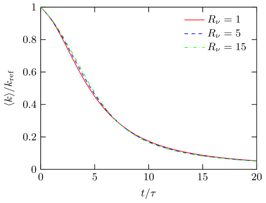
Figure 1: Temporal evolution of the mean turbulent kinetic energy $\langle{k}\rangle$ for the three viscosity ratios $R_{\nu}$. The time is normalized by $\tau=1/(\kappa_{p}u^{\prime}_{0})$, and $k_{\rm ref}=\langle{k}\rangle(t=0)$.

The mean dissipation $\langle{\varepsilon}\rangle_{\rm VV}$ is defined as the correlation between the local viscosity $\nu$ and the square of the local velocity gradient tensor

$$A_{ij}=\frac{\partial u_{i}}{\partial x_{j}}\,.$$ (14)

$\langle{\varepsilon}\rangle_{\rm VV}$ can be further decomposed by virtue of eq. (8) as

$$\langle{\varepsilon}\rangle_{\rm VV}=\underbrace{\langle{\nu}\rangle\left\langle{\left(\frac{\partial u_{i}}{\partial u_{j}}\right)^{2}}\right\rangle}_{\varepsilon_{CV}}+\underbrace{\left\langle{\nu^{\prime}\left(\frac{\partial u_{i}}{\partial u_{j}}\right)^{2}}\right\rangle}_{\varepsilon_{\nu^{\prime}}}\,.$$ (15)

The first term $\varepsilon_{CV}$ on the right-hand side of (15) denotes the classical dissipation for flows with constant viscosity, while the second term $\varepsilon_{\nu^{\prime}}$ accounts for dissipation due to fluctuations of the viscosity. Figure 2 shows the temporal evolution of the terms in (15) for the three cases under consideration. The mean dissipation $\langle{\varepsilon}\rangle_{\rm VV}$ displays an initial transient growth before turning into a decaying state, and is only slightly affected by the viscosity ratio $R_{\nu}$. During the transient period the increase of $\langle{\varepsilon}\rangle_{\rm VV}$ is delayed for the two cases with variable viscosity. During the early phase of the decay, $\langle{\varepsilon}\rangle_{\rm VV}$ of the variable viscosity cases exceeds the constant viscosity case, indicating an enhanced turbulent mixing process. At later times, when turbulent mixing advances and the amplitude of viscosity fluctuations decreases, no difference between the different cases can be discerned.

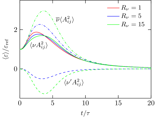
Figure 2: Temporal evolution of the terms in eq. (15), i.e. the mean dissipation rate $\langle{\varepsilon}\rangle_{\rm VV}=\langle{\nu A_{ij}^{2}}\rangle$ (solid lines), the dissipation formed with the mean viscosity $\langle{\varepsilon}\rangle_{\rm CV}=\langle{\nu}\rangle\langle{A_{ij}^{2}}\rangle$ (dashed-dotted lines) and the fluctuating part $\langle{\varepsilon}\rangle_{\nu^{\prime}}=\langle{\nu^{\prime}A_{ij}^{2}}\rangle$ (dashed lines). The latter term is not shown for $R_{\nu}=1$, as it is zero by definition. The time is normalized by $\tau=1/(\kappa_{p}u^{\prime}_{0})$. The reference dissipation is chosen as $\varepsilon_{\rm ref}=\langle{\varepsilon}\rangle(t=0)$.

Moreover, fig. 2 shows that different from $\langle{\varepsilon}\rangle_{\rm VV}$, both $\langle{\varepsilon}\rangle_{\rm CV}$ and $\langle{\varepsilon}\rangle_{\rm\nu^{\prime}}$ strongly depend on the viscosity ratio $R_{\nu}$. The dissipation $\langle{\varepsilon}\rangle_{\rm CV}$, which is built with the mean viscosity $\langle{\nu}\rangle$, is positive and increases with increasing viscosity ratio $R_{\nu}$ and clearly exceeds the mean dissipation $\langle{\varepsilon}\rangle_{\rm VV}$. As the mean viscosity $\langle{\nu}\rangle$ is the same for all cases, this indicates that turbulent flows with variable viscosity are characterized by larger velocity gradients $\langle{A_{ij}^{2}}\rangle$. In eq. (15), the strong dependence of $\langle{\varepsilon}\rangle_{\rm CV}$ on $R_{\nu}$ is compensated by the term $\langle{\varepsilon}\rangle_{\nu^{\prime}}$ formed with the fluctuating part of the viscosity $\nu^{\prime}$. Initially, $\langle{\varepsilon}\rangle_{\nu^{\prime}}$ is zero because viscosity fluctuations and velocity gradients are uncorrelated. During the transient period, $\langle{\varepsilon}\rangle_{\nu^{\prime}}$ becomes negative and tends to zero again for larger times. Due to the balance between the positive $\langle{\varepsilon}\rangle_{\rm CV}$ and the negative $\langle{\varepsilon}\rangle_{\nu^{\prime}}$, the mean dissipation $\langle{\varepsilon}\rangle_{\rm VV}$ is only slightly depending on $R_{\nu}$.

The conditional average $\langle{\varepsilon|\phi}\rangle$, shown in fig. 3, provides further information on the correlation between dissipation and viscosity. We discuss the temporal evolution of the normalized conditional dissipation $\langle{\varepsilon|\phi}\rangle$ to show how the dissipation adapts to viscosity as predicted by Taylor’s postulate, i.e.

$$\langle{\varepsilon|\phi}\rangle\propto\frac{u^{\prime 3}}{l_{t}}\,.$$ (16)

The general expectation is that the dissipation is independent of viscosity due to the fact that $l_{t}$ and $u^{\prime}$ are large scale quantities, which are virtually independent of fluctuations of the viscosity. However, Djenidi et al. (2017) showed within the framework of a scale-by-scale budget analysis that at finite Reynolds numbers, eq. (16) is strictly valid only in self-preserving turbulence. Figure 3 displays the conditional dissipation $\langle{\varepsilon|\phi}\rangle$ for three different time steps during the transition. A reference time is defined as $\tau=1/(\kappa_{p}u^{\prime}_{0})$. Shortly after initialization ($t/\tau=3.1$), the conditional dissipation $\langle{\varepsilon|\phi}\rangle$ is asymmetric for $R_{\nu}\neq 1$, signifying that the dissipation is not independent of viscosity. At this time, large dissipation values occur on average for $\phi>0$. At time step $t/\tau=6.2$, the dissipation decays but the decay rate is more rapid in the high-viscosity region (for $\phi>0$) and, hence, the asymmetry is inverted and the highest dissipation level is observed in the low viscosity regime for $\phi<0$. At later times ($t/\tau=9.3$), the conditional dissipation $\langle{\varepsilon|\phi}\rangle$ decays further but all curves virtually collapse and become independent of $\phi$. These findings justify the validity of Taylor’s postulate for turbulent flows with variable viscosity. The normalized dissipation becomes independent of viscosity after turbulence has adapted itself to the fluctuating viscosity field. A similar observation was made by Lee et al. (2008), by studying the turbulent mixing between two initially segregated fluids with vastly different viscosities. They found that during the mixing process, velocity gradients adapt rapidly to the viscosity field, and in less than one-half integral time, dissipation-viscosity independence was established.

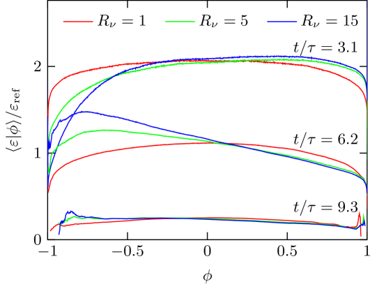
Figure 3: Mean dissipation $\langle{\varepsilon|\phi}\rangle$ conditioned on the scalar $\phi$ for three different times. The reference dissipation is defined as $\varepsilon_{\rm ref}=u^{\prime 3}_{0}\kappa_{p}$.

Let us now analyze the link between $\nu$ and $A_{ij}^{2}$ in more detail by probability density functions (pdf). To do this, we focus on the time step $t/\tau=9.3$, at which the dissipation has already adapted itself to the fluctuating viscosity field. This makes our analysis independent from transitional effects and reduces the impact of the initial conditions. An important feature of $A_{ij}^{2}$ (and the dissipation field) is the presence of large fluctuations, which exceed the respective mean values by orders of magnitude. This phenomenon is known in literature as internal intermittency, cf. Frisch (1995). Generally, the term intermittency describes a random process, which exhibits very strong events that occur more frequently than predicted by a Gaussian distribution. Following Nelkin (1994), the origin of intermittency lies in the non-linear dynamics of the vortex stretching mechanism. For variable viscosity turbulence, another source of intermittency can be identified by the non-linearity of the viscous term. To address this assertion, fig. 4 illustrates the normalized pdfs of $A_{ij}^{2}$ and $\varepsilon=\nu A_{ij}^{2}$ conditioned on $\phi\geq 0$ and $\phi<0$, respectively (note that $\nu$ is linearly related to $\phi$ by eq. (8)). The normalized pdf of $A_{ij}^{2}$ has stretched exponential tails, which originate from strong rare events that are non-universal and generally depend on Reynolds number. The far tails contribute mostly to higher-order moments and can be used to measure intermittency. From fig. 4, it can be observed that the tail of the $A_{ij}^{2}$ pdf in the low viscosity regime is significantly pronounced compared to the high viscosity regime. For comparison, the pdf of the constant viscosity case is shown. It has a less pronounced tail, compared to both low and high viscosity regimes of the variable viscosity case. This observation suggests that variable viscosity turbulence exhibits stronger fluctuations of the velocity gradients compared to constant viscosity turbulence at the same mean viscosity $\langle{\nu}\rangle$. This allows the conclusion that variable viscosity turbulence is characterized by an enhanced level of intermittency. A similar conclusion was drawn by Gréa et al. (2014) based on an EDQNM closure model. With this closure, they predicted that a variable viscosity fluid behaves like a fluid with constant but lower average viscosity, and therefore higher intermittency.

The normalized conditional pdf of the dissipation reveals a notably reduced dependence on viscosity, which signifies that statistics of the dissipation $\langle{{\varepsilon}}\rangle_{\rm VV}$ become independent of viscosity. This finding can be explained by the correlation $\nu$ and $A_{ij}^{2}$. Figure 5 shows that large velocity gradients occur on average at low viscosity (and vice versa). This negative correlation between $A_{ij}^{2}$ and $\nu^{\prime}$, i.e.

$$\langle{\nu^{\prime}A_{ij}^{2}}\rangle<0\,,$$ (17)

is a necessary condition for the independence of the dissipation from viscosity.

Figure 4: Normalized marginal pdf of $a=A_{ij}^{2}$ (top) and $\varepsilon=\nu A_{ij}^{2}$ (bottom), conditioned on positive and negative values of $\phi$. Note that $\nu$ is linearly related to $\phi$ by eq. (8). The curves are normalized by the individual mean values $\langle{\varepsilon}\rangle$ and $\langle{a}\rangle=\langle{A_{ij}^{2}}\rangle$, respectively. The figure shows the case $R_{\nu}=15$ at $t/\tau=9.3$. For reference, the constant viscosity case $R_{\nu}=1$ is shown.

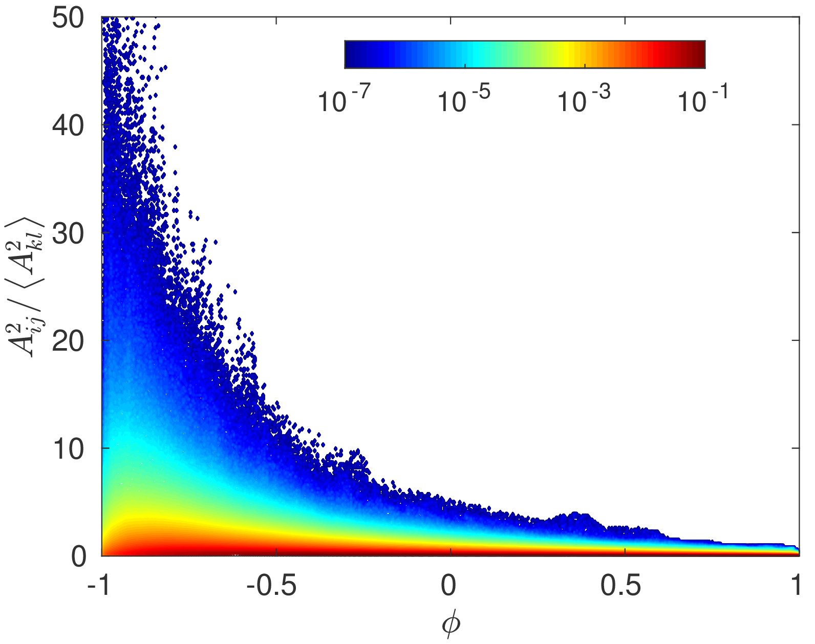
Figure 5: Joint pdf $P(A_{ij}^{2},\phi)$ indicates the presence of large velocity gradients especially in the low viscosity regime for $\phi<0$. The figure shows the case $R_{\nu}=15$ at $t/\tau=9.3$. The color is scaled logarithmically and increases in the sequence blue-green-yellow-red.

4 Impact of viscosity fluctuations on the viscous cut-off length scale

Kolmogorov’s scaling theory for turbulence (Kolmogorov (1941a, b)) postulates the existence of a dissipative cut-off scale where the turbulent cascade ends. This length scale is known as the Kolmogorov length scale

$$\eta_{0}=\left(\frac{\langle{\nu}\rangle^{3}}{\langle{\varepsilon}\rangle}\right)^{1/4}\,.$$ (18)

In a turbulent flow, high values of the local dissipation $\varepsilon$ occur around thin sheet or tube-like regions, which are characterized by length scales much smaller than the Kolmogorov length scale $\eta_{0}$ built with the mean viscosity $\langle{\nu}\rangle$ and mean dissipation $\langle{\varepsilon}\rangle$. To study fluctuations of the local dissipative cut-off scale, we follow Schumacher (2007) and introduce a local Kolmogorov length, defined as

$$\eta=\left(\frac{{\nu}^{3}}{{\varepsilon}}\right)^{1/4},$$ (19)

which is itself a fluctuating quantity. To quantify variations of the local Kolmogorov length $\eta$, the probability density function $P(\eta)$ is of interest. The normalized pdf of $\eta$ is displayed in fig. 6 for all cases, and shows that generally, length scales much smaller than $\eta_{0}$ exist. The left tail of the pdf, which is dominated by large intermittent fluctuations of the dissipation, reveals a strong dependence on the viscosity ratio $R_{\nu}$. The cases with variable viscosity show a clear tendency to establish significantly smaller cut-off scales than the case with constant viscosity. On the other hand, the right tail of the pdf is nearly unaffected by viscosity fluctuations. These findings indicate that particularly the strong intermittent events of turbulence are enhanced by the fluctuations of viscosity, resulting in the presence of smaller length scales and a modified turbulent mixing. A further justification of these results is provided by the joint pdf of the velocity gradients and the viscosity $P(A_{ij}^{2},\phi)$, where the largest velocity gradients $A_{ij}^{2}$ occur in the regime of low viscosity, see fig. 5. This observation signifies that the smallest length scales occur as expected in regions of low viscosity.

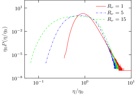
Figure 6: Normalized probability density function of the Kolmogorov length scale $\eta=(\nu^{3}/\varepsilon)^{1/4}$ at $t/\tau=9.3$.

To illustrate the impact of viscosity fluctuations on the local structure of turbulence, we display in fig. 7 iso-surfaces of the vorticity, defined by the Q-criterion

$$Q=\frac{1}{2}\left(\omega_{ij}^{2}-s_{ij}^{2}\right),$$ (20)

where $\omega_{ij}$ and $s_{ij}$ are the anti-symmetric and symmetric components of the velocity gradient tensor, respectively, cf. Dubief and Delcayre (2000). The iso-surfaces are colored by local viscosity. The turbulent field, defined by (20), is characterized by a high level of intermittency. Figure 7 reveals an enormous number of degrees of freedom represented by the interaction of vortices of different size that tend to cluster in coherent structures. A correlation between the local viscosity and the size of the vortex structures is clearly visible. Regions of low viscosity exhibit a fine vortex structure, while the size of vortex structures is considerably larger in regions of high viscosity. The reason for this observation is the damping effect of viscosity resulting in different local Reynolds numbers.

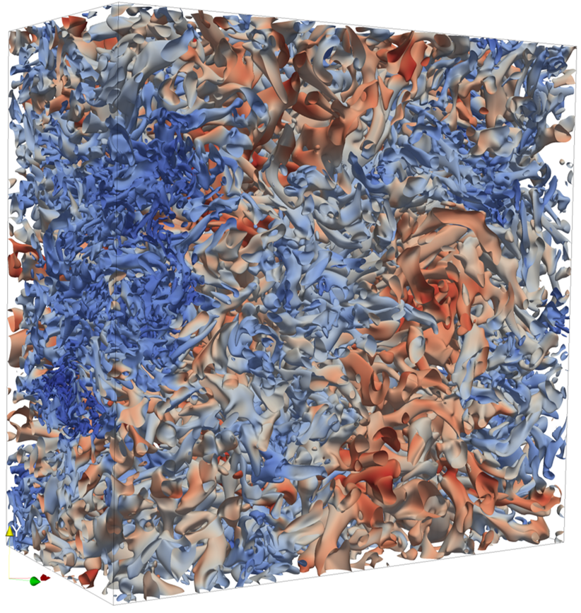
Figure 7: Iso-surface of vorticity defined by the Q-criterion, cf. Dubief and Delcayre (2000), for case $R_{\nu}=15$. The iso-surface is colored by local viscosity, where the color scale increases in the sequence blue-white-red.

5 Scale-by-scale budget equation for turbulence with variable viscosity

A central quantity of turbulence research is the velocity increment $\Delta u=u(\boldsymbol{x}+\boldsymbol{r})-u(\boldsymbol{x})$, defined as the velocity difference between two points separated by a distance $\boldsymbol{r}$. The moments of the velocity increment are known as structure functions. Transport equations for structure functions have been widely studied in literature and can be derived from first principles, cf. Danaila et al. (2001) and Gauding et al. (2014). Structure functions can be used to analyze scale-dependent properties, since they capture not only local but also non-local phenomena. We derived a novel transport equation for the so-called energy structure function $\langle{(\Delta u_{j})^{2}}\rangle$ for variable viscosity fluids. For statistically homogeneous incompressible turbulence, this equation reads

$$\frac{\partial}{\partial t}\langle{(\Delta u_{j})^{2}}\rangle+ \frac{\partial}{\partial r_{i}}\left\langle\Delta u_{i}(\Delta u_{j})^{2}\right\rangle=\frac{\partial^{2}}{\partial r_{i}^{2}}\langle{(\nu+\nu^{+})(\Delta u_{j})^{2}}\rangle\;$$ (21)

$$- 2\left\langle\nu\left(\frac{\partial u_{j}}{\partial x_{i}}\right)^{2}+{\nu^{+}\left(\frac{\partial u_{j}^{+}}{\partial x_{i}^{+}}\right)^{2}}\right\rangle$$

$$- \frac{\partial}{\partial r_{i}}\left\langle\left(\frac{\partial\nu^{+}}{\partial x_{i}^{+}}-\frac{\partial\nu}{\partial x_{i}}\right)(\Delta u_{j})^{2}\right\rangle\;$$

$$+ \left\langle\Delta u_{j}\left(\frac{\partial\nu^{+}}{\partial x_{i}^{+}}\frac{\partial u_{i}^{+}}{\partial x_{j}^{+}}-\frac{\partial\nu}{\partial x_{i}}\frac{\partial u_{i}}{\partial x_{j}}\right)\right\rangle\;.$$

The general procedure to derive eq. (21) is to formulate the Navier-Stokes equations at two different and independent points $\boldsymbol{x}$ and $\boldsymbol{x}^{+}$. For notational clarity, the super-script $+$ refers to quantities defined at the point $\boldsymbol{x}^{+}=\boldsymbol{x}+\boldsymbol{r}$. Subtracting the governing equations at these two points leads to an evolution equation for the velocity increment $\Delta u_{j}$. Multiplication of the result with $2\Delta u_{j}$ and ensemble-averaging gives eq. (21). Due to statistical homogeneity of the considered flow, the ensemble-averaged equation is independent of position $\boldsymbol{x}$, and depends solely on the separation vector $\boldsymbol{r}$.

Equation (21) is a generalized scale-by-scale budget equation for the turbulent energy at scale $r$ for turbulent flows with variable viscosity. The terms on the left-hand side represent unsteady effects and turbulent inter-scale transport. The first two terms on the right-hand side represent molecular inter-scale transport and dissipation of turbulent energy. The last two terms on the right-hand side occur only in turbulence with variable viscosity. They result from the viscous term of eq. (4) and represent inter-scale transport and molecular transport due to viscosity gradients. A scale-by-scale budget equation for variable viscosity turbulence was derived before by Voivenel et al. (2016) without discriminating between transport induced by turbulence and transport induced by viscosity gradients.

6 Analysis of scale-by-scale budget equations with constant and variable viscosity

In the following, we will analyze the DNS based on structure functions. First, we examine the longitudinal second-order velocity structure function $\langle{(\Delta u)^{2}}\rangle$ as it appears in the unsteady term. Then, the longitudinal mixed viscosity-velocity structure function $\langle{(\nu+\nu^{+})(\Delta u)^{2}}\rangle$ as it occurs in the diffusive term of eq. (21) will be discussed. After that, we turn our attention to the full budget as given by eq. (21) to analyze the impact of viscosity gradients on the inter-scale transport mechanism.

In the limit $r\to 0$, the second order structure function $\langle{(\Delta u)^{2}}\rangle$ can be developed in a Taylor series, i.e.

$$\langle{(\Delta u)^{2}}\rangle=\left\langle\left(\frac{\partial u}{\partial x}\right)^{2}\right\rangle r^{2}=\frac{1}{15}\frac{\langle{\varepsilon}\rangle_{\rm CV}}{\langle{\nu}\rangle}r^{2}\,,$$ (22)

and is uniquely determined by $\langle{\nu}\rangle$ and $\langle{\varepsilon}\rangle_{\rm CV}$. In the derivation of eq. (22) it is assumed without loss of generality that the separation vector $\boldsymbol{r}$ is aligned with the $x$ axis. In the second equality the factor $1/15$ is obtained by relating $\langle{\varepsilon}\rangle_{\rm CV}$ to $\langle{(\partial u/\partial x)^{2}}\rangle$ due to isotropy. In the large-scale limit for $r\to\infty$, the second order structure function becomes independent of $r$ and tends to its one-point limit, which equals $2\langle{u^{2}}\rangle$. Figure 8 shows the velocity structure function $\langle{(\Delta u)^{2}}\rangle$ for different times, for the constant and variable viscosity cases under consideration. The structure functions are compensated by the dissipative range scaling $r^{2}$, which yields a plateau for $r\to 0$. A dependence of the structure function on the viscosity ratio is observed in the dissipative range for the time steps $t/\tau=2.0$ and $t/\tau=3.1$, which is in agreement with the dependence of $\langle{A_{ij}^{2}}\rangle$ on $R_{\nu}$. At later times or at larger scales, $\langle{(\Delta u)^{2}}\rangle$ is independent of $R_{\nu}$, which is in agreement with the independence of $\langle{k}\rangle$ on $R_{\nu}$.

In a next step, we consider the viscosity-velocity structure function, defined as

$$S_{\nu}=\langle{(\nu(\boldsymbol{x}+\boldsymbol{r})+\nu(\boldsymbol{x}))(u(\boldsymbol{r}+\boldsymbol{r})-u(\boldsymbol{x}))^{2}}\rangle\,,$$ (23)

which appears in the diffusive term of the transport equation for $\langle{(\Delta u)^{2}}\rangle$ in variable viscosity turbulence, cf. eq. (21). Equation (23) can be developed in a Taylor-series for $r\to 0$, yielding

$$S_{\nu}=2\left\langle\nu\left(\frac{\partial u}{\partial x}\right)^{2}\right\rangle r^{2}\,.$$ (24)

In the large-scale limit $r\to\infty$, $S_{\nu}$ becomes independent of $r$ and tends to $4\langle{\nu u^{2}}\rangle$. Under the assumption that the viscosity is statistically independent from the turbulent energy, $4\langle{\nu u^{2}}\rangle$ simplifies to $4\langle{\nu}\rangle\langle{u^{2}}\rangle$. The viscosity-velocity structure functions are shown in fig. 8. Different to $\langle{(\Delta u)^{2}}\rangle$, the viscosity-velocity structure functions collapse for all time steps under consideration over all scales $r$ independently of $R_{\nu}$. This result underlines that large-scale statistics in statistical homogeneous isotropic turbulence are not affected by fluctuations of the viscosity due to the statistical independence between $u^{2}$ and $\nu$.

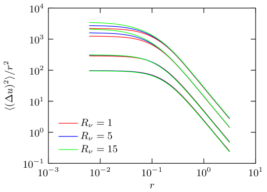
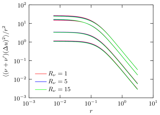
Figure 8: Compensated second order velocity structure function (top) and compensated mixed viscosity-velocity structure function (bottom) for different viscosity ratios $R_{\nu}$ and different times $t/\tau$ (the time steps $t/\tau=2.0$ (top-most), 3.1, 6.2, 9.3 (bottom-most) are displayed).

Provided that the Reynolds number is very large and with the assumptions of local isotropy and uniform viscosity, eq. (21) simplifies in inertial range for $\eta\gg r\gg l_{t}$ to

$$-\langle{\Delta u_{L}(\Delta u_{j})^{2}}\rangle=\frac{4}{3}\langle{\varepsilon}\rangle r\,,$$ (25)

where $\Delta u_{L}$ being the longitudinal velocity increment aligned with the separation vector $\boldsymbol{r}$, cf. Antonia et al. (1997). At low Reynolds numbers, a well established inertial range does not exist and we can generally not assume that inertial range statistics are independent of viscosity fluctuations. In this case, we need to consider all terms of eq. (21). The scale-by-scale budget, normalized by $4\langle{\varepsilon}\rangle_{\rm VV}$, is shown in fig. 9 for different $R_{\nu}$. It can be observed, that in the dissipative range the viscous terms $D(r)$, defined by

$$D(r)=\frac{\partial^{2}}{\partial r_{i}^{2}}\langle{(\nu+\nu^{+})(\Delta u_{j})^{2}}\rangle+\langle{\Delta u_{j}\left(\frac{\partial\nu^{+}}{\partial x_{i}^{+}}\frac{\partial u_{i}^{+}}{\partial x_{j}^{+}}-\frac{\partial\nu}{\partial x_{i}}\frac{\partial u_{i}}{\partial x_{j}}\right)}\rangle\,,$$ (26)

are relevant and balance in the limit $r\to 0$ the dissipation, i.e

$$\lim_{r\to 0}D(r)=4\langle{\varepsilon}\rangle_{\rm VV}\;.$$ (27)

At intermediate scales, $\eta\ll r\ll l_{t}$, two different inter-scale transport mechanisms exist, namely turbulent inter-scale transport

$$\mathit{Tr}_{t}=\frac{\partial}{\partial r_{i}}\langle{\Delta u_{i}(\Delta u_{j})^{2}}\rangle\,,$$ (28)

and inter-scale transport due to viscosity gradients

$$\mathit{Tr}_{\nu}=\frac{\partial}{\partial r_{i}}\langle{\left(\frac{\partial\nu^{+}}{\partial x_{i}^{+}}-\frac{\partial\nu}{\partial x_{i}}\right)(\Delta u_{j})^{2}}\rangle\,.$$ (29)

As shown in fig. 9, the inter-scale transport due to viscosity $\mathit{Tr}_{\nu}$ is small compared to the turbulent inter-scale transport $\mathit{Tr}_{t}$. Due to the relatively low Reynolds number, the flow does not exhibit a clear inertial range. The turbulent transport $\mathit{Tr}_{t}$ is negative, which confirms the well known forward cascade of turbulence with a mean transport of turbulent energy from the large scales towards the small scales. However, $\mathit{Tr}_{\nu}$ is positive implying that viscosity gradients induce an inverse transport, where energy propagates from the small scales to the large scales. This finding is important because it signifies that variable viscosity effects are not only limited to small scales, but can also affect larger scales as found by Voivenel et al. (2017) and Danaila et al. (2017) by studying the morphology of turbulent jet flows with variable viscosity. Similar observations have been made in the context of differential diffusion. Differential diffusion has a molecular origin and also reveals an inverse transport of energy from the small scales to the large scales, cf. Yeung (1996) and Hunger et al. (2016).

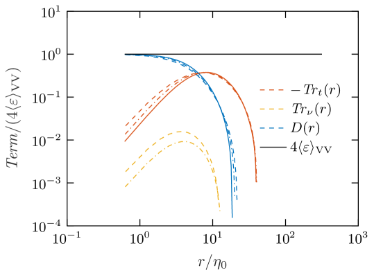
Figure 9: Scale-by-scale budget according to eq. (21) showing the viscous term $D(r)$, the turbulent inter-scale transport term $T_{t}(r)$, and the inter-scale transport term due to viscosity gradients $T_{\nu}(r)$ for different viscosity ratios $R_{\nu}=1$ (solid lines), $R_{\nu}=5$ (dashed lines), and $R_{\nu}=15$ (dashed-dotted lines). The scale-by-scale budget can be written with eqs. (26) - (29) as $\frac{\partial}{\partial t}\langle{(\Delta u_{j})^{2}}\rangle-\mathit{Tr}_{\nu}-\mathit{Tr}_{t}+D=4\langle{\varepsilon}\rangle_{\rm VV}$.

7 Summary and discussion

In the present study, we analyzed homogeneous isotropic decaying turbulence with variable viscosity at low Reynolds number by means of highly resolved direct numerical simulations. Three different viscosity ratios between 1 and 15 were considered.

The main results are:
(i) An analysis of the transport equation for the turbulent kinetic energy showed that the effect of variable viscosity is virtually negligible on both the mean turbulent energy $\langle{k}\rangle$ and the mean dissipation $\langle{\varepsilon}\rangle_{\rm VV}$. This finding is in agreement with previous observations by Lee et al. (2008) and Gréa et al. (2014). It confirms the validity of Taylor’s postulate, which states that the (normalized) dissipation is independent of viscosity.
(ii) Turbulent flows with variable viscosity reveal significantly enhanced velocity gradients in regions of low viscosity, which results in the presence of smaller length scales and an increased level of small-scale intermittency.
(iii) A generalized scale-by-scale budget equation for the energy structure function $\langle{(\Delta u_{j})^{2}}\rangle$ in variable viscosity flows was derived. A new term appears in this equation that accounts for an additional inter-scale transport due to viscosity gradients. This contribution is small compared to the turbulent inter-scale transport. But different to the turbulent inter-scale transport, the viscosity gradient induced transport is directed from the small scales to the large scales.

References

References

- Antonia et al. (1997) Antonia, R., Ould-Rouis, M., Anselmet, F., Zhu, Y., 1997. Analogy between predictions of Kolmogorov and Yaglom. Journal of Fluid Mechanics 332, 395–409.
- Antonia et al. (2015) Antonia, R., Tang, S., Djenidi, L., Danaila, L., 2015. Boundedness of the velocity derivative skewness in various turbulent flows. Journal of Fluid Mechanics 781, 727–744.
- Chhabra et al. (2005) Chhabra, S., Shipman, T. N., Prasad, A. K., 2005. The entrainment behavior of a turbulent axisymmetric jet in a viscous host fluid. Experiments in fluids 38 (1), 70–79.
- Danaila et al. (2001) Danaila, L., Anselmet, F., Zhou, T., Antonia, R., 2001. Turbulent energy scale budget equations in a fully developed channel flow. Journal of Fluid Mechanics 430, 87–109.
- Danaila et al. (2017) Danaila, L., Voivenel, L., Varea, E., 2017. Self-similarity criteria in anisotropic flows with viscosity stratification. Physics of Fluids 29 (2), 020716.
- Djenidi et al. (2017) Djenidi, L., Lefeuvre, N., Kamruzzaman, M., Antonia, R., 2017. On the normalized dissipation parameter in decaying turbulence. Journal of Fluid Mechanics 817, 61–79.
- Dubief and Delcayre (2000) Dubief, Y., Delcayre, F., 2000. On coherent-vortex identification in turbulence. Journal of Turbulence 1 (1), 011–011.
- Frisch (1995) Frisch, U., 1995. Turbulence: The legacy of AN Kolmogorov. Cambridge university press.
- Gauding et al. (2017) Gauding, M., Danaila, L., Varea, E., 2017. High-order structure functions for passive scalar fed by a mean gradient. International Journal of Heat and Fluid Flow.
- Gauding et al. (2015) Gauding, M., Goebbert, J. H., Hasse, C., Peters, N., 2015. Line segments in homogeneous scalar turbulence. Physics of Fluids 27 (9), 095102.
- Gauding et al. (2014) Gauding, M., Wick, A., Pitsch, H., Peters, N., 2014. Generalised scale-by-scale energy-budget equations and large-eddy simulations of anisotropic scalar turbulence at various Schmidt numbers. Journal of Turbulence 15 (12), 857–882.
- Gréa et al. (2014) Gréa, B.-J., Griffond, J., Burlot, A., 2014. The effects of variable viscosity on the decay of homogeneous isotropic turbulence. Physics of Fluids 26 (3), 035104.
- Hou and Li (2007) Hou, T. Y., Li, R., 2007. Computing nearly singular solutions using pseudo-spectral methods. Journal of Computational Physics 226 (1), 379–397.
- Hunger et al. (2016) Hunger, F., Gauding, M., Hasse, C., 2016. On the impact of the turbulent/non-turbulent interface on differential diffusion in a turbulent jet flow. Journal of Fluid Mechanics 802.
- Ishida et al. (2006) Ishida, T., Davidson, P., Kaneda, Y., 2006. On the decay of isotropic turbulence. Journal of Fluid Mechanics 564, 455–475.
- Kolmogorov (1941a) Kolmogorov, A. N., 1941a. Dissipation of energy in locally isotropic turbulence. In: Dokl. Akad. Nauk SSSR. Vol. 32. JSTOR, pp. 16–18.
- Kolmogorov (1941b) Kolmogorov, A. N., 1941b. The local structure of turbulence in incompressible viscous fluid for very large Reynolds numbers. In: Dokl. Akad. Nauk SSSR. Vol. 30. JSTOR, pp. 301–305.
- Lee et al. (2008) Lee, K., Girimaji, S. S., Kerimo, J., 2008. Validity of Taylor’s dissipation-viscosity independence postulate in variable-viscosity turbulent fluid mixtures. Physical review letters 101 (7), 074501.
- Mansour and Wray (1994) Mansour, N., Wray, A., 1994. Decay of isotropic turbulence at low Reynolds number. Physics of Fluids 6 (2), 808–814.
- Nelkin (1994) Nelkin, M., 1994. Universality and scaling in fully developed turbulence. Advances in physics 43 (2), 143–181.
- Schumacher (2007) Schumacher, J., 2007. Sub-kolmogorov-scale fluctuations in fluid turbulence. EPL (Europhysics Letters) 80 (5), 54001.
- Sreenivasan and Antonia (1997) Sreenivasan, K., Antonia, R., 1997. The phenomenology of small-scale turbulence. Annual review of fluid mechanics 29 (1), 435–472.
- Stephan and Docter (2015) Stephan, M., Docter, J., 2015. JUQUEEN: IBM Blue Gene/Q® supercomputer system at the Jülich supercomputing centre. Journal of large-scale research facilities JLSRF 1, 1.
- Taguelmimt et al. (2016a) Taguelmimt, N., Danaila, L., Hadjadj, A., 2016a. Effect of viscosity gradients on mean velocity profile in temporal mixing layer. Journal of Turbulence 17 (5), 491–517.
- Taguelmimt et al. (2016b) Taguelmimt, N., Danaila, L., Hadjadj, A., 2016b. Effects of viscosity variations in temporal mixing layer. Flow, Turbulence and Combustion 96 (1), 163–181.
- Talbot et al. (2013) Talbot, B., Danaila, L., Renou, B., 2013. Variable-viscosity mixing in the very near field of a round jet. Physica Scripta 2013 (T155), 014006.
- Taylor (1935) Taylor, G. I., 1935. Statistical theory of turbulence. In: Proceedings of the Royal Society of London A: Mathematical, Physical and Engineering Sciences. Vol. 151. The Royal Society, pp. 421–444.
- Voivenel et al. (2016) Voivenel, L., Danaila, L., Varea, E., Renou, B., Cazalens, M., 2016. On the similarity of variable viscosity flows. Physica Scripta 91 (8), 084007.
- Voivenel et al. (2017) Voivenel, L., Varea, E., Danaila, L., Renou, B., Cazalens, M., 2017. Variable viscosity jets: Entrainment and mixing process. In: Whither Turbulence and Big Data in the 21st Century? Springer, pp. 147–162.
- Warhaft (2000) Warhaft, Z., 2000. Passive scalars in turbulent flows. Annual Review of Fluid Mechanics 32 (1), 203–240.
- Yeung (1996) Yeung, P., 1996. Multi-scalar triadic interactions in differential diffusion with and without mean scalar gradients. Journal of Fluid Mechanics 321, 235–278.