Minimal Paths for Tubular Structure Segmentation with Coherence Penalty and Adaptive Anisotropy

Abstract

The minimal path method has proven to be particularly useful and efficient in tubular structure segmentation applications. In this paper, we propose a new minimal path model associated with a dynamic Riemannian metric embedded with an appearance feature coherence penalty and an adaptive anisotropy enhancement term. The features that characterize the appearance and anisotropy properties of a tubular structure are extracted through the associated orientation score. The proposed dynamic Riemannian metric is updated in the course of the geodesic distance computation carried out by the efficient single-pass fast marching method. Compared to state-of-the-art minimal path models, the proposed minimal path model is able to extract the desired tubular structures from a complicated vessel tree structure. In addition, we propose an efficient prior path-based method to search for vessel radius value at each centerline position of the target. Finally, we perform the numerical experiments on both synthetic and real images. The quantitive validation is carried out on retinal vessel images. The results indicate that the proposed model indeed achieves a promising performance.

I Introduction

Tubular structure segmentation plays an important role in many applications of image analysis and medical imaging [1, 2, 3]. A broad variety of significant approaches have been exploited to solve the tubularity segmentation problem in the passed decades. Among these models, the variational methods including the active contours models (e.g. [4, 5, 6]) and the minimal path models [7] have been successfully applied to various situations thanks to their solid theoretical background and the reliable numerical solvers.

The basic idea for the active contours approaches is to model the boundaries of a tubular structure through optimal curves or optimal surfaces, which are in general obtained by minimizing a functional relying on the image features extracted from the tubular structures. An interesting example is the flux-based active contours model [8] using the spherical flux of the image gradient vectors for tubular features computation. Lax and Chung [9] proposed an efficient way for the multi-scale spherical flux computation implemented by the fast Fourier transform in the Fourier domain. To improve the performance of the flux maximizing flow [8], the image gradient vector field can be replaced by more adequate problem-dependent vector fields [10, 11]. The authors of [12] proposed a new active contours functional involving the asymmetry measure of the image gradients and the symmetric oriented flux measure [13]. The constraints derived from the elongated nature of a tubular structure were taken into account in [14, 15, 16]. Cohen and Deschamps [17] combined the geodesic distance-based front propagation method [18] and a Euclidean curve length-based thresholding scheme for 2D and 3D vessel segmentation, by which the front leaking problem suffered by [18] can be avoided in some extent. Chen and Cohen [19] generalized that isotropic model [18] to the anisotropic and asymmetric case through a Randers metric.

It is important to indicate the other interesting and effective models for tubular structure segmentation applications including the curvilinear enhancement filters (e.g. the steerable filters [20, 21, 13, 22, 23], the orientation score-based diffusion filters [24, 25, 26], the path operator-based filter [27]) and the graph-based shortest path models (e.g. [28, 29]). For more models relevant to tubular structure segmentation, we refer to the complete reviews in [1, 2, 3]. In the remaining of this section, we present a non-exhaustive overview of the existing minimal path-based tubular structure segmentation approaches.

The centerline of a tubular structure can be naturally modelled as a minimal path [30], which is a globally optimal curve that minimizes a curve length measured by a suitable metric. The classical Cohen-Kimmel minimal path model [30] has been taken as the basic tool in many tubularity segmentation tasks, due to its global optimality and the efficient and stable numerical solvers like the fast marching methods [31, 32, 33]. In the context of tubularity segmentation, the minimal path-based approaches are studied mainly along two research lines. Firstly, the Cohen-Kimmel model [30] provides an efficient and robust way for minimally interactive segmentation, providing that the end points of the target structure have been prescribed. To reduce the user intervention, the growing minimal path model [34] was designed to iteratively add new source points, which are referred as keypoints, during the geodesic distance computation. The keypoints detection method has been applied to road crack detection [35] and blood vessel segmentation [36, 37] with suitable stopping criteria. The geodesic voting model [38] used a voting score derived from a set of minimal paths with a common source point, which can detect a vessel tree structure from a single source point. The curves resulted from the geodesic voting method [38] and their respective offset curves can be taken as initialization for the narrowband active contours model [39]. By minimizing an adequate active contours energy, the results of [39] are able to depict the tubular centerlines and boundaries simultaneously. In [40], the authors introduced a new curvilinearity extraction model through a truncated back-tracked geodesic scheme and the variant of the geodesic voting score. The minimal path technique is often applied as the post-processing procedure in some vessel segmentation applications. In this case, the minimal paths can be used to get a connected vessel tree via a perceptual grouping way [41, 23].

Secondly, the metrics used in the original minimal path model [30] cannot ensure that the geodesic paths will always pass through the exact tubular centerlines. Deschamps et al. [42] proposed a Euclidean distance-based potential construction method, where the geodesic paths can follow the tubular centerlines. Li and Yezzi [43] defined an isotropic metric over a multi-scale space to simultaneously seek the centerline and the boundary of the tubular structure. Benmansour and Cohen [44] generalized this isotropic model to an anisotropic Riemannian case, where the vessel geometry was extracted by the oriented flux filter [10]. Moriconi et al. [23] proposed a new tubular geometry descriptor based on a series of elongated Gaussian kernels for the multi-scale anisotropic Riemannian metric construction. Péchaud et al. [45] added an abstract orientation dimension to the multi-scale space, which provides an orientation-lifted way to use the tubular anisotropy.

The minimal path models mentioned above only consider the local vessel geometry to construct their metrics, sometimes leading to a short combination problem or a shortcut problem. To solve these problems, the curvature regularization was taken into account for geodesic computation  [46, 47, 48, 49, 50]. This is based on the Eikonal equation framework, where the used metrics are commonly established in an orientation-lifted space. By the curvature-penalized fast marching method [50], the geodesic paths associated to the Finsler elastica metric [46], the sub-Riemannian metric [49] can be efficiently estimated with adequate relaxations. Instead of using orientation lifting, Liao et al. [51] proposed a front frozen scheme for geodesic computation. They estimated a path feature from each point passed by the fast marching front, and froze these points which do not satisfy the prescribed criteria. However, these curvature-relevant models fail to exploit the tubular appearance coherence penalty which is an important property in many curvilinear structure segmentation applications such as retinal vessel segmentation and neural fibre extraction.

In this paper, we propose a new metric penalized by the tubular appearance feature coherence measure, where the appearance features are characterized by coherence-enhanced orientation scores. We estimate the feature coherence penalty during the geodesic distance computation in conjunction with a truncated geodesic path tracking scheme [51, 40]. Thus the proposed metric is constructed in a dynamic manner. In addition, we also propose a region-constrained metric established in a multi-scale space. The constrained region is the tubular neighbourhood of a prescribed curve, yielding a radius-lifted geodesic path to depict the target. Based on this metric, one can get a geodesic path involving both the centerline and the respective vessel thickness. The proposed method is very efficient and effective for single vessel extraction, especially when the target is weakly-defined and close to a strong one. This document is an extension to the short conference paper [52], regarding which more contributions have been added.

Outline. This paper is organized as follows: Section II introduces the background on the tubular feature extractor and the tubular minimal path models. The construction of the appearance feature coherence penalized metric is introduced in Section III. The numerical implementation is presented in Section IV. The experimental results and the conclusion are presented in Sections V and VI, respectively.

II Finding Minimal Paths for Vessel Extraction

II-A Tubular Feature Descriptor

Let $\Omega\subset\mathbb{R}^{2}$ be an open and bounded domain instantiated in 2-dimension. A multi-scale space is defined as a radius-lifted domain $\hat{\Omega}:=\Omega\times\mathbb{R}_{\rm scale}\subset\mathbb{R}^{3}$, where $\mathbb{R}_{\rm scale}=[\Re_{\rm min},\Re_{\rm max}]$ is a radius space. A point $\hat{\mathbf{x}}=(\mathbf{x},r)\in\hat{\Omega}$ is a pair comprised of a position $\mathbf{x}\in\Omega$ and a radius value $r\in\mathbb{R}_{\rm scale}$.

Without loss of generality, we assume that the gray levels inside the vessel are locally darker than the background. A tubular structure can be described by the anisotropy feature vectors (vessel directions) and the appearance features in the radius-lifted domain $\hat{\Omega}$. These features can be efficiently extracted by the steerable filters such as [21, 22, 13]. We choose the optimally oriented flux (OOF) filter [10] as our vessel geometry detector. The $2$-dimentioanl OOF filter invokes a Gaussian kernel $G_{\sigma}$ with variance $\sigma$ and a set of circles with different radii. Let $\mathbf{1}_{r}$ be an indicator function of a circle with radius $r$, which can be expressed by:

$$\mathbf{1}_{r}(\mathbf{x})=\begin{cases}1,\quad&\text{if~{}}\|\mathbf{x}\|<r,\\ 0,&\text{otherwise}.\end{cases}$$

The response $\operatorname{\mathbf{OF}}$ of the OOF filter can be written by

$$\operatorname{\mathbf{OF}}(\mathbf{x},r)=\frac{1}{r}\big{(}\{\partial_{x_{i}x_{j}}G_{\sigma}\}_{\rm i,j}\ast\mathbf{1}_{r}\ast I\big{)}(\mathbf{x}),$$ (1)

where $I:\Omega\to\mathbb{R}$ is a scalar-valued image and the matrix $\{\partial_{x_{i}x_{j}}G_{\sigma}\}_{\rm i,j}$ is the Hessian matrix of the Gaussian kernel $G_{\sigma}$ with $\partial_{x_{i}x_{j}}G_{\sigma}$ the second-order derivative along the axes $x_{i}$ and $x_{j}$. For each point $\hat{\mathbf{x}}=(\mathbf{x},r)$, the response $\operatorname{\mathbf{OF}}(\hat{\mathbf{x}})$ is a symmetric matrix of size $2\times 2$ with eigenvalues $\hat{\varrho}_{1}(\hat{\mathbf{x}})$ and $\hat{\varrho}_{2}(\hat{\mathbf{x}})$. We assume that $\hat{\varrho}_{1}(\hat{\mathbf{x}})\leq\hat{\varrho}_{2}(\hat{\mathbf{x}}),\,\forall\hat{\mathbf{x}}$. The anisotropy feature at $\hat{\mathbf{x}}$ can be set as the eigenvector $\hat{\mathfrak{q}}_{\rm of}(\hat{\mathbf{x}})$ of the matrix $\operatorname{\mathbf{OF}}(\hat{\mathbf{x}})$ corresponding to the eigenvalue $\hat{\varrho}_{1}(\hat{\mathbf{x}})$. One can decompose the OOF response $\operatorname{\mathbf{OF}}(\hat{\mathbf{x}})$ by

$$\operatorname{\mathbf{OF}}(\hat{\mathbf{x}})=\hat{\varrho}_{1}(\hat{\mathbf{x}})\hat{\mathfrak{q}}_{\rm of}(\hat{\mathbf{x}})\otimes\hat{\mathfrak{q}}_{\rm of}(\hat{\mathbf{x}})+\hat{\varrho}_{2}(\hat{\mathbf{x}})\hat{\mathfrak{q}}^{\perp}_{\rm of}(\hat{\mathbf{x}})\otimes\hat{\mathfrak{q}}^{\perp}_{\rm of}(\hat{\mathbf{x}}),$$ (2)

where $\hat{\mathfrak{q}}_{\rm of}^{\perp}$ is the orthogonal vector of $\hat{\mathfrak{q}}_{\rm of}$ and the operator $\otimes$ is defined as $\mathbf{u}_{1}\otimes\mathbf{u}_{2}=\mathbf{u}_{1}\mathbf{u}_{2}^{T},\,\forall\mathbf{u}_{1},\mathbf{u}_{2}\in\mathbb{R}^{2}$. The optimal scale map $\zeta_{\rm scale}:\Omega\to\mathbb{R}_{\rm scale}$ can be expressed by

$$\zeta_{\rm scale}(\mathbf{x})=\mathop{\arg\,\!\max}_{r\in\mathbb{R}_{\rm scale}}\,\hat{\varrho}_{2}(\hat{\mathbf{x}}),$$ (3)

which defines the radius that a tubular structure should have at $\mathbf{x}$. Note that for a point $\mathbf{x}$ that is inside a vessel, the eigenvalues satisfy that $\hat{\varrho}_{1}(\mathbf{x},\zeta_{\rm scale}(\mathbf{x}))\approx 0$ and $\hat{\varrho}_{2}(\mathbf{x},\zeta_{\rm scale}(\mathbf{x}))\gg 0$ due to the lower gray levels inside the vessel regions. In this case, the vector $\hat{\mathfrak{q}}_{\rm of}(\mathbf{x},\zeta_{\rm scale}(\mathbf{x}))$ points to the vessel direction at $\mathbf{x}$.

II-B Anisotropic Tubular Riemannian Minimal Path Model

The tubular minimal path models including the isotropic case [43] and the anisotropic extension [44], aim to minimize the curve length of a radius-lifted path $\hat{\gamma}(u)=(\gamma(u),\tau(u))$ with $\tau:[0,1]\to\mathbb{R}_{\rm scale}$ a parametric function. In this case, the curve $\gamma(u)$ serves as the vessel centerline position and $\tau(u)$ represents the radius of the vessel at the position $\gamma(u)$.

Let $S^{+}_{d}$ ($d=2,\,3$) be the set of the symmetric positive definite matrices of size $d\times d$ and let $\mathfrak{L}([0,1],\hat{\Omega})$ be the set of all the Lipschitz paths $\hat{\gamma}:[0,1]\to\hat{\Omega}$. In the anisotropic case [44], the length of a curve $\hat{\gamma}\in\mathfrak{L}([0,1],\hat{\Omega})$ associated to a tensor field $\mathcal{M}_{\rm scale}:\hat{\Omega}\to S^{+}_{3}$ can be measured by

$$\mathcal{E}(\hat{\gamma})=\int_{0}^{1}\sqrt{\langle\hat{\gamma}^{\prime}(t),\mathcal{M}_{\rm scale}(\hat{\gamma}(t))\hat{\gamma}^{\prime}(t)\rangle}~{}dt,$$ (4)

where $\hat{\gamma}^{\prime}(t)=d\hat{\gamma}(t)/dt$ is the first-order derivative of $\hat{\gamma}$. According to [44], the tensor $\mathcal{M}_{\rm scale}(\hat{\mathbf{x}})$ can be written as

$$\mathcal{M}_{\rm scale}(\hat{\mathbf{x}})=\begin{pmatrix}\mathcal{M}_{\rm aniso}(\hat{\mathbf{x}})&\mathbf{0}\\ \mathbf{0}&P_{\rm scale}(\hat{\mathbf{x}})\end{pmatrix},$$ (5)

where $P_{\rm scale}:\hat{\Omega}\to\mathbb{R}^{+}$ is a scalar-valued function defined by

$$P_{\rm scale}(\hat{\mathbf{x}})=\beta_{\rm scale}\exp\left(\frac{1}{2}\alpha_{\rm aniso}\,(\hat{\varrho}_{1}(\hat{\mathbf{x}})+\hat{\varrho}_{2}(\hat{\mathbf{x}}))\right),$$ (6)

where $\alpha_{\rm aniso}\in\mathbb{R}$ and $\beta_{\rm scale}\in\mathbb{R}^{+}$ are two constants. The tensor field $\mathcal{M}_{\rm aniso}$ can be decomposed by

$$\mathcal{M}_{\rm aniso}(\hat{\mathbf{x}})= \exp(\alpha_{\rm aniso}\,\hat{\varrho}_{2}(\hat{\mathbf{x}}))\,\hat{\mathfrak{q}}_{\rm of}(\hat{\mathbf{x}})\otimes\hat{\mathfrak{q}}_{\rm of}(\hat{\mathbf{x}})$$

$$+\exp(\alpha_{\rm aniso}\,\hat{\varrho}_{1}(\hat{\mathbf{x}}))\hat{\mathfrak{q}}_{\rm of}^{\perp}(\hat{\mathbf{x}})\otimes\hat{\mathfrak{q}}_{\rm of}^{\perp}(\hat{\mathbf{x}}).$$ (7)

Given a source point $\hat{\mathbf{s}}$ and a target point $\hat{\mathbf{x}}\in\hat{\Omega}$, the geodesic curve $\hat{\mathcal{C}}_{\hat{\mathbf{s}},\hat{\mathbf{x}}}\in\mathfrak{L}([0,1],\hat{\Omega})$ linking from $\hat{\mathbf{s}}$ to $\hat{\mathbf{x}}$ is a global minimizer to the curve length $\mathcal{E}$, i. e.,

$$\hat{\mathcal{C}}_{\hat{\mathbf{s}},\hat{\mathbf{x}}}=\mathop{\rm{arg\,min}}\limits_{\hat{\gamma}\in\mathfrak{L}({[0,1],\hat{\Omega})}}\{\mathcal{E}(\hat{\gamma});~{}\hat{\gamma}(0)=\hat{\mathbf{s}},~{}\hat{\gamma}(1)=\hat{\mathbf{x}}\}.$$ (8)

For tubular structure extraction, a point $\hat{\mathcal{C}}_{\hat{\mathbf{s}},\hat{\mathbf{x}}}(t)$ in the geodesic path $\hat{\mathcal{C}}_{\hat{\mathbf{s}},\hat{\mathbf{x}}}$ involves three components, where the first two coordinates delineate a centerline position while the last one describes the radius the tubular structure has at that position.

The geodesic distance map $\mathcal{D}_{\hat{\mathbf{s}}}:\hat{\Omega}\to\mathbb{R}^{+}_{0}$ associated to the source point $\hat{\mathbf{s}}$ is defined by

$$\mathcal{D}_{\hat{\mathbf{s}}}(\hat{\mathbf{x}})=\inf_{\hat{\gamma}\in\mathfrak{L}([0,1],\hat{\Omega})}\{\mathcal{E}(\hat{\gamma});~{}\hat{\gamma}(0)=\hat{\mathbf{s}},~{}\hat{\gamma}(1)=\hat{\mathbf{x}}\}.$$ (9)

We define a norm $\|\mathbf{u}\|_{M}=\sqrt{\langle\mathbf{u},\,M\mathbf{u}\rangle}$ for any matrix $M\in S^{+}_{d}$, where $\langle\mathbf{u}_{1},\mathbf{u}_{2}\rangle$ denotes the Euclidean scalar product of two vectors $\mathbf{u}_{1},\,\mathbf{u}_{2}\in\mathbb{R}^{d}$. The geodesic distance map $\mathcal{D}_{\hat{\mathbf{s}}}$ is the unique viscosity solution to the Eikonal PDE

$$\|\nabla\mathcal{D}_{\hat{\mathbf{s}}}(\hat{\mathbf{x}})\|_{\mathcal{M}_{\rm scale}^{-1}(\hat{\mathbf{x}})}=1,\quad\forall\hat{\mathbf{x}}\in\hat{\Omega}\backslash\{\hat{\mathbf{s}}\},$$ (10)

with boundary condition $\mathcal{D}_{\hat{\mathbf{s}}}(\hat{\mathbf{s}})=0$.

Let $\bar{\mathcal{C}}_{\hat{\mathbf{x}},\hat{\mathbf{s}}}\in\mathfrak{L}([0,L],\hat{\Omega})$ be a geodesic curve parameterized by its arc-length with $\bar{\mathcal{C}}_{\hat{\mathbf{x}},\hat{\mathbf{s}}}(0)=\hat{\mathbf{x}}$ and $\bar{\mathcal{C}}_{\hat{\mathbf{x}},\hat{\mathbf{s}}}(L)=\hat{\mathbf{s}}$, where $L$ is the Euclidean curve length of $\bar{\mathcal{C}}_{\hat{\mathbf{x}},\hat{\mathbf{s}}}$. The geodesic $\bar{\mathcal{C}}_{\hat{\mathbf{x}},\hat{\mathbf{s}}}$ can be computed by solving the gradient descent ordinary differential equation (ODE) on the map $\mathcal{D}_{\hat{\mathbf{s}}}$ such that $\bar{\mathcal{C}}_{\hat{\mathbf{x}},\hat{\mathbf{s}}}(0)=\hat{\mathbf{x}}$ and

$$\bar{\mathcal{C}}_{\hat{\mathbf{x}},\hat{\mathbf{s}}}^{\prime}(v)=-\frac{\mathcal{M}_{\rm scale}^{-1}(\bar{\mathcal{C}}_{\hat{\mathbf{x}},\hat{\mathbf{s}}}(v))\nabla\mathcal{D}_{\hat{\mathbf{s}}}(\bar{\mathcal{C}}_{\hat{\mathbf{x}},\hat{\mathbf{s}}}(v))}{\|\mathcal{M}_{\rm scale}^{-1}(\bar{\mathcal{C}}_{\hat{\mathbf{x}},\hat{\mathbf{s}}}(v))\nabla\mathcal{D}_{\hat{\mathbf{s}}}(\bar{\mathcal{C}}_{\hat{\mathbf{x}},\hat{\mathbf{s}}}(v))\|}.$$ (11)

The geodesic curve $\hat{\mathcal{C}}_{\hat{\mathbf{s}},\hat{\mathbf{x}}}$ with $\hat{\mathcal{C}}_{\hat{\mathbf{s}},\hat{\mathbf{x}}}(0)=\hat{\mathbf{s}}$ and $\hat{\mathcal{C}}_{\hat{\mathbf{s}},\hat{\mathbf{x}}}(1)=\hat{\mathbf{x}}$ can be recovered by reversing and reparameterizing $\bar{\mathcal{C}}_{\hat{\mathbf{x}},\hat{\mathbf{s}}}$.

II-C Short Branches Combination and Shortcut Problems

The anisotropic tubular minimal path model [44] invokes the static tensor field $\mathcal{M}_{\rm scale}$ (see Eq. (5)), which relies on the pointwise geometry features. When the target structure is weak in the sense of the appearance feature and is close to or even crosses a strong one, a minimal path derived from this model favours to pass through a way comprised of a set of strong vessel branches not belonging to the target. This gives rise to the short branches combination problem and the shortcut problem. In Fig. 1, we make use of a retinal image to illustrate these problems. In Fig. 1a, the red curves are the boundaries of the target vessel. This target appears to be weaker than its neighbouring vessel. In Fig. 1b, we can see that the geodesic path derived from [44] passes by a long vessel segment not belonging to the target. In contrast, the proposed model which exploits the appearance feature coherence penalization and the adaptive anisotropy enhancement is able to overcome these problems as shown in Fig. 1c.

Figure 1: Short branches combination problem. (a) A retinal image with red curves indicating the true boundaries of the target. (b) The minimal path obtained from [44]. (c) The minimal path from the proposed model. The yellow and blue dots are the prescribed points.

III Dynamic Riemannian Metric with Appearance Feature Coherence Penalization

Overview. The main objective of this paper is to seek a tubular structure between two prescribed points from an image involving a set of vessels, providing that the appearance and anisotropy features vary smoothly along the target structure. The tubular appearance features are supposed to be distinguishable between two structures close to each other. In this setting, these tubular structures may yield a set of crossing points, each of which is defined as a point at the overlapped region. We design a new metric by taking into account the appearance feature coherence measure to overcome the short branches combination problem. The existence of the crossing points may yield two discriminative appearance and anisotropy features in the overlapped region. In order to accurately compute the tubular appearance coherence measurement, we need to identify the correct appearance and anisotropy features belonging to the target structure at crossing points. For this purpose, we use the tool of the orientation score to extract the tubular appearance and anisotropy features.

III-A Coherence-enhanced Orientation Score

Asymmetrically Oriented Gaussian Kernels. Let $\mathbb{S}^{1}=[0,2\pi)$ be an orientation space with periodic boundary condition and let $\mathfrak{g}(\theta)=(\cos\theta,\sin\theta)^{T}$ be a unit vector associated to an orientation $\theta\in\mathbb{S}^{1}$. The oriented Gaussian kernel [53] associated to an orientation $\theta\in\mathbb{S}^{1}$ can be expressed by

$$\mathcal{Q}^{\theta}_{\mathfrak{b}}(\mathbf{x})=\frac{1}{2\pi\sigma_{1}\sigma_{2}}\exp\left(\frac{|\langle\mathfrak{g}(\theta),\mathbf{x}\rangle|^{2}}{-2\sigma_{1}^{2}}+\frac{|\langle\mathfrak{g}^{\perp}(\theta),\mathbf{x}\rangle|^{2}}{-2\sigma_{2}^{2}}\right),$$

where $\mathfrak{b}=(\sigma_{1},\sigma_{2})$ includes the variances $\sigma_{1}$, $\sigma_{2}\in\mathbb{R}^{+}$ with $\sigma_{1}\gg\sigma_{2}$. The oriented Gaussian kernel $\mathcal{Q}^{\theta}_{\mathfrak{b}}$ is symmetric with respect to the orientation $\theta$, i.e., $\mathcal{Q}^{\theta}_{\mathfrak{b}}(\cdot)=\mathcal{Q}^{\pi+\theta}_{\mathfrak{b}}(\cdot)$.

We further consider an asymmetrically oriented Gaussian kernel relying on a cutoff function $\delta^{\theta}:\Omega\to\{0,1\}$ such that

$$\delta^{\theta}(\mathbf{x})=\begin{cases}1,\quad&\text{if~{}}\langle\nabla G_{\sigma_{1}}(\mathbf{x}),\,\mathfrak{g}(\theta)\rangle\geq\varepsilon_{1},\\ 0,&\text{otherwise},\end{cases}$$ (12)

where $\nabla G_{\sigma_{1}}=(\partial_{x_{1}}G_{\sigma_{1}},\partial_{x_{2}}G_{\sigma_{1}})^{T}$ is the gradient of a Gaussian kernel $G_{\sigma_{1}}$ with variance $\sigma_{1}$ and $\varepsilon_{1}\approx 0$ is a constant. An asymmetric oriented Gaussian kernel $\mathcal{H}^{\theta}_{\mathfrak{b}}$ associated to an orientation $\theta$ can be expressed by

$$\mathcal{H}_{\mathfrak{b}}^{\theta}(\mathbf{x})=\delta^{\theta}(\mathbf{x})\,\mathcal{Q}^{\theta}_{\mathfrak{b}}(\mathbf{x}).$$ (13)

In Fig. 2, we illustrate an example for the symmetric kernel $\mathcal{Q}_{\mathfrak{b}}^{\theta}$ and the respective asymmetric kernels $\mathcal{H}_{\mathfrak{b}}^{\theta}$ and $\mathcal{H}_{\mathfrak{b}}^{\theta+\pi}$.

Figure 2: A symmetric oriented Gaussian kernel (column 1) and the corresponding asymmetric kernels (columns 2-3). The red dots are the kernel centers.

Figure 3: (a) A retinal image with two points $\mathbf{x}_{1}$ and $\mathbf{x}_{2}$. The red and blue arrows at $\mathbf{x}_{1}$ (resp. $\mathbf{x}_{2}$) respectively indicate the elements involved in $\mathfrak{M}_{\mathbf{x}_{1}}$ (resp. $\mathfrak{M}_{\mathbf{x}_{2}}$) and $\mathfrak{N}_{\mathbf{x}_{1}}$ (resp. $\mathfrak{N}_{\mathbf{x}_{2}}$). (b) The red and blue curves respectively indicate the orientation scores of $\Psi(\mathbf{x}_{1},\theta)$ and $\psi(\mathbf{x}_{1},\theta)$ along the orientation dimention. The black dots indicate the peaks of $\Psi(\mathbf{x}_{1},\cdot)$ and $\psi(\mathbf{x}_{1},\cdot)$.

Coherence-enhancing orientation score. The orientation score $\psi:\Omega\times\mathbb{S}^{1}\to\mathbb{R}_{0}^{+}$ can be computed by

$$\psi(\mathbf{x},\theta)=\max\{\langle\mathfrak{g}^{\perp}(\theta),\operatorname{\mathbf{OF}}(\mathbf{x},\zeta_{\rm scale}(\mathbf{x}))\mathfrak{g}^{\perp}(\theta)\rangle,0\},$$ (14)

where $\operatorname{\mathbf{OF}}$ is the OOF response defined in Eq. (1) and $\mathfrak{g}^{\perp}(\theta)=(-\sin\theta,\cos\theta)^{T}$. The scalar value $\zeta_{\rm scale}(\mathbf{x})$ denotes the optimal scale at the point $\mathbf{x}$ (see Eq. (3)). The orientation score $\psi$ sometimes still offers incorrect responses at crossing points due to the complex structures there, which can be seen from Fig. 3. In Fig. 3a, the blue arrows at the crossing point $\mathbf{x}_{1}$ indicate the optimal feature vector $\mathfrak{g}(\theta^{*})$ and $-\mathfrak{g}(\theta^{*})$ where $\theta^{*}=\arg\max_{\theta}\{\psi(\mathbf{x}_{1},\theta)\}$. Unfortunately, one can see that the blue arrows in Fig. 3a are not proportional to the directions at the crossing point $\mathbf{x}_{1}$. This can be solved by convolving the orientation score $\psi$ through the kernels $\mathcal{H}^{\theta}_{\mathfrak{b}}$ to obtain a coherence-enhanced orientation score $\Psi:\Omega\times\mathbb{S}^{1}\to\mathbb{R}^{+}_{0}$

$$\Psi(\mathbf{x},\theta)=\frac{(\mathcal{H}^{\theta+\pi}_{\mathfrak{b}}\ast\psi^{\theta})(\mathbf{x})}{\int_{\Omega}\mathcal{H}^{\theta+\pi}_{\mathfrak{b}}(\mathbf{x})\,d\mathbf{x}},\quad\psi^{\theta}(\cdot)=\frac{\psi(\cdot,\theta)}{\|\psi\|_{\infty}},$$ (15)

for each fixed orientation $\theta\in\mathbb{S}^{1}$, where $\ast$ is the convolution operator over the domain $\Omega$. The denominator $\int_{\Omega}\mathcal{H}^{\theta+\pi}_{\mathfrak{b}}(\mathbf{x})d\mathbf{x}$ in Eq. (15) is used for normalization.

A set $\mathfrak{M}_{\mathbf{x}}$ of locally optimal feature vectors with respect to the coherence-enhanced orientation score $\Psi$ can be defined by

$$\begin{split}\mathfrak{M}_{\mathbf{x}}=\Big{\{}\mathfrak{g}(\theta^{*});~{}&\Psi(\mathbf{x},\theta^{*})>\Psi(\mathbf{x},\theta),~{}\forall\theta\in N(\theta^{*},\ell),\\ &\Psi(\mathbf{x},\theta^{*})>\frac{1}{2\pi}\int_{0}^{2\pi}\Psi(\mathbf{x},\theta)\,d\theta\Big{\}},\end{split}$$ (16)

where $N(\theta^{*},\ell)$ denotes the interval of length $\ell$ centred at $\theta^{*}$. In Eq. (16) we use the mean of $\Psi$ over the orientation dimension as a thresholding value to identify the local maxima, which can be tuned adequately for different tasks.

An indicator $\mathfrak{C}_{\mathbf{x}}$ for the set $\mathfrak{M}_{\mathbf{x}}$ can be defined by

$$\mathfrak{C}_{\mathbf{x}}(\theta)=\begin{cases}1,&\text{if~{}}\mathfrak{g}(\theta)\in\mathfrak{M}_{\mathbf{x}},\\ 0,&\text{otherwise}.\end{cases}$$ (17)

Similar to $\mathfrak{M}_{\mathbf{x}}$, we can also define a set $\mathfrak{N}_{\mathbf{x}}$ for each point $\mathbf{x}$ with respect to the orientation score $\psi(\mathbf{x},\cdot)$.

In Fig. 3, we show the advantages of the coherence-enhanced orientation score $\Psi$ when comparing to the original $\psi$. In Fig. 3a, the red arrows at the crossing point $\mathbf{x}_{1}$ correspond to the feature vectors in the set $\mathfrak{M}_{\mathbf{x}_{1}}$ while the blue arrows at $\mathbf{x}_{1}$ indicate the feature vectors in the set $\mathfrak{N}_{\mathbf{x}_{1}}$. We can see that the red arrows derived from $\Psi$ at $\mathbf{x}_{1}$ are approximately proportional to the respective vessel directions, while the blue arrows derived from $\psi$ point to incorrect directions. In Fig. 3b, we plot the values of $\psi(\mathbf{x}_{1},\theta)$ and $\Psi(\mathbf{x}_{1},\theta)$ with respect to $\theta$, where the black dots indicate the peaks of $\Psi(\mathbf{x}_{1},\theta)$. In Fig. 3a, the blue arrows at a non-crossing point $\mathbf{x}_{2}$ corresponding to the feature vectors in $\mathfrak{M}_{\mathbf{x}_{2}}$ are almost propositional to the red arrows derived from $\mathfrak{N}_{\mathbf{x}_{2}}$. Each of the feature vectors indicated by the red and blue arrows well approximate to the respective vessel direction at $\mathbf{x}_{2}$.

Figure 4: (a) Blue dot indicates a crossing point $\mathbf{x}$ and the target tubularity has stronger gray levels. The red line indicates the true vessel direction. The white line is proportional to $\hat{\mathfrak{q}}_{\rm of}(\mathbf{x},\zeta_{\rm scale}(\mathbf{x}))$. (b) Close-up view of the crossing region. The arrows at $\mathbf{x}$ represent the vectors in $\mathfrak{M}_{\mathbf{x}}$ and the yellow one denotes $\mathfrak{p}(\mathbf{x}_{\rm n})$. The red arrow represents the vector $\mathfrak{p}(\mathbf{a}_{\mathbf{x}})$ at the reference point $\mathbf{a}_{\mathbf{x}}$ (red square). The magenta dot is the reference point $\mathbf{b}_{\mathbf{x}}$.

III-B A New Metric with Appearance Feature Coherence Penalty and Adaptive Anisotropy Enhancement

In this section, we propose a new anisotropic metric $\mathcal{F}_{\rm coh}:\Omega\times\mathbb{R}^{2}\to[0,\infty]$ based on the appearance feature coherence penalty and the adaptive anisotropy enhancement. The metric $\mathcal{F}_{\rm coh}$ is constructed based on a tensor field $\mathcal{T}_{\rm coh}:\Omega\to S^{+}_{2}$

$$\mathcal{F}_{\rm coh}(\mathbf{x},\mathbf{u})=\sqrt{\langle\mathbf{u},\mathcal{T}_{\rm coh}(\mathbf{x})\mathbf{u}\rangle}.$$ (18)

The tensor field $\mathcal{T}_{\rm coh}$ is comprised of an appearance feature coherence penalty $\phi_{\rm coh}$ defined as a scalar-valued function, and two tensor fields $T_{\rm base}$ and $T_{\rm aniso}$. More precisely, it can be formulated as

$$\mathcal{T}_{\rm coh}(\mathbf{x})=\phi_{\rm coh}(\mathbf{x})\big{(}T_{\rm base}(\mathbf{x})+T_{\rm aniso}(\mathbf{x})\big{)},$$ (19)

The remaining of this section will be devoted to the computation of these components involved in the tensor field $\mathcal{T}_{\rm coh}$.

We first present the computation methods respectively for the scalar-valued function $\phi_{\rm coh}$ and the tensor field $T_{\rm aniso}$. Both of them rely on a new feature vector field $\mathfrak{p}:\mathbf{x}\in\Omega\mapsto\mathfrak{p}(\mathbf{x})\in\mathfrak{M}_{\mathbf{x}}$, which characterizes the anisotropy features of the target tubular structure. In other words, the feature vector $\mathfrak{p}(\mathbf{x})$ is proportional to the vessel direction at $\mathbf{x}$. For convenience, we define a function $\mu:\Omega\to\mathbb{S}^{1}$ associated to the vector field $\mathfrak{p}$ being such that

$$\big{(}\cos\mu(\mathbf{x}),\sin\mu(\mathbf{x})\big{)}^{T}=\mathfrak{p}(\mathbf{x}).$$ (20)

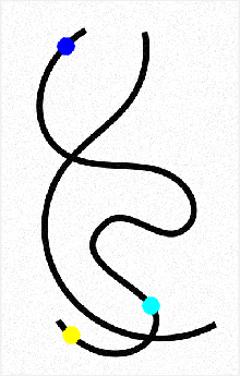
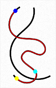
Adaptive anisotropy feature vector field. At a crossing point $\mathbf{x}$, each vector in the set $\mathfrak{M}_{\mathbf{x}}$ corresponds to a vessel direction. We need to choose the correct feature vector, i.e., the feature vector $\mathfrak{p}(\mathbf{x})$, for the target vessel from the set $\mathfrak{M}_{\mathbf{x}}$. Recall that the vector field $\mathfrak{p}$ is supposed to vary slowly along the the same structure. This means that we can seek $\mathfrak{p}(\mathbf{x})$ from the set $\mathfrak{M}_{\mathbf{x}}$ using a reference point $\mathbf{a}_{\mathbf{x}}$ which is close to $\mathbf{x}$, providing that $\mathfrak{p}(\mathbf{a}_{\mathbf{x}})$ has been known. Note that the detection of the reference points is presented in Section IV-B. In Fig. 4b, we denote the point $\mathbf{x}$ by a blue dot and its reference point $\mathbf{a}_{\mathbf{x}}$ by a red square. The cyan and yellow arrows at $\mathbf{x}$ (blue dot) represent the elements in the set $\mathfrak{M}_{\mathbf{x}}$ and the red arrow indicates the vector $\mathfrak{p}(\mathbf{a}_{\mathbf{x}})$.

Along the same tubular structure, the slow-varying property of the vector field $\mathfrak{p}$ in principle yields the maximal value of $|\langle\mathfrak{p}(\mathbf{x}),\mathfrak{p}(\mathbf{a}_{\mathbf{x}})\rangle|$ among all the elements in $\mathfrak{M}_{\mathbf{x}}$, i.e., $|\langle\mathfrak{p}(\mathbf{x}),\mathfrak{p}(\mathbf{a}_{\mathbf{x}})\rangle|\geq|\langle\mathbf{u},\mathfrak{p}(\mathbf{a}_{\mathbf{x}})\rangle|,\,\forall\mathbf{u}\in\mathfrak{M}_{\mathbf{x}}$. We define a set $\mathfrak{M}^{*}_{\mathbf{x}}\subseteq\mathfrak{M}_{\mathbf{x}}$ involving all the maximal feature vectors by

$$\mathfrak{M}^{*}_{\mathbf{x}}=\{\mathbf{w}\in\mathbb{R}^{2};~{}\mathbf{w}=\mathop{\arg\,\!\max}_{\mathbf{u}\in\mathfrak{M}_{\mathbf{x}}}|\langle\mathbf{u},\,\mathfrak{p}(\mathbf{a}_{\mathbf{x}})\rangle|\}.$$ (21)

Based on the set $\mathfrak{M}^{*}_{\mathbf{x}}$, the feature vector $\mathfrak{p}(\mathbf{x})$ can be identified by $\mathfrak{p}(\mathbf{x})=(\cos\mu(\mathbf{x}),\sin\mu(\mathbf{x}))^{T}$, where the orientation $\mu(\mathbf{x})\in\mathbb{S}^{1}$ is computed by

$$\mu(\mathbf{x})=\mathop{\arg\,\!\min}_{\theta:\mathfrak{g}(\theta)\in\mathfrak{M}^{*}_{\mathbf{x}}}|\Psi(\mathbf{x},\theta)-\Psi(\mathbf{a}_{\mathbf{x}},\mu(\mathbf{a}_{\mathbf{x}}))|.$$ (22)

In Fig. 4b, we show an example for the computation of $\mathfrak{p}(\mathbf{x})$, where the yellow arrow at $\mathbf{x}$ represents the identified vector $\mathfrak{p}(\mathbf{x})$ from the set $\mathfrak{M}_{\mathbf{x}}$. The vector field $\mathfrak{p}$ is constructed in a progressive way. The initialization for $\mathfrak{p}$ is set as $\mathfrak{p}(\mathbf{s})=(\cos\mu(\mathbf{s}),\sin\mu(\mathbf{s}))^{T}$, where $\mu(\mathbf{s})=\arg\max_{\theta}\Psi(\mathbf{s},\theta)$ and $\mathbf{s}$ is the source point. The progressive procedure for the computation of $\mathfrak{p}$ is carried out during the fast marching front propagation which is detailed in Section IV-B.

Appearance feature coherence penalty. Once the anisotropy feature vector $\mathfrak{p}(\mathbf{x})$ (or the corresponding orientation $\mu(\mathbf{x})$) is detected, we can compute the appearance feature coherence penalty $\phi_{\rm coh}$ based on the coherence-enhanced orientation score $\Psi$ (see Eq. (15)) and a new reference point $\mathbf{b}_{\mathbf{x}}$ by

$$\phi_{\rm coh}(\mathbf{x})=\exp\big{(}\lambda\,|\Psi(\mathbf{x},\mu(\mathbf{x}))-\Psi(\mathbf{b}_{\mathbf{x}},\mu(\mathbf{b}_{\mathbf{x}}))|\big{)},$$ (23)

where $\lambda$ is a positive constant. When the point $\mathbf{x}$ and its reference point $\mathbf{b}_{\mathbf{x}}$ are located at the same vessel, the value of $\phi_{\rm coh}(\mathbf{x})$ should be low according to the slow-varying prior for the appearance features.

Adaptively anisotropic tensor field. The anisotropic tubular minimal path model [44] uses $\mathcal{M}_{\rm scale}$ (see Eq. (5)) to compute the geodesic distances, which grow slowly along the directions $\hat{\mathfrak{q}}_{\rm of}(\cdot)$ inside the vessel regions. However, at some crossing point $\mathbf{x}$, the directions $\hat{\mathfrak{q}}_{\rm of}(\mathbf{x},\zeta_{\rm scale}(\mathbf{x}))$ from the OOF filter are not always proportional to the direction of the target vessel. This can be seen from Figs. 3a and 4a. In Fig. 4a, the direction of the target vessel at $\mathbf{x}$ (denoted by the blue dot) is indicated by a red line. The white line indicates $\hat{\mathfrak{q}}_{\rm of}(\mathbf{x},\zeta_{\rm scale}(\mathbf{x}))$ which is almost orthogonal to the red line. In order to get a metric with correct anisotropy enhancement, we consider a tensor field $T_{\rm aniso}$ formulated by

$$T_{\rm aniso}(\mathbf{x})=\xi_{\rm aniso}\,\mathfrak{p}^{\perp}(\mathbf{x})\otimes\mathfrak{p}^{\perp}(\mathbf{x}),$$ (24)

where $\xi_{\rm aniso}$ is a positive constant.

Finally, the term $T_{\rm base}$ in Eq. (19) is an image data-driven tensor field. It can be formulated in an isotropic form:

$$T_{\rm base}(\mathbf{x})=\exp(-\alpha\,\max_{\theta\in\mathbb{S}^{1}}\,\psi(\mathbf{x},\theta))\,\operatorname{I_{d}},$$ (25)

where $\operatorname{I_{d}}$ is the $2\times 2$ identity matrix and $\alpha\in\mathbb{R}^{+}$ is a constant. In order to take advantages of the anisotropy enhancement, we use the orientation score-based tensor field construction method [54] to build $T_{\rm base}$. This is done by replacing the identity matrix in Eq. (25) by a new tensor field $T^{-1}_{\rm os}$ which is the inverse of a positive definite symmetric tensor field $T_{\rm os}$

$$T_{\rm os}(\mathbf{x})=\frac{\int_{0}^{2\pi}\mathfrak{C}_{\mathbf{x}}(\theta)\Psi(\mathbf{x},\theta)\mathfrak{g}(\theta)\mathfrak{g}(\theta)^{T}d\theta}{\max\{\varepsilon_{2},\int_{0}^{2\pi}\mathfrak{C}_{\mathbf{x}}(\theta)d\theta\}}+\xi_{\rm ident}\operatorname{I_{d}},$$ (26)

where $\xi_{\rm ident}$ and $\varepsilon_{2}$ ($\varepsilon_{2}\approx 0$) are two small positive constants. The matrix $\xi_{\rm ident}\operatorname{I_{d}}$ ensures the non-singularity of the matrix $T_{\rm os}(\mathbf{x}),\,\forall\mathbf{x}\in\Omega$. Increasing the value of $\xi_{\rm ident}$ may reduce the anisotropy property of $T_{\rm os}(\mathbf{x})$. The desired tensor field $T_{\rm base}$ can be computed by

$$T_{\rm base}(\mathbf{x})=\exp(-\alpha\,\max_{\theta\in\mathbb{S}^{1}}\,\psi(\mathbf{x},\theta))\,T^{-1}_{\rm os}(\mathbf{x}),$$ (27)

where the parameter $\alpha\in\mathbb{R}^{+}$ controls the influence from the image data. At the crossing points, the tubular appearance and anisotropy features derived from both of the two overlapped structures will contribute to the tensor fields $T_{\rm os}$ and $T_{\rm base}$. In the following experiments, we make use of the tensor field $T_{\rm os}$ defined in Eq. (26) to build the tensor field $T_{\rm base}$.

Figure 5: (a) Two tubular structures crossing each other. The red dot indicates the source point. (b) Geodesic distances superimposed on the synthetic image. The green dot is the latest Accepted point $\mathbf{x}_{\rm min}$. (c) Close-up view of the region around $\mathbf{x}_{\rm min}$. The red square and the magenta dot are the reference points $\mathbf{a}$ and $\mathbf{b}$ respectively. The yellow line denotes the back-tracked short geodesic path.

IV Fast Marching Implementations

IV-A Fast Marching Fronts Propagation Scheme

In this section, we introduce the general scheme for the fast marching method which is first introduced in [31, 55]. It is an efficient way for the computation of the geodesic distances on the discretization domain $\mathbb{Z}^{2}$ of the image domain $\Omega$. Basically, the fast marching fronts visit all the grid points in a monotonically increasing order expanding from a set of source points, coupled with a course of label assignment operation through a map $\mathcal{V}:\mathbb{Z}^{2}\to\{$Far, Accepted, Front$\}$. One of the crucial point of the fast marching method is the neighbourhood system used. In contrast to the isotropic fast marching method [31] which invokes an 4-connectivity neighbourhood system, the anisotropic variant of the fast marching method [32] used in this paper requires a more complicated metric-dependent neighbourhood $\mathcal{S}$. It utilizes the geometry tool of the Lattice basis reduction and achieves an excellent balance between the complexity and accuracy for the geodesic distance computation. For the sake of simplicity, we define an inverse neighbourhood $\mathcal{S}^{-1}$ for each grid point $\mathbf{x}\in\mathbb{Z}^{2}$ such that $\mathcal{S}^{-1}(\mathbf{x}):=\{\mathbf{z}\in\mathbb{Z}^{2};\mathbf{x}\in\mathcal{S}(\mathbf{z})\}$. Thus a grid point $\mathbf{y}\in\mathbb{Z}^{2}$ is a neighbour point of $\mathbf{x}$ if $\mathbf{y}\in\mathcal{S}^{-1}(\mathbf{x})$. We refer to [32, 33] for more details on $\mathcal{S}$ and $\mathcal{S}^{-1}$.

Let $\mathcal{U}_{\mathbf{s}}:\mathbb{Z}^{2}\backslash\{\mathbf{s}\}\to\mathbb{R}^{+}_{0}$ be the geodesic distance map associated to the metric $\mathcal{F}_{\rm coh}$ defined in (18), where $\mathbf{s}\in\mathbb{Z}^{2}$ is the source point such that $\mathcal{U}_{\mathbf{s}}(\mathbf{s})=0$. In each geodesic distance update iteration, a point $\mathbf{x}_{\rm min}\in\mathbb{Z}^{2}$ with minimal $\mathcal{U}_{\mathbf{s}}$ among all the Front points can be detected by

$$\mathbf{x}_{\rm min}=\mathop{\arg\,\!\min}_{\mathbf{x}:\mathcal{V}(\mathbf{x})=\emph{Front}}\mathcal{U}_{\mathbf{s}}(\mathbf{x}).$$ (28)

The point $\mathbf{x}_{\rm min}$ is immediately tagged as Accepted. In the following, $\mathbf{x}_{\rm min}$ is called the latest Accepted point. The geodesic distances for all the neighbour points $\mathbf{x}_{\rm n}\in\mathcal{S}^{-1}(\mathbf{x}_{\rm min})$ with $\mathcal{V}(\mathbf{x}_{\rm n})\neq$Accepted can be estimated by the solution to the Hopf-Lax operator [32]

$$\mathcal{U}_{\mathbf{s}}(\mathbf{x}_{\rm n})=\min_{\mathbf{z}\in\partial\mathcal{S}(\mathbf{x}_{\rm n})}\{\mathcal{F}_{\rm coh}(\mathbf{x}_{\rm n},\mathbf{z}-\mathbf{x}_{\rm n})+\operatorname{I}_{\mathcal{S}(\mathbf{x}_{\rm n})}\mathcal{U}_{\mathbf{s}}(\mathbf{z})\}$$ (29)

where $\operatorname{I}_{\mathcal{S}(\cdot)}$ is a piecewise linear interpolator and $\operatorname{I}_{\mathcal{S}(\mathbf{x}_{\rm n})}\mathcal{U}_{\mathbf{s}}(\mathbf{z})$ is a distance value estimated by the interpolator $\operatorname{I}_{\mathcal{S}(\mathbf{x}_{\rm n})}$ in the neighbourhood $\mathcal{S}(\mathbf{x}_{\rm n})$. The Hopf-Lax operator in Eq. (29) is an approximation to the Eikonal equation based on Bellman’s optimality principle.

IV-B Single Front Propagation Implementation

In this section, we present the method for updating the metric $\mathcal{F}_{\rm coh}$ in conjunction with the detected reference points. This is done by the fast marching front propagation scheme [32] and a truncated geodesic curve back-tracking scheme [51]. Since the metric $\mathcal{F}_{\rm coh}$ is constructed during the front propagation, we refer to $\mathcal{F}_{\rm coh}$ as a dynamic Riemannian metric.

In each geodesic distance update iteration, we first search for the latest Accepted point $\mathbf{x}_{\rm min}$ from all the Front points. In Fig. 5b, we take a green dot as an example for such a point $\mathbf{x}_{\rm min}$. From $\mathbf{x}_{\rm min}$ we can track a geodesic path $\bar{\mathcal{C}}_{\mathbf{x}_{\rm min}}$ by solving the following gradient descent ODE on $\mathcal{U}_{\mathbf{s}}$

$$\bar{\mathcal{C}}^{\prime}_{\mathbf{x}_{\rm min}}(v)=-\frac{\mathcal{T}^{-1}_{\rm coh}(\bar{\mathcal{C}}_{\mathbf{x}_{\rm min}}(v))\nabla\mathcal{U}_{\mathbf{s}}(\bar{\mathcal{C}}_{\mathbf{x}_{\rm min}}(v))}{\|\mathcal{T}^{-1}_{\rm coh}(\bar{\mathcal{C}}_{\mathbf{x}_{\rm min}}(v))\nabla\mathcal{U}_{\mathbf{s}}(\bar{\mathcal{C}}_{\mathbf{x}_{\rm min}}(v))\|},$$ (30)

with $\bar{\mathcal{C}}_{\mathbf{x}_{\rm min}}(0)=\mathbf{x}_{\rm min}$ and $\bar{\mathcal{C}}_{\mathbf{x}_{\rm min}}(L)=\mathbf{s}$, where $L$ is the Euclidean curve length of $\bar{\mathcal{C}}_{\mathbf{x}_{\rm min}}$. Since each neighbour point $\mathbf{x}_{\rm n}\in\mathcal{S}^{-1}(\mathbf{x}_{\rm min})$ is close to $\mathbf{x}_{\rm min}$, we can seek the reference points $\mathbf{a}_{\mathbf{x}_{\rm n}}$ and $\mathbf{b}_{\mathbf{x}_{\rm n}}$ for the points $\mathbf{x}_{\rm n}$ with $\mathcal{V}(\mathbf{x}_{\rm n})\neq$Accepted through the geodesic path $\bar{\mathcal{C}}_{\mathbf{x}_{\rm min}}$ as follows:

$$\mathbf{a}_{\mathbf{x}_{\rm n}}=\bar{\mathcal{C}}_{\mathbf{x}_{\rm min}}(u_{1}),\quad\mathbf{b}_{\mathbf{x}_{\rm n}}=\bar{\mathcal{C}}_{\mathbf{x}_{\rm min}}(u_{2}),$$ (31)

where $u_{1},\,u_{2}\in(0,L)$ are two positive constants and $u_{1}\leq u_{2}$. In this case, in each distance update iteration, all the non-accepted neighbour points $\mathbf{x}_{\rm n}$ of $\mathbf{x}_{\rm min}$ share the same reference points. Henceforth we respectively denote by $\mathbf{a}$ and $\mathbf{b}$ the reference points $\mathbf{a}_{\mathbf{x}_{\rm n}}$ and $\mathbf{b}_{\mathbf{x}_{\rm n}}$ for simplicity. In Fig. 5c, the portion of the geodesic path $\bar{\mathcal{C}}_{\rm\mathbf{x}_{\rm min}}$ between $\mathbf{x}_{\rm min}$ (green dot) and the reference point $\mathbf{a}$ (red square) is illustrated by a yellow line. The reference points $\mathbf{a}$ and $\mathbf{b}$ for all the non-accepted neighbour points $\mathbf{x}_{\rm n}$ are respectively denoted by a red square and a magenta dot.

The fast marching front propagation scheme provides a progressive way to identify the reference points, which can be used to update the metric $\mathcal{F}_{\rm coh}$. The details are illustrated in Algorithm 1. In practice, the reference points are detected via two thresholding values $\chi_{1},\,\chi_{2}$ with $\chi_{1}\leq\chi_{2}$, which denote the numbers of grid points passed through by each back-tracked geodesic. This tracking processing is terminated once the reference point corresponding to the larger thresholding value $\chi_{2}$ is obtained or the source point is reached.

Figure 6: (a)-(b): Control sets $\mathcal{B}_{\rm aniso}(\mathbf{x}_{\rm min})$ and $\mathcal{B}_{\rm coh}(\mathbf{x}_{\rm min})$ derived from the picture in Fig. 5a, where $\mathbf{x}_{\rm min}$ is indicated by the green dot in Fig. 5b. In each figure, the black line indicates the direction of the major axis of the corresponding ellipse while the red line indicates the direction of the target vessel shown in Fig. 5a at the crossing point.

Figure 7: (a) The geodesic distance map $\mathcal{U}_{\mathbf{s}}$ superimposed on the retinal patch. The black line indicates the geodesic curve $\mathcal{C}_{\mathfrak{m},\mathbf{s}}$ and the red dot is the point $\mathbf{s}$. The green dot indicates the saddle point $\mathfrak{m}$. (b) The geodesic distance map $\mathcal{U}_{\mathbf{q}}$. The black line denotes $\mathcal{C}_{\mathfrak{m},\mathbf{q}}$ and the yellow dot indicates $\mathbf{q}$. (c) The white line denotes the concatenated curve $\mathcal{C}_{\mathbf{s},\mathbf{q}}$. The blue shadow region is the constrained region $\mathbb{U}$. (d) The radius-lifted geodesic curve $\hat{\mathcal{C}}_{\hat{\mathbf{s}},\hat{\mathbf{q}}}$.

Metric visualization. We use the control set, a tool for visualizing the anisotropy of a metric, to show the advantages of the proposed metric $\mathcal{F}_{\rm coh}$ at a crossing point. For the metric $\mathcal{F}_{\rm coh}$ at a point $\mathbf{x}$, it can be defined by

$$\mathcal{B}_{\rm coh}(\mathbf{x})=\{\mathbf{u}\in\mathbb{R}^{2};~{}\mathcal{F}_{\rm coh}(\mathbf{x},\mathbf{u})\leq 1\}.$$ (32)

For comparison, we also consider an anisotropic metric

$$\tilde{\mathcal{F}}_{\rm aniso}(\mathbf{x},\mathbf{u})=\sqrt{\langle\mathbf{u},\mathcal{M}_{\rm aniso}(\mathbf{x},\zeta_{\rm scale}(\mathbf{x}))\mathbf{u}\rangle},$$

where $\mathcal{M}_{\rm aniso}$ is defined in Eq. (II-B). Let $\mathcal{B}_{\rm aniso}$ be the control set of $\tilde{\mathcal{F}}_{\rm aniso}$ constructed through Eq. (32). For a Riemannian metric, the control set appears to be an ellipse and we expect that the direction of its major axis should align with the vessel direction as much as possible.

We construct the metrics $\tilde{\mathcal{F}}_{\rm aniso}$ and $\mathcal{F}_{\rm coh}$ for the synthetic image shown in Fig. 4a. We illustrate the control sets $\mathcal{B}_{\rm aniso}(\mathbf{x}_{\rm min})$ and $\mathcal{B}_{\rm coh}(\mathbf{x}_{\rm min})$ respectively in Figs. 6a and 6b, where the point $\mathbf{x}_{\rm min}$ is indicated by the green dot in Fig. 5b. The red line in each figure indicates the target vessel direction at $\mathbf{x}_{\rm min}$ while each black line indicates the major axis of the corresponding ellipse. One can point out that in Fig. 6a, the black and red lines are misaligned with each other since the tensor $\mathcal{M}_{\rm aniso}(\mathbf{x}_{\rm min})$ is dominated by the strong vessel. While in Fig. 6b, the red and black lines are almost collinear to each other thanks to the adaptive anisotropic tensor $T_{\rm aniso}(\mathbf{x}_{\rm min})$.

Algorithm 1 Single Front Propagation Scheme

The orientation score $\Psi$, the points $\mathbf{s}$ and $\mathbf{q}$.

Geodesic distance map $\mathcal{U}_{\mathbf{s}}$.

$\bullet$ Set $\mathcal{U}_{\mathbf{s}}(\mathbf{x})\leftarrow\infty$ and $\mathcal{V}(\mathbf{x})\leftarrow$ Far, $\forall\mathbf{x}\in\Omega\backslash\{\mathbf{s}\}$.

$\bullet$ Set $\mathcal{U}_{\mathbf{s}}(\mathbf{s})\leftarrow 0,\mathcal{V}(\mathbf{s})\leftarrow$ Front, $\mathfrak{p}(\mathbf{s})\leftarrow\arg\max_{\theta}\Psi(\mathbf{s},\theta)$.

1:while $\mathcal{V}(\mathbf{q})\neq$Accepted do

2:     Find $\mathbf{x}_{\rm min}$, the Front point which minimizes $\mathcal{U}_{\mathbf{s}}$.

3:     Set $\mathcal{V}(\mathbf{x}_{\rm min})\leftarrow$ Accepted.

4:     Find the reference points $\mathbf{a}$ and $\mathbf{b}$ through Eq. (31).

5:     for All $\mathbf{x}_{\rm n}\in\mathcal{S}^{-1}(\mathbf{x}_{\rm min})$ and $\mathcal{V}(\mathbf{x}_{\rm n})\neq$ Accepted do

6:         Set $\mathcal{V}(\mathbf{x}_{\rm n})\leftarrow$ Front.

7:         Update $\mathfrak{p}(\mathbf{x}_{\rm n})$ by the reference point $\mathbf{a}$ via Eq. (22).

8:         Update $T_{\rm coh}(\mathbf{x}_{\rm n})$ by the point $\mathbf{b}$ via Eq. (19).

9:         Estimate $\mathcal{U}_{\rm tem}(\mathbf{x}_{\rm n})$ by evaluating the Hopf-Lax operator in Eq. (29).

10:         Set $\mathcal{U}_{\mathbf{s}}(\mathbf{x}_{\rm n})\leftarrow\min\{\mathcal{U}_{\rm tem}(\mathbf{x}_{\rm n}),\mathcal{U}_{\mathbf{s}}(\mathbf{x}_{\rm n})\}$.

11:     end for

12:end while

IV-C Partial Fronts Propagation Implementation

In the single front propagation scheme presented in Section IV-B, in each geodesic distance update iteration, the back-tracked geodesic path $\bar{\mathcal{C}}_{\mathbf{x}_{\rm min}}$ obtained from Eq. (30) always links the latest accepted point $\mathbf{x}_{\rm min}$ to the source point $\mathbf{s}$. When the fast marching front arrives closely to the end point $\mathbf{q}$, we expect that the associated reference points are located at the vessel segment between $\mathbf{x}_{\rm min}$ and $\mathbf{q}$ in order to obtain more adequate appearance coherence penalty. For this purpose, we consider the partial fronts propagation method [42].

We can estimate the respective geodesic distance maps $\mathcal{U}_{\mathbf{s}}$ and $\mathcal{U}_{\mathbf{q}}$ with $\mathcal{U}_{\mathbf{s}}(\mathbf{s})=\mathcal{U}_{\mathbf{q}}(\mathbf{q})=0$ through the fast marching method with dynamic metric update scheme as presented in Algorithm 1. A saddle point $\mathfrak{m}$ is the point which has the minimal value of $\mathcal{U}_{\mathbf{s}}$ (or $\mathcal{U}_{\mathbf{q}}$) among the equivalence distance point set $\mathscr{A}=\{\mathbf{x};\,\mathcal{U}_{\mathbf{s}}(\mathbf{x})=\mathcal{U}_{\mathbf{q}}(\mathbf{x})\}$, i.e.,

$$\mathfrak{m}=\mathop{\arg\,\!\min}_{\mathbf{x}\in\mathscr{A}}\,\mathcal{U}_{\mathbf{s}}(\mathbf{x}).$$ (33)

We can track two geodesic curves $\bar{\mathcal{C}}_{\mathfrak{m},\mathbf{s}}$ and $\bar{\mathcal{C}}_{\mathfrak{m},\mathbf{q}}$ from the saddle point $\mathfrak{m}$ through the solutions to the gradient descent ODEs respectively on $\mathcal{U}_{\mathbf{s}}$ and $\mathcal{U}_{\mathbf{q}}$. Let $\mathcal{C}_{\mathbf{s},\mathfrak{m}},\,\mathcal{C}_{\mathbf{q},\mathfrak{m}}\in\mathfrak{L}([0,1],\Omega)$ be the reversed and re-parameterized curves of $\bar{\mathcal{C}}_{\mathfrak{m},\mathbf{s}}$ and $\bar{\mathcal{C}}_{\mathfrak{m},\mathbf{q}}$ respectively. The final geodesic curve $\mathcal{C}_{\mathbf{s},\mathbf{q}}$ with $\mathcal{C}_{\mathbf{s},\mathbf{q}}(0)=\mathbf{s}$ and $\mathcal{C}_{\mathbf{s},\mathbf{q}}(1)=\mathbf{q}$ can be obtained by concatenating the geodesic curves $\mathcal{C}_{\mathfrak{m},\mathbf{s}}$ and $\mathcal{C}_{\mathfrak{m},\mathbf{q}}$ as follows:

$$\mathcal{C}_{\mathbf{s},\mathbf{q}}(v)=\begin{cases}\mathcal{C}_{\mathbf{s},\mathfrak{m}}(2v),\quad&\text{if~{}}0\leq v\leq 1/2,\\ \mathcal{C}_{\mathbf{q},\mathfrak{m}}(2(1-v)),\quad&\text{if~{}}1/2<v\leq 1.\end{cases}$$ (34)

For numerical implementation, we perform the fast marching front propagation as presented in Algorithm 1 simultaneously from the points $\mathbf{s}$ and $\mathbf{q}$. In this case, the saddle point $\mathfrak{m}$ is the first meeting point of the two fronts respectively expanding from $\mathbf{s}$ and $\mathbf{q}$. That partial fronts propagation will be terminated once the saddle point $\mathfrak{m}$ is detected in order to reduce the computation complexity. We illustrate an example for this partial fronts propagation scheme in Fig. 7. In Figs. 7a and 7b, the geodesic distance maps $\mathcal{U}_{\mathbf{s}}$ and $\mathcal{U}_{\mathbf{q}}$ together with the corresponding geodesic paths $\bar{\mathcal{C}}_{\mathfrak{m},\mathbf{s}}$ and $\bar{\mathcal{C}}_{\mathfrak{m},\mathbf{q}}$ are demonstrated. The white line in Fig. 7c indicates the concatenated curve $\mathcal{C}_{\mathbf{s},\mathbf{q}}$.

IV-D Region-Constrained Radius-lifted Geodesic Model

The geodesic curves associated to the metric $\mathcal{F}_{\rm coh}$ are computed in the image domain $\Omega$. However, for a complete tubular structure segmentation, the goal is to search for the centerline and the corresponding thickness of the vessel simultaneously. Moreover, we observe that the geodesic curves from $\mathcal{F}_{\rm coh}$ sometimes suffer from a centerline bias problem, mainly because of the inhomogeneous intensity distributions. To solve these problems, we propose a region-constrained minimal path method, providing that a prescribed curve is given in order to build the constrained region.

We take the concatenated curve $\mathcal{C}_{\mathbf{s},\mathbf{q}}$ as an example of the prior curve. Let $\mathbb{U}\subset\Omega$ be a bounded and connected tubular neighbourhood of $\mathcal{C}_{\mathbf{s},\mathbf{q}}$ (see Fig. 7c for an example of $\mathbb{U}$), which can be efficiently computed by the morphological dilation operator. The region-constrained metric $\mathcal{F}_{\rm cstr}:\hat{\Omega}\to[0,\infty]$ can be expressed for any point $\hat{\mathbf{x}}=(\mathbf{x},r)$ by

$$\mathcal{F}_{\rm cstr}(\hat{\mathbf{x}},\hat{\mathbf{u}})=\begin{cases}\|\hat{\mathbf{u}}\|_{\mathcal{M}_{\rm scale}(\hat{\mathbf{x}})},&\forall\mathbf{x}\in\mathbb{U},\\ \infty,&\text{otherwise},\end{cases}$$ (35)

where $\mathcal{M}_{\rm scale}$ is defined in Eq. (5). The geodesic distance map associated to $\mathcal{F}_{\rm cstr}$ can be efficiently solved by the general anisotropic variant of the fast marching method [32], where the propagation is terminated once the end point $\hat{\mathbf{q}}=(\mathbf{q},\zeta_{\rm scale}(\mathbf{q}))$ is tagged as Accepted. Obviously, the radius-lifted geodesic curve $\hat{\mathcal{C}}_{\hat{\mathbf{s}},\hat{\mathbf{q}}}=(\eta,\tau)$ associated to $\mathcal{F}_{\rm cstr}$ satisfies $\eta(u)\in\mathbb{U},\,\forall u\in[0,1]$. We show the geodesic curve $\hat{\mathcal{C}}_{\hat{\mathbf{s}},\hat{\mathbf{q}}}$ in Fig. 7d, where the red curve denotes the centerline $\eta$ and the yellow contour depicts the vessel boundary derived from $\tau$.

The region-constrained minimal path model can seek a complete vessel segmentation in conjunction with the appearance feature coherence-penalized minimal path model. In the following experiments, we take the paths from the metric $\mathcal{F}_{\rm coh}$ as the prior curves to establish the respective tubular regions for the metric $\mathcal{F}_{\rm cstr}$.

Remark. The region-constrained minimal path model can be taken as an efficient way to estimate the vessel thickness measurement from a binary vessel segmentation map. An interesting example as introduced in [56] is to generate a set of disjoint skeletons from the binary segmentation map. As a result, each skeleton can provide two end points and a tubular region for $\mathcal{F}_{\rm cstr}$, yielding the thickness measurement for each vessel segment.

V Experimental Results

V-A Parameter Setting

The orientation score $\Psi$ is computed by the oriented Gaussian kernels defined in Eq. (13). In numerical implementations, the variances $\sigma_{1},\,\sigma_{2}$ of the oriented Gaussian kernels dominate the anisotropy properties of these kernels. In the experiments, we fix $\sigma_{1}=300$ and $\sigma_{2}=1$ to construct a series of well-oriented Gaussian kernels. The parameter $w$ which controls the size of the truncated window for each oriented Gaussian kernel should depend on the image data. For instance, if the target tubular structure has strong tortuosity, the values of $w$ should be small. In case the target vessel crosses a stronger and thicker one, especially when the target is invisible at the crossing region, a large value of $w$ is preferred. In our experiments, we set $w=11$ unless specified otherwise. The thresholding lengths $\chi_{1}$ and $\chi_{2}$ (in grid point) of the back-tracked short geodesic curves are used to seek the two reference points. The parameter $\chi_{1}$ contributes to the estimation of the vector field $\mathfrak{p}$ based on the Eqs. (21) and (22). When the target has strong tortuosity, the reference point associated to $\chi_{1}$ should be close to the latest Accepted point, which corresponds to a small $\chi_{1}$. The values of $\chi_{2}$ affect the appearance feature coherence penalty, which should be set dependently to the image data. In default, we experimentally set $\chi_{1}=1$ and $\chi_{2}=12$. The parameters $\alpha$ in Eq. (27) and $\lambda$ in Eq. (23) control the influence from the tubular appearance and from the coherence penalty, respectively. For the case that a weak tubular structure crosses a strong one, the values of $\alpha$ should be low while the values of $\lambda$ should be high. Finally, the constants $\xi_{\rm ident}$ and $\xi_{\rm aniso}$ used in Eqs. (26) and (24) dominates the anisotropy property of the tensor fields $T_{\rm base}$ and $T_{\rm aniso}$. We declare the default values for these parameters as follows: $\alpha=2$, $\lambda=20$, $\xi_{\rm aniso}=10$ and $\xi_{\rm ident}=0.1$. In the following experiments, we make use of the default setting discussed above unless specified otherwise. The experiments are performed on a standard Intel Core i$7$ of $4.2$GHz architecture with $32$Gb RAM.

Figure 8: Comparative results on a synthetic image. Left Prescribed points. Right Geodesic paths obtained from the metrics $\mathcal{F}_{\rm aniso}$ (blue dash line), $\mathcal{F}_{\rm e}$ (green solid line) and $\mathcal{F}_{\rm coh}$ (red line). The objective is to extract the weak tubular structure.

Figure 9: Comparative results on retinal images. Column 1 Prescribed points which are indicated by dots. Columns 2-4 Minimal paths from the metrics of $\mathcal{F}_{\rm aniso}$, $\mathcal{F}_{\rm e}$, the proposed $\mathcal{F}_{\rm coh}$ and $\mathcal{F}_{\rm cstr}$, respectively. Note that we only show the centerline positions of the minimal paths from the RLAR metric $\mathcal{F}_{\rm aniso}$.

Figure 10: Comparative results on retinal images with strong tortuosity. Column 1 Prescribed points indicated by dots. Columns 2-4 Minimal paths from the RLAR metric $\mathcal{F}_{\rm aniso}$, the FE metric $\mathcal{F}_{\rm e}$ and the proposed AFC metric $\mathcal{F}_{\rm coh}$ respectively.

Figure 11: Comparative results on neural fibre images. Column 1 Prescribed source and end points indicated by blue and yellow dots. Columns 2-4 Minimal paths (indicated by red lines) derived from the metrics of $\mathcal{F}_{\rm aniso}$, $\mathcal{F}_{\rm e}$ and $\mathcal{F}_{\rm coh}$, respectively.

Figure 12: Comparative results on a leaf image. (a) The leaf image with source point (blue dots) and end points (yellow dots). (b)-(e): Geodesic curves from the metrics $\mathcal{F}_{\rm aniso}$, $\mathcal{F}_{\rm e}$, $\mathcal{F}_{\rm coh}$ and $\mathcal{F}_{\rm cstr}$ respectively.

V-B Comparative Results with State-of-the-art Metrics

We compare the proposed metrics, including the appearance feature coherence penalized (AFC) metric $\mathcal{F}_{\rm coh}$ and the region-constrained (RC) metric $\mathcal{F}_{\rm cstr}$, to the radius-lifted anisotropic Riemannian (RLAR) metric [44] and the Finsler elastica (FE) metric [46]. By the tensor field $\mathcal{M}_{\rm scale}$ in Eq. (5), the RLAR metric $\mathcal{F}_{\rm aniso}:\hat{\Omega}\to[0,\infty]$ can be formulated by

$$\mathcal{F}_{\rm aniso}(\hat{\mathbf{x}},\hat{\mathbf{u}})=\|\hat{\mathbf{u}}\|_{\mathcal{M}_{\rm scale}(\hat{\mathbf{x}})}.$$ (36)

The anisotropy ratio [44] for $\mathcal{F}_{\rm aniso}$ can be defined by

$$C_{\rm ratio}(\mathcal{F}_{\rm aniso})=\max_{\hat{\mathbf{x}}\in\Omega}\left\{\max_{\|\mathbf{u}_{1}\|=\|\mathbf{u}_{2}\|=1}\frac{\|\mathbf{u}_{1}\|_{\mathcal{M}_{\rm aniso}(\hat{\mathbf{x}})}}{\|\mathbf{u}_{2}\|_{\mathcal{M}_{\rm aniso}(\hat{\mathbf{x}})}}\right\},$$

where $\mathcal{M}_{\rm aniso}$ is defined in Eq. (II-B). The values of the parameter $\alpha_{\rm aniso}$ (see Eq. (II-B)) can be determined by the ratio $C_{\rm ratio}$. We set $C_{\rm ratio}=10$ in the following experiments. The computation of the geodesic distance associated with $\mathcal{F}_{\rm aniso}$ will be terminated once all the end points have been reached.

The FE metric $F_{\rm e}:\Omega\times\mathbb{S}^{1}\to[0,\infty]$ is established in an orientation-lifted space [46], which can be expressed by

$$\mathcal{F}_{\rm e}(\tilde{\mathbf{x}},\tilde{\mathbf{u}})=P_{\rm os}(\tilde{\mathbf{x}})(\sqrt{\rho^{2}\|\mathbf{u}\|^{2}+2\rho\beta_{\rm ela}|\nu|^{2}}-(\rho-1)\langle\mathfrak{g}(\theta),\mathbf{u}\rangle)$$

where $\tilde{\mathbf{x}}=(\mathbf{x},\theta)\in\Omega\times\mathbb{S}^{1}$ is an orientation-lifted point and $\tilde{\mathbf{u}}=(\mathbf{u},\nu)\in\mathbb{R}^{3}$ is a vector. The value of the parameter $\rho$ determining the anisotropy and asymmetry properties of the metric $\mathcal{F}_{\rm e}$ is fixed to $100$ for all the experiments. The function $P_{\rm os}:\Omega\times\mathbb{S}^{1}\to\mathbb{R}^{+}$ can be derived from the orientation score $\psi$ defined in Eq. (14), i.e.,

$$P_{\rm os}(\mathbf{x},\theta)=\exp(-\alpha_{\rm ela}\,\psi(\mathbf{x},\theta)/\|\psi\|_{\infty}),\quad\alpha_{\rm ela}\in\mathbb{R}^{+}.$$

The values of $\alpha_{\rm ela}$ and $\beta_{\rm ela}\in\mathbb{R}^{+}$ control the balance between the curvature penalization and the image data [46], which should be tuned dependently on the target structures. In our experiments, we adopt the same Eikonal solver as used in [46], i.e., the Finsler variant of the fast marching method [33], for the FE metric $\mathcal{F}_{\rm e}$. We also use the same tubular structure extraction strategy as proposed in [46].

In Fig. 8, we compare the proposed AFC metric $\mathcal{F}_{\rm coh}$ with the RLAR metric $\mathcal{F}_{\rm aniso}$ and the FE metric $\mathcal{F}_{\rm e}$. The structure in Fig. 8 is comprised of a strong tubular segment and a weak one. The goal is to extract the weak structure between two points. Both the minimal paths from $\mathcal{F}_{\rm aniso}$ (blue dash line) and $\mathcal{F}_{\rm e}$ (green solid line) prefer to pass through the tubular segment with strong appearance features. In contrast, the geodesic curve (red line) associated to $\mathcal{F}_{\rm coh}$ can delineate the desired structure. In this experiment, we use the default parameters for $\mathcal{F}_{\rm coh}$ except for $\chi_{2}$ which is set to $15$.

In Fig. 9, the minimal paths derived from the RLAR metric $\mathcal{F}_{\rm aniso}$, the FE metric $\mathcal{F}_{\rm e}$, the AFC metric $\mathcal{F}_{\rm coh}$ and the RC metric $\mathcal{F}_{\rm cstr}$ are shown in columns $2$ to $5$ respectively. In the first column, the prescribed points are indicated by the green and yellow dots. In column $2$, the geodesic paths yielded by the RLAR metric $\mathcal{F}_{\rm aniso}$ suffered from the short branches combination problem, where these paths prefer to pass through the vessel segments with strong appearance features. In the first three rows of column $3$, we also observe the short branches combination problem for the geodesic paths from the FE metric $\mathcal{F}_{\rm e}$. In column $4$, the geodesic paths from the AFC metric $\mathcal{F}_{\rm coh}$ can correctly depict the desired vessel segments due to the appearance feature coherence penalization. In column $5$, we illustrate the radius-lifted minimal paths where the yellow contours delineate the vessel boundaries and the red curves indicate the vessel centerlines. One can claim that the geodesic paths in column $5$ is capable of accurately describing the target vessels. In rows $1$ to $3$, we use the default parameters for the metric $\mathcal{F}_{\rm coh}$. While in row $4$, we set $\lambda=10$.

In some extent, the short branches combination problem can be solved by the FE metric $\mathcal{F}_{\rm e}$, as shown in column $3$ and row $4$ of Fig. 9. However, it is difficult for the FE metric to get the accurate results in the situation of extracting a weak vessel with strong tortuosity especially when the target is close to another vessel with strong appearance features. We show two such examples in Fig. 10. In columns $2$ to $4$ of Fig. 10, the results from the RLAR metric $\mathcal{F}_{\rm aniso}$, the FE metric $\mathcal{F}_{\rm e}$ and the RC metric $\mathcal{F}_{\rm cstr}$ are shown, indicating that only the proposed metric $\mathcal{F}_{\rm cstr}$ can get the expected paths.

In Fig. 11 we show the results from the RLAR metric $\mathcal{F}_{\rm aniso}$, the FE metric $\mathcal{F}_{\rm e}$ and the AFC metric $\mathcal{F}_{\rm coh}$ on two neural fibre images. The curvilinear structures are treated as thin vessels. Some portions of the targets between the blue and yellow dots are weakly defined. Both the metrics $\mathcal{F}_{\rm aniso}$ and $\mathcal{F}_{\rm e}$ fail to detect the expected structures, while the minimal paths from the metric $\mathcal{F}_{\rm coh}$ are able to accurately depict the targets. In this experiment, we use the default parameters for the metric $\mathcal{F}_{\rm coh}$ except for $\chi_{2}$ which is set to $5$. The parameters $\alpha_{\rm ela}$ and $\beta_{\rm ela}$ for the FE metric $\mathcal{F}_{\rm e}$ are set to $3$ and $50$ respectively.

In Fig. 12 we show the geodesic paths on a leaf image [57] with respect to the metrics $\mathcal{F}_{\rm aniso}$, $\mathcal{F}_{\rm e}$, $\mathcal{F}_{\rm coh}$ and $\mathcal{F}_{\rm cstr}$. The geodesic paths shown in Fig. 12b from the RLAR metric $\mathcal{F}_{\rm aniso}$ fail to detect the left vein. In Figs. 12c, 12d and 12e, the geodesic paths derived from the metrics $\mathcal{F}_{\rm e}$, $\mathcal{F}_{\rm coh}$ and $\mathcal{F}_{\rm cstr}$ are able to obtain the desired results. However, the computation time associated to the metric $\mathcal{F}_{\rm e}$ in Fig 12c requires about $77$ seconds for the leaf image of size $548\times 1447$, while the computation time in Fig 12d is only around $8$ seconds involving the construction of $T_{\rm base}$ in Eq. (27) and the geodesic distance computation. Note that for the results in Fig. 12e, we only show the centerline positions denoted by the first two coordinates in each $3$D point in the obtained geodesic path. In this experiment, we use the single front propagation scheme for the results in Fig. 12d.

TABLE I: Quantitative comparisons of different metrics on DRIVE.

$\mathbb{A}$		$\mathcal{F}_{\rm aniso}$	$\mathcal{F}_{\rm e}$	$\mathcal{F}_{\rm coh}$	$\mathcal{F}_{\rm cstr}$
Artery Region	Avg.	0.36	0.65	0.92	0.98
	Max.	1	1	1	1
	Min.	0.02	0.13	0.60	0.79
	Std.	0.26	0.29	0.08	0.04
Dilated Skeleton	Avg.	0.32	0.53	0.76	0.90
	Max.	0.95	0.94	0.93	0.99
	Min.	0.02	0.12	0.35	0.5
	Std.	0.25	0.25	0.12	0.08

TABLE II: Quantitative comparisons of different metrics on IOSTAR.

$\mathbb{A}$		$\mathcal{F}_{\rm aniso}$	$\mathcal{F}_{\rm e}$	$\mathcal{F}_{\rm coh}$	$\mathcal{F}_{\rm cstr}$
Dilated Artery Region	Avg.	0.52	0.78	0.93	0.95
	Max.	0.99	1	1	1
	Min.	0.03	0.03	0.53	0.54
	Std.	0.34	0.33	0.08	0.08

V-C Quantitative Comparative Results

In this section, we quantitatively compare the vessel detection performance of the proposed metrics $\mathcal{F}_{\rm coh}$ and $\mathcal{F}_{\rm cstr}$ with $\mathcal{F}_{\rm aniso}$ and $\mathcal{F}_{\rm e}$ on $88$ patches of retinal images from the DRIVE and IOSTAR datasets. The corresponding artery-vein (A-V) labeled images of the DRIVE and IOSTAR datasets are provided by [59] and [26], respectively. Each patch includes a retinal artery which is close to or crosses a vein with stronger appearance features. The objective is to extract the artery centerline between two given points.

Let $\mathbb{A}$ be the set of the grid points inside the target artery region derived from the respective A-V label image and let $|\mathbb{A}|$ be the number of elements of the set $\mathbb{A}$. In addition, we define a set $\Gamma$ of grid points passed through by a continuous geodesic curve. A scalar-valued measure $\Theta\in[0,1]$ can be defined by $\Theta=|\Gamma\cap\mathbb{A}|/|\Gamma|$.

For the DRIVE dataset, we provide two ways to construct the set $\mathbb{A}$ from the A-V labeled images. The first way is to regard $\mathbb{A}$ as the set of all the grid points tagged as artery. The second way is to skeletonize the regions labeled as artery via the morphological operators, followed by a dilation operation with radius $1$ on these skeletons. Then we remove the non-vessel grid points from the dilated skeletons. In Table. I, the two construction methods are referred to as Artery Region and Dilated Skeleton respectively. For the IOSTAR dataset, we directly dilate the regions tagged as artery by a morphological operator with radius $1$, which is named Dilated Artery Region. The use of the dilation operator is to mitigate the influences from the strong intensity inhomogeneities of the images in IOSTAR dataset. The results from $\mathcal{F}_{\rm coh}$ shown in Table I are obtained using the default parameters described in Section V-A. In Table II, $\alpha$ and $\lambda$ for the metric $\mathcal{F}_{\rm coh}$ are chosen from the sets $\{1,2,3\}$ and $\{10,20,30\}$, respectively to mitigate the effects from the retinal vessel centre reflection. The quantitively comparative results on the DRIVE and IOSTAR datasets associated to the metrics $\mathcal{F}_{\rm aniso}$, $\mathcal{F}_{\rm e}$, $\mathcal{F}_{\rm coh}$ and $\mathcal{F}_{\rm cstr}$ are respectively shown in Tables. I and II.

One can claim that the AFC metric $\mathcal{F}_{\rm coh}$ and the RC metric $\mathcal{F}_{\rm cstr}$ outperform the state-of-the-art metrics $\mathcal{F}_{\rm aniso}$ and $\mathcal{F}_{\rm e}$ on both datasets. The results from $\mathcal{F}_{\rm aniso}$ correspond to the lowest values of $\Theta$ in both datasets due to the short branches combination and shortcut problems. The elastica geodesic paths try to avoid sharp turnings as much as possible due to the curvature penalization. This property matches the observation of the retinal arteries, leading to a better performance than the metric $\mathcal{F}_{\rm cstr}$. However, sometimes the FE metric still suffers from the short branches combination and shortcut problems due to the weak appearance or high tortuosity features of the targets. In addition, the average computation time (in seconds) for the metrics $\mathcal{F}_{\rm aniso}$, $\mathcal{F}_{\rm e}$, $\mathcal{F}_{\rm coh}$ and $\mathcal{F}_{\rm cstr}$ are $0.58$s, $0.71$s, $0.35$s and $0.11$s for the DRIVE retinal patches, respectively. For the IOSTAR dataset, the computation time are $3.85$s, $8.05$s, $1.14$s and $0.65$s respectively. Note that the computation time for the metric $\mathcal{F}_{\rm coh}$ includes the construction of the sets $\mathfrak{M}_{\mathbf{x}}$, the tensor field $T_{\rm base}$ and the geodesic distance computation. The experimental results in Tables. I and II show that the proposed metrics $\mathcal{F}_{\rm coh}$ and $\mathcal{F}_{\rm cstr}$ are indeed effective for the retinal vessel extraction.

In Fig. 13 we show the geodesic paths derived from the AFC metric $\mathcal{F}_{\rm coh}$ in the case that the gray levels of the targets are almost identical to its neighbouring structures. In column $1$, the two structures are close to each other without overlapping, while in column $2$, a tubular structure crosses another one just once. In both cases, the metric $\mathcal{F}_{\rm coh}$ are able to get the expected results. In column $3$, the two tubular structures yield a loop, where the target is longer than another one in the sense of Euclidean length. The geodesic path $\mathcal{C}_{\mathbf{q}_{1},\mathbf{q}_{2}}$ between the points $\mathbf{q}_{1}$ (blue dot) and $\mathbf{q}_{2}$ (yellow dot) from the metric $\mathcal{F}_{\rm coh}$ fails to follow the target. In order to solve this problem, one can simply add a new point $\mathbf{q}_{3}$ (cyan dot) to the target at the loop region, as shown in column $4$ of Fig. 13. The geodesic paths $\mathcal{C}_{\mathbf{q}_{1},\mathbf{q}_{3}}$ and $\mathcal{C}_{\mathbf{q}_{2},\mathbf{q}_{3}}$ can be concatenated to form the final path.

Figure 13: The minimal paths on different synthetic images. Row 1 The original images and the prescribed points. Row 2 The corresponding minimal paths obtained using the metric $\mathcal{F}_{\rm coh}$.

VI Conclusion

In this paper, we propose two minimal path models: a dynamic model and a region-constrained model. The first model relies on a new metric which blends the benefits from the appearance feature coherence penalization and the adaptive anisotropy enhancement. This metric is constructed dynamically during the front propagation. The dynamic minimal path model can correctly extract a vessel between two points from a complicated tree structure providing that along the target the appearance features vary smoothly. The second model is posed in a radius-lifted domain established by adding a radius dimension to a tubular neighbourhood of a prescribed curve. The integration of the two models can seek a complete segmentation of a vessel, and meanwhile can reduce the risk of the short branches combination and shortcut problems.

The future work for the proposed models will be dedicated to exploit more applications for tubular structure extraction such as road detection in remote sensing images. In addition, we will also extend the proposed dynamic minimal path model for $2$D and $3$D vessel tree extraction applications in conjunction with the geodesic voting scheme. Such an extension is very natural and the initialization can be simplified to a single source point placed at the tree root.

Da Chen received his Ph.D degree in applied mathematics from CEREMADE, University Paris Dauphine, PSL Research University, Paris, France, in 2016, supervised by Professor Laurent D. Cohen. Currently he is a postdoc researcher at CEREMADE, University Paris Dauphine, PSL Research University, and also at Centre Hospitalier National d’Ophtalmologie des Quinze-Vingts, Paris, France. His research interests include variational methods, partial differential equations, and geometry methods as well as their applications to medical image analysis, such as image segmentation, tubular structure extraction and medical image registration.

Jiong Zhang received the master’s degree in computer science from the Northwest A&F University, Yangling, China, and the Ph.D. degree from the Eindhoven University of Technology, The Netherlands. He then joined as a Post-Doctoral Researcher with the Medical Image Analysis Group, Eindhoven University of Technology, The Netherlands. Currently, he is working as a Postdoctoral researcher in Laboratory of Neuro Imaging (LONI), Keck School of Medicine of University of Southern California. His research interests include ophthalmologic image analysis, medical image analysis, computer-aided diagnosis, and machine learning.

Laurent D. Cohen was student at the Ecole Normale Superieure, rue d’Ulm in Paris, France, from 1981 to 1985. He received the Master’s and Ph.D. degrees in applied mathematics from University of Paris 6, France, in 1983 and 1986, respectively. He got the Habilitation diriger des Recherches from University Paris $9$ Dauphine in 1995. From 1985 to 1987, he was member at the computer graphics and image processing group at Schlumberger Palo Alto Research, Palo Alto, California, and Schlumberger Montrouge Research, Montrouge, France, and remained consultant with Schlumberger afterward. He began working with INRIA, France, in 1988, mainly with the medical image understanding group EPIDAURE. He obtained in 1990 a position of Research Scholar (Charge then Directeur de Recherche 1st class) with the French National Center for Scientific Research (CNRS) in the Applied Mathematics and Image Processing group at CEREMADE, Universite Paris Dauphine, Paris, France. His research interests and teaching at university are applications of partial differential equations and variational methods to image processing and computer vision, such as deformable models, minimal paths, geodesic curves, surface reconstruction, image segmentation, registration and restoration. He is currently or has been editorial member of the Journal of Mathematical Imaging and Vision, Medical Image Analysis and Machine Vision and Applications. He was also member of the program committee for about 50 international conferences. He has authored about 260 publications in international Journals and conferences or book chapters, and has 6 patents. In 2002, he got the CS 2002 prize for Signal and Image Processing. In 2006, he got the Taylor & Francis Prize: “2006 prize for Outstanding innovation in computer methods in biomechanics and biomedical engineering.” He was 2009 laureate of Grand Prix EADS de l’Academie des Sciences in France. He was promoted as IEEE Fellow 2010 for contributions to computer vision technology for medical imaging.

References

- [1] C. Kirbas and F. Quek, “A review of vessel extraction techniques and algorithms,” ACM Comput. Surv., vol. 36, no. 2, pp. 81–121, 2004.
- [2] D. Lesage, E. D. Angelini, I. Bloch, and G. Funka-Lea, “A review of 3D vessel lumen segmentation techniques: Models, features and extraction schemes,” Med. Image Anal., vol. 13, no. 6, pp. 819–845, 2009.
- [3] S. Moccia, E. De Momi, S. El Hadji, and L. S. Mattos, “Blood vessel segmentation algorithms—Review of methods, datasets and evaluation metrics,” Comput. Methods Programs Biomed., vol. 158, pp. 71–91, 2018.
- [4] L. M. Lorigo et al., “Curves: Curve evolution for vessel segmentation,” Med. Image Anal., vol. 5, no. 3, pp. 195–206, 2001.
- [5] A. Gooya et al., “Effective statistical edge integration using a flux maximizing scheme for volumetric vascular segmentation in MRA,” in Proc. IPMI, 2007, pp. 86–97.
- [6] A. Gooya, T. Dohi, I. Sakuma, and H. Liao, “R-PLUS: a Riemannian anisotropic edge detection scheme for vascular segmentation,” in Proc. MICCAI, 2008, pp. 262–269.
- [7] G. Peyré, M. Péchaud, R. Keriven, and L. D. Cohen, “Geodesic methods in computer vision and graphics,” Foundations and Trends in Computer Graphics and Vision, vol. 5, no. 3–4, pp. 197–397, 2010.
- [8] A. Vasilevskiy and K. Siddiqi, “Flux maximizing geometric flows,” IEEE Trans. Pattern Anal. Mach. Intell., vol. 24, no. 12, pp. 1565–1578, 2002.
- [9] M. W. Law and A. C. Chung, “Efficient implementation for spherical flux computation and its application to vascular segmentation,” IEEE Trans. Image Process., vol. 18, no. 3, pp. 596–612, 2009.
- [10] M. W. Law and A. C. Chung, “Weighted local variance-based edge detection and its application to vascular segmentation in magnetic resonance angiography,” IEEE Trans. Med. Imag., vol. 26, no. 9, pp. 1224–1241, 2007.
- [11] M. Descoteaux, D. L. Collins, and K. Siddiqi, “A geometric flow for segmenting vasculature in proton-density weighted MRI,” Med. Image Anal., vol. 12, no. 4, pp. 497–513, 2008.
- [12] M. W. Law and A. C. Chung, “An oriented flux symmetry based active contour model for three dimensional vessel segmentation,” in Proc. ECCV, 2010, pp. 720–734.
- [13] M. W. Law and A. C. Chung, “Three dimensional curvilinear structure detection using optimally oriented flux,” in Proc. ECCV, 2008, pp. 368–382.
- [14] D. Nain, A. Yezzi, and G. Turk, “Vessel segmentation using a shape driven flow,” in Proc. MICCAI, 2004, pp. 51–59.
- [15] A. Gooya et al., “A variational method for geometric regularization of vascular segmentation in medical images,” IEEE Trans. Image Process., vol. 17, no. 8, pp. 1295–1312, 2008.
- [16] R. Manniesing, M. A. Viergever, and W. J. Niessen, “Vessel axis tracking using topology constrained surface evolution,” IEEE Trans. Med. Imag., vol. 26, no. 3, pp. 309–316, 2007.
- [17] L. D. Cohen and T. Deschamps, “Segmentation of 3D tubular objects with adaptive front propagation and minimal tree extraction for 3D medical imaging,” Comput. Methods Biomech. Biomed. Engin., vol. 10, no. 4, pp. 289–305, 2007.
- [18] R. Malladi and J. A. Sethian, “A real-time algorithm for medical shape recovery,” in Proc. ICCV, 1998, pp. 304–310.
- [19] D. Chen and L. D. Cohen, “Fast asymmetric fronts propagation for image segmentation,” J. Math. Imag. Vis., vol. 60, no. 6, pp. 766–783, 2018.
- [20] Yoshinobu Sato et al., “Three-dimensional multi-scale line filter for segmentation and visualization of curvilinear structures in medical images,” Med. Image Anal., vol. 2, no. 2, pp. 143–168, 1998.
- [21] A. F. Frangi, W. J. Niessen, K. L. Vincken, and M. A. Viergever, “Multiscale vessel enhancement filtering,” in Proc. MICCAI, 1998, pp. 130–137.
- [22] M. Jacob and M. Unser, “Design of steerable filters for feature detection using canny-like criteria,” IEEE Trans. Pattern Anal. Mach. Intell., vol. 26, no. 8, pp. 1007–1019, 2004.
- [23] S. Moriconi et al., “Vtrails: Inferring vessels with geodesic connectivity trees,” in Proc. IPMI, 2017, pp. 672–684.
- [24] E. Franken and R. Duits, “Crossing-preserving coherence-enhancing diffusion on invertible orientation scores,” Int. J. Comput. Vis., vol. 85, no. 3, pp. 253, 2009.
- [25] J. Hannink, R. Duits, and E. Bekkers, “Crossing-preserving multi-scale vesselness,” in Proc. MICCAI, 2014, pp. 603–610.
- [26] J. Zhang et al., “Robust retinal vessel segmentation via locally adaptive derivative frames in orientation scores,” IEEE Trans. Med. Imag., vol. 35, no. 12, pp. 2631–2644, 2016.
- [27] O. Merveille, H. Talbot, L. Najman, and N. Passat, “Curvilinear structure analysis by ranking the orientation responses of path operators,” IEEE Trans. Pattern Anal. Mach. Intell., vol. 40, no. 2, pp. 304–317, 2018.
- [28] K. Poon, G. Hamarneh, and R. Abugharbieh, “Live-vessel: Extending livewire for simultaneous extraction of optimal medial and boundary paths in vascular images,” in Proc. MICCAI, 2007, pp. 444–451.
- [29] J. Ulen, P. Strandmark, and F. Kahl, “Shortest paths with higher-order regularization,” IEEE Trans. Pattern Anal. Mach. Intell., vol. 37, no. 12, pp. 2588–2600, 2015.
- [30] L. D. Cohen and R. Kimmel, “Global minimum for active contour models: A minimal path approach,” Int. J. Comput. Vis., vol. 24, no. 1, pp. 57–78, 1997.
- [31] J. A. Sethian, “Fast marching methods,” SIAM Review, vol. 41, no. 2, pp. 199–235, 1999.
- [32] J.-M. Mirebeau, “Anisotropic fast-marching on cartesian grids using lattice basis reduction,” SIAM J. Numer. Anal., vol. 52, no. 4, pp. 1573–1599, 2014.
- [33] J.-M. Mirebeau, “Efficient fast marching with Finsler metrics,” Numer. Math., vol. 126, no. 3, pp. 515–557, 2014.
- [34] F. Benmansour and L. D. Cohen, “Fast object segmentation by growing minimal paths from a single point on 2D or 3D images,” J. Math. Imag. Vis., vol. 33, no. 2, pp. 209–221, 2009.
- [35] V. Kaul, A. Yezzi, and Y. Tsai, “Detecting curves with unknown endpoints and arbitrary topology using minimal paths,” IEEE Trans. Pattern Anal. Mach. Intell., vol. 34, no. 10, pp. 1952–1965, 2012.
- [36] H. Li, A. Yezzi, and L. D. Cohen, “3D multi-branch tubular surface and centerline extraction with 4D iterative key points,” in Proc. MICCAI, 2009, pp. 1042–1050.
- [37] D. Chen, J.-M. Mirebeau, and L. D. Cohen, “Vessel tree extraction using radius-lifted keypoints searching scheme and anisotropic fast marching method,” J. Algorithm Comput. Technol., vol. 10, no. 4, pp. 224–234, 2016.
- [38] Y. Rouchdy and L. D. Cohen, “Geodesic voting for the automatic extraction of tree structures. Methods and applications,” Comput. Vis. Image Understand., vol. 117, no. 10, pp. 1453–1467, 2013.
- [39] J. Mille and L. D. Cohen, “Deformable tree models for 2D and 3D branching structures extraction,” in Proc. CVPRW, 2009, pp. 149–156.
- [40] Y. Chen et al., “Curve-like structure extraction using minimal path propagation with backtracking,” IEEE Trans. Image Process., vol. 25, no. 2, pp. 988–1003, 2016.
- [41] L. D. Cohen and T. Deschamps, “Grouping connected components using minimal path techniques. application to reconstruction of vessels in 2d and 3d images,” in Proc. CVPR, 2001, vol. 2.
- [42] T. Deschamps and L. D. Cohen, “Fast extraction of minimal paths in 3D images and applications to virtual endoscopy,” Med. Image Anal., vol. 5, no. 4, pp. 281–299, 2001.
- [43] H. Li and A. Yezzi, “Vessels as 4-D curves: Global minimal 4-D paths to extract 3-D tubular surfaces and centerlines,” IEEE Trans. Med. Imag., vol. 26, no. 9, pp. 1213–1223, 2007.
- [44] F. Benmansour and L. D. Cohen, “Tubular structure segmentation based on minimal path method and anisotropic enhancement,” Int. J. Comput. Vis., vol. 92, no. 2, pp. 192–210, 2011.
- [45] M. Péchaud, R. Keriven, and G. Peyré, “Extraction of tubular structures over an orientation domain,” in Proc. CVPR, 2009, pp. 336–342.
- [46] D. Chen, J.-M. Mirebeau, and L. D. Cohen, “Global minimum for a Finsler elastica minimal path approach,” Int. J. Comput. Vis., vol. 122, no. 3, pp. 458–483, 2017.
- [47] E. J. Bekkers, R. Duits, A. Mashtakov, and G. R. Sanguinetti, “A PDE approach to data-driven sub-Riemannian geodesics in SE(2),” SIAM J. Imag. Sci., vol. 8, no. 4, pp. 2740–2770, 2015.
- [48] A. Mashtakov et al., “Tracking of lines in spherical images via sub-Riemannian geodesics in SO(3),” J. Math. Imag. Vis., vol. 58, no. 2, pp. 239–264, 2017.
- [49] R. Duits et al., “Optimal paths for variants of the 2D and 3D Reeds–Shepp car with applications in image analysis,” J. Math. Imag. Vis., vol. 60, no. 6, pp. 816–848, 2018.
- [50] J.-M. Mirebeau, “Fast-marching methods for curvature penalized shortest paths,” J. Math. Imag. Vis., vol. 60, no. 6, pp. 784–815, 2018.
- [51] W. Liao et al., “Progressive minimal path method for segmentation of 2D and 3D line structures,” IEEE Trans. Pattern Anal. Mach. Intell., vol. 40, no. 3, pp. 696–709, 2018.
- [52] D. Chen and L. D. Cohen, “Interactive retinal vessel centreline extraction and boundary delineation using anisotropic fast marching and intensities consistency,” in Proc. EMBC, 2015, pp. 4347–4350.
- [53] J.-M. Geusebroek, A. W. Smeulders, and J. Van De Weijer, “Fast anisotropic gauss filtering,” IEEE Trans. Image Process., vol. 12, no. 8, pp. 938–943, 2003.
- [54] B. Franceschiello, A. Sarti, and G. Citti, “A Neuromathematical model for geometrical optical illusions,” J. Math. Imag. Vis., vol. 60, no. 1, pp. 94–108, 2018.
- [55] J. N. Tsitsiklis, “Efficient algorithms for globally optimal trajectories,” IEEE Trans. Automat. Contr., vol. 40, no. 9, pp. 1528–1538, 1995.
- [56] D. Chen and L. D. Cohen, “Piecewise geodesics for vessel centerline extraction and boundary delineation with application to retina segmentation,” in Proc. SSVM, 2015, pp. 270–281.
- [57] S. G. Wu et al., “A leaf recognition algorithm for plant classification using probabilistic neural network,” in Proc. IEEE Int. Symp. Signal Proc. Inf. Tech., 2007, pp. 11–16.
- [58] J. Staal et al., “Ridge-based vessel segmentation in color images of the retina,” IEEE Trans. Med. Imag., vol. 23, no. 4, pp. 501–509, 2004.
- [59] Q. Hu, M. D. Abràmoff, and M. K. Garvin, “Automated separation of binary overlapping trees in low-contrast color retinal images,” in Proc. MICCAI, 2013, pp. 436–443.