Non-Extensive Statistics in Free-Electron Metals and Thermal Effective Mass

Abstract

We have applied the non-extensive statistical mechanics to free electrons in several metals to calculate the electronic specific heat at low temperature. In this case, the Fermi-Dirac (FD) function is modified from its Boltzmann-Gibbs (BG) form, with the exponential part going to a $q$-exponential, in its non-extensive form. In most cases, the non-extensive parameter, $q$, is found to be greater than unity to produce the correct thermal effective mass, $m^{*}$, of electrons. The ratio $m^{*}/m$ is found to show a nice systematic dependence on $q$. Results indicate, electrons in metals, in the presence of long range correlations are reasonably well described by Tsallis statistics.

I Introduction

Study of properties of metals has great importance in condensed matter physics. Over two third of solids are metals and, they are good for both electrical and thermal conduction. Even to understand the non-metals we should understand the behaviour of metals. The Drude model, which applies the kinetic theory of gases to electrons in metals is successful in explaining basic transport properties in metals. It basically is based on the independent as well as free-electron approximations ignoring the electromagnetic electron-electron and electron-ion interactions. Despite the oversimplification of the reality, it describes quite well the electrical and thermal conductivities of metals and the Hall effect Book:Mermin . However, Drude model fails to explain many other observations. According to Drude model the specific heat due to electrons in a metal is independent of temperature and can be represented as $C_{V}=3nk_{B}/2$, where $n$ is the electron density, $k_{B}$ representing the Boltzmann constant. This shows metals with more number of free electrons should have much larger heat capacity. However, this is not experimentally observed and is the consequence of taking Maxwell-Boltzmann distribution to describe the energy distribution in a many-electrons system. Later, Sommerfeld applied the same principle to metals but with a modification to the electronic velocity (or momentum) distribution, which is taken to be a quantum FD distribution, derived from Boltzmann-Gibbs (BG) statistics The drude-Sommerfeld model remains valid and also allows us to understand many phenomena in metals despite the lack of accuracy and simplicity of its assumptions. But the key feature of this model is that electrons in a metal, as described by the FD distribution, are assumed to be in thermal equilibrium with the surroundings by collisions.

However, $C_{V}$, the specific heat due to the electrons, calculated using the above Drude-Sommerfeld model of free electrons is known to deviate from experimental data. In text books this deviation is usually explained in terms of a thermal effective mass of the electrons. In an actual situation, there are interactions and collisions (electron-electron, electron-ion etc) with long range correlations. In such a case a non-extensive (NE) Tsallis statistics Book:Tsallis , instead of BG statistics, may be of use.

It must be mentioned here that BG statistics applies correctly to systems that satisfy broadly the following conditions. The interactions must be short ranged, Markovian type, boundary conditions must be smooth, and there must be no mesoscopic dissipation taking place. Violation of any or more of these conditions would necessitate the application NE statistics as proposed by Tsallis. Tsallis statistics leads to a generalization of the BG entropy, which takes care of non-extensivity. In this formulation, the generalised entropy, is written as

$$S_{q}=k\frac{1-\sum_{i=1}^{W}~{}p_{i}^{q}}{q-1},$$ (1)

where $k$ is a positive number, $p_{i}$ being the probability of finding the $i^{th}$ microstate. Here $q$, the non-extensive parameter, is a real number. In the limit $q\rightarrow$1, we recover the BG entropy. The most striking part of the Tsallis entropy, $S_{q}$, is non-additivity, which means entropy of a mixture of two independent subsystems A and B is not a sum of entropies of the individual systems, rather

$$S_{q}^{A+B}=S_{q}^{A}+S_{q}^{B}+(1-q)S_{q}^{A}S_{q}^{B},$$ (2)

which reduces to BG entropy in the limit q$\rightarrow$1 in which case the additivity nature of entropy is recovered.

Interestingly, Tsallis statistics finds applications in solid state physicsOurabah , high energy heavy-ion, as well as $e^{+}+e^{-}$ collisions. The transverse momentum spectra of the secondaries created in high energy $p+p(\bar{p})$ Cleymans:2011in ; Cleymans:2013rfq ; Cleymans:2012ya ; Khuntia:2017ite ; Azmi:2015xqa , $e^{+}+e^{-}$ collisions Bediaga:1999hv ; Urmossy:2011xk are better described by the non-extensive Tsallis statisticsTsallis:1987eu . In addition, non-extensive statistics with radial flow successfully describes the spectra at intermediate $p_{T}$ in heavy-ion collisions Bhattacharyya:2015hya ; Bhattacharyya:2016nmb . Tsallis distributions have also been used to study speed of sound in Hadronic matter Khuntia:2016ikm . The the non-extensive parameter $q$ has been shown to be related to temperature fluctuationsWilk:prl ; Bhattacharyya:2015nwa .

In the present paper we have used this to derive the electronic specific heat, $C_{V}$ in some typical free-electron metals to provide an explanation of the thermal effective mass of the electrons in terms of the NE parameter $q$. The list of metals considered includes, Li, Na, Al, K, Ti, Fe, Co, Ni, Cu, Sr, Ag, Cs, Au, Hg and Pb, with 1, 2, 3 and 4 free electrons in the outer shell. It must be added here that such calculations, for free electrons in several metals, have earlier been carried out using Tsallis statistics Ourabah . However, there are some problems with the results which are in disagreement with experimental data. In view of this we had decided to carry out a fresh calculation of the same.

II Finite Temperature Free Electron Gas and Specific Heat

At zero temperature, electrons would prefer the lowest energy states to minimize the energy. But following Pauli principle, they occupy energy states in pairs with opposite spins. If we have $N$ electrons, at $T=0$, they occupy the lowest $N/2$ states. The energy of the highest filled state at absolute zero, being the Fermi Energy, $\epsilon_{F}$.

At zero temperature, the occupation probability $f(\epsilon)$, for a given quantum state with energy $\epsilon~{}$, is 1 if $\epsilon~{}\leq\epsilon_{F}$ and 0 if $\epsilon~{}\geq\epsilon_{F}$, leading to a step function

$$f(\epsilon)\equiv\left\{\begin{array}[]{l l}1&~{}~{}\mathrm{if}~{}~{}~{}\epsilon\leq\epsilon_{F}\\ 0&~{}~{}\mathrm{if}~{}~{}~{}\epsilon\geq\epsilon_{F}\\ \end{array}\right.$$ (3)

At finite temperature interaction between electrons can be understood in terms of scattering leading to change in momentum or energy. Since all states with energy below $\epsilon_{F}$ are occupied scattering to low energy states are prohibited leading to a fraction of electrons with energy near $\epsilon_{F}$ getting excited to states above $\epsilon_{F}$.

$$0<\it{f}(\epsilon)<1,~{}\mathrm{at~{}finite~{}T.}$$ (4)

The total energy of a system within the free electron model is given by

$${\it U(T)}=\int_{0}^{\infty}~{}\epsilon~{}\it{f(\epsilon)}~{}\it{D}(\epsilon)d\epsilon$$ (5)

where

$$\it{f(\epsilon)}=\frac{1}{1+\exp(\frac{\epsilon-\mu}{k_{B}T})}$$ (6)

is the FD distribution $f(\epsilon)$ for non-interacting electrons at finite temperature. Here $\mu$ and $D(\epsilon)$ are the chemical potential and density of states respectively. Since electrons near the Fermi energy take the extra energy, $D(\epsilon)$ is to be evaluated at $\epsilon~{}=\epsilon_{F}$.

The heat capacity $C_{V}$, due to the electrons can be calculated using the following

$$\it C_{V}=\frac{\partial U}{\partial T}|_{V}=-\int_{0}^{\infty}~{}\frac{(\epsilon-\mu)^{2}}{T}~{}\frac{d\it{f(\epsilon)}}{d\epsilon}\it{D}(\epsilon)d\epsilon$$ (7)

where $D(\epsilon)$ is given by,

$$\it{D}(\epsilon)=\frac{dN}{d\epsilon}=\frac{3N}{2\epsilon_{F}}.$$ (8)

The specific heat can be expressed as

$$C_{V}=\frac{\pi^{2}}{2}~{}N~{}k_{B}\frac{k_{B}~{}T}{\epsilon_{F}}$$ (9)

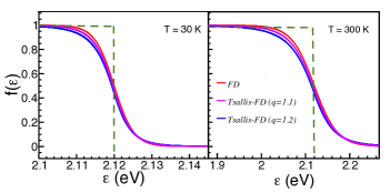
Figure 1: (Color online) Tsallis FD distribution of electrons in potassium with $\epsilon_{F}=2.12~{}eV$, for $q$=1.1 and 1.2 at two different temperatures, 30 K and 300 K. The dotted lines show the standard FD distribution for BG statistics at $T=0$ for comparison. For clarity all distributions are shown near the Fermi energy.

III Tsallis Non-Extensive Statistics and Specific Heat

In the NE thermodynamics following Tsallis formalism, one uses a $q$-deformed quantum distribution using the $q$-exponential function (given a step later). The nonextensivity enters through the parameter $q$, usually close to unity. The relevant distribution in the present case is a modified FD distribution Cleymans:2011in as given by

$$\it{f_{T}(\epsilon)}=\frac{1}{1+exp_{q}(\frac{\epsilon-\mu}{k_{B}T})},$$ (10)

where the q-exponential function, $\exp_{q}(x)$, is defined as

$$\exp_{q}(x)\equiv\left\{\begin{array}[]{l l}\left[1+(q-1)x\right]^{1/(q-1)}&~{}~{}\mathrm{if}~{}~{}~{}x>0\\ \left[1+(1-q)x\right]^{1/(1-q)}&~{}~{}\mathrm{if}~{}~{}~{}x\leq 0\\ \end{array}\right.$$ (11)

In the limit $q\rightarrow 1$, the q-exponential distribution reduces to the standard exponential form

$$\lim_{q\rightarrow 1}\exp_{q}(x)\rightarrow\exp(x).$$

Hence, the Tsallis NE distribution function in the limit of the NE parameter, $q\rightarrow 1$ goes over to the standard equilibrium FD distribution function. The parameter $q$ is a measure of the degree of non-extensivity based on the amount of correlations and possible temperature fluctuations that is not included in a pure free electron picture as described by the FD distribution. As has been mentioned earlier, in an actual case there are long range electron-ion and electron-electron correlations. The use of NE statistics will be handy for such systems, where the Tsallis form of FD distribution as given in Eq. (10) could be used.

However, as shown elsewhere,Cleymans:2012ya ; Conroy just using the $q$-deformed FD distribution function is not enough to guarantee thermodynamic consistency. In other words, the formalism must comply with standard relationships between relevant thermodynamical variables such as entropy, temperature, energy etc. This requires two additional constraints $\Sigma{{n_{i}}^{q}}=N$ and $\Sigma{{n_{i}}^{q}\epsilon_{i}}=E$ where $n_{i}$ and $\epsilon_{i}$ represent the mean occupation probability of the $i^{th}$ quantum state with energy $\epsilon_{i}$. $E$ and $N$ represent the total number of particles and the total energy respectively.

Table 1: Present list of metals, with atomic number, electron density, $\gamma$ and the estimated $q$ values. Numbers in the parentheses indicate references.

$\bf{Elements}$	$~{}z~{}~{}$	Electron-density (1028/m3)	$\epsilon_{f}$ (eV)	$\gamma_{0}~{}[\rm{mJ/(mol~{}K^{2})]}$	${\gamma_{q}}~{}[\rm{mJ/(mol~{}K^{2})]}$	$\gamma_{Exp}~{}[\rm{mJ/(mol~{}K^{2})]}$	$m^{*}/m_{0}$	$~{}q~{}$
Li	3	4.70	4.74	0.746	1.649	1.65 metals:cv	2.211	1.231
Na	11	2.65	3.24	1.091	1.381	1.38 metals:cv	1.265	1.082
Al	13	18.1	11.7	0.906	1.352	1.35 metals:cv	1.492	1.132
K	19	1.40	2.12	1.667	2.085	2.08 metals:cv	1.250	1.078
Ti	22	9.80	7.75	0.912	3.361	3.36 metals:cv	3.684	1.340
Fe	26	17.0	11.17	0.633	4.893	4.90 metals:cv	7.729	1.505
Co	27	15.63	10.58	0.668	4.410	4.40 metals:cv	6.599	1.467
Ni	28	18.2	11.74	0.602	7.032	7.04 metals:cv	11.676	1.617
Cu	29	8.47	7.0	0.505	0.690	0.69 metals:cv	1.366	1.106
Sr	38	3.55	3.95	1.790	3.645	3.64 metals:cv	2.036	1.212
Ag	47	5.86	5.49	0.644	0.648	0.64 metals:cv	1.006	1.0002
Cs	55	0.91	1.59	2.223	3.204	3.20 WLien	1.441	1.122
Au	79	5.90	5.53	0.639	0.692	0.69 metals:cv	1.083	1.028
Hg	80	8.65	7.13	0.992	1.865	1.86 metals:cv	1.880	1.193
Pb	82	13.2	9.37	1.509	2.996	2.99metals:cv	1.985	1.206

Using Tsallis NE statistics with the above mentioned constraints the total energy is given by,

$${\it U(T)}=\int_{0}^{\infty}~{}\epsilon~{}\it{f_{T}^{q}(\epsilon)}~{}\it{D}(\epsilon)d\epsilon$$ (12)

where the $q^{th}$ power of the occupation number, $f_{T}(\epsilon)$, is is used.

$$\it{f_{T}^{q}(\epsilon)}=\Bigg{(}\frac{1}{1+exp_{q}(\frac{\epsilon-\mu}{T})}\Bigg{)}^{q}.$$ (13)

So, the heat capacity is

$$\it C_{V}=\frac{\partial U}{\partial T}|_{V}=-\int_{0}^{\infty}~{}\frac{(\epsilon-\mu)^{2}}{T}~{}\frac{d\it{f_{T}^{q}(\epsilon)}}{d\epsilon}\it{D}(\epsilon)d\epsilon$$ (14)

where $D(\epsilon)$ is the density of states at $\epsilon_{F}$, given earlier in Eq. ( 9). $C_{V}$ due to electrons can now be calculated from eqn. 14 using numerical techniques as used in the present case.

In Fig. 1, we show the FD distributions as a function of energy for both BG and Tsallis statistics, respectively for the case of potassium which is a nearly perfect free electron metal with an $\epsilon_{F}$ value of $2.12~{}eV$. Results shown for the Tsallis statistics correspond to two different temperatures 30 K and 300 K. These results shown have been computed for two different $q$ values viz 1.1 and 1.2. For clarity we show only results near the Fermi energy, $\epsilon_{F}$ where differences are very clearly seen. The corresponding result for the standard FD distribution coming from BG statistics, at $T=0$, is also shown for comparison. One can clearly notice, at a given temperature, non-extensivity results in exciting more electrons to higher energy states, as compared to BG statistics based FD distribution. The net effect of this is an increased contribution to $C_{V}$. This effect becomes more and more important with increase in $q$.

IV Experimental Heat capacity in a real metal

In a real metal, at low temperature the total heat capacity can be more precisely written as

$$C_{V}=\gamma~{}T+A~{}T^{3}$$ (15)

where $\gamma$ and $A$ are constants and related to the material. Here, the first linear term is the electronic contribution in which we are interested, the second cubic term coming from lattice vibrations, based on the Debye model (phonons contribution). Therefore, at low temperatures, $C_{V}/T$ when plotted against $T^{2}$ results in a straight line. In such a case the zero intercept corresponding to $T=0$ yields the parameter $\gamma$. A compilation of this on a large number of systems is available metals:cv ; WLien .

For a free electron gas, that obeys the FD distribution, we rename the coefficient $\gamma$ as $\gamma_{0}$. This is given by

$$\gamma_{0}=\frac{\pi^{2}}{2}~{}\frac{N~{}k_{B}^{2}}{\epsilon_{F}}$$ (16)

where

$$\epsilon_{F}=\frac{\hbar^{2}}{2m}~{}k_{F}^{2}=\frac{\hbar^{2}}{2m}\Bigg{(}3~{}\pi^{2}\frac{N}{V}\Bigg{)}^{2/3}.$$ (17)

So that

$$\gamma_{0}=m\frac{\pi^{2}~{}Nk_{B}^{2}}{\hbar^{2}\Bigg{(}3~{}\pi^{2}\frac{N}{V}\Bigg{)}^{2/3}}$$ (18)

One can now see, the parameter $\gamma_{0}$ is proportional to the free electron mass. Following the same prescription as valid for free electrons obeying the FD distribution, we can now determine $\gamma$ for electrons following the Tsallis modified FD distribution as given in Eq. (10). We call it $\gamma_{q}$. This is possible provided one knows the value of the parameter $q$. In such a case the ratio $\gamma_{q}/\gamma_{0}$ can be seen as the ratio of the thermal effective mass of the electron, $m^{*}$, to free electron mass, $m$. In other words for a given system obeying the NE statistics, the parameter $q$ can be determined from a knowledge of the $m^{*}/m$ mass ratio. This is what has been followed in the present work.

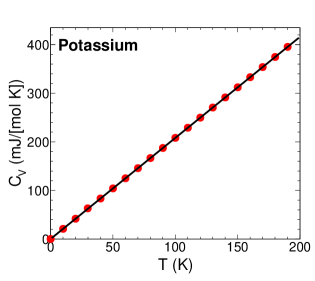
Figure 2: Electronic $C_{V}$ versus $T$ for potassium for $q$=1.078. The slope leads to a $\gamma_{q}$ value of 2.085$~{}\rm{mJ/(mol.K^{2})}$ close to the experimental data.

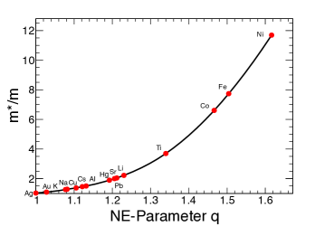
Figure 3: Ratio $m^{*}/m$ for various metals with different $q$ values. The data are well described by the the continuous line obtained using the reduced energy $\epsilon/\epsilon_{F}$ as mentioned in the text.

V Results and Discussions

In our analysis we first look at the case with potassium, a nearly perfect free electron system. In this case the total $C_{V}$ including the lattice contribution (as given by Eq. (16)) has been obtained experimentally as a function of temperature, $T$ WLien . In the low $T$ region, $C_{V}/T$ vs $T^{2}$ is shown to be perfectly linear. At $T~{}=~{}0$, $C_{V}/T=\gamma$ corresponds to the intercept which has a value of $2.08~{}\rm{mJ/(mol.K^{2})}$. Taking $\epsilon_{F}=2.12~{}eV$ as valid for potassium we estimate the parameter $q$ to have a value of 1.078 which is greater than 1. In this estimation, varying the parameter $q$, we first determine $C_{V}$ for a set of temperatures. Since there is no lattice contribution $C_{V}$ vs $T$, in accordance with Eq. (15), is perfectly linear with a zero intercept, the slope leading to $\gamma_{q}$. Our estimated $C_{V}$ data for potassium, for $q$ value of 1.078, at various temperatures is shown in Fig. 2. It has a slope ($\gamma_{q}$) value of 2.085, very close to the experimental data.

The same procedure is followed for the estimation of $q$ and $\gamma_{q}$ for other metals using the available data. As mentioned earlier, our full list includes Li, Na, Al, K, Ti, Fe, Co, Ni, Cu, Sr, Ag, Cs, Au, Hg and Pb, with 1, 2, 3 and 4 free electron systems as a complete set. The values, together with, other physical parameters such as electronic density, $\epsilon_{F}$, $\gamma_{0}$, $\gamma_{q}$ and the ratio $\gamma_{q}/\gamma_{0}$ ($=m^{*}/m$) are presented in Table 1. In the same table $m^{*}/m$ data and the experimental $\gamma_{Expt}$ values available in the literature are also included for comparison. One can see, it is possible to adjust the NE parameter $q$ to obtain $\gamma_{q}$ values close to the experimental data.

From the results included in the table, one can further see, for all metals considered in this paper, with the exception of Ag, the non-extensive parameter, $q$ deviates from unity, always being higher. This phenomenological parameter $q$ takes care of long range correlations, resulting in a higher value of $\gamma_{q}~{}(=~{}C_{V}/T)$, which in turn results in a higher value of effective mass. As has been mentioned earlier, the parameter $\gamma_{q}$ has been calculated in an earlier work Ourabah , for a number of metals, that include the present ones as well. The authors have used Tsallis modified FD statistics with a distribution function $f_{T}(\epsilon)$, different from what is used here. Their obtained $\gamma_{q}$ values for various $q$ (shown in Table 1 of ref Ourabah ) are different from what we get from the present calculations. Further, there is no agreement with experimental data metals:cv . Even the values obtained for $q~{}=1$, corresponding to pure FD distribution, are in total disagreement with free electron data, some of which are given in the present paper as $\gamma_{0}$. This is not the case with our calculations.

At the end, in Fig.3 we show a plot of the ratio $m^{*}/m$ as a function of the NE parameter $q$ as obtained in various metals considered here. The results show a nice systematic dependence, all data corresponding to different values of $\epsilon_{F}$ indicating a smooth functional dependence. The parameter $q$ distinguishes one system from another as does $\epsilon_{F}$. To check this further, for various values of $q$ in the range 1-1.7, we repeated the calculations for each of the metals considered, changing the integration variable to $\epsilon/\epsilon_{F}$ in the expression for $C_{V}$. In all the cases the scaled distribution functions fall off to zero near $\epsilon/\epsilon_{F}=1$. This actually removes the dependence on $\epsilon_{F}$ bringing out the $q$ dependence. The $\gamma_{q}$ values obtained for each system were then divided by the corresponding $\gamma_{0}$ value leading to the $m^{*}/m$ ratio as a function of $q$. Such a calculation, for each of the systems considered, results in the same smooth curve shown, passing exactly through all the points. This means, $m^{*}/m$ for all free-electron-metals, irrespective of their Fermi energies, follow a universal trend in terms of the parameter $q$.

VI Summary

In this paper, the deviation of specific heat in the free electron model from the experimentally observed value in a number of metals is explained using the Tsallis form of FD distribution function. The phenomenological NE parameter $q$, in the $q-$deformed FD distribution has been fitted to produce the experimental data. With the exception of Ag, in all cases considered, the non-extensive parameter, $q$, has been found to be greater than unity. This is mainly due to long range correlations present in the electron system. We have also obtained a nice systematic dependence of $m^{*}/m$ as a function of the NE parameter $q$, a behaviour similar to which, has not been reported.

VII Acknowledgement

GS would like to acknowledge the financial supports from the Department of Science and Technology, Govt. of India through its Women Scientist Scheme (Project No: SR/WOS-A/PM-1/2017). AK and RS acknowledge the financial supports from ALICE Project No. SR/MF/PS-01/2014-IITI(G) of Department of Science & Technology, Government of India.

References

- (1) Solid State Physics, N. W. Ashcroft and N. D. Mermin, Cengage Learning (2003).
- (2) Introduction to Nonextensive Statistical Mechanics: Approaching a Complex World, C. Tsallis, Springer Publishing (2009).
- (3) K Ourabah and M Tribeche, International Journal of Modern Physics B 27, 1350181 (2013).
- (4) A. Khuntia, S. Tripathy, R. Sahoo and J. Cleymans, Eur. Phys. J. A 53, 103 (2017)
- (5) M. D. Azmi and J. Cleymans, Eur. Phys. J. C 75, 430 (2015)
- (6) J. Cleymans, G. I. Lykasov, A. S. Parvan, A. S. Sorin, O. V. Teryaev and D. Worku, Phys. Lett. B 723, 351 (2013)
- (7) J. Cleymans and D. Worku, Eur. Phys. J. A 48, 160 (2012)
- (8) J. Cleymans and D. Worku, J. Phys. G 39, 025006 (2012)
- (9) I. Bediaga, E. M. F. Curado and J. M. de Miranda, Physica A 286, 156 (2000).
- (10) K. Urmossy, G. G. Barnafoldi and T. S. Biro, Phys. Lett. B 701, 111 (2011).
- (11) C. Tsallis, J. Statist. Phys. 52, 479 (1988).
- (12) T. Bhattacharyya, A. Khuntia, P. Sahoo, P. Garg, P. Pareek, R. Sahoo and J. Cleymans, Acta Phys. Polon. Supp. 9, 177 (2016)
- (13) T. Bhattacharyya, J. Cleymans, A. Khuntia, P. Pareek and R. Sahoo, Eur. Phys. J. A 52, 30 (2016)
- (14) A. Khuntia, P. Sahoo, P. Garg, R. Sahoo and J. Cleymans, Eur. Phys. J. A 52, 292 (2016)
- (15) G. Wilk, and Z. Wlodarczyk, Phys. Rev. Lett. 84, 2770 (2000).
- (16) T. Bhattacharyya, P. Garg, R. Sahoo and P. Samantray, Eur. Phys. J. A 52, 283 (2016)
- (17) J. M. Conroy, H. G. Miller, and A. R. Plastino, Phys. Lett A 374 4581 (2010).
- (18) http://www.knowledgedoor.com/2/elements_handbook/electronic_heat_capacity_coefficient.html
- (19) W H Lien and N E Phillips, Phy. Rev. 133, A1370 (1964).