Constraints on Lorentz Invariance and CPT Violation using Optical Photometry and Polarimetry of Active Galaxies BL Lacertae and S5 B0716+714

Abstract

Various quantum gravity approaches that extend beyond the standard model predict Lorentz Invariance and Charge-Parity-Time Violation at energies approaching the Planck scale. These models frequently predict a wavelength dependent speed of light, which would result in time delays between promptly emitted photons at different energies, as well as a wavelength-dependent rotation of the plane of linear polarization for photons resulting from vacuum birefringence. Here, we describe a pilot program with an automated system of small telescopes that can simultaneously conduct high cadence optical photometry and polarimetry of Active Galactic Nuclei (AGN) in multiple passbands. We use these observations as a proof-of-principle to demonstrate how such data can be used to test various Lorentz Violation models, including special cases of the Standard Model Extension (SME). In our initial campaign with this system, the Array Photo Polarimeter, we observed two AGN sources, including BL Lacertae at redshift $z=0.069$, and S5 B0716+714 at $z=0.31$. We demonstrate that optical polarimetry with a broadband $Luminance$ filter combined with simultaneous $I_{c}$-band observations yields SME parameter constraints that are up to $\sim$10 and $\sim$30 times more sensitive than with a standard $I_{c}$-band filter, for SME models with mass dimension $d=5$ and $d=6$, respectively. Using only a small system of telescopes with an effective $0.45$-m aperture, we further demonstrate $d=5$ constraints for individual lines of sight that are within a factor of $\sim$$1$-$10$ in sensitivity to comparable constraints from optical polarimetry with a $3.6$-m telescope. Such an approach could significantly improve existing SME constraints via a polarimetric all-sky survey of AGN with multiple 1-meter class telescopes.

I Introduction

Special relativity and the standard model of particle physics obey the symmetry of Lorentz Invariance, which has survived an enormous range of tests over the past century (See Kostelecký and Russell (2011) for a review). However, many theoretical approaches seeking to unify quantum theory and general relativity predict that Lorentz Invariance may be broken at energies approaching the Planck scale $E_{p}=\sqrt{c^{5}\hbar/G}={1.22}{\times}10^{19}{\rm\,GeV}$, perhaps due to the underlying quantized nature of spacetime (e.g. Myers and Pospelov (2003); Amelino-Camelia et al. (2015)). Since the relevant energies are not accessible to any current, or foreseeable, Earth-bound tests, most approaches to testing such models have relied on observations of high redshift astronomical sources to exploit small effects that may accumulate to detectable levels over cosmological distances and timescales.

This paper considers only Lorentz Invariance Violation (LIV) for photons, which can lead to a modified vacuum dispersion relation, and therefore an energy dependent speed of light, which causes a time delay (or early arrival) for promptly emitted photons of different energies Jacob and Piran (2008); Kostelecký and Mewes (2008). LIV models can also yield vacuum birefringence, which causes a rotation of the plane of linear polarization for promptly emitted photons at different energies emitted with the same initial polarization angle Carroll et al. (1990); Kostelecký and Mewes (2008). In general, each of these effects can be anisotropic, such that time delays and polarization rotations possess an angular dependence on the sky, and require observations of extended sources like the Cosmic Microwave Background (CMB) or measurements of point sources along many lines of sight to fully test the LIV model parameter space Kostelecký and Mewes (2009); Kislat and Krawczynski (2017).

Name	RA	DEC	Redshift $z$	$z$ Ref.	$B$	$V$	$R$	$Lum$	$I_{c}$
	IRCS(J2000)∘	IRCS(J2000)∘			(mag)	(mag)	(mag)	(mag)	(mag)
S5 0716+714	110.47270192	+71.34343428	0.31 $\pm$ 0.08	Nilsson et al. (2008); Danforth et al. (2013)	15.50	14.17	14.27	14.65	14.10
BL Lacertae	330.68038079	+42.27777231	0.0686 $\pm$ 0.0004	Vermeulen et al. (1995)	15.66	14.72	13.00	13.89	13.06

Table 1: Celestial coordinates and $BVR$ magnitudes of observed AGN sources from the Simbad database (Magnitudes may not be typical for these variable sources). $Lum$ and $I_{c}$ magnitudes are mean values from our own photometry in Tables 5-6.

Testing LIV is difficult because each of these effects are expected to be negligible at energies accessible in Earth-bound or solar system experiments. However, any such effects could, in principle, accrue to measurable levels as these tiny deviations from Lorentz symmetry accumulate over cosmological distances. Qualitatively, evidence for LIV time delays from photometric observations are easier to measure for sources at higher cosmological redshifts and higher energies Jacob and Piran (2007, 2008); Kostelecký and Mewes (2008, 2009). Compared to time delays, birefringent LIV models can be tested with much higher sensitivity using spectropolarimetry or broadband polarimetry Kostelecký and Mewes (2009).

In this work, we restrict our analysis to constraining a subset of the Standard Model Extension (SME), an effective field theory approach describing the low energy corrections stemming from a more fundamental Planck scale theory of quantum gravity. The SME therefore provides a general framework for Lorentz Invariance and Charge-Parity-Time (CPT) violation tests with electromagnetic radiation Kostelecký and Mewes (2009). More specifically, since we are only reporting observations of two optical AGN sources, we are limited to constraining either general SME models along specific lines of sight or vacuum isotropic SME models, which correspond to some of the more popular models studied in the literature. We further confine our analysis to SME models of mass operator dimension $d=4,5,6,7,8,9$. Mass dimension $d=3$ models are best constrained with observations of the CMB Kostelecký and Mewes (2008, 2009); Komatsu et al. (2009); Gubitosi et al. (2009); Kahniashvili et al. (2008); Kaufman et al. (2016a); Leon et al. (2017). While $d=4$ models can yield birefringent effects, they would not produce LIV induced time delays, since they involve no changes to the usual photon dispersion relation Kostelecký and Mewes (2009).

Simultaneous photometric observations in two filters allows one to estimate upper limits to time delays between light curves in each bandpass. While our optical time delay constraints are not competitive with observations of gamma-ray bursts Amelino-Camelia et al. (1998); Boggs et al. (2004); Ellis et al. (2006); Rodríguez Martínez and Piran (2006); Kahniashvili et al. (2006); Biesiada and Piórkowska (2007); Xiao and Ma (2009); Laurent et al. (2011); Stecker (2010, 2011); Toma et al. (2012); Kostelecký and Mewes (2013); Vasileiou et al. (2013); Pan et al. (2015); Zhang and Ma (2015); Chang et al. (2016); Lin et al. (2016); Wei et al. (2017) or TeV flares from blazars Biller et al. (1999); Albert et al. and MAGIC Collaboration (2008); Aharonian et al. and H.E.S.S. Collaboration (2008); Kostelecký and Mewes (2008); Shao et al. (2010); Tavecchio and Bonnoli (2016), our approach, which may be unique in the literature, does constrain both time delays and maximum observed polarization with simultaneously obtained photometry and polarimetry using the same pair of broadband optical filters. As such, they have the promise to compliment existing SME constraints.

Time delay measurements uniquely constrain the SME vacuum dispersion coefficients and, in principle, could constrain the vacuum birefringent coefficents as well for all models with $d\neq 4$. However, time delay measurements are typically less sensitive than broadband polarimetry for constraining the birefringent SME coefficients Kostelecký and Mewes (2009), so we exclusively use broadband polarimetry to constrain all other SME coefficients. While optical spectropolarimetry can yield constraints $\sim$$2$-$3$ orders of magnitude better for $d=5$ models than broadband optical polarimetry Kislat and Krawczynski (2017), this generally requires $\gtrsim$ 2-meter class telescopes. With telescopes less than 1-m in diameter, broadband polarimetry in two or more filters is considerably more practical, offering a solution that is low-cost and scalable to large numbers of observatories around the world. Since we did not obtain spectropolarimetry in our pilot program, we focus on the broadband polarimetry method for the rest of this work.

When observing a single source, as noted by Ellis et al. (2006), it is, in general, impossible to disentangle an intrinsic time-lag at the source from a delay induced by genuine LIV dispersion effects. Therefore, to constrain LIV models using observed time delays, one must either assume A) there are no intrinsic time delays, or B) statistically model observations of many sources using the fact that all LIV effects are predicted to increase with redshift and therefore be negligible for sufficiently “nearby” sources. For approach B, one would model the population distribution of intrinsic time lags using a calibration sample of low redshift sources and use this to disentangle these non-LIV effects from genuine LIV effects which could be manifest in a suitably matched population of higher redshift sources Ellis et al. (2006); Kostelecký and Mewes (2009); Kislat and Krawczynski (2017). However, since we only observed one nearby source (BL Lacertae at $z=0.0686\pm 0.0004$; Vermeulen et al. (1995)) and one high redshift source (S5 B0716+714 at $z=0.31\pm 0.08$, Nilsson et al. (2008); Danforth et al. (2013)), we assume option A for the remainder of this work.

Similarly, it is, in general, impossible to know the intrinsic polarization angles for photons emitted with different energies from a given cosmological source. If one possessed this information, evidence for birefringence could be obtained by observing differences between the known intrinsic polarization angle and the actual observed angles for photons emitted promptly with the same polarization angle but at different energies. However, even in the absence of such knowledge, birefringent effects can be constrained for sources at arbitrary redshifts because a large degree of birefringence would yield large differences in observed polarization angles at nearby frequencies, effectively washing out most, if not all, of the observed polarization Kostelecký and Mewes (2009, 2013); Lin et al. (2016). Therefore, observing a given polarization fraction can constrain wavelength-dependent birefringence effects, which, if in effect, would have led to a smaller degree of observed polarization. To analyze SME models in this work, we follow the “average polarization” approach in Kislat and Krawczynski (2017).

In this work, we present simultaneous photometric and polarimetric observations using two broadband optical filters on separate telescopes, including the $Luminance$-band filter ($Lum$) and a Johnson-Cousins $I$-band filter ($I_{c}$). While not as common as standard optical $BVRI$ filters, we chose the wider $Lum$ filter both to maximize the signal for our small telescopes and because wider optical bandpasses lead to tighter constraints on birefringent SME Models obtained using any of the standard optical $BVRI$ filters Kislat and Krawczynski (2017). In particular, we demonstrate significant advantages of the wider $Lum$ filter versus the narrower $I_{c}$ filter, where, for the same observed maximum polarization fraction, the $Lum$ filter yields $d=5,6$ SME parameter upper bounds that are factors of $\sim$$3$-$26$ times more sensitive than with the $I_{c}$-band filter.

In addition, we develop a technique to combine simultaneous polarimetric observations using two co-located telescopes with different filters into an effective system with a single broadband optical filter that avoids the expense of a half-wave plate with high transmission over the full $\sim$400-900 nm wavelength range of the combined $Lum+I_{c}$ filter. This yields more stringent SME constraints than either filter alone, while achieving the effective light collecting power of a larger telescope. This approach can be contrasted with an optical system using dichroic beamsplitters on a single, large telescope, to obtain simultaneous polarimetry in different bandpasses (e.g. the DIPOL-2 instrument Piirola et al. (2014)). With this approach, for the same observed maximum polarization fraction, our combined $Lum+I_{c}$ filter yields $d=5,6$ SME parameter upper bounds that are factors of $\sim$$2$-$30$ times more sensitive than with the $I_{c}$-band filter.

The pilot program in this work is meant as a proof-of-principle to obtain the most stringent SME constraints using broadband optical polarimetric observations with small telescopes for which spectropolarimetry is unfeasible. Even without spectropolarimetry, anisotropic SME constraints can be improved by observing sources along lines of sight without previously published optical polarimetry. Even if specific AGN sources already have published optical polarimetry, improved SME constraints can potentially be obtained simply by observing these sources with wider optical bandpasses, and by potentially observing a larger maximum polarization value than previously found. For all of these reasons, this work aims to motivate design feasibility studies for a follow up optical polarimetry survey using at least two 1-m class telescopes, with one or more in each hemisphere.

This paper is organized as follows. In §II, we describe the Standard Model Extension family of Lorentz and CPT-Invariance violating models we are interested in testing and present our main constraints. In §III, we describe the optical polarimetric and photometric observing systems used in this work, with emphasis on correcting for systematic errors in our maximum polarization measurements. Conclusions are presented in IV. Mathematical details, and the data obtained for this paper are presented in the Appendix.

II Standard Model Extension

We do not describe the full SME framework here. Instead, see Kostelecký and Mewes (2009) for a review. Qualitatively, if the Standard Model holds perfectly, all SME coefficients vanish identically. No strong evidence yet exists for any non-zero SME coefficients, and therefore, many LIV models falling under the SME umbrella have already been ruled out. However, the general approach to make progress testing such models is to use observations of cosmological sources at different wavelengths, higher redshifts, and varied positions on the sky to progressively lower the upper bounds for any non-zero values of the coefficients over the full SME parameter space. Weak constraints imply very large, uninformative, upper bounds. Strong constraints imply very small, informative, upper bounds that constrain coefficient values progressively closer to zero. However, even seemingly weak constraints can be of value of they are obtained with an observational approach with smaller (or different) systematics than an approach that nominally yields stronger constraints Kislat and Krawczynski (2017).

II.1 Vacuum Dispersion SME Models

Most LIV models predict a wavelength-dependent speed of light, leading to light of a given energy arriving earlier (or later) than light of another energy, even if both were emitted simultaneously in the rest frame of the source. Following Jacob and Piran (2008); Kostelecký and Mewes (2008, 2009, 2013), in the context of the SME, the arrival time difference between photons emitted simultaneously from a cosmological source with index label ${s}$ at redshift $z=z_{{s}}$ and sky position $(\theta_{{s}},\phi_{{s}})$, with observed energies $E_{1}$ and $E_{2}$, (and detected at observer frame times $t_{1}$ and $t_{2}$, respectively), is given by

$$\Delta t^{(d)}_{(z_{{s}})} = t_{2}{\scriptstyle-}t_{1}\approx\left(E_{2}^{d-4}{\scriptstyle-}E_{1}^{d-4}\right)\frac{\smash{L^{(d)}_{(z_{{s}})}}}{c}\sum_{jm}Y_{jm,{{s}}}\smash{c^{(d)}_{(I)jm}}\,,$$

where $Y_{jm,{{s}}}\equiv Y_{jm}(\theta_{{s}},\phi_{{s}})$ are the spin weighted spherical harmonics for spin-0, $\smash{c^{(d)}_{(I)jm}}$ are the vacuum dispersion SME coefficients with mass dimension $d=4,6,8,\ldots$ which must be CPT-even, and

$$\frac{\smash{L^{(d)}_{(z_{{s}})}}}{c}=\int_{0}^{z_{{s}}}\frac{(1+z)^{d-4}}{H(z)}dz=\int_{a_{{s}}}^{1}\frac{da}{(a)^{d-2}H(a)}\,,$$ (2)

where $\smash{L^{(d)}_{(z_{{s}})}}$ is the effective comoving distance traveled by the photons, including the cosmological effects needed to compute arrival time differences in an expanding universe Jacob and Piran (2008). Setting $d=4$ recovers the usual expression for comoving distance. In Eq. (2), $H(z)=H(a)$ is the Hubble expansion rate at a redshift $z_{{s}}$ with scale factor $a_{{s}}^{-1}=1+z_{{s}}$ (with the usual normalization $a(t_{0})=1$ at the present cosmic time $t=t_{0}$ at $z=0$) given by

$$H(a)=H_{0}\Big{[}\Omega_{\rm r}a^{-4}+\Omega_{\rm m}a^{-3}+\Omega_{\rm k}a^{-2}+\Omega_{\Lambda}\Big{]}^{1/2}\,,$$ (3)

in terms of the present day Hubble constant, which we set to $H_{0}=73.24$ km s^-1Mpc^-1 Riess et al. (2016), and best fit cosmological parameters for matter $\Omega_{\rm m}=0.3089$, radiation $\Omega_{\rm r}=\Omega_{\rm m}/(1+z_{eq})={9.16}{\times}10^{-5}$ (with the matter-radiation equality redshift $z_{eq}=3371$), vacuum energy $\Omega_{\Lambda}=0.6911$, and curvature $\Omega_{\rm k}=1-\Omega_{\rm r}-\Omega_{\rm m}-\Omega_{\Lambda}\approx 0$ using the Planck satellite 2015 data release Planck Collaboration et al. (2016).

In principle, observations constraining the theoretical time delay $\Delta t^{(d)}_{(z_{{s}})}$ from Eq. (LABEL:eq:deltat) between photons observed at different energies can constrain the SME coefficients $\smash{c^{(d)}_{(I)jm}}$. More specifically, an upper bound $|\Delta t_{\star}|$ on the theoretical time delay (or early arrival) $|\Delta t^{(d)}_{(z_{{s}})}|\leq|\Delta t_{\star}|$ measured from photometry in different bandpasses can be recast as an upper bound on a linear combination of SME coefficients:

$$\smash{\bar{c}^{(d)}_{(I),{{s}}}}\equiv\Big{|}\sum_{jm}Y_{jm,{{s}}}\smash{c^{(d)}_{(I)jm}}\Big{|} \lesssim \frac{c\,|\Delta t_{\star}|}{\left|E_{2}^{d-4}{\scriptstyle-}E_{1}^{d-4}\right|\smash{L^{(d)}_{(z_{{s}})}}}\,,$$ (4)

where $E_{1}$ and $E_{2}$ can be estimated from the central wavelengths of the filters. Eq. (4) defines $\smash{\bar{c}^{(d)}_{(I),{{s}}}}$ as shorthand for the absolute value of the linear combination of vacuum dispersion SME coefficients for source ${s}$.

Fig. 1 shows the relation between time delay upper limits and $d=6$ isotropic SME models for sample sources observed with both our $Lum$ and $I_{c}$ filters over a range of redshifts $z\in[0.1,1,10]$, while highlighting the parameter space already ruled out by limits from GRB observations, as well as the weaker, but meaningful constraints obtainable from optical time delay data with $|\Delta t_{\star}|\leq 1$ hour.

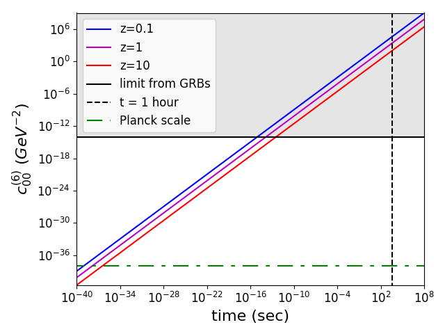
Figure 1: We plot the dimension $d=6$ isotropic vacuum dispersion SME parameter $\smash{c^{(6)}_{(I)00}}$ for time delays between two example observations in the $Lum$ and $I_{c}$ bands (central wavelengths of $\sim$550  nm vs. $\sim$800  nm) for various redshift sources ($z=0.1,1,10$). The horizontal dot-dashed line shows the $\smash{c^{(6)}_{(I)00}}$ corresponding to the Planck energy scale, while the dashed vertical line corresponds to a time delay of 1 hour. Gray regions in the parameter space with $\smash{c^{(6)}_{(I)00}}\lesssim 10^{-14}$ GeV^-2 have already been ruled out by high redshift, high time resolution, Gamma-Ray burst data Kostelecký and Mewes (2013). Because of this, optical time delays on the order of minutes to hours for moderate redshift sources can only provide weak — but still independent — constraints as a consistency check.

II.2 CPT-Odd Vacuum Birefringent SME Models

For a subset of vacuum birefringent SME models with coefficients $\smash{k^{(d)}_{(V)jm}}$, where the mass dimension $d=3,5,7,\ldots$ must be CPT-odd, rather than arrival times, the relevant quantity is the rotation of the plane of linear polarization for photons with different observed energies $E_{1}$ and $E_{2}$ that were emitted in the rest frame of the source with the same polarization angle. After traveling an effective distance of $\smash{L^{(d)}_{(z_{{s}})}}$ through an expanding universe, the difference in their observed polarization angles $\Delta\psi^{(d)}_{(z_{{s}})}=\psi_{2}{\scriptstyle-}\psi_{1}$ will be

$$\Delta\psi^{(d)}_{(z_{{s}})} \approx \left(E_{2}^{d-3}{\scriptstyle-}E_{1}^{d-3}\right)\frac{\smash{L^{(d)}_{(z_{{s}})}}}{c}\sum_{jm}Y_{jm,{{s}}}\smash{k^{(d)}_{(V)jm}}\,.$$ (5)

In principle, polarimetric observations measuring an observed polarization angle difference $|\Delta\psi_{\star}|$ in a single broadband filter with bandpass edge energies $E_{1}$ and $E_{2}$, with $|\Delta\psi^{(d)}_{(z_{{s}})}|\leq|\Delta\psi_{\star}|$, can constrain the SME coefficients $\smash{k^{(d)}_{(V)jm}}$ directly using Eq. (5),

$$\smash{\bar{k}^{(d)}_{(V),{{s}}}}\equiv\Big{|}\sum_{jm}Y_{jm,{{s}}}\smash{k^{(d)}_{(V)jm}}\Big{|} \leq \frac{c\,|\Delta\psi_{\star}|}{\Big{|}E_{2}^{d-3}{\scriptstyle-}E_{1}^{d-3}\Big{|}\smash{L^{(d)}_{(z_{{s}})}}}\,,$$ (6)

where $\smash{\bar{k}^{(d)}_{(V),{{s}}}}$ is shorthand for the absolute value of the linear combination of birefringent SME coefficients for source ${s}$.

Eq. (6) requires the assumption that all photons in the observed bandpass were emitted with the same (unknown) intrinsic polarization angle. When not making such an assumption, a more complicated and indirect argument is required. In general, when integrating over an energy range $[E_{1},E_{2}]$, if LIV effects exist, the observed polarization degree will be substantially suppressed for a given observed energy if $\Delta\psi_{\star}>\pi$, regardless of the intrinsic polarization fraction at the corresponding rest frame energy Kostelecký and Mewes (2013); Kislat and Krawczynski (2017). Other authors present arguements allowing them to assume $\Delta\psi_{\star}\leq\pi/2$ to derive bounds on certain SME models Toma et al. (2012). In our case, observing a polarization fraction $p_{\star}$ can be used to constrain birefringent SME coefficients as follows.

First, one conservatively assumes a 100% intrinsic polarization fraction at the source for all wavelengths. Lower fractions for the source polarization spectrum would lead to tighter SME bounds. In this case, the total intensity $I$ is equal to the polarized intensity $I_{p}$, such that

$$I=\int_{E_{1}}^{E_{2}}T(E)dE=I_{p}\,,$$ (7)

where $T(E)$ is the total throughput transmission function as a function of photon energy $E=hc/\lambda$ (with wavelength $\lambda$) for the polarimeter, including the relevant optics, broadband filters, and detectors (see Fig. 2). Then, following Kislat and Krawczynski (2017), integrating Eq. (5) over the energy range of the effective bandpass $T(E)$ yields normalized linear polarization Stokes parameters $q\equiv Q/I$ and $u\equiv U/I$, given by

$$\smash{q^{(d)}_{(z_{{s}})}}=\frac{I_{p}}{I}\int_{E_{1}}^{E_{2}}\cos\Big{(}2\Delta\psi\Big{)}T(E)dE$$ (8)

$$=\int_{E_{1}}^{E_{2}}\cos\Big{(}2\left(E^{d-3}{\scriptstyle-}E_{1}^{d-3}\right)\smash{L^{(d)}_{(z_{{s}})}}\smash{\bar{k}^{(d)}_{(V),{{s}}}}\Big{)}T(E)dE\,,$$

and

$$\smash{u^{(d)}_{(z_{{s}})}}=\frac{I_{p}}{I}\int_{E_{1}}^{E_{2}}\sin\Big{(}2\Delta\psi\Big{)}T(E)dE$$ (9)

$$=\int_{E_{1}}^{E_{2}}\sin\Big{(}2\left(E^{d-3}{\scriptstyle-}E_{1}^{d-3}\right)\smash{L^{(d)}_{(z_{{s}})}}\smash{\bar{k}^{(d)}_{(V),{{s}}}}\Big{)}T(E)dE\,,$$

where the intensity normalized Stokes parameters $q=\smash{q^{(d)}_{(z_{{s}})}}$ and $u=\smash{u^{(d)}_{(z_{{s}})}}$ depend on mass dimension $d$ and redshift $z_{{s}}$ in the SME framework.

An upper bound on the observed polarization is then

$$p_{\star}-2\sigma_{\star}<\smash{p_{max,(z_{{s}})}^{(d)}}=\sqrt{\Big{(}\smash{q^{(d)}_{(z_{{s}})}}\Big{)}^{2}+\Big{(}\smash{u^{(d)}_{(z_{{s}})}}\Big{)}^{2}}\,,$$ (10)

such that observing a polarization fraction $p_{\star}$ implies an upper bound on $\smash{\bar{k}^{(d)}_{(V),{{s}}}}$ by finding the largest value of $\smash{\bar{k}^{(d)}_{(V),{{s}}}}$ that is consistent with the inequality $\smash{p_{max,(z_{{s}})}^{(d)}}>p_{\star}-2\sigma_{\star}$, where $\sigma_{\star}$ is the 1-$\sigma$ uncertainty on the polarization measurement. This corresponds to a 95% confidence interval assuming Gaussian measurement errors for the polarization fraction.

As shown by Kislat and Krawczynski (2017), in this framework, broader filters lead to smaller values for $\smash{p_{max,(z_{{s}})}^{(d)}}$, so observing larger $p_{\star}$ values in those filters leads to tighter constraints on $\smash{\bar{k}^{(d)}_{(V),{{s}}}}$ than observing the same polarization $p_{\star}$ through a narrower filter for the same source. In addition to improving our signal-to-noise, this is a key reason we chose the broader $Lum$ band filter to compare to the more standard $I_{c}$ band filter, and implemented a method to combine both filters using simultaneous observations on two telescopes. The transmission $T(\lambda)$ for our combined $Lum+I_{c}$-band polarimetry is shown in Fig. 2, which can be used to compute $T(E)$. Our observational setup is described in § III.

In principle, one should also consider the source spectrum and the atmospheric attenuation in computing $T(E)$, but we follow Kislat and Krawczynski (2017) and assume that the optical spectra are flat enough in the relevant wavelength range so that we can ignore these small effects. However, unlike Kislat and Krawczynski (2017), which only consider the transmission function of the broadband filter, we additionally consider the transmission functions for the optics and CCD detector, in addition to the filter, when computing $T(E)$ (see Fig. 8).

Following Kislat and Krawczynski (2017), to jointly parametrize the cosmological redshift dependence and SME parameter effects, we define the quantity $\smash{\zeta_{{s}}^{(5)}}$ as

$$\smash{\zeta_{{s}}^{(5)}}\equiv\smash{L^{(5)}_{(z_{{s}})}}\smash{\bar{k}^{(5)}_{(V),{{s}}}}\,.$$ (11)

Also following Kislat and Krawczynski (2017), Fig. 3 shows the change in the intensity normalized Stokes parameter $\smash{q^{(d)}_{(z_{{s}})}}$ from Eq. (II.2) for several values of $\smash{\zeta_{{s}}^{(5)}}$, while Fig. 4 shows theoretical limits from the maximum observed polarization $p_{max}$ versus $\smash{\zeta_{{s}}^{(5)}}$ in our $Lum$ and $I_{c}$ bands, and for our combined $Lum+I_{c}$-band in Fig. 2. Based on Fig. 4, Fig. 5 shows that the $Lum+I_{c}$ band yields $|\smash{\zeta_{{s}}^{(5)}}|$ constraints $\sim$$2$-$10$ times more restrictive than the $I_{c}$ band for the same observed polarization fraction, over the range $p_{max}\gtrsim 0.02$, (where $p_{\star}<p_{max}$), assuming negligible uncertainties, $\sigma_{\star}$.

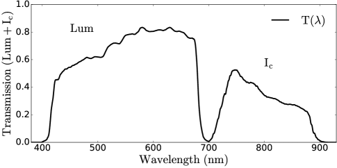
Figure 2: Total transmission function from optics, filters, and CCD detectors for our $Lum$ and $I_{c}$-bands observed using the Array Photo Polarimeter (APPOL, see §III), which we combine into a single, effective broadband $Lum+I_{c}$ filter with coverage from $\sim$400-900 nm (with minimal filter overlap at $\sim$700 nm), using simultaneous data from two telescopes (see Fig. 8).

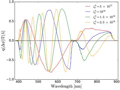
Figure 3: Change of the Stokes parameter $\smash{q^{(d)}_{(z_{{s}})}}$ from Eq. (II.2) for our combined $Lum+I_{c}$ filter in Fig. 2 for several values of $\smash{\zeta_{{s}}^{(5)}}$. For comparison, see Fig. 2 of Kislat and Krawczynski (2017).

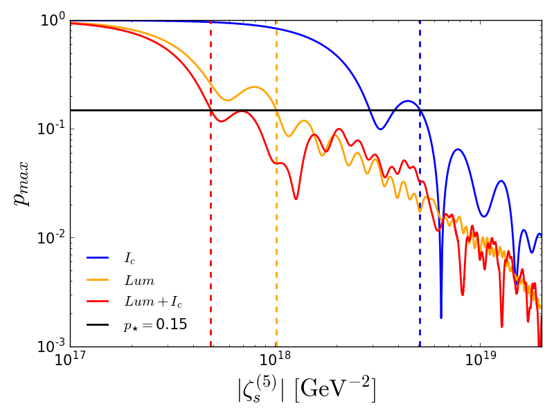
Figure 4: Maximum allowed polarization fraction $p_{max}$ vs. $d=5$ CPT-Odd Vacuum birefringence parameter $|\smash{\zeta_{{s}}^{(5)}}|$ from Eq. (11) for the $I_{c}$-band (blue), $Lum$-band (orange), and our combined $Lum+I_{c}$-band (red). For an example observed polarization fraction $p_{\star}=0.15$ (horizontal black line), upper limits on $|\smash{\zeta_{{s}}^{(5)}}|$ for each band (dashed vertical lines) can be obtained by noting that $p_{max}$ eventually falls below the observed value of $p_{\star}$ for all values of that coefficient. For $p_{\star}\gtrsim 0.02$, the most stringent upper limit comes from the combined $Lum+I_{c}$-band. For $p_{\star}=0.15$, this yields a $Lum+I_{c}$-band upper limit $|\smash{\zeta_{{s}}^{(5)}}|\lesssim 5.0\times 10^{17}$ GeV^-2, a factor of $\sim$$10$ better than the corresponding limit from the $I_{c}$ band.

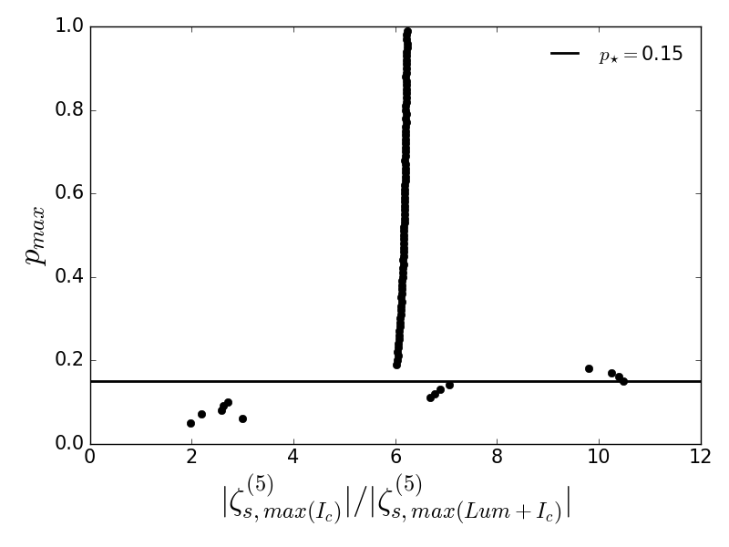
Figure 5: Theoretical maximum observed polarization $p_{max}$ vs. the ratio of CPT-odd vacuum birefringent $d=5$ SME coefficients from Fig. 4 from the $I_{c}$ and $Lum+I_{c}$ bands, $|\smash{\zeta_{{s}}^{(5)}}(I_{c})|/|\smash{\zeta_{{s}}^{(5)}}(Lum+I_{c})|$. Ignoring polarization uncertainties $\sigma_{\star}$, for all observed polarization fractions $p_{\star}\gtrsim 0.02$ (where $p_{\star}<p_{max}$), constraints from the $Lum+I_{c}$ band are $\sim$$2$-$10$ times tighter than for the $I_{c}$-band. The spike at $|\smash{\zeta_{{s}}^{(5)}}(I_{c})|/|\smash{\zeta_{{s}}^{(5)}}(Lum+I_{c})|\sim 6$ results from the fact that the ratio of the $|\smash{\zeta_{{s}}^{(5)}}|$ values in each band (blue and red curves in Fig. 4) is nearly constant for $p_{\star}\gtrsim 0.17$.

II.3 CPT-Odd Vacuum Isotropic SME Models

Since $jm$ are the angular quantum numbers with $-j\leq m\leq j$, with $j\leq d-2$, for each value of $d$, the number of distinct SME coefficients increases (See Table II of Kostelecký and Mewes (2013)). For example, the $d=5$ model has 16 SME coefficients Kislat and Krawczynski (2017). Since we only observed two sources, we are limited to constraining only linear combinations of SME coefficients $\smash{c^{(d)}_{(I)jm}}$ and $\smash{k^{(d)}_{(V)jm}}$ along two specific lines of sight. Ultimately, progressively larger numbers of sources at different locations on the sky are required to better constrain the general anisotropic model space for a given value of $d$.

However, we can follow a simpler approach and also test the subset of isotropic models, which are recovered for each value of $d$ when setting $j=m=0$. Lines of sight to individual point sources are therefore most useful for constraining the isotropic SME coefficients $\smash{c^{(d)}_{(I)00}}$ and $\smash{k^{(d)}_{(V)00}}$, which correspond to some of the simplest LIV models in the literature Kostelecký and Mewes (2009, 2013). Constraints for both isotropic SME models and linear combinations along our specific lines of sight are shown in Table 2.

II.4 CPT-Even Vacuum Birefringent SME Models

There exists an additional subset of CPT-even vacuum birefringent SME models with coefficients $\smash{k^{(d)}_{(E)jm}}$ and $\smash{k^{(d)}_{(B)jm}}$, where $d=4,6,8,\ldots$, which correspond to spin-2 helicity, rather than spin-0. Let us first define

$$\smash{\bar{k}^{(d)}_{(EB),{{s}}}} \equiv \Big{|}\sum_{jm}{}_{\pm 2}Y_{jm,{{s}}}\Big{(}\smash{k^{(d)}_{(E)jm}}+i\smash{k^{(d)}_{(B)jm}}\Big{)}\Big{|}\,,$$ (12)

as shorthand for the absolute value of the linear combination of CPT-even birefringent SME coefficients for source ${s}$. Note that there do not exist isotropic models for this subset of SME parameters so there are no $jm=00$ terms corresponding to Eq. (12). The CPT-even case is also more complex than the CPT-odd case, because the normal modes are linearly polarized and, in general, can involve no change in the polarization angle, or mixing of linearly polarized into elliptical or circularly polarized modes Kostelecký and Mewes (2013).

We now define the accumulated phase change $\Phi$ at a given energy $E$ as

$$\Phi_{{s}}=2E^{d-3}\frac{\smash{L^{(d)}_{(z_{{s}})}}}{c}\smash{\bar{k}^{(d)}_{(EB),{{s}}}}\,.$$ (13)

In the CPT-odd vacuum birefringent case, this phase change directly resulted in a polarization angle rotation because we can split linearly polarized light equally into left and right circularly polarized states. But the same is not true of the CPT-even case. Linearly polarized light will not in general be split evenly between the normal modes of a CPT-even Lorentz violation.

But similar to the CPT-odd case, we can still arrive at an expression for the maximum allowed polarization given a particular broadband filter. Again assuming a 100% polarized source at all wavelengths, the observation of a linear polarization fraction $p_{\star}$ (with uncertainty $\sigma_{\star}$) in a given broad energy band can be used to constrain the quantity $\smash{\bar{k}^{(d)}_{(EB),{{s}}}}$.

Following Kostelecký and Mewes (2013), let us first define the angle $\Psi=\psi_{0}-\psi_{b}$ as the difference between the initial polarization angle $\psi_{0}$ for light not produced in a normal mode and the initial polarization angle $\psi_{b}$ for the slower of the two normal modes. For simplicity, we omit the source index ${s}$ from the notation for $\Psi,\psi_{0}$, and $\psi_{b}$, since we will soon make assumptions which remove the $\Psi$ dependence.

Additionally we can define $\langle\cos\Phi_{{s}}\rangle$ as the average value of $\cos\Phi_{{s}}$ for source ${s}$ after integrating over the relevant energy band

$$\langle\cos\Phi_{{s}}\rangle=\int_{E_{1}}^{E_{2}}\cos\Big{(}2\left(E^{d-3}{\scriptstyle-}E_{1}^{d-3}\right)\smash{L^{(d)}_{(z_{{s}})}}\smash{\bar{k}^{(d)}_{(EB),{{s}}}}\Big{)}T(E)dE\,.$$

(14)

In this case, as shown in Appendix A, the normalized Stokes parameters $q=\smash{q^{(d)}_{(z_{{s}})}}$ and $u=\smash{u^{(d)}_{(z_{{s}})}}$ are

$$\smash{q^{(d)}_{(z_{{s}})}} = \cos 2\Psi\cos 2\psi_{b}-\langle\cos\Phi_{{s}}\rangle^{2}\sin 2\Psi\sin 2\psi_{b}\,,$$ (15)

$$\smash{u^{(d)}_{(z_{{s}})}} = \cos 2\Psi\sin 2\psi_{b}+\langle\cos\Phi_{{s}}\rangle^{2}\sin 2\Psi\cos 2\psi_{b}\,,$$ (16)

and, via Eq. (10), the corresponding maximum limit on polarization is

$$p_{\star}-2\sigma_{\star}<\smash{p_{max,(z_{{s}})}^{(d)}}\,$$

$$=\sqrt{1-\left(1-\langle\cos\Phi_{{s}}\rangle^{2}\right)\sin^{2}2\Psi}\leq|\langle\cos\Phi_{{s}}\rangle|\,,$$ (17)

where the conservative upper bound is reached when $\Psi=\pi/4$. Fig. 6 shows the corresponding limits obtained in this most conservative case.

Similar to Fig. 4, Fig. 6 shows limits from the theoretical maximum polarization $p_{max}$ in our $Lum$, $I_{c}$, and $Lum+I_{c}$-bands versus the quantity $\smash{\zeta_{{s}}^{(6)}}$, defined as

$$\smash{\zeta_{{s}}^{(6)}}\equiv\smash{L^{(6)}_{(z_{{s}})}}\smash{\bar{k}^{(6)}_{(EB),{{s}}}}\,.$$ (18)

Again, similar to Fig. 5, Fig. 7 shows that the combined $Lum+I_{c}$-band yields $|\smash{\zeta_{{s}}^{(6)}}|$ constraints up to $\sim$$3$-$30$ times more sensitive than the $I_{c}$-band.

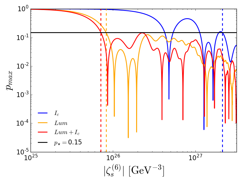
Figure 6: Similar to Fig. 4, but for $p_{max}$ vs. the $d=6$ CPT-Even Vacuum Birefringence parameter $|\smash{\zeta_{{s}}^{(6)}}|$ from Eq. (18). For an example observed polarization fraction $p_{\star}=0.15$ (horizontal black line), the most stringent upper limit of $|\smash{\zeta_{{s}}^{(6)}}|\lesssim 7\times 10^{25}$ GeV^-3 (dashed red line) comes from our combined $Lum+I_{c}$-band, a factor of $\sim$$30$ better than the corresponding limit from the $I_{c}$ band (dashed blue line).

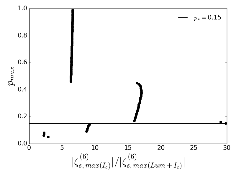
Figure 7: Similar to Fig. 5, but for $p_{max}$ vs. the ratio of CPT-even vacuum birefringent $d=6$ SME coefficients from Fig. 6 from the $I_{c}$ and $Lum+I_{c}$ bands, $|\smash{\zeta_{{s}}^{(6)}}(I_{c})|/|\smash{\zeta_{{s}}^{(6)}}(Lum+I_{c})|$. Again, ignoring polarization uncertainties $\sigma_{\star}$, for all observed polarization fractions $p_{\star}\gtrsim 0.1$ and for many values $p_{\star}<0.1$ (where $p_{\star}<p_{max}$), constraints from the $Lum+I_{c}$ band are $\sim$$3$-$30$ times tighter than for the $I_{c}$-band.

II.5 Constraints on SME Models

With simultaneous photometric time series in two filter bands, one can estimate upper limits to any time delays (or early arrivals) between the corresponding light curves under the simple assumption that the intrinsic light curve shapes are identical. We perform this analysis on our entire photometric time series (see Tables 5-6 and Figs. 9-14) using an open source implementation of the Discrete Correlation Function (DCF) in Python, which can be used to analyze variable time series with arbitrary sampling Edelson and Krolik (1988) (see, for example Robertson et al. (2015)). Constraints from time delays are presented in Table 2, using the methods of §II.1.

We consider possible estimated time delays $\Delta t_{\star}=m_{I}-m_{L}$ between observed photometric light curves in the $Lum$ and $I_{c}$ bands. Since our data points have a typical 8-10 minute cadence, we compute the best-fit DCF time delay using a series of DCF bin widths in the range $[5,20]$ minutes with step size $0.1$ minutes, while considering possible time delays or early arrivals in the range of $[-250,250]$ minutes for both sources. The mean and standard deviation of the set of best fit DCF time delays then yields $\Delta t_{\star}=$$26.5\pm 19.5$ minutes and $\Delta t_{\star}=$$-5.1\pm 3.3$ minutes for BL Lacertae and S5 B0716+714, respectively. Both are consistent with $\Delta t_{\star}=0$, and thus no time delay, to within the $2$-$\sigma$ uncertainties. Using the $2$-$\sigma$ errors, and remaining agnostic as to the sign of $\Delta t^{(d)}_{(z_{{s}})}$ leads to conservative time delay upper bounds of

$$|\Delta t_{\star}|\leq\max\{|\Delta t_{\star}-2\sigma_{\Delta t_{\star}}|,|\Delta t_{\star}+2\sigma_{\Delta t_{\star}}|\}\,,$$ (19)

which for the two sources yields $|\Delta t^{(d)}_{(z_{{s}})}|\leq|\Delta t_{\star}|=65.5$ minutes and $11.7$ minutes, for BL Lacertae and S5 B0716+714, respectively.

For a polarimetric time series measuring the polarization $p$ in either the $Lum$, $I_{c}$, or combined $Lum+I_{c}$-bands, one can use the maximum observed polarization $p_{\star}$ during the observing period to place limits on the SME parameters as in §II.2-II.4, with an additional correction for systematic errors described in Sec. III.1. While a longer survey could, in principle, yield larger values of $p_{\star}$, and thus, more stringent SME constraints, meaningful constraints can still be obtained for arbitrary values of $p_{\star}$, even though these are likely lower limits to the true maximum polarization. Constraints from maximum observed polarization measurements are presented in Table 2 for the $Lum$ and $I_{c}$-bands, and in Table 3 for the combined $Lum+I_{c}$-bands.

Even though we observed only two low redshift sources with small telescopes, our best $Lum$-band $d=5$ SME constraint from maximum polarization measurements of S5 B0716+714 at $z=0.31\pm 0.08$ in Tables 2-3, of $\smash{\bar{k}^{(5)}_{(V)}}<1\times 10^{-23}$ GeV^-1 is within an order of magnitude of all constraints for individual lines of sight from the 36 QSOs in the redshift range $z\in[0.634,2.936]$ analyzed in Table II of Kislat and Krawczynski (2017), where their SME parameter $\gamma_{\rm max}$ corresponds to our parameter $\smash{\bar{k}^{(5)}_{(V)}}$. More specifically, our best $d=5$ constraint is comparable to the least sensitive constraint $\gamma_{\rm max}<9.79\times 10^{-24}$ GeV^-1 from Table II of Kislat and Krawczynski (2017) (for FIRST J21079-0620 with $p_{\star}=1.12\pm 0.22\%$ at $z=0.644$), while our best constraint is only a factor of $\sim$$10$ less sensitive than the best constraint of $\gamma_{\rm max}<0.97\times 10^{-24}$ GeV^-1 (for PKS 1256 − 229 with $p_{\star}=22.32\pm 0.15\%$ at $z=1.365$). This is the case even though our analysis was arguably more conservative than Kislat and Krawczynski (2017), in regard to modeling our transmission functions, correcting for polarimetry systematics, and including uncertainties in the reported redshift measurements.

Note that the sources analyzed in Kislat and Krawczynski (2017) used linear polarization measurements from Sluse et al. (2005), which were observed using the 3.6-m telescope at the European Southern Observatory in La Silla, with the EFOSC2 polarimeter equipped with a $V$-band filter. As such, this work demonstrates that meaningful SME constraints for individual lines of sight — that are comparable to, or within a factor of 10 as sensitive as polarimetry constraints from a $3.6$-m telescope — can be readily obtained using a polarimetric $Lum+I_{c}$-band system of small telescopes with an effective $0.45$-m aperture, with $\sim$64 times less collecting area, which we describe in Sec. III.

Source	S5 B0716+714		BL Lacertae
$(RA,DEC)$	($110.47^{\circ}$, $71.34^{\circ}$)		($330.68^{\circ}$, $42.28^{\circ}$)
Redshift $z$	0.31 $\pm$ 0.08		0.0686 $\pm$ 0.0004
Time Delay Upper Bound	$Lum$-$I_{c}$		$Lum$-$I_{c}$
$|\Delta t_{\star}|$ [minutes]	11.7		65.5
$\smash{\bar{c}^{(6)}_{(I)}}\equiv|\sum_{jm}Y_{jm}(\theta,\phi)c_{(I)jm}^{(6)}|$	$<6\times 10^{+01}$ GeV-2		$<8\times 10^{+02}$ GeV-2
$\smash{\bar{c}^{(8)}_{(I)}}\equiv|\sum_{jm}Y_{jm}(\theta,\phi)c_{(I)jm}^{(8)}|$	$<8\times 10^{+18}$ GeV-4		$<1\times 10^{+20}$ GeV-4
$|c_{(I)00}^{(6)}|$	$<2\times 10^{+02}$ GeV-2		$<3\times 10^{+03}$ GeV-2
$|c_{(I)00}^{(8)}|$	$<3\times 10^{+19}$ GeV-4		$<4\times 10^{+20}$ GeV-4
Maximum Observed Polarization	$Lum$	$I_{c}$	$Lum$	$I_{c}$
$p_{\star}$ [%]	$10.02\pm 0.44$	$8.30\pm 0.48$	$10.33\pm 0.43$	$10.50\pm 0.30$
$p_{\rm sys,ISP}$ [%]	$0.21\pm 0.27$	$0.77\pm 0.23$	$0.92\pm 0.07$	$0.46\pm 0.07$
$p_{\rm sys,int}$ [%]	0.04	0.04	0.04	0.04
$p_{\star,cor}$ [%]	$9.77\pm 0.52$	$7.49\pm 0.53$	$9.37\pm 0.44$	$10.00\pm 0.31$
$\smash{\bar{k}^{(5)}_{(V)}}\equiv|\sum_{jm}Y_{jm}(\theta,\phi)k_{(V)jm}^{(5)}|$	$<1\times 10^{-23}$ GeV-1	$<7\times 10^{-23}$ GeV-1	$<3\times 10^{-23}$ GeV-1	$<1\times 10^{-22}$ GeV-1
$\smash{\bar{k}^{(7)}_{(V)}}\equiv|\sum_{jm}Y_{jm}(\theta,\phi)k_{(V)jm}^{(7)}|$	$<2\times 10^{-6}$ GeV-3	$<1\times 10^{-5}$ GeV-3	$<4\times 10^{-6}$ GeV-3	$<2\times 10^{-5}$ GeV-3
$\smash{\bar{k}^{(9)}_{(V)}}\equiv|\sum_{jm}Y_{jm}(\theta,\phi)k_{(V)jm}^{(9)}|$	$<3\times 10^{+11}$ GeV-5	$<4\times 10^{+12}$ GeV-5	$<8\times 10^{+11}$ GeV-5	$<6\times 10^{+12}$ GeV-5
$|k_{(V)00}^{(5)}|$	$<5\times 10^{-23}$ GeV-1	$<3\times 10^{-22}$ GeV-1	$<1\times 10^{-22}$ GeV-1	$<4\times 10^{-22}$ GeV-1
$|k_{(V)00}^{(7)}|$	$<6\times 10^{-6}$ GeV-3	$<3\times 10^{-5}$ GeV-3	$<2\times 10^{-5}$ GeV-3	$<8\times 10^{-5}$ GeV-3
$|k_{(V)00}^{(9)}|$	$<1\times 10^{+12}$ GeV-5	$<1\times 10^{+13}$ GeV-5	$<3\times 10^{+12}$ GeV-5	$<2\times 10^{+13}$ GeV-5
$\smash{\bar{k}^{(4)}_{(EB)}}\equiv|\sum_{jm}{}_{2}Y_{jm}(\theta,\phi)(k_{(E)jm}^{(4)}+ik_{(B)jm}^{(4)})|$	$\lesssim 7\times 10^{-32}$	$\lesssim 2\times 10^{-31}$	$\lesssim 2\times 10^{-31}$	$\lesssim 3\times 10^{-31}$
$\smash{\bar{k}^{(6)}_{(EB)}}\equiv|\sum_{jm}{}_{2}Y_{jm}(\theta,\phi)(k_{(E)jm}^{(6)}+ik_{(B)jm}^{(6)})|$	$\lesssim 5\times 10^{-15}$ GeV-2	$\lesssim 2\times 10^{-14}$ GeV-2	$\lesssim 1\times 10^{-14}$ GeV-2	$\lesssim 5\times 10^{-14}$ GeV-2
$\smash{\bar{k}^{(8)}_{(EB)}}\equiv|\sum_{jm}{}_{2}Y_{jm}(\theta,\phi)(k_{(E)jm}^{(8)}+ik_{(B)jm}^{(8)})|$	$\lesssim 2\times 10^{+2}$ GeV-4	$\lesssim 5\times 10^{+3}$ GeV-4	$\lesssim 4\times 10^{+2}$ GeV-4	$\lesssim 1\times 10^{+4}$ GeV-4

Table 2: Upper limits on linear combinations of SME coefficients of Lorentz and CPT violation along specific lines of sight from our $Lum$ and $I_{c}$-band observations of BL Lacertae and S5 B0716+714, with sky coordinates and redshifts from Table 1. The upper portion of the table shows the vacuum dispersion coefficients $\smash{\bar{c}^{(d)}_{(I)}}$ and corresponding isotropic coefficients $\smash{c^{(d)}_{(I)00}}$ (see Fig. 1) as inferred from estimates of an upper bound on the time delay $\Delta t_{\star}$ between the observed photometry in both the $Lum$ and $I_{c}$-bands as described in Sec. II.5. The remaining rows show separate constraints from the maximum observed polarization fraction $p_{\star}$, which we correct for systematics from interstellar polarization ($p_{\rm sys,ISP}$) and instrumental polarization and zero point bias ($p_{\rm sys,inst}$), in each band via $p_{\star,cor}=p_{\star}-p_{\rm sys,ISP}-p_{\rm sys,inst}$, with corresponding statistical errors added in quadrature. To be conservative, we derive SME parameter upper bounds using the 2-$\sigma$ errors for $\Delta t_{\star}$, $p_{\star,cor}$, and Redshift $z$. The lower rows show the vacuum birefringent coefficients $\smash{\bar{k}^{(d)}_{(V)}}$ and their corresponding isotropic coefficients $\smash{k^{(d)}_{(V)00}}$, each for the CPT-odd cases $d=5,7,9$. The last three rows show the vacuum birefringence coefficients $\smash{\bar{k}^{(d)}_{(EB)}}$ for the CPT-even cases $d=4,6,8$. In each case, constraints from our observed broadband polarimetry using the wider $Lum$-band are tighter than for the $I_{c}$-band.

Source	S5 B0716+714	BL Lacertae
$(RA,DEC)$	($110.47^{\circ}$, $71.34^{\circ}$)	($330.68^{\circ}$, $42.28^{\circ}$)
Redshift $z$	0.31 $\pm$ 0.08	0.0686 $\pm$ 0.0004
Maximum Observed Polarization	$Lum+I_{c}$	$Lum+I_{c}$
$p_{\star}$ [%]	$8.64\pm 0.30$	$10.30\pm 0.28$
$p_{\rm sys,ISP}$ [%]	$0.77\pm 0.23$	$0.92\pm 0.07$
$p_{\rm sys,inst}$ [%]	0.04	0.04
$p_{\star,cor}$ [%]	$7.83\pm 0.38$	$9.34\pm 0.29$
$\smash{\bar{k}^{(5)}_{(V)}}\equiv|\sum_{jm}Y_{jm}(\theta,\phi)k_{(V)jm}^{(5)}|$	$<2\times 10^{-23}$ GeV-1	$<5\times 10^{-23}$ GeV-1
$\smash{\bar{k}^{(7)}_{(V)}}\equiv|\sum_{jm}Y_{jm}(\theta,\phi)k_{(V)jm}^{(7)}|$	$<4\times 10^{-6}$ GeV-3	$<8\times 10^{-6}$ GeV-3
$\smash{\bar{k}^{(9)}_{(V)}}\equiv|\sum_{jm}Y_{jm}(\theta,\phi)k_{(V)jm}^{(9)}|$	$<8\times 10^{+11}$ GeV-5	$<2\times 10^{+12}$ GeV-5
$|k_{(V)00}^{(5)}|$	$<9\times 10^{-23}$ GeV-1	$<2\times 10^{-22}$ GeV-1
$|k_{(V)00}^{(7)}|$	$<1\times 10^{-5}$ GeV-3	$<3\times 10^{-5}$ GeV-3
$|k_{(V)00}^{(9)}|$	$<3\times 10^{+12}$ GeV-5	$<7\times 10^{+12}$ GeV-5
$\smash{\bar{k}^{(4)}_{(EB)}}\equiv|\sum_{jm}{}_{2}Y_{jm}(\theta,\phi)(k_{(E)jm}^{(4)}+ik_{(B)jm}^{(4)})|$	$\lesssim 8\times 10^{-32}$	$\lesssim 2\times 10^{-31}$
$\smash{\bar{k}^{(6)}_{(EB)}}\equiv|\sum_{jm}{}_{2}Y_{jm}(\theta,\phi)(k_{(E)jm}^{(6)}+ik_{(B)jm}^{(6)})|$	$\lesssim 9\times 10^{-15}$ GeV-2	$\lesssim 5\times 10^{-15}$ GeV-2
$\smash{\bar{k}^{(8)}_{(EB)}}\equiv|\sum_{jm}{}_{2}Y_{jm}(\theta,\phi)(k_{(E)jm}^{(8)}+ik_{(B)jm}^{(8)})|$	$\lesssim 2\times 10^{+2}$ GeV-4	$\lesssim 4\times 10^{+2}$ GeV-4

Table 3: Same as SME coefficient limits from maximum observed polarization from Fig. 3, but for the combined $Lum$+$I_{c}$-band (see Fig. 2).

III The Array Photo Polarimeter

The observing system used in this work, the Array Photo Polarimeter (APPOL) — maintained and operated by one of us (G. Cole) — uses dual beam inversion optical polarimetry with Savart plate analyzers rotated through an image sequence with various half-wave-plate (HWP) positions. See Tinbergen (2005); Berry et al. (2005); Berry and Gledhill (2014) for the basic procedures underlying dual beam polarimetry. This approach can be contrasted with quadruple beam analyzers with Wollaston prisms such as RoboPol (e.g. King et al. (2014); Panopoulou et al. (2015); Skalidis et al. (2018)) that can obtain all the Stokes parameters in a suitably calibrated single image.

The APPOL array employs an automated telescope, filter, and instrument control system with 5 co-located telescopes on two mounts. APPOL uses two small, Celestron 11 and 14 inch, primary telescopes (C11 and C14) for polarimetry with an effective collecting area equivalent to a larger 17.8 inch (0.45-m) telescope, with added capability to obtain simultaneous photometry or polarimetry on a third smaller telescope (Celestron 8 inch = C8), along with bright star photometry and/or guiding using a fourth and fifth 5 inch telescope. APPOL is located at StarPhysics Observatory (Reno, Nevada) at an elevation of 1585 meters.

Earlier iterations of APPOL (e.g. Cole (2010)) have been progressively equipped with new automated instrumentation and image reduction software Cole (2007, 2008, 2009), and used for spectropolarimetry studies Cole (2001, 2016), including a long observing campaign presenting polarimetry and photometry of the variable star Epsilon Aurigae Cole and Stencel (2011); Cole (2012, 2013). APPOL’s polarimeter designs also helped inform the planning and hardware implementation of the University of Denver DUSTPol instrument, an optical polarimeter with low instrumental polarization that has been used to study cool star systems, including RS CVn systems and Wolf-Rayet stars Wolfe et al. (2015).

The first row of Fig. 8 shows the inputs to the total transmission vs. wavelength $T(\lambda)$ in Fig. 2 for our $Lum$ and $I_{c}$-band polarimetry using APPOL, which can be used to compute $T(E)$ as used in § II.2-II.5. The APPOL setup used in this work and the associated polarimetry data reduction and analysis methods will be described in more detail in a companion paper Friedman et al. (in preparation).

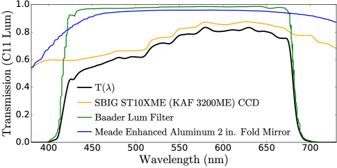
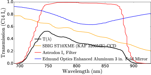
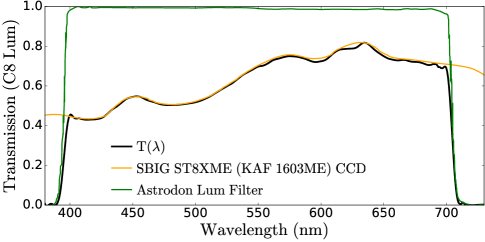
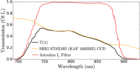
Figure 8: Array Photo Polarimeter transmission functions for the relevant optical components, filters, and CCD detectors. The first row shows the C11 and C14 telescopes used for polarimetry in the $Lum$ and $I_{c}$ bands, respectively. The second row shows the C8 telescope used for photometry in both the $I_{c}$ and $Lum$ bands. The black curve shows $T(\lambda)$, the total transmission function, which can be used to compute $T(E)$ to constrain the SME parameters via maximum polarization measurements as in § II.2-II.5. To simplify the analysis, we do not model the transmission functions of the Celestron StarBright coatings. We also do not model the transmission functions of the Savart Plates and the half-wave plates, which are fairly uniform throughout the relevant wavelength range. For similar reasons, we also neglect the atmospheric transmission or the source spectra. By comparison, the analysis in Kislat and Krawczynski (2017) only included the filter transmission function.

III.1 Observations and Systematics

All data in this paper were observed with APPOL over a short campaign in December 2017 - January 2018. Samples of the observed data for BL Lacertae (3 nights: December 14, 15, 18 (2017)) and S5 B0716+714 (5 nights: December 12, 13, 14, 15 (2017), January 1 (2018)) are shown in Appendix B in Tables 5-6, with the full machine-readable data available online and plotted in Figs. 9-11 for BL Lacertae and in Figs. 12-14 for S5 B0716+714. Image sequences with detected cosmic rays were identified as outliers and excluded. While we only use the maximum observed polarization to constrain birefringent SME models, we include the entire time series for completeness. By contrast, the full photometric time series was used to constrain the vacuum dispersion SME models using estimated time delays.

Optical photometric and polarimetric variability, correlations between flux and color, and searches for intra-band photometric time lags, have been studied extensively in the literature for AGN and BL Lacertae type objects Sluse et al. (2005); Uemura et al. (2010); Falomo et al. (2014); Hovatta et al. (2016); Kokubo (2017); Carnerero et al. (2017), including the specific, well known AGN sources we observed: BL Lacertae Moore et al. (1982); Ikejiri et al. (2011); Zhang et al. (2013, 2016), and S5 B0716+714 Impey et al. (2000); Nesci et al. (2002); Sasada et al. (2008); Larionov et al. (2013); Chandra et al. (2015); Bhatta et al. (2015, 2016); Doroshenko and Kiselev (2017); Yuan et al. (2017). Our analysis is restricted to testing SME models, but our photometric and polarimetric time series could be analyzed similarly in future work.

Our data reduction pipeline removes systematic instrumental polarization using secondary flat-field self-calibration from the two sets of images taken at the 4 half wave plate positions ($0^{\circ}$, $22.5^{\circ}$) and ($45^{\circ}$, $67.5^{\circ}$), respectively, following Berry and Gledhill (2014). Hundreds of previous APPOL measurements of unpolarized standard stars indicate that this procedure yields instrumental polarization systematics $\lesssim$ 0.03% for targets with sufficient flux, while zero-point bias adjustments are typically $\lesssim$ 0.01% for observed APPOL polarization fractions of greater than a few percent Cole (2012). The APPOL HWP waveplate modulation efficiencies have been measured to be $\gtrsim 97\%$ and $\sim 90\%$ for $Lum$ and $I_{c}$, respectively. Since imperfect modulation efficiency can only reduce the maximum observed polarization from its true value, to be conservative, we choose not to model these systematics here. Previous tests indicate that other potential systematics including coordinate frame misalignment are negligible for APPOL Cole (2012).

The total optical polarization along arbitrary lines of sight toward galactic field stars can range from a fraction of a percent to several percent Weitenbeck (2008); Meade et al. (2012); Siebenmorgen et al. (2018). Previous work from the Large Interstellar Polarization Survey provided evidence that interstellar polarization (ISP) from multiple dust clouds along a given line of sight is smaller than from lines of sight passing through a single dust cloud Bagnulo et al. and LIPS Collaboration (2017); Siebenmorgen et al. (2018). Since the presence of two or more clouds would therefore depolarize the incoming radiation, we assume that the ISP along the line of sight toward a galactic field star represents a conservative upper limit to the true ISP toward an AGN source that would have been measured through the full dust column of the galaxy, the intergalactic medium, and the AGN host galaxy.

Using a sample image sequence for each of our two AGN targets, we performed $Lum$ and $I_{c}$-band polarimetry on the two closest field stars within 3 arcmin of the target AGN, finding polarizations of $1.01\pm 0.03$% and $0.92\pm 0.07$% in $Lum$ and $0.55\pm 0.03$% and $0.46\pm 0.07$% in $I_{c}$ for the field of BL Lacertae and $0.26\pm 0.43$% and $0.21\pm 0.27$% in $Lum$ and $0.89\pm 0.73$% and $0.77\pm 0.23$% in $I_{c}$ for the field of S5 B0716+714. See Table 4. For the combined $Lum+I_{c}$ band maximum polarization measurements, we use the largest ISP systematic from the $Lum$ and $I_{c}$ bands.

Star #	GAIA DR2 ID	RA	DEC	$p_{L}$	$p_{I}$
		IRCS(J2000)∘	IRCS(J2000)∘	(%)	(%)
BL Lacertae
1	1960066324769508992	330.68924090	+42.27652024	$1.01\pm 0.03$	$0.55\pm 0.03$
2	1960066329068001536	330.69304715	+42.28231354	$0.92\pm 0.07$	$0.46\pm 0.07$
S5 B0716+714
1	1111278261916148224	110.47651216	+71.32247695	$0.26\pm 0.43$	$0.89\pm 0.73$
2	1111278158836933888	110.46803636	+71.30492029	$0.21\pm 0.27$	$0.77\pm 0.23$

Table 4: Polarization measurements $p_{L}$ ($Lum$) and $p_{I}$ ($I_{c}$) of field stars in sample image sequences within 3 arcmin of the AGN sources BL Lacertae and S5 B0716+714, used to estimate upper limits on interstellar polarization for the systematic error budget used in Tables 2-3. Celestial coordinates and GAIA DR2 identifiers from Simbad/VizieR are included.

Assuming that our AGN max polarization measurements arise from a combination of instrumental polarization, zero point bias, ISP, and intrinsic source polarization, and that the ISP is approximately constant within 3 arcmin of the AGN target line of sight, we use the smaller of the two measured stellar polarizations to estimate conservative systematic upper limits for ISP ($p_{\rm sys,ISP}$) as listed in Tables 2-3. Finally, to obtain a polarization estimate corrected for systematics, $p_{\star,cor}$, we subtract these systematic error estimates for ISP ($p_{\rm sys,ISP}$) as well as the 0.04% systematic budget from instrumental polarization and zero point bias ($p_{\rm sys,inst}$) from our maximum observed polarization in the $I_{c}$, $Lum$, and $Lum+I_{c}$-bands to obtain the SME constraints in Tables 2-3.

IV Conclusions

In this work, we performed optical polarimetry and photometry of two well known AGN sources, BL Lacertae and S5 B0716+714 in both the $Lum$ and $I_{c}$-bands, while implementing a procedure to obtain polarimetry in a wider effective passband with coverage from $\sim$$400$-$900$ nm by combining simultaneous photometry from two small, co-located telescopes. We used the ”average polarization” method of Kislat and Krawczynski (2017), which analyzed polarimetric measurements from the literature, to analyze our own polarimetric measurements, thereby demonstrating a proof-of-principle method to use our own data to derive meaningful constraints, for individual lines of sight or isotropic models, on parameters from various subsets of the Standard Model Extension, a useful framework to test for new physics beyond the Standard Model including potential violation of Lorentz and CPT Invariance Kostelecký and Mewes (2009). We demonstrated that maximum polarization measurements with our wider effective $Lum+I_{c}$ bandpass can yield SME constraints that are up to $\sim$$10$ or $\sim$$30$ times more sensitive that with our $I_{c}$-band filter, for $d=5$ and $d=6$ models, respectively.

To constrain SME parameters for a single source along a single line of sight, optical photometric measurements of AGN are not competitive with GRB gamma-ray and x-ray measurements in regard to timing resolution, energy, and redshift. Therefore, high energy GRB measurements are the best way to constrain SME parameters using observed time delays at different observed energies. Nevertheless, GRBs are transients both in their prompt gamma-ray emission and optical afterglows. Therefore, since AGN are the brightest continuous optical sources at cosmological distances, it is considerably easier to quickly obtain more complete sky coverage by observing many more AGN, in order to better constrain the anisotropic vacuum dispersion SME models. In addition, compared with gamma and x-ray polarimetry, optical polarimetric measurements typically have smaller statistical uncertainties and independent systematics Kislat and Krawczynski (2017). Optical polarimetry is also easier to obtain with ground based instruments than gamma-ray and x-ray polarimetry, which must be obtained from space (e.g. Toma et al. (2012)).

Although the limits presented here were not intended to compete with other approaches using maximum polarization measurements integrated over an optical bandpass, the pilot program in this work nevertheless demonstrates that meaningful SME constraints can be obtained even with a small set of telescopes with an effective 0.45-m aperture, that are competitive — to within a factor of $\sim$$1$-$10$ in sensitivity for $d=5$ models — even when compared to optical polarimetry from a $3.6$-m telescope Sluse et al. (2005); Kislat and Krawczynski (2017). Since $d=6$ models were not analyzed in Kislat and Krawczynski (2017), it would be interesting to perform similar comparisons to our $d=6$ constraints in future work. As such, there is a strong science case to use the maximum observed polarization for a large sample of AGN with wide optical bandpasses to constrain the anisotropic vacuum birefringent SME models, which include the three families of SME coefficients not constrained by time delay estimates.

Future work could improve upon existing SME constraints simply by using the methods in this work to analyze optical polarimetry from large published surveys of AGN and quasars (e.g Angelakis et al. (2016); Hutsemékers et al. (2017)) in addition to the AGN and GRB afterglow sources already studied by Kislat and Krawczynski (2017). In addition, state-of-the-art SME constraints could potentially be obtained by performing a new survey to significantly increase the number of high redshift sources with published optical polarimetry along independent lines of sight. The pilot program described in this work thus serves to motivate a dedicated optical AGN polarimetric survey similar to the Steward Observatory spectrapolarimetric AGN monitoring program Sluse et al. (2005), the RoboPol survey of gamma-ray selected blazars King et al. (2014); Blinov et al. (2015); Angelakis et al. (2016), or the La Silla Observatory survey of optical linear polarization of QSOs Sluse et al. (2005); Hutsemékers et al. (2017), to name some relevant examples.

Such future surveys would obtain broadband optical polarimetry of each AGN source with a set of filters, optics, and detectors optimally chosen to improve upon the SME constraints obtainable using the more standard optical filters employed by previous surveys. In addition to measuring sources along lines of sight without previously published polarimetry, where possible, polarimetric measurements of previously observed sources could still lead to tighter SME constraints by either observing a larger maximum polarization than what was reported in the literature, or by observing with a wider optical bandpass.

By duplicating this setup on one or more 1-meter class telescopes in each hemisphere, using the same data reduction software, such a survey could achieve the full sky coverage needed to fully constrain the more general anisotropic SME models at increasingly larger mass dimension $d\geq 5$. However, unlike previous surveys, it may only be necessary to observe a short duration time series for each AGN source, in order to maximize the number of sources with maximum polarization measurements, thereby optimizing a to-be-determined figure of merit which would quantify the improvement in constraints for specific SME models, during a given survey time period.

Since spectropolarimetry typically yields SME $d=5$ model parameter constraints that are $\sim$$2$-$3$ orders of magnitude more sensitive than using a single, broadband, optical filter Kislat and Krawczynski (2017), it would also be interesting to investigate the costs and benefits of a full spectropolarimetric survey on $\gtrsim 2$-m class telescopes versus a less expensive, shorter duration, survey on a set of 1-m class telescopes using multiple optical filters to test $d\geq 5$ SME models. Similarly, it would be worthwhile in future work to explore the tradeoffs for constraining SME models by using multiple, non-overlapping, narrow-band, optical filters to effectively perform low resolution spectropolarimetry versus combining two or more filters into a single, broadband filter, as demonstrated in this work.

Design feasibility studies for such a proposed survey will be analyzed in future work, with emphasis on the best path to quickly achieve the largest payoff for astrophysical tests of CPT and Lorentz Invariance violation without the time and expense required to perform an all sky spectrapolarimetric survey.

Appendix A CPT-Even Q and U

We can calculate the Stokes Q and U parameters in the presence of CPT-even SME coefficients of the form $\smash{\bar{k}^{(d)}_{(EB),{{s}}}}$ as defined in Eq. (12). As was written in Eq. (13), the phase delay between the two normal modes is given by the equation

$$\Phi(\omega)=2\omega^{d-3}L^{(d)}\smash{\bar{k}^{(d)}_{(EB),{{s}}}}\,,$$ (20)

where we denote the energy as $\omega$ as opposed to $E$ in this case to distinguish it from the electric field.

The most conservative limits on SME coefficients are obtained when we assume a broadband source emitting a uniformly linearly polarized electric field along our line of sight $\hat{z}$ in the form

$$\vec{E}(\omega,t)=Ae^{i\omega t}\hat{n}\,,$$ (21)

where $\hat{n}$ makes an angle $\phi_{0}$. Then if the slow axis of this CPT-even Lorentz violation makes an angle $\phi_{b}$ so that we can define the quantity

$$\Psi=\psi_{0}-\psi_{b}\,,$$ (22)

then the signal that reaches our detector along the slow and fast axes can be written

$$E_{slow}(\omega,t)=Ae^{i\omega t-i\Phi/2}\cos\Psi\,,$$ (23)

$$E_{fast}(\omega,t)=Ae^{i\omega t+i\Phi/2}\sin\Psi\,,$$ (24)

which, relative to our detector, is the electric field

$$\vec{E}(\omega,t) = Ae^{i\omega t}\left[e^{-i\Phi/2}\cos\Psi\cos\psi_{b}-e^{i\Phi/2}\sin\Psi\sin\phi_{b}\right]\hat{x}$$

$$+ Ae^{i\omega t}\left[e^{-i\Phi/2}\cos\Psi\sin\psi_{b}+e^{i\Phi/2}\sin\Psi\cos\phi_{b}\right]\hat{y}\,.$$

Next we can define averaging over the transmission band $T(\omega)$ as the operation

$$\left<X\right>_{\omega}=\frac{\int d\omega T(\omega)X(\omega)}{\int d\omega T(\omega)}\,,$$ (26)

so that the Stokes parameters in terms of the band averaged electric field $\vec{E}(t)=\left<\vec{E}(\omega,t)\right>_{\omega}$ incident on our detector are

$$I = |E_{x}|^{2}+|E_{y}|^{2}=|A|^{2}\,,$$ (27)

$$Q = |E_{x}|^{2}-|E_{y}|^{2}$$

$$= I\cos 2\Psi\cos 2\psi_{b}-I|\left<\cos\Phi\right>|^{2}\sin 2\Psi\sin\phi_{b}\,,$$

$$U = 2\ \mathrm{Re}(E_{x}E_{y}^{*})$$

$$= I\cos 2\Psi\sin 2\psi_{b}+I|\left<\cos\Phi\right>|^{2}\sin 2\Psi\cos\phi_{b}\,,$$

$$V = 2\ \mathrm{Im}(E_{x}E_{y}^{*})=I|\left<\sin\Phi\right>|^{2}\sin 2\Psi\,,$$ (30)

therefore the normalized Stokes parameters $q=Q/I,u=U/I$ and total linear polarization fraction $p$ are

$$q = \cos 2\Psi\cos 2\psi_{b}-|\left<\cos\Phi\right>|^{2}\sin 2\Psi\sin\phi_{b}\,,$$ (31)

$$u = \cos 2\Psi\sin 2\psi_{b}+|\left<\cos\Phi\right>|^{2}\sin 2\Psi\cos\phi_{b}\,,$$ (32)

$$p = \sqrt{\cos^{2}2\Psi+\left<\cos\Phi\right>^{2}\sin^{2}2\Psi}\,.$$ (33)

Due to the many unknowns in Eqs. (33), it is impractical to use time delays between each $q$ and $u$ time series, for example, to constrain SME vacuum birefringent parameters. Circular polarization measurements could potentially break certain degeneracies, but the maximum observed polarization approach will, in general, yield more sensitive SME constraints than any approaches using optical time delays.

Appendix B Data Plots and Tables

All data in this paper were observed with APPOL over December 2017 - January 2018. Data samples for BL Lacertae and S5 B0716+714 are shown in Tables 5-8, with the full machine-readable data to be made available online at http://cosmology.ucsd.edu and the journal website. Polarimetry is plotted in Figs. 9-11 for BL Lacertae and in Figs. 12-14 for S5 B0716+714, with photometry in Figs. 15 and 16, respectively.

MJD	$p_{L}$	$p_{I}$	$\psi_{L}$	$\psi_{I}$	$q_{L}$	$q_{I}$	$u_{L}$	$u_{I}$	$m_{L}$	$m_{I}$
(days)	(%)	(%)	(deg)	(deg)	(%)	(%)	(%)	(%)	(mag)	(mag)
58101.072	10.3 $\pm$ 0.6	9.5 $\pm$ 0.4	59.0 $\pm$ 2.0	59.0 $\pm$ 1.0	-4.9 $\pm$ 0.6	-4.4 $\pm$ 0.4	9.0 $\pm$ 0.5	8.4 $\pm$ 0.4	13.69 $\pm$ 0.03	12.93 $\pm$ 0.04
58101.079	9.0 $\pm$ 0.4	7.7 $\pm$ 0.3	63.0 $\pm$ 1.0	58.0 $\pm$ 1.0	-5.2 $\pm$ 0.4	-3.4 $\pm$ 0.3	7.3 $\pm$ 0.4	6.9 $\pm$ 0.3	13.82 $\pm$ 0.03	12.96 $\pm$ 0.04
58101.085	8.2 $\pm$ 0.4	7.9 $\pm$ 0.3	60.0 $\pm$ 1.0	59.0 $\pm$ 1.0	-4.1 $\pm$ 0.4	-3.7 $\pm$ 0.3	7.1 $\pm$ 0.4	7.0 $\pm$ 0.3	13.74 $\pm$ 0.03	12.95 $\pm$ 0.04

Table 5: Three nights of data for BL Lacertae were observed using APPOL on December 13, 14, and 17, 2017. For each Modified Julian Date (MJD), we show our observed polarimetric and photometric data for both the $Lum$ and $I_{c}$-bands, denoted by $L$ and $I$ subscripts, respectively. Columns include the observed polarization $p$ (in %), the polarization angle $\psi$ (in degrees), the intensity normalized Stokes parameters $q$ and $u$ (note that both can be negative, even when expressed as percentages), and the observed magnitude $m$. (A portion of this table is shown for guidance. This table is available in its entirety in machine-readable form.)

MJD	$p_{L}$	$p_{I}$	$\psi_{L}$	$\psi_{I}$	$q_{L}$	$q_{I}$	$u_{L}$	$u_{I}$	$m_{L}$	$m_{I}$
(days)	(%)	(%)	(deg)	(deg)	(%)	(%)	(%)	(%)	(mag)	(mag)
58099.300	8.8 $\pm$ 0.7	8.3 $\pm$ 0.5	88.0 $\pm$ 2.0	92.0 $\pm$ 2.0	-8.8 $\pm$ 0.7	-8.3 $\pm$ 0.5	0.8 $\pm$ 0.7	-0.7 $\pm$ 0.5	14.93 $\pm$ 0.04	14.39 $\pm$ 0.05
58099.306	6.9 $\pm$ 0.7	5.3 $\pm$ 0.5	81.0 $\pm$ 3.0	88.0 $\pm$ 3.0	-6.6 $\pm$ 0.7	-5.3 $\pm$ 0.5	2.1 $\pm$ 0.8	0.3 $\pm$ 0.6	15.00 $\pm$ 0.04	14.39 $\pm$ 0.05
58099.319	8.5 $\pm$ 0.7	7.6 $\pm$ 0.5	84.0 $\pm$ 2.0	88.0 $\pm$ 2.0	-8.3 $\pm$ 0.7	-7.6 $\pm$ 0.5	1.9 $\pm$ 0.7	0.6 $\pm$ 0.5	14.93 $\pm$ 0.04	14.32 $\pm$ 0.05

Table 6: Same as Table 5 but all data for S5 B0716+714, for which we observed data using APPOL over five nights on December 11-14 2017 and January 1, 2018. (A portion of this table is shown for guidance. This table is available in its entirety in machine-readable form.)

MJD	$p_{L+I}$	$\psi_{L+I}$	$q_{L+I}$	$u_{L+I}$
(days)	(%)	(deg)	(%)	(%)
58101.072	9.9 $\pm$ 0.4	59.0 $\pm$ 1.0	-4.7 $\pm$ 0.4	8.8 $\pm$ 0.4
58101.079	8.4 $\pm$ 0.3	61.0 $\pm$ 1.0	-4.5 $\pm$ 0.3	7.1 $\pm$ 0.3
58101.085	8.1 $\pm$ 0.3	59.5 $\pm$ 0.9	-3.9 $\pm$ 0.3	7.1 $\pm$ 0.3

Table 7: Same as Table 5 for BL Lacertae, but for the combined $Lum+I_{c}$-band. (A portion of this table is shown for guidance. This table is available in its entirety in machine-readable form.)

MJD	$p_{L+I}$	$\psi_{L+I}$	$q_{L+I}$	$u_{L+I}$
(days)	(%)	(deg)	(%)	(%)
58099.300	8.6 $\pm$ 0.4	89.0 $\pm$ 1.0	-8.6 $\pm$ 0.4	0.2 $\pm$ 0.4
58099.306	6.2 $\pm$ 0.5	84.0 $\pm$ 2.0	-6.1 $\pm$ 0.5	1.3 $\pm$ 0.5
58099.319	8.1 $\pm$ 0.4	85.0 $\pm$ 2.0	-8.0 $\pm$ 0.4	1.3 $\pm$ 0.4

Table 8: Same as Table 6 for S5 B0716+714, but for the combined $Lum+I_{c}$-band. (A portion of this table is shown for guidance. This table is available in its entirety in machine-readable form.)

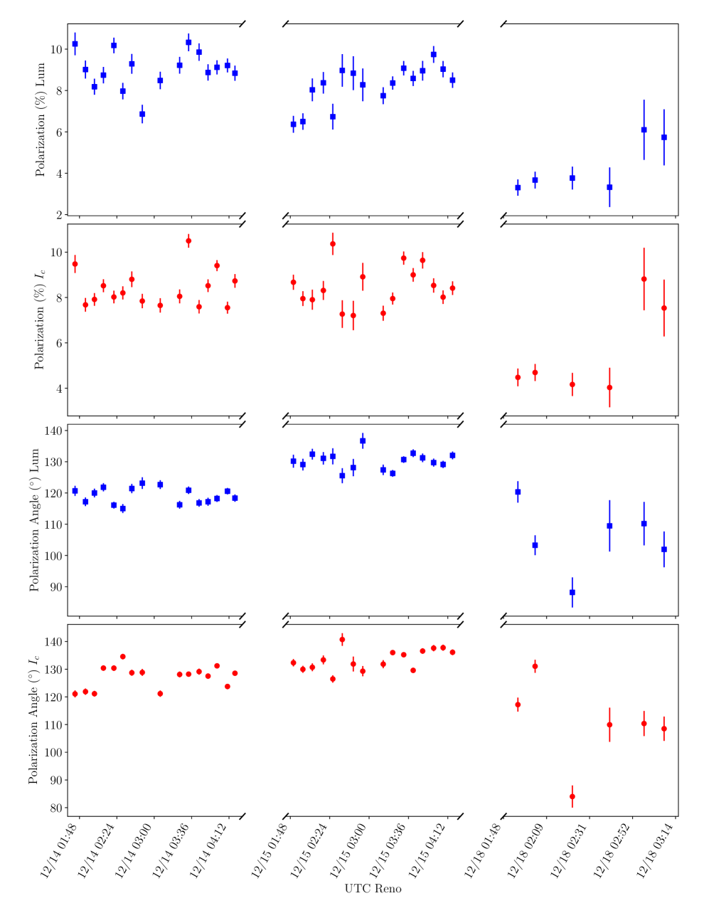
Figure 9: Polarization $p$ (in %) and polarization angle $\psi$ (in degrees) for BL Lacertae in the $Lum$ and $I_{c}$ bands.

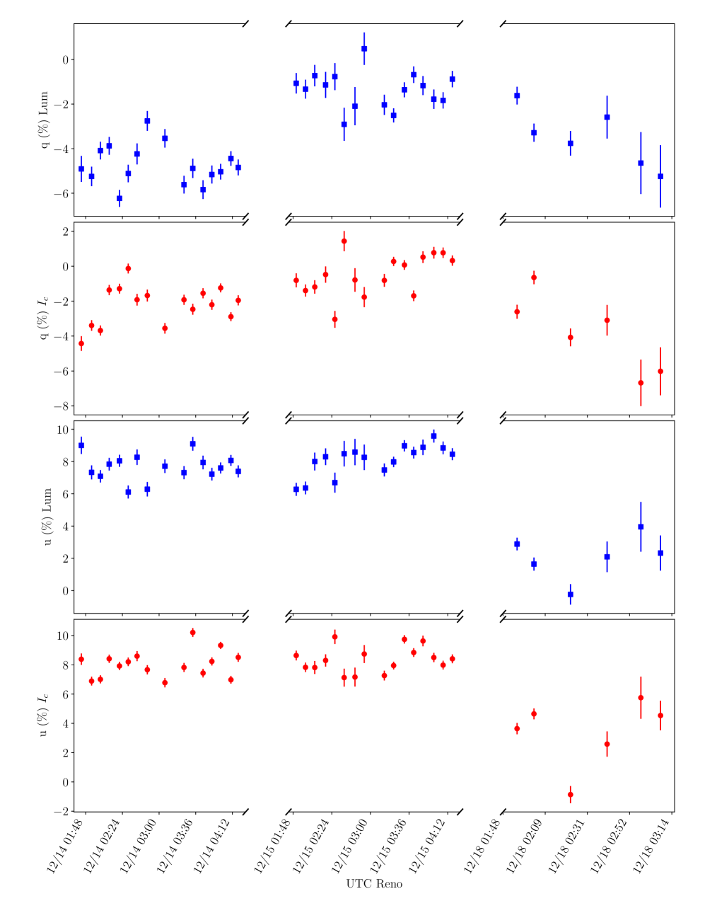
Figure 10: BL Lacertae polarimetric light curves for intensity normalized Stokes parameters $q\equiv Q/I$ and $u\equiv U/I$ in the $Lum$ and $I_{c}$ bands.

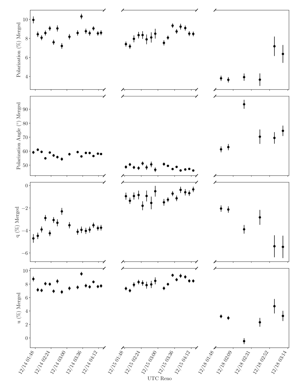
Figure 11: BL Lacertae light curves for polarization $p$ (in %), polarization angle $\psi$ (in degrees), intensity normalized Stokes parameters $q\equiv Q/I$, and $u\equiv U/I$ in the Merged $Lum+I_{c}$ band.

Figure 12: Polarization $p$ (in %) and polarization angle $\psi$ (in degrees) for S5 B0716+714 in the $Lum$ and $I_{c}$ bands.

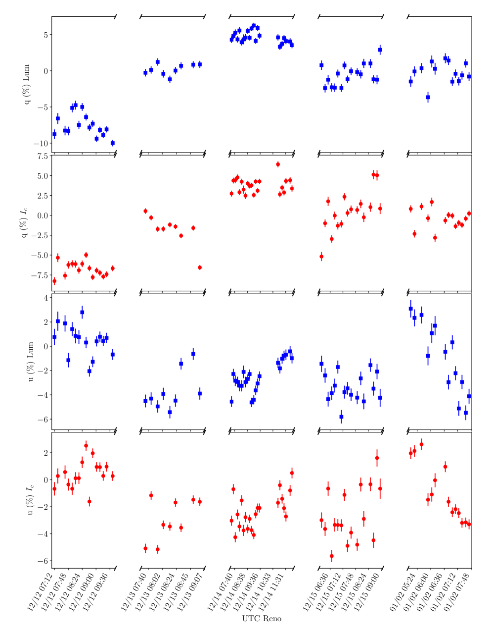
Figure 13: S5 B0716+714 polarimetric light curves for intensity normalized Stokes parameters $q\equiv Q/I$ and $u\equiv U/I$ in the $Lum$ and $I_{c}$ bands.

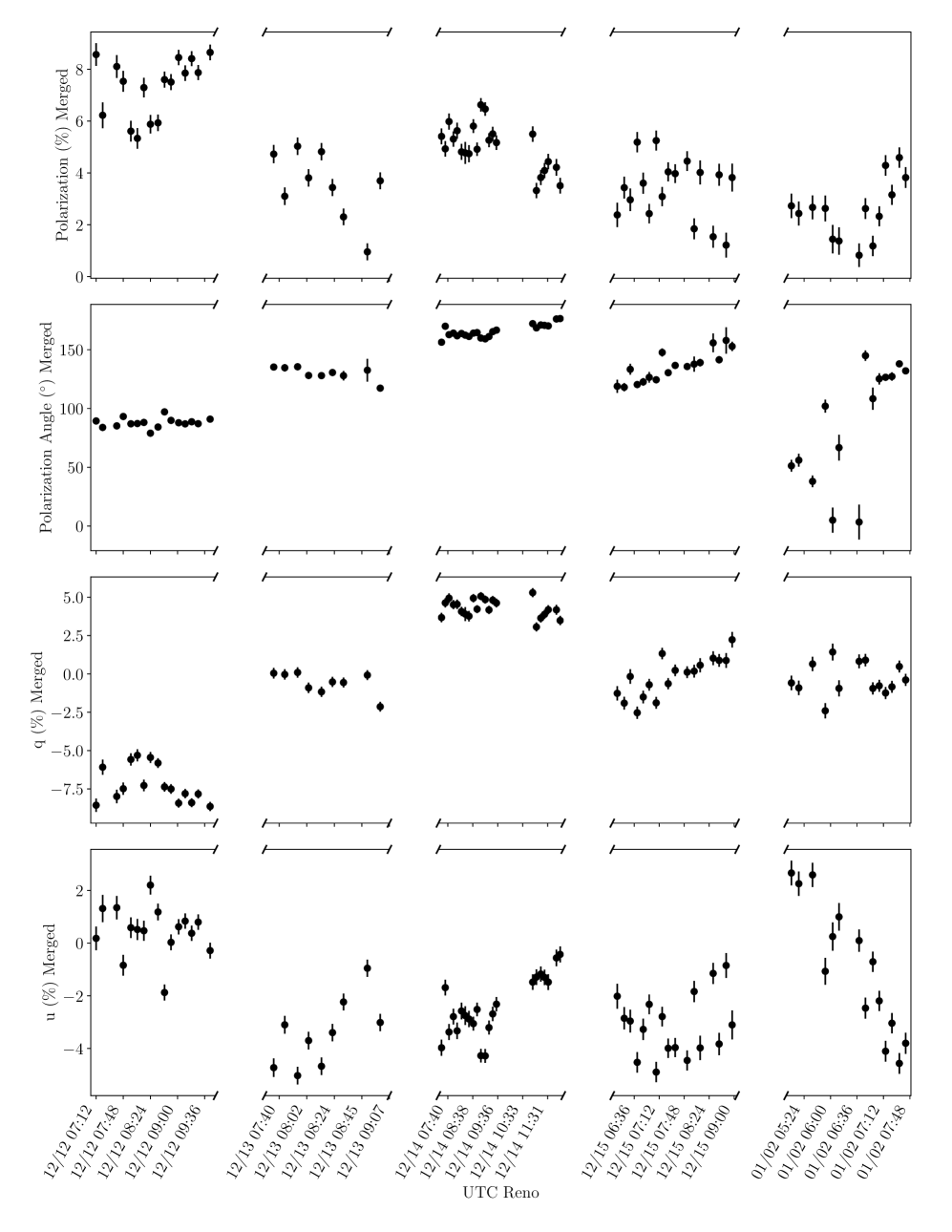
Figure 14: S5 B0716+714 light curves for polarization $p$ (in %), polarization angle $\psi$ (in degrees), intensity normalized Stokes parameters $q\equiv Q/I$, and $u\equiv U/I$ in the Merged $Lum+I_{c}$ band.

Figure 15: $I_{c}$ and $Lum$-band Photometry for BL Lacertae.

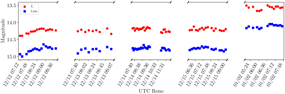
Figure 16: $I_{c}$ and $Lum$-band Photometry for S5 B0716+714.

References

- Kostelecký and Russell (2011) V. A. Kostelecký and N. Russell, “Data tables for Lorentz and CPT violation,” Rev. Mod. Phys. 83, 11–32 (2011), arXiv:0801.0287 [hep-ph] .
- Myers and Pospelov (2003) R. C. Myers and M. Pospelov, “Ultraviolet Modifications of Dispersion Relations in Effective Field Theory,” Phys. Rev. Lett. 90, 211601 (2003), hep-ph/0301124 .
- Amelino-Camelia et al. (2015) G. Amelino-Camelia, D. Guetta, and T. Piran, “ICECUBE Neutrinos and Lorentz Invariance Violation,” Astrophys. J. 806, 269 (2015).
- Jacob and Piran (2007) U. Jacob and T. Piran, “Neutrinos from gamma-ray bursts as a tool to explore quantum-gravity-induced Lorentz violation,” Nature Phys. 3, 87–90 (2007), hep-ph/0607145 .
- Jacob and Piran (2008) U. Jacob and T. Piran, “Lorentz-violation-induced arrival delays of cosmological particles,” J. Cos. Astropart. Phys. 1, 031 (2008), arXiv:0712.2170 .
- Chakraborty et al. (2013) S. Chakraborty, A. Mirizzi, and G. Sigl, “Testing Lorentz invariance with neutrino bursts from supernova neutronization,” Phys. Rev. D 87, 017302 (2013), arXiv:1211.7069 [hep-ph] .
- Stecker and Scully (2014) F. W. Stecker and S. T. Scully, “Propagation of superluminal PeV IceCube neutrinos: A high energy spectral cutoff or new constraints on Lorentz invariance violation,” Phys. Rev. D 90, 043012 (2014), arXiv:1404.7025 [astro-ph.HE] .
- Scully and Stecker (2009) S. T. Scully and F. W. Stecker, “Lorentz invariance violation and the observed spectrum of ultrahigh energy cosmic rays,” Astropart. Phys. 31, 220–225 (2009), arXiv:0811.2230 .
- Stecker (2010) F. W. Stecker, “Gamma-ray and Cosmic-ray Tests of Lorentz Invariance Violation and Quantum Gravity Models and Their Implications,” in Amer. Inst. Phys. Conf. Ser., Amer. Inst. Phys. Conf. Ser., Vol. 1223, edited by C. Cecchi, S. Ciprini, P. Lubrano, and G. Tosti (2010) pp. 192–206, arXiv:0912.0500 [hep-ph] .
- Bietenholz (2011) W. Bietenholz, “Cosmic rays and the search for a Lorentz Invariance Violation,” Phys. Rep. 505, 145–185 (2011), arXiv:0806.3713 [hep-ph] .
- Cowsik et al. (2012) R. Cowsik, T. Madziwa-Nussinov, S. Nussinov, and U. Sarkar, “Testing violations of Lorentz invariance with cosmic rays,” Phys. Rev. D 86, 045024 (2012), arXiv:1206.0713 [hep-ph] .
- Lang and de Souza (2017) R. G. Lang and V. de Souza, “Astroparticle Physics Tests of Lorentz Invariance Violation,” in Jour. Phys. Conf. Ser., Vol. 866 (2017) p. 012008, arXiv:1708.00266 [astro-ph.HE] .
- Kostelecký and Mewes (2008) V. A. Kostelecký and M. Mewes, “Astrophysical Tests of Lorentz and CPT Violation with Photons,” Astrophys. J. Lett. 689, L1 (2008), arXiv:0809.2846 .
- Carroll et al. (1990) S. M. Carroll, G. B. Field, and R. Jackiw, “Limits on a Lorentz- and parity-violating modification of electrodynamics,” Phys. Rev. D 41, 1231–1240 (1990).
- Kostelecký and Mewes (2009) V. A. Kostelecký and M. Mewes, “Electrodynamics with Lorentz-violating operators of arbitrary dimension,” Phys. Rev. D 80, 015020 (2009), arXiv:0905.0031 [hep-ph] .
- Kislat and Krawczynski (2017) F. Kislat and H. Krawczynski, “Planck-scale constraints on anisotropic Lorentz and C P T invariance violations from optical polarization measurements,” Phys. Rev. D 95, 083013 (2017), arXiv:1701.00437 [astro-ph.HE] .
- Nilsson et al. (2008) K. Nilsson, T. Pursimo, A. Sillanpää, L. O. Takalo, and E. Lindfors, “Detection of the host galaxy of S5 0716+714,” Astron. Astrophys. 487, L29–L32 (2008), arXiv:0807.0203 .
- Danforth et al. (2013) C. W. Danforth, K. Nalewajko, K. France, and B. A. Keeney, “A Fast Flare and Direct Redshift Constraint in Far-ultraviolet Spectra of the Blazar S5 0716+714,” Astrophys. J. 764, 57 (2013), arXiv:1209.3325 [astro-ph.HE] .
- Vermeulen et al. (1995) R. C. Vermeulen, P. M. Ogle, H. D. Tran, I. W. A. Browne, M. H. Cohen, A. C. S. Readhead, G. B. Taylor, and R. W. Goodrich, “When Is BL Lac Not a BL Lac?” Astrophys. J. Lett. 452, L5 (1995).
- Amelino-Camelia (2010) G. Amelino-Camelia, “Doubly-Special Relativity: Facts, Myths and Some Key Open Issues,” in Recent Developments in Theoretical Physics, edited by S. Ghosh and G. Kar (World Scientific Publishing Co, 2010) pp. 123–170, arXiv:1003.3942 .
- Smolin (2011) L. Smolin, “Classical paradoxes of locality and their possible quantum resolutions in deformed special relativity,” Gen. Rel. Grav. 43, 3671–3691 (2011), arXiv:1004.0664 [gr-qc] .
- Komatsu et al. (2009) E. Komatsu, J. Dunkley, M. R. Nolta, C. L. Bennett, B. Gold, G. Hinshaw, N. Jarosik, D. Larson, M. Limon, and L. Page et al., “Five-Year Wilkinson Microwave Anisotropy Probe Observations: Cosmological Interpretation,” Astrophys. J. Suppl. Ser. 180, 330–376 (2009), arXiv:0803.0547 .
- Gubitosi et al. (2009) G. Gubitosi, L. Pagano, G. Amelino-Camelia, A. Melchiorri, and A. Cooray, “A constraint on Planck-scale modifications to electrodynamics with CMB polarization data,” J. Cos. Astropart. Phys. 8, 021 (2009), arXiv:0904.3201 [astro-ph.CO] .
- Kahniashvili et al. (2008) T. Kahniashvili, R. Durrer, and Y. Maravin, “Testing Lorentz invariance violation with Wilkinson Microwave Anisotropy Probe five year data,” Phys. Rev. D 78, 123009 (2008), arXiv:0807.2593 .
- Kaufman et al. (2016a) J. P. Kaufman, B. G. Keating, and B. R. Johnson, “Precision tests of parity violation over cosmological distances,” Mon. Not. R. Astron Soc. 455, 1981–1988 (2016a), arXiv:1409.8242 .
- Leon et al. (2017) D. Leon, J. Kaufman, B. Keating, and M. Mewes, “The cosmic microwave background and pseudo-Nambu-Goldstone bosons: Searching for Lorentz violations in the cosmos,” Mod. Phys. Lett. A 32, 1730002 (2017), arXiv:1611.00418 .
- Kaufman et al. (2016b) J. Kaufman, D. Leon, and B. Keating, “Using the Crab Nebula as a high precision calibrator for cosmic microwave background polarimeters,” Int. Jour. Mod. Phys. D 25, 1640008 (2016b), arXiv:1602.01153 .
- Kaufman et al. (2014) J. P. Kaufman, N. J. Miller, M. Shimon, D. Barkats, C. Bischoff, I. Buder, B. G. Keating, J. M. Kovac, P. A. R. Ade, and R. Aikin et al., “Self-calibration of BICEP1 three-year data and constraints on astrophysical polarization rotation,” Phys. Rev. D 89, 062006 (2014), arXiv:1312.7877 [astro-ph.IM] .
- Amelino-Camelia et al. (1998) G. Amelino-Camelia, J. Ellis, N. E. Mavromatos, D. V. Nanopoulos, and S. Sarkar, “Tests of quantum gravity from observations of -ray bursts,” Nature (London) 393, 763–765 (1998), astro-ph/9712103 .
- Boggs et al. (2004) S. E. Boggs, C. B. Wunderer, K. Hurley, and W. Coburn, “Testing Lorentz Invariance with GRB 021206,” Astrophys. J. Lett. 611, L77–L80 (2004), astro-ph/0310307 .
- Ellis et al. (2006) J. Ellis, N. E. Mavromatos, D. V. Nanopoulos, A. S. Sakharov, and E. K. G. Sarkisyan, “Robust limits on Lorentz violation from gamma-ray bursts,” Astropart. Phys. 25, 402–411 (2006), astro-ph/0510172 .
- Rodríguez Martínez and Piran (2006) M. Rodríguez Martínez and T. Piran, “Constraining Lorentz violations with gamma ray bursts,” J. Cos. Astropart. Phys. 4, 006 (2006), astro-ph/0601219 .
- Kahniashvili et al. (2006) T. Kahniashvili, G. Gogoberidze, and B. Ratra, “Gamma ray burst constraints on ultraviolet Lorentz invariance violation,” Phys. Lett. B 643, 81–85 (2006), astro-ph/0607055 .
- Biesiada and Piórkowska (2007) M. Biesiada and A. Piórkowska, “Gamma-ray burst neutrinos, Lorenz invariance violation and the influence of background cosmology,” J. Cos. Astropart. Phys. 5, 011 (2007), arXiv:0712.0937 .
- Xiao and Ma (2009) Z. Xiao and B.-Q. Ma, “Constraints on Lorentz invariance violation from gamma-ray burst GRB090510,” Phys. Rev. D 80, 116005 (2009), arXiv:0909.4927 [hep-ph] .
- Laurent et al. (2011) P. Laurent, D. Götz, P. Binétruy, S. Covino, and A. Fernandez-Soto, “Constraints on Lorentz Invariance Violation using integral/IBIS observations of GRB041219A,” Phys. Rev. D 83, 121301 (2011), arXiv:1106.1068 [astro-ph.HE] .
- Stecker (2011) F. W. Stecker, “A new limit on Planck scale Lorentz violation from -ray burst polarization,” Astropart. Phys. 35, 95–97 (2011), arXiv:1102.2784 [astro-ph.HE] .
- Toma et al. (2012) K. Toma, S. Mukohyama, D. Yonetoku, T. Murakami, S. Gunji, T. Mihara, Y. Morihara, T. Sakashita, T. Takahashi, and Y. Wakashima et al., “Strict Limit on CPT Violation from Polarization of -Ray Bursts,” Phys. Rev. Lett. 109, 241104 (2012), arXiv:1208.5288 [astro-ph.HE] .
- Kostelecký and Mewes (2013) V. A. Kostelecký and M. Mewes, “Constraints on Relativity Violations from Gamma-Ray Bursts,” Phys. Rev. Lett. 110, 201601 (2013), arXiv:1301.5367 [astro-ph.HE] .
- Vasileiou et al. (2013) V. Vasileiou, A. Jacholkowska, F. Piron, J. Bolmont, C. Couturier, J. Granot, F. W. Stecker, J. Cohen-Tanugi, and F. Longo, “Constraints on Lorentz invariance violation from Fermi-Large Area Telescope observations of gamma-ray bursts,” Phys. Rev. D 87, 122001 (2013), arXiv:1305.3463 [astro-ph.HE] .
- Pan et al. (2015) Y. Pan, Y. Gong, S. Cao, H. Gao, and Z.-H. Zhu, “Constraints on the Lorentz Invariance Violation with Gamma-Ray Bursts via a Markov Chain Monte Carlo Approach,” Astrophys. J. 808, 78 (2015), arXiv:1505.06563 .
- Zhang and Ma (2015) S. Zhang and B.-Q. Ma, “Lorentz violation from gamma-ray bursts,” Astropart. Phys. 61, 108–112 (2015), arXiv:1406.4568 [hep-ph] .
- Chang et al. (2016) Z. Chang, X. Li, H.-N. Lin, Y. Sang, P. Wang, and S. Wang, “Constraining Lorentz invariance violation from the continuous spectra of short gamma-ray bursts,” Chin. Phys. C 40, 045102 (2016), arXiv:1506.08495 [astro-ph.HE] .
- Lin et al. (2016) H.-N. Lin, X. Li, and Z. Chang, “Gamma-ray burst polarization reduction induced by the Lorentz invariance violation,” Mon. Not. R. Astron Soc. 463, 375–381 (2016), arXiv:1609.00193 [hep-ph] .
- Wei et al. (2017) J.-J. Wei, B.-B. Zhang, L. Shao, X.-F. Wu, and P. Mészáros, “A New Test of Lorentz Invariance Violation: The Spectral Lag Transition of GRB 160625B,” Astrophys. J. Lett. 834, L13 (2017), arXiv:1612.09425 [astro-ph.HE] .
- Biller et al. (1999) S. D. Biller, A. C. Breslin, J. Buckley, M. Catanese, M. Carson, D. A. Carter-Lewis, M. F. Cawley, D. J. Fegan, J. P. Finley, and J. A. Gaidos et al., “Limits to Quantum Gravity Effects on Energy Dependence of the Speed of Light from Observations of TeV Flares in Active Galaxies,” Phys. Rev. Lett. 83, 2108–2111 (1999), gr-qc/9810044 .
- Albert et al. and MAGIC Collaboration (2008) J. Albert et al. and MAGIC Collaboration, “Probing quantum gravity using photons from a flare of the active galactic nucleus Markarian 501 observed by the MAGIC telescope,” Phys. Lett. B 668, 253–257 (2008), arXiv:0708.2889 .
- Aharonian et al. and H.E.S.S. Collaboration (2008) F. Aharonian et al. and H.E.S.S. Collaboration, “Limits on an Energy Dependence of the Speed of Light from a Flare of the Active Galaxy PKS 2155-304,” Phys. Rev. Lett. 101, 170402 (2008), arXiv:0810.3475 .
- Shao et al. (2010) L. Shao, Z. Xiao, and B.-Q. Ma, “Lorentz violation from cosmological objects with very high energy photon emissions,” Astropart. Phys. 33, 312–315 (2010), arXiv:0911.2276 [hep-ph] .
- Tavecchio and Bonnoli (2016) F. Tavecchio and G. Bonnoli, “On the detectability of Lorentz invariance violation through anomalies in the multi-TeV -ray spectra of blazars,” Astron. Astrophys. 585, A25 (2016), arXiv:1510.00980 [astro-ph.HE] .
- Biesiada and Piórkowska (2009) M. Biesiada and A. Piórkowska, “Gravitational lensing time delays as a tool for testing Lorentz-invariance violation,” Mon. Not. R. Astron Soc. 396, 946–950 (2009), arXiv:0712.0941 .
- Shao (2014) L. Shao, “Tests of Local Lorentz Invariance Violation of Gravity in the Standard Model Extension with Pulsars,” Phys. Rev. Lett. 112, 111103 (2014), arXiv:1402.6452 [gr-qc] .
- Schmidt et al. (1992) G. D. Schmidt, H. S. Stockman, and P. S. Smith, “Discovery of a sub-megagauss magnetic white dwarf through spectropolarimetry,” Astrophys. J. Lett. 398, L57–L60 (1992).
- Sluse et al. (2005) D. Sluse, D. Hutsemékers, H. Lamy, R. Cabanac, and H. Quintana, “New optical polarization measurements of quasi-stellar objects. The data,” Astron. Astrophys. 433, 757–764 (2005), astro-ph/0507023 .
- Smith et al. (2009) P. S. Smith, E. Montiel, S. Rightley, J. Turner, G. D. Schmidt, and B. T. Jannuzi, “Coordinated Fermi/Optical Monitoring of Blazars and the Great 2009 September Gamma-ray Flare of 3C 454.3,” ArXiv e-prints (2009), arXiv:0912.3621 [astro-ph.HE] .
- Piirola et al. (2014) V. Piirola, A. Berdyugin, and S. Berdyugina, “DIPOL-2: a double image high precision polarimeter,” in Ground-based and Airborne Instrumentation for Astronomy V, Proc. SPIE, Vol. 9147 (2014) p. 91478I.
- Riess et al. (2016) A. G. Riess, L. M. Macri, S. L. Hoffmann, D. Scolnic, S. Casertano, A. V. Filippenko, B. E. Tucker, M. J. Reid, D. O. Jones, and J. M. Silverman et al., “A 2.4% Determination of the Local Value of the Hubble Constant,” Astrophys. J. 826, 56 (2016), arXiv:1604.01424 .
- Planck Collaboration et al. (2016) Planck Collaboration, P. A. R. Ade, N. Aghanim, M. Arnaud, M. Ashdown, J. Aumont, C. Baccigalupi, A. J. Banday, R. B. Barreiro, and J. G. Bartlett et al., “Planck 2015 results. XIII. Cosmological parameters,” Astron. Astrophys. 594, A13 (2016), arXiv:1502.01589 .
- Edelson and Krolik (1988) R. A. Edelson and J. H. Krolik, “The discrete correlation function - A new method for analyzing unevenly sampled variability data,” Astrophys. J. 333, 646–659 (1988).
- Robertson et al. (2015) D. R. S. Robertson, L. C. Gallo, A. Zoghbi, and A. C. Fabian, “Searching for correlations in simultaneous X-ray and UV emission in the narrow-line Seyfert 1 galaxy 1H 0707-495,” Mon. Not. R. Astron Soc. 453, 3455–3460 (2015), arXiv:1507.05201 [astro-ph.HE] .
- Tinbergen (2005) J. Tinbergen, Astronomical Polarimetry (Cambridge University Press, Cambridge, UK, 2005).
- Berry et al. (2005) D. S. Berry, T. M. Gledhill, J. S. Greaves, and T. Jenness, “POLPACK—An Imaging Polarimetry Reduction Package,” in Astronomical Polarimetry: Current Status and Future Directions, Astron. Soc. Pac. Conf. Ser., Vol. 343, edited by A. Adamson, C. Aspin, C. Davis, and T. Fujiyoshi (2005) p. 71.
- Berry and Gledhill (2014) D. S. Berry and T. M. Gledhill, “POLPACK: Imaging polarimetry reduction package,” Astrophys. Source Code Lib. (2014), ascl:1405.014 .
- King et al. (2014) O. G. King, D. Blinov, A. N. Ramaprakash, I. Myserlis, E. Angelakis, M. Baloković, R. Feiler, L. Fuhrmann, T. Hovatta, and P. Khodade et al., “The RoboPol pipeline and control system,” Mon. Not. R. Astron Soc. 442, 1706–1717 (2014), arXiv:1310.7555 [astro-ph.IM] .
- Panopoulou et al. (2015) G. Panopoulou, K. Tassis, D. Blinov, V. Pavlidou, O. G. King, E. Paleologou, A. Ramaprakash, E. Angelakis, M. Baloković, and H. K. Das et al., “Optical polarization map of the Polaris Flare with RoboPol,” Mon. Not. R. Astron Soc. 452, 715–726 (2015), arXiv:1503.03054 [astro-ph.SR] .
- Skalidis et al. (2018) R. Skalidis, G. V. Panopoulou, K. Tassis, V. Pavlidou, D. Blinov, I. Komis, and I. Liodakis, “Local measurements of the mean interstellar polarization at high Galactic latitudes,” Astron. Astrophys. 616, A52 (2018), arXiv:1802.04305 .
- Cole (2010) G. M. Cole, “Developing a Polarimeter to Support the Epsilon Aurigae Campaign,” Soc. Astron. Sci. Ann. Symp. 29, 37–42 (2010).
- Cole (2007) G. M. Cole, “A Pellicle Autoguider for the DSS-7 Spectrograph,” Soc. Astron. Sci. Ann. Symp. 26, 153 (2007).
- Cole (2008) G. M. Cole, “Automating a Telescope for Spectroscopy,” Soc. Astron. Sci. Ann. Symp. 27, 103 (2008).
- Cole (2009) G. M. Cole, “A New Instrument Selector for Small Telescopes,” in Am. Astron. Soc. Meet. Abs., Vol. 214 (2009) p. 672.
- Cole (2001) G. Cole, “A Spectropolarimeter Based On The SBIG Spectrometer,” International Amateur-Professional Photoelectric Photometry Communications 84, 13 (2001).
- Cole (2016) G. M. Cole, “Small Telescope Spectropolarimetry: Instruments and Observations,” Soc. Astron. Sci. Ann. Symp. 35, 37–47 (2016).
- Cole and Stencel (2011) G. M. Cole and R. E. Stencel, “Polarimetry of Epsilon Aurigae from Mid Eclipse to Third Contact,” Soc. Astron. Sci. Ann. Symp. 30, 103–108 (2011).
- Cole (2012) G. M. Cole, “Polarimetry of epsilon Aurigae, From November 2009 to January 2012,” Jour. Am. Assoc. Var. Star Obs. 40, 787 (2012).
- Cole (2013) G. M. Cole, “Long Term Broadband Polarimetry of Epsilon Aurigae and Field Stars,” in Giants of Eclipse, Vol. 45 (2013).
- Wolfe et al. (2015) T. M. Wolfe, R. Stencel, and G. Cole, “Commissioning Results of a New Polarimeter: Denver University Small Telescope Polarimeter (DUSTPol),” in Polarimetry, IAU Symposium, Vol. 305, edited by K. N. Nagendra, S. Bagnulo, R. Centeno, and M. Jesús Martínez González (2015) pp. 200–206.
- Friedman et al. (in preparation) A. S. Friedman et al., “The Array Photo Polarimeter,” (in preparation).
- Uemura et al. (2010) M. Uemura, K. S. Kawabata, M. Sasada, Y. Ikejiri, K. Sakimoto, R. Itoh, M. Yamanaka, T. Ohsugi, S. Sato, and M. Kino, “Bayesian approach to find a long-term trend in erratic polarization variations observed in blazars,” in 38th COSPAR Scientific Assembly, COSPAR Meeting, Vol. 38 (2010) p. 2, arXiv:0911.2950 [astro-ph.CO] .
- Falomo et al. (2014) R. Falomo, E. Pian, and A. Treves, “An optical view of BL Lacertae objects,” Astron. Astrophys. Rev. 22, 73 (2014), arXiv:1407.7615 [astro-ph.HE] .
- Hovatta et al. (2016) T. Hovatta, E. Lindfors, D. Blinov, V. Pavlidou, K. Nilsson, S. Kiehlmann, E. Angelakis, V. Fallah Ramazani, I. Liodakis, and I. Myserlis et al., “Optical polarization of high-energy BL Lacertae objects,” Astron. Astrophys. 596, A78 (2016), arXiv:1608.08440 [astro-ph.HE] .
- Kokubo (2017) M. Kokubo, “Constraints on the optical polarization source in the luminous non-blazar quasar 3C 323.1 (PG 1545+210) from the photometric and polarimetric variability,” Mon. Not. R. Astron Soc. 467, 3723–3736 (2017), arXiv:1701.03798 .
- Carnerero et al. (2017) M. I. Carnerero, C. M. Raiteri, M. Villata, J. A. Acosta-Pulido, V. M. Larionov, P. S. Smith, F. D’Ammando, I. Agudo, M. J. Arévalo, and R. Bachev et al., “Dissecting the long-term emission behaviour of the BL Lac object Mrk 421,” Mon. Not. R. Astron Soc. 472, 3789–3804 (2017), arXiv:1709.02237 [astro-ph.HE] .
- Moore et al. (1982) R. L. Moore, J. R. P. Angel, R. Duerr, M. J. Lebofsky, W. Z. Wisniewski, G. H. Rieke, D. J. Axon, J. Bailey, J. M. Hough, and J. T. McGraw, “The noise of BL Lacertae,” Astrophys. J. 260, 415–436 (1982).
- Ikejiri et al. (2011) Y. Ikejiri, M. Uemura, M. Sasada, R. Ito, M. Yamanaka, K. Sakimoto, A. Arai, Y. Fukazawa, T. Ohsugi, and K. S. Kawabata et al., “Photopolarimetric Monitoring of Blazars in the Optical and Near-Infrared Bands with the Kanata Telescope. I. Correlations between Flux, Color, and Polarization,” Publ. Astron. Soc. Jap. 63, 639–675 (2011), arXiv:1105.0255 [astro-ph.HE] .
- Zhang et al. (2013) Y.-H. Zhang, F.-Y. Bian, J.-Z. Li, and R.-C. Shang, “Optical observations of BL Lacertae in 2004-2005,” Mon. Not. R. Astron Soc. 432, 1189–1195 (2013).
- Zhang et al. (2016) Y. H. Zhang, L. Xu, and J. C. Li, “Search for hard lags with intra-night optical observations of BL Lacertae,” Astronomische Nachrichten 337, 286 (2016).
- Impey et al. (2000) C. D. Impey, V. Bychkov, S. Tapia, Y. Gnedin, and S. Pustilnik, “Rapid Polarization Variability in the BL Lacertae Object S5 0716+714,” Astron. J. 119, 1542–1561 (2000).
- Nesci et al. (2002) R. Nesci, E. Massaro, and F. Montagni, “Intraday Optical Variability of S5 0716+714,” Publ. Astron. Soc. Aus. 19, 143–146 (2002).
- Sasada et al. (2008) M. Sasada, M. Uemura, A. Arai, Y. Fukazawa, K. S. Kawabata, T. Ohsugi, T. Yamashita, M. Isogai, S. Sato, and M. Kino, “Detection of Polarimetric Variations Associated with the Shortest Time-Scale Variability in S5 0716+714,” Publ. Astron. Soc. Jap. 60, L37–L41 (2008), arXiv:0812.1416 .
- Larionov et al. (2013) V. M. Larionov, S. G. Jorstad, A. P. Marscher, D. A. Morozova, D. A. Blinov, V. A. Hagen-Thorn, T. S. Konstantinova, E. N. Kopatskaya, L. V. Larionova, and E. G. Larionova et al., “The Outburst of the Blazar S5 0716+71 in 2011 October: Shock in a Helical Jet,” Astrophys. J. 768, 40 (2013), arXiv:1303.2218 [astro-ph.HE] .
- Chandra et al. (2015) S. Chandra, H. Zhang, P. Kushwaha, K. P. Singh, M. Bottcher, N. Kaur, and K. S. Baliyan, “Multi-wavelength Study of Flaring Activity in BL Lac Object S5 0716+714 during the 2015 Outburst,” Astrophys. J. 809, 130 (2015), arXiv:1507.06473 [astro-ph.HE] .
- Bhatta et al. (2015) G. Bhatta, A. Goyal, M. Ostrowski, Ł. Stawarz, H. Akitaya, A. A. Arkharov, R. Bachev, E. Benítez, G. A. Borman, and D. Carosati et al., “Discovery of a Highly Polarized Optical Microflare in Blazar S5 0716+714 during the 2014 WEBT Campaign,” Astrophys. J. Lett. 809, L27 (2015), arXiv:1507.08424 [astro-ph.HE] .
- Bhatta et al. (2016) G. Bhatta, Ł. Stawarz, M. Ostrowski, A. Markowitz, H. Akitaya, A. A. Arkharov, R. Bachev, E. Benítez, G. A. Borman, and D. Carosati et al., “Multifrequency Photo-polarimetric WEBT Observation Campaign on the Blazar S5 0716+714: Source Microvariability and Search for Characteristic Timescales,” Astrophys. J. 831, 92 (2016), arXiv:1608.03531 [astro-ph.HE] .
- Doroshenko and Kiselev (2017) V. T. Doroshenko and N. N. Kiselev, “Polarization and brightness of the blazar S5 0716+714 in 1991-2004,” Astron. Lett. 43, 365–387 (2017).
- Yuan et al. (2017) Y.-H. Yuan, J.-h. Fan, J. Tao, B.-C. Qian, D. Costantin, H.-B. Xiao, Z.-Y. Pei, and C. Lin, “Optical monitoring of BL Lac object S5 0716+714 and FSRQ 3C 273 from 2000 to 2014,” Astron. Astrophys. 605, A43 (2017), arXiv:1706.00974 .
- Hough (2005) J. H. Hough, “Polarimetry Techniques at Optical and Infrared Wavelengths,” in Astronomical Polarimetry: Current Status and Future Directions, Astron. Soc. Pac. Conf. Ser., Vol. 343, edited by A. Adamson, C. Aspin, C. Davis, and T. Fujiyoshi (2005) p. 3.
- Hough (2006) J. Hough, “Polarimetry: a powerful diagnostic tool in astronomy,” Astron. Geophys. 47, 3.31–3.35 (2006).
- Hough (2007) J. H. Hough, “New opportunities for astronomical polarimetry,” Jour. Quant. Spec. Rad. Trans. 106, 122–132 (2007).
- Hough (2011) J Hough, “High sensitivity polarimetry: techniques and applications,” Polarimetric Detection, Characterization and Remote Sensing , 177–204 (2011).
- Bagnulo et al. (2009) S. Bagnulo, M. Landolfi, J. D. Landstreet, E. Landi Degl’Innocenti, L. Fossati, and M. Sterzik, “Stellar Spectropolarimetry with Retarder Waveplate and Beam Splitter Devices,” Publ. Astron. Soc. Pac. 121, 993 (2009).
- Canovas et al. (2011) H. Canovas, M. Rodenhuis, S. V. Jeffers, M. Min, and C. U. Keller, “Data-reduction techniques for high-contrast imaging polarimetry. Applications to ExPo,” Astron. Astrophys. 531, A102 (2011), arXiv:1105.2961 [astro-ph.IM] .
- Weitenbeck (2008) A. J. Weitenbeck, “Stars with ISM Polarization Observed with HPOL. III,” Acta Astronomica 58, 433 (2008).
- Meade et al. (2012) M. R. Meade, B. A. Whitney, B. L. Babler, K. H. Nordsieck, K. S. Bjorkman, and J. P. Wisniewski, “HPOL: World’s largest database of optical spectropolarimetry,” in Amer. Inst. Phys. Conf. Ser., Amer. Inst. Phys. Conf. Ser., Vol. 1429, edited by J. L. Hoffman, J. Bjorkman, and B. Whitney (2012) pp. 226–229.
- Siebenmorgen et al. (2018) R. Siebenmorgen, N. V. Voshchinnikov, S. Bagnulo, N. L. J. Cox, J. Cami, and C. Peest, “Large Interstellar Polarisation Survey. II. UV/optical study of cloud-to-cloud variations of dust in the diffuse ISM,” Astron. Astrophys. 611, A5 (2018), arXiv:1711.08672 .
- Bagnulo et al. and LIPS Collaboration (2017) Bagnulo et al. and LIPS Collaboration, “Large Interstellar Polarisation Survey (LIPS). I. FORS2 spectropolarimetry in the Southern Hemisphere,” Astron. Astrophys. 608, A146 (2017), arXiv:1710.02439 [astro-ph.SR] .
- Angelakis et al. (2016) E. Angelakis, T. Hovatta, D. Blinov, V. Pavlidou, S. Kiehlmann, I. Myserlis, M. Böttcher, P. Mao, G. V. Panopoulou, and I. Liodakis et. al, “RoboPol: the optical polarization of gamma-ray-loud and gamma-ray-quiet blazars,” Mon. Not. R. Astron Soc. 463, 3365–3380 (2016), arXiv:1609.00640 [astro-ph.HE] .
- Hutsemékers et al. (2017) D. Hutsemékers, P. Hall, and D. Sluse, “Optical linear polarization measurements of quasars obtained with the 3.6 m telescope at the La Silla Observatory,” Astron. Astrophys. 606, A101 (2017), arXiv:1709.01309 .
- Blinov et al. (2015) D. Blinov, V. Pavlidou, I. Papadakis, S. Kiehlmann, G. Panopoulou, I. Liodakis, O. G. King, E. Angelakis, M. Baloković, and H. Das et al., “RoboPol: first season rotations of optical polarization plane in blazars,” Mon. Not. R. Astron Soc. 453, 1669–1683 (2015), arXiv:1505.07467 [astro-ph.HE] .