Bayesian Double Feature Allocation for Phenotyping with Electronic Health Records

Abstract

We propose a categorical matrix factorization method to infer latent diseases from electronic health records (EHR) data in an unsupervised manner. A latent disease is defined as an unknown biological aberration that causes a set of common symptoms for a group of patients. The proposed approach is based on a novel double feature allocation model which simultaneously allocates features to the rows and the columns of a categorical matrix. Using a Bayesian approach, available prior information on known diseases greatly improves identifiability and interpretability of latent diseases. This includes known diagnoses for patients and known association of diseases with symptoms. We validate the proposed approach by simulation studies including mis-specified models and comparison with sparse latent factor models. In the application to Chinese EHR data, we find interesting results, some of which agree with related clinical and medical knowledge.

Keywords: Indian buffet process, overlapping clustering, tripartite networks, patient-level inference, matrix factorization.

1 Introduction

Electronic health records (EHR) data electronically document medical diagnoses and clinical symptoms by the health care providers. The digital nature of EHR automates access to health information and allows physicians and researchers to take advantage of a wealth of data. Since its emergence, EHR has motivated novel data-driven approaches for a wide range of tasks including phenotyping, drug assessment, natural language processing, data integration, clinical decision support, privacy protection and data mining (Ross et al. , , 2014). In this article, we propose a double feature allocation (DFA) model for latent disease phenotyping. A latent disease is defined as an unknown biological aberration that causes a set of common symptoms for a group of patients. The DFA model is a probability model on a categorical matrix with each entry representing a symptom being recorded for a specific patient. The proposed model is based on an extension of the Indian buffet process (IBP, Griffiths & Ghahramani, 2006). The generalization allows many-to-many patient-disease and symptom-disease relationships and does not require fixing the number of diseases a priori. Existing diagnostic information is incorporated in the model to help identify and interpret latent diseases. DFA can be also viewed as an alternative representation of categorical matrix factorization or as inference for an edge-labeled random network. While recent phenotyping methods (Halpern et al. , , 2016; Henderson et al. , , 2017) are mostly performed via supervised learning, the proposed DFA is an unsupervised approach that aims to identify latent diseases.

The proposed approach builds on models for Bayesian inference of hidden structure, including nonparametric mixtures, as reviewed, for example, in Favaro & Teh, (2013); Barrios et al. , (2013), graphical models (Green & Thomas, , 2013; Dobra et al. , , 2011), matrix factorization (Rukat et al. , , 2017), and random partitions and feature allocation as discussed and reviewed, for example, in Broderick et al. , (2013) or Campbell et al. , (2018). We explain below how graphs and matrix factorization relate to the proposed model and inference. The proposed inference is motivated by EHR data that were collected in routine physical examinations for residents in a city in northeast China in 2016. The dataset contains both, information on some diagnoses that were recorded by the physicians, as well as symptoms from laboratory test results, such as metabolic and lipid panels. The diagnoses are binary variables indicating whether a patient has a disease or not, and includes only some selected diseases. Data on symptoms are categorical variables with the number of categories depending on the specific type of the symptom. For example, heart rate is divided into three categories, low, normal and high, whereas low density lipoprotein is classified as normal vs abnormal (elevated) levels. The availability of both, diagnostic and symptomatic information provides a good opportunity to detect latent diseases via statistical modeling, that is, to infer latent disease information in addition to the disease diagnoses that are already included in the data. The proposed DFA model simultaneously allocates patients and symptoms into the same set of latent features that are interpreted as latent diseases.

Many generic methods have been developed for identifying latent patterns, which can be potentially adopted for disease mining. We briefly review related literature. Graphical models (Lauritzen, , 1996) succinctly describe a set of coherent conditional independence relationships of random variables by representing their distribution as a graph. Conditional independence structure can be directly read off from the graph through the notion of graph separation. Graphical models can reveal certain latent patterns of symptoms. For example, by extracting cliques (maximal fully connected subgraphs) from an estimated graph of symptoms one can identify symptoms that are tightly associated with each other. An underlying disease that is linked to these symptoms may explain the association. However, this approach provides no patient-level inference since the patient-disease relationship is not explicitly modeled and the choice of using cliques rather than other graph summaries remains arbitrary.

Clustering models partition entities into mutually exclusive latent groups (clusters). Numerous methods have been developed, including algorithm-based approaches such as k-means, and model-based clustering methods such as finite mixture models (Richardson & Green, , 1997; Miller & Harrison, , 2018) and infinite mixture models (Lau & Green, , 2007; Favaro & Teh, , 2013; Barrios et al. , , 2013, for example). Partitioning symptoms, similar to graphical models, may discover latent diseases that are related to subsets of symptoms whereas clustering patients suggests latent diseases that are shared among groups of patients. Jointly clustering both symptoms and patients, also known as bi-clustering (Hartigan, , 1972; Li, , 2005; Xu et al. , , 2013), allows one to simultaneously learn patient-disease relationships and symptom-disease relationships. The main limitation of clustering methods is the stringent assumption that each patient and symptom is related to exactly one disease. Moreover, most biclustering methods deal with continuous data (Guo, , 2013).

Feature allocation models (Griffiths & Ghahramani, , 2006; Broderick et al. , , 2013), also known as overlapping clustering, relaxes the restriction to mutually exclusive subsets and allocates each unit to possibly more than one feature. When simultaneously applied to both, patients and symptoms, it is referred to as overlapping biclustering or DFA. Like biclustering, most of the existing DFA approaches only handle continuous outcomes. See Pontes et al. , (2015) for a recent review and references therein. Only few methods, such as Wood et al. , (2006) and Uitert et al. , (2008) can be applied to discrete data, but are constrained to binary observations, which is unsuitable for our application with categorical observations. The proposed DFA extends existing methods to general categorical data, automatic selection of the number of features, and incorporation of prior information.

Latent factor models construct a low-rank representation of the covariance matrix of a multivariate normal distribution. Latent factor models assume that the variables are continuous and follow independent normal distributions centered on latent factors multiplied by factor loadings. Imposing sparsity constraints (Bhattacharya & Dunson, , 2011; Ročková & George, , 2016), latent factor models can be potentially adopted for the discovery of latent causes. However, the assumptions of normality and linear structure are often violated in practice and it is not straightforward to incorporate known diagnostic information into latent factor models. Principal component analysis has the same limitations.

Matrix factorization is closely related to factor models but not necessarily constrained to multivariate normal sampling distribution. The most relevant variation of matrix factorization for our application is binary/boolean matrix factorization (Meeds et al. , , 2007; Zhang et al. , , 2007; Miettinen et al. , , 2008) which decomposes a binary matrix into two low-rank latent binary matrices. The proposed DFA can be viewed as categorical matrix factorization which includes binary matrix factorization as a special case.

The contributions of this paper are three-fold: (1) we introduce a novel categorical matrix factorization model based on DFA; (2) we incorporate prior information to identify and interpret latent diseases; and (3) we make inference on the number of latent diseases, patient-disease relationships and symptom-disease relationships.

1.1 Motivating case study: electronic health records

EHR data provides great opportunities for data-driven approaches in early disease detection, screening and prevention. We consider EHR data for $n=1000$ adults aged from 45 to 102 years with median 71 years. The dataset is based on physical examinations of residents in some districts of a city in northeast China, and was collected in 2016. The sample size of n=1000 corresponds to several weeks’ worth of data. In this paper we focus on developing model-based inference, including full posterior simulation and summaries and therefore focus on a moderate sample size. We will show how meaningful inference about disease discovery is possible with such data. Extension to larger datasets is discussed in Section 7. As in any work with EHR data, model-based inference needs to be followed up by expert judgment to confirm the proposed latent diseases and other inference summaries. Once confirmed, inferred disease relationships become known prior information for future weeks. This is how we envision an on-site implementation of the proposed methods.

The data contain blood test results measured on 39 testing items which are listed in Table 1. Figure 1(a) shows the empirical correlation structure of the testing items as a heatmap with green, black, and red colors indicating positive, negligible and negative correlations. With appropriate ordering of the test items, one can see some patterns on the upper-left corner of the heatmap. However, the patterns seem vague and have no clear interpretation. The heatmap of the standardized data is shown in Figure 1 with green, black and red colors indicating values above, near and below the average. Next we cluster the data using a K-means algorithm with $K=14$ (the number of latent diseases identified in later model-based inference), applied to both, rows and columns of the data matrix. The clusters find some interesting structures. For example, indexing the submatrices in the heatmap by row and column blocks, the values in block (9,9) tend to be above the average, whereas the values in the block (1,4) tend to be below the average. However, there are at least two difficulties in interpreting the clusters as latent diseases. Firstly, there is no absolute relationship between the normal range of a testing item and its population average. A deviation from the average does not necessarily indicate an abnormality. Likewise, average values of testing items, especially those related to common diseases such as hypertension, are not necessarily within the normal range. For instance, the mean and the median of systolic blood pressure in our dataset are 147 mm Hg and 145 mm Hg, both of which are beyond the threshold 140 mm Hg for hypertension (the high blood pressure values might be related to the elderly patient population). Secondly, the exploratory analysis with K-means does not explicitly model patient-disease relationships and symptom-disease relationships. For example, one may be tempted to interpret each column block as a latent disease. As a consequence, each testing item has to be associated with exactly one disease and the patient-disease relationship is unclear. If instead, we define a latent disease by the row blocks, then each patient has to have exactly one disease and the symptom-disease relationship is ambiguous.

We can slightly improve interpretability by incorporating prior information. Specifically, each testing item comes with a reference range which we use to define symptoms: a symptom is an item beyond the reference range. In essence, we convert the original data matrix into a ternary matrix which is shown in Figure 1. The first difficulty is resolved but the second difficulty remains. For instance, the 6th column seems to suggest a disease with elevated total cholesterol and low density lipoproteins, which is also found in our later analysis with the proposed DFA. However, just as in Figure 1, it is hard to judge which blocks meaningfully represent latent disease since patient-disease relationships and symptom-disease relationships are not explicitly modeled. Besides the requirement of specifying the number of clusters, K-means is unsuitable for the task that we are pursuing in this paper.

Alternatively, instead of discretization, we can scale and center test items at the midpoint of each reference range. We show the heatmap in Figure 1 where the rows and the columns are arranged in the same way as in Figure 1. However, just as previous cases, the same limitation of interpretability still applies.

The proposed DFA addresses all these issues, some of which have direct impact in practice. For example, explicit modeling of patient-disease relationships by DFA can be used to estimate the prevalence of latent diseases in the target population, which is helpful for healthcare policymakers. Finally, we emphasize that the gold standard of phenotyping remains the judgment by trained clinicians. The inference from DFA, however, is an important decision tool to facilitate this process, for instance, through the data-assisted personalized diagnosis support system (Section 6.3).

The remainder of this paper is organized as follows. We introduce the proposed DFA model in Section 2 and its alternative interpretations in Section 3. Posterior inference is described in Section 4. Simulation studies and an EHR data analysis are presented in Sections 5 and 6. We conclude this paper by a discussion in Section 7.

Table 1: Blood test items. Acronyms are given within parentheses. Ternary symptoms (after applying the reference range) are in bold face. CV indicates coefficient of variation, “dist” is distribution, “mn” is mean, “ct”is count, and “conc” is concentration.

alanine aminotransferase (ALT)	aspartate aminotransferase (AST)	total bilirubin (TB)
total cholesterol (TC)	triglycerides	low density lipoproteins (LDL)
high density lipoproteins (HDL)	urine pH (UrinePH)	mn corpuscular hemoglobin conc (MCHC)
% of monocytes (%MON)	alpha fetoprotein (AFP)	carcinoembryonic antigen (CEA)
number of monocytes (#MON)	plateletcrit (PCT)	CV of platelet dist. (PDW-CV)
% of eosinophil (%Eosinophil)	basophil ct (#Basophil)	% of basophil (%Basophil)
platelet large cell ratio (P-LCR)	platelets	systolic blood pressure (Systolic)
% of granulocyte (%GRA)	body temperature (BodyTemperature)	leukocytes
hemoglobin	creatinine	blood urea nitrogen (BUN)
glucose	diastolic blood pressure (Diastolic)	heart rate (HeartRate)
erythrocytes	hematocrit (HCT)	uric acid (UricAcid)
% of lymphocyte (%LYM)	mn corpuscular volume (MCV)	mn corpuscular hemoglobin (MCH)
lymphocyte ct (#LYM)	granulocyte ct (#GRA)	mn platelet volume (MPV)

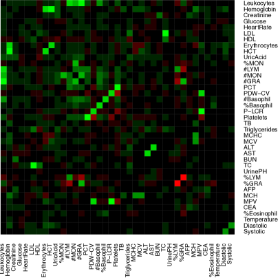
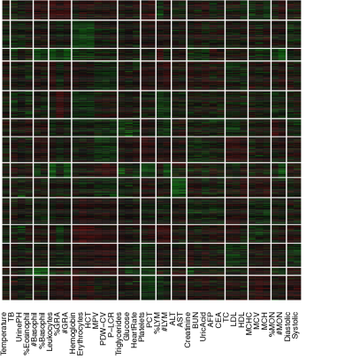
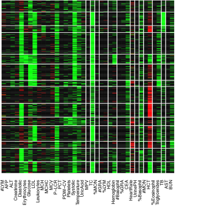
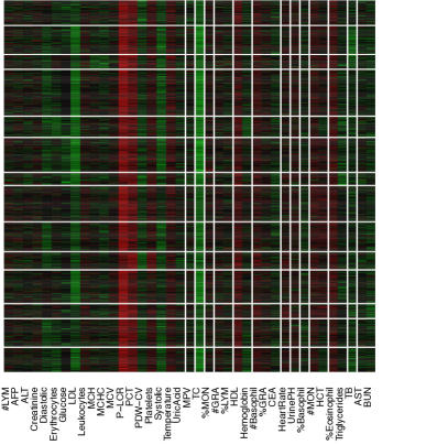
Figure 1: Heatmap of blood test data. In Panel (a), the correlation structure of the testing items is shown with green, black, and red colors indicating positive, negligible and negative correlations. Diagonal entries are set to 0. In Panels (b), (c) and (d), the rows and columns are ordered according to K-means with $K=14$. The columns are the testing items and the rows are patients. In Panel (b), the EHR data is standardized. Green, black and red colors represent values above, near and below the average or the midpoint. In Panel (c), the EHR data is transformed to a categorical matrix based on a trichotomization with respect to a reference range. Green, black and red colors indicate above, within, below the range, respectively. In panel (d), the EHR data is scaled and centered at the midpoint of the reference range (the order of rows and columns is the same as in Panel (c)).

2 Double Feature Allocation Model

DFA can be applied to any categorical matrix. For simplicity, and in anticipation of the application to EHR, we will describe our model for binary and ternary matrices. Let $y_{il}\in\{-1,0,+1\}$ and $z_{ij}\in\{0,1\}$ for $i=1,\dots,n$, $l=1,\dots,q$, and $j=1,\dots,p$. In the EHR dataset, $y_{il}$ denote the observation for patient $i$ for a symptom that can be naturally trichotomized into low ($y_{il}=-1$), normal ($y_{il}=0$) and high ($y_{il}=+1$) levels. Similarly, $z_{ij}$ denotes a symptom that is dichotomized into normal ($z_{ij}=0$) vs abnormal ($z_{ij}=1$) levels. We assume that a patient experiences certain symptoms when he/she has diseases that are related to those symptoms. In other words, the patient-symptom relationships are thought to be generated by two models: a patient-disease model and a symptom-disease model.

2.1 Patient-disease (PD) model

The patient-disease relationships are defined by a binary matrix $\bm{A}=(\alpha_{ik})\in\{0,1\}^{n\times\tilde{K}}$ with $\alpha_{ik}=1$ meaning patient $i$ has disease $k$. We start the model construction assuming a fixed number $\tilde{K}$ of diseases, to be relaxed later (and we reserve the notation $K$ for the relaxation). Conditional on $\tilde{K}$, $\alpha_{ik}$ are assumed to be independent Bernoulli random variables, $\alpha_{ik}\mid\pi_{k}\sim Ber(\pi_{k})$ with $\pi_{k}$ following a conjugate beta prior, $\pi_{k}\sim Beta(m/\tilde{K},1)$. Here $m$ is a fixed hyperparameter. Marginalizing out $\pi_{k}$,

$$p(\bm{A})=\prod_{k=1}^{\tilde{K}}\frac{m\Gamma(r_{k}+\frac{m}{\tilde{K}})\Gamma(n-r_{k}+1)}{\tilde{K}\,\Gamma(n+1+\frac{m}{\tilde{K}})},$$

where $r_{k}=\sum_{i=1}^{n}\alpha_{ik}$ is the sum of the $i$th column of $\bm{A}$.
However, the number of latent diseases is unknown in practice and inference on $\tilde{K}$ is of interest. Let $H_{n}=\sum_{i=1}^{n}1/i$ be the $n$-th harmonic number. Next, take the limit $\tilde{K}\rightarrow\infty$ and remove columns of $\bm{A}$ with all zeros. This step is not trivial and needs careful consideration of equivalence classes of binary matrices; details can be found in Section 4.2 of Griffiths & Ghahramani, (2011). Let $K$ denote the number of non-empty columns. The resulting matrix $\bm{A}$ follows an $\mbox{IBP}(m)$ prior (without a specific column ordering), with probability

$$p(\bm{A})=\frac{m^{K}\exp\{-mH_{n}\}}{K!}\prod_{k=1}^{K}\frac{\Gamma(r_{k})\Gamma(n-r_{k}+1)}{\Gamma(n+1)}.$$ (1)

Since $K$ is random and unbounded, we do not need to specify the number of latent diseases a priori. And with a finite sample size, the number $K$ of non-empty diseases is finite with probability one. See, for example, Griffiths & Ghahramani, (2011) for a review of the IBP, including the motivation for the name based on a generative model. We only need two results that are implied by this generative model. Let $r_{-i,k}$ denote the sum in column $k$, excluding row $i$. Then the conditional probability for $\alpha_{ik}=1$ is

$$p(\alpha_{ik}=1\mid\bm{\alpha}_{-i,k})=r_{-i,k}/n,$$ (2)

provided $r_{-i,k}>0$, where $\bm{\alpha}_{-i,k}$ is the $k$th column of $\bm{A}$ excluding $i$th row. And the distribution of the number of new features (disease) for each row (patient) is $\mbox{Poi}(m/n)$.

2.2 Symptom-disease (SD) model

A disease may trigger multiple symptoms and a symptom may be related to multiple diseases. The SD model allows both. Let $K$ again denote the number of latent diseases. The SD model inherits $K$ from the PD model. For binary symptoms, we generate a binary $(p\times K)$ matrix $\bm{B}=[\beta_{jk}]$, $\beta_{jk}\in\{0,1\}$, from independent Bernoulli distributions, $\beta_{jk}\sim Ber(\rho)$ with $\rho\sim Beta(a_{\rho},b_{\rho})$. Similarly, for ternary symptoms, we generate a $(q\times K)$ ternary matrix $\bm{C}=[\gamma_{lk}]$, $\gamma_{lk}\in\{-1,0,1\}$, from independent categorical distributions $\gamma_{lk}\sim Categ(\bm{\pi})$ with $\bm{\pi}\sim Dir(\phi_{-1},\phi_{0},\phi_{+1})$.

We have considered that $\beta_{jk}\sim Ber(\rho)$ and $\rho\sim Beta(a_{\rho},b_{\rho})$, that is, all binary symptoms (similarly for ternary symptoms) have the same probability of being triggered by any disease a priori, which implies that the $\beta_{jk}$’s are exchangeable across symptoms and diseases. The construction with the unknown hyperparameter $\rho$ allows for automatic multiplicity control (Scott & Berger, , 2010). However, exchangeability does not necessarily hold in all cases. For example, symptoms such as fever are more common than symptoms such as chest pain. If desired, such heterogeneity across symptoms can be incorporated in the proposed model by setting $\beta_{jk}\sim Ber(\rho_{j})$. In addition, the beta prior on $\rho_{j}$ can be adjusted according to the prior knowledge of the importance of each symptom $j$. Letting $\lambda_{j}=\Phi^{-1}(\rho_{j})$ denote a probit transformation of $\rho_{j}$, one can introduce dependence across symptoms by a hierarchical model,

$$\lambda_{j}\mid\lambda,\sigma^{2}\sim N(\lambda,\sigma^{2})$$ (3)

$$\lambda\sim p(\lambda)\propto 1,~{}\sigma^{2}\sim IG(a_{\sigma},b_{\sigma})$$

We explore this approach in a simulation study reported in the Supplementary Material A. A similar strategy can be used to accomodate heterogeneity across diseases, in which case we assume $\beta_{jk}\sim Ber(\rho_{k})$.

Note that $\bm{A}$, $\bm{B}$ and $\bm{C}$ have the same number of columns because they share the same latent diseases. In the language of the Indian restaurant metaphor, each dish (disease) corresponds to a combination of ingredients (symptoms). Some ingredients come at spice levels $\{-1,1\}$, if selected. We have now augmented model (1) by matching each subset of patients, i.e., each disease, with a subset of symptoms defined in $\bm{B}$ and $\bm{C}$. As a result, each disease, or feature, is defined as a pair of random subsets of patients and symptoms, respectively. We therefore refer to the model as double feature allocation (DFA). In this construction we have defined the joint prior of $\bm{A},\bm{B}$ and $\bm{C}$ using the factorization $p(\bm{A},\bm{B},\bm{C})=p(\bm{A})p(\bm{B},\bm{C}\mid\bm{A})$, i.e. first assuming an IBP prior for $\bm{A}$, and then defining a prior on $\bm{B}$ and $\bm{C}$ conditional on $\bm{A}$ (through $K$, the number of columns of $\bm{A}$). In principle, the joint prior can alternatively be factored as $p(\bm{A},\bm{B},\bm{C})=p(\bm{B},\bm{C})p(\bm{A}\mid\bm{B},\bm{C})$, in which case we start the construction with a prior $p(\bm{B},\bm{C})$. However, the categorical nature of $\bm{C}$ complicates this construction and we therefore prefer the earlier factorization.

The main variations in the construction, compared to traditional use of the IBP as prior for a binary matrix, is the use of matched subsets of patients and symptoms for each feature, the mix of binary and categorical items, and the specific sampling model, as it arises in the motivating application.

2.3 Sampling model

Once we generate the PD and SD relationships, the observed data matrix which records the symptoms for each patient is generated by the following sampling models. Let $\bm{\alpha}_{i}$ denote the $i$th row of $\bm{A}$, $\bm{\beta}_{j}$ the $j$th row of $\bm{B}$ as a column vector, and $\bm{\gamma}_{l}$ the $l$th row of $\bm{C}$, written as a column vector. We assume conditionally independent Bernoulli distributions for $z_{ij}$

$$z_{ij}|\bm{\alpha}_{i},\bm{\beta}_{j},\bm{W}_{j},\zeta_{j}\sim Ber\left\{\frac{\exp(\bm{\alpha}_{i}\bm{W}_{j}\bm{\beta}_{j}+\zeta_{j})}{1+\exp(\bm{\alpha}_{i}\bm{W}_{j}\bm{\beta}_{j}+\zeta_{j})}\right\},$$ (4)

with $\bm{W}_{j}=diag(w_{j1},\dots,w_{jK})$ where $w_{jk}$ is constrained to be positive, so that the probability of experiencing symptom $j$ for patient $i$ always increases if a patient has a disease $k$ that triggers the symptom. The parameter $\zeta_{j}$ captures the remaining probability of symptom $j$ that is unrelated to any disease. One could alternatively include the weight already in $\bm{B}$ (and $\bm{C}$). We prefer separating the formation of the random subsets which define the features versus the weights which appear in the sampling model.

Similarly, we assume conditionally independent categorical distributions for $y_{il}$. Let $\mbox{Cat}(\pi_{1},\pi_{2},\pi_{3})$ denote a categorical distribution with probabilities $\pi_{1},\pi_{2},\pi_{3}$ for three outcomes. Also let $\bm{\gamma}_{l}^{+}=I(\bm{\gamma}_{l}=+1)$ and $\bm{\gamma}_{l}^{-}=I(\bm{\gamma}_{l}=-1)$ with $I(\cdot)$ being the element-wise indicator function. We assume

$$y_{il}\mid\bm{\alpha}_{i},\bm{\gamma}_{l},\bm{W}_{l}^{-},\bm{W}_{l}^{+},\eta_{l}^{+},\eta_{l}^{-}\sim\mbox{Cat}\left(Me^{\bm{\alpha}_{i}\bm{W}_{l}^{-}\bm{\gamma}_{l}^{-}+\eta_{l}^{-}},\;M,\;Me^{\bm{\alpha}_{i}\bm{W}_{l}^{+}\bm{\gamma}_{l}^{+}+\eta_{l}^{+}}\right),$$ (5)

with $M$ being the normalization constant, $\bm{W}_{l}^{-}=diag(w_{l1}^{-},\dots,w_{lK}^{-})$ and $\bm{W}_{l}^{+}=diag(w_{l1}^{+},\dots,w_{lK}^{+})$, where $w_{lk}^{-},w_{lk}^{+}$ are also constrained to be positive, and $\eta_{l}^{-}$ and $\eta_{l}^{+}$ have interpretations similar to $\zeta_{j}$.

We complete the model by assigning vague priors on hyperparameters, $\zeta_{j}$, $\eta_{l}^{-}$, $\eta_{l}^{+}\sim N(0,\tau^{2})$ with $\tau=100$ and $w_{jk}$, $w_{lk}^{-}$, $w_{lk}^{+}\sim Gamma(1,\tau_{w})$ with variance $\tau_{w}^{2}=100$. A brief sensitivity analysis for the choice of these hyperparameters is shown in Supplementary Material A.

2.4 Incorporating prior knowledge

Available diagnostic information is easily incorporated in the proposed model. We fix the first $K_{0}$ columns of $\bm{A}$ to represent available diagnoses related to $K_{0}$ known diseases. Specifically, we label the known diseases as $1,\dots,K_{0}$ and set $\alpha_{ik}=1$ if and only if individual $i$ is diagnosed with disease $k$ for $k=1,\dots,K_{0}$. Similarly, known SD relationships are represented by fixing corresponding columns of $\bm{B}$ or $\bm{C}$.

A simple example with 11 patients and 6 ternary symptoms is shown in Figure 2 for illustration. There are 4 diseases, each represented by one color (corresponding to the dashed blocks inside the matrix in Figure 2). Importantly, patients and symptoms can be linked to multiple diseases. For example, patient 9 has both, the blue and the green disease, and symptom 4 can be triggered by either the red or the green disease. Available prior information is incorporated in this example. For instance, if patients 9, 10, 11 are diagnosed with the blue disease, they will be grouped together deterministically (represented by the blue solid line on the side). Likewise, if the yellow disease is known to lead to symptoms 1 and 6, we fix them in the model (represented by the yellow solid lines on the top).

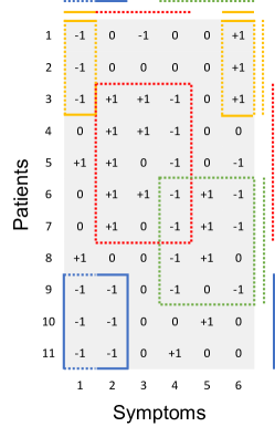
Figure 2: Illustration of DFA for ternary symptoms. The lines on the side/top indicate the grouping of patients/symptoms by diseases. Each disease is represented by one color. Dashed lines are latent whereas solid lines are known.

3 Alternative Interpretations

The proposed DFA is closely related to matrix factorization and random networks. We briefly discuss two alternative interpretations of DFA for the case of the observed data being ternary. Binary outcomes are a special case of ternary outcomes; generalization to more than three categories is straightforward. We use the same toy example as in Section 2.4 to illustrate the alternative interpretations.

Categorical matrix factorization (CMF). DFA can be viewed as a CMF. Merging $\bm{W}$ and $\bm{\gamma}$, model (5) probabilistically factorizes an $(n\times q)$ categorical matrix $\bm{Y}$ into an $(n\times K)$ low-rank binary matrix $\bm{A}$ and an $K\times q$ low-rank nonnegative matrix $\bm{D}=(\delta_{kl})$ where $K<\min(n,q)$, $\delta_{kl}=w_{lk}^{-}\gamma_{lk}^{-}+w_{lk}^{+}\gamma_{lk}^{+}$, $\gamma_{lk}^{-}=I(\gamma_{lk}=-1)$ and $\gamma_{lk}^{+}=I(\gamma_{lk}=+1)$. From (5),

$$\log\{p(y_{il}=y)\}=c+\left\{\begin{array}[]{lcl}\bm{\alpha}_{i}\bm{\delta}_{l}^{-}+\eta_{l}^{-}&\mbox{for}&y=-1\\ \bm{\alpha}_{i}\bm{\delta}_{l}^{+}+\eta_{l}^{+}&\mbox{for}&y=+1\\ 0&\mbox{for}&y=0\end{array}\right.$$ (9)

where $\bm{\delta}_{l}=(\delta_{1l},\dots,\delta_{Kl})^{T}$, $\bm{\delta}_{l}^{-}=\bm{\delta}_{l}\circ I(\bm{\gamma}_{l}=-1)$, $\bm{\delta}_{l}^{+}=\bm{\delta}_{l}\circ I(\bm{\gamma}_{l}=+1)$ with element-wise multiplication $\circ$, and $c=-\log\{\exp(\bm{\alpha}_{i}\bm{\delta}_{l}^{-}+\eta_{l}^{-})+\exp(\bm{\alpha}_{i}\bm{\delta}_{l}^{+}+\eta_{l}^{+})+1\}$. Figure 3 illustrates the factorization. The matrix $\bm{A}$ describes the PD relationships. $\bm{D}^{-}$ and $\bm{D}^{+}$ characterize the SD relationships where $\bm{D}^{-}=\bm{D}\circ I(\bm{C}=-1)$ and $\bm{D}^{+}=\bm{D}\circ I(\bm{C}=+1)$. The number of diseases is less than the number of patients and the number of symptoms.

Edge-labeled random networks. DFA can be also interpreted as inference for a random network with labeled edges. The observed categorical matrix $\bm{Y}$ is treated as a categorical adjacency matrix which encodes a bipartite random network. Patients form one set of nodes and symptoms form another set. The edge labels correspond to the categories in $\bm{Y}$. See the bipartite network on the upper portion of Figure 4 where the two labels ($+1$, $-1$) are respectively represented by arrow heads and flat bars. DFA assumes that the observed bipartite graph is generated from a latent tripartite graph (given in the lower portion of Figure 4). Inference under the DFA model reverses the data generation process. The tripartite graph introduces an additional set of (latent) nodes corresponding to diseases. The edges between patients (symptom) and diseases indicate PD (SD) relationships. Prior PD and SD knowledge is represented by fixing the corresponding edges (solid lines in Figure 4).

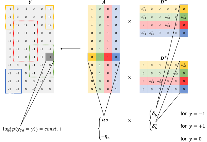
Figure 3: Categorical matrix factorization as an alternative representation of DFA in Figure 2. $\bm{D}^{-}=\bm{D}\circ I(\bm{C}=-1)$ and $\bm{D}^{+}=\bm{D}\circ I(\bm{C}=+1)$. Diseases correspond to the columns of $\bm{A}$ and the rows of $\bm{D}^{-}$ and $\bm{D}^{+}$. They are represented by the same set of colors as in Figure 2.

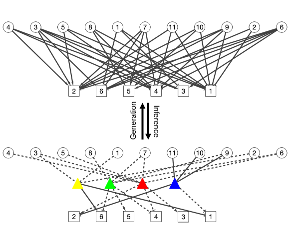
Figure 4: Edge-labeled random networks as an alternative representation of the DFA in Figure 2. The observed bipartite graph (top) is assumed to be generated by the latent tripartite graph (bottom). DFA addresses the inverse problem. Circles are patients, squares are symptoms and triangles are diseases whose colors have the same interpretations as in Figure 2. Dashed lines are latent whereas solid lines are known/observed. An undirected edge connecting patients and diseases is binary. Edges with arrow head or flat bars represent different types of SD relationships.

4 Posterior Inference

The model described in Section 2 is parameterized by

$$\bm{\theta}=\{\bm{A},\bm{B},\bm{C},\{\bm{W}_{j},\zeta_{j}\}_{j=1}^{p},\{\bm{W}^{-}_{l},\bm{W}^{+}_{l},\eta_{l}^{-},\eta_{l}^{+}\}_{l=1}^{q}\}.$$

Posterior inference is carried out by Markov chain Monte Carlo (MCMC) posterior simulation. All parameters except $\bm{A}$ can be updated with simple Metropolis-Hasting transition probabilities. Sampling $\bm{A}$ is slightly more complicated because the dimension of the parameter space can change. We therefore provide details of the transition probability for updating $\bm{A}$. In the implementation, for easier bookkeeping, we set a large upper bound $K_{\vee}=50$ for the number of latent diseases; it is never reached during the course of the MCMC.

MCMC

We use superscript ^(t) to index the state $\bm{\theta}$ across iterations. Initialize $\bm{\theta}^{(0)}$. For $t=0,\dots,T-1$, do

• Update $\bm{A}^{(t+1)}$. We scan through each row, $i=1,\dots,n$, of $\bm{A}=\bm{A}^{(t)}$.

  • Update existing diseases $k=1,\dots,K$. If $\bm{\alpha}_{-i,k}=\bm{0}$, drop disease $k$; otherwise, sample $\alpha_{ik}$ from the full conditional distribution. For $j=0,1$

    $$p(\alpha_{ik}=j\mid\cdot)\propto p(\alpha_{ik}=j\mid\bm{\alpha}_{-i,k})\;p(\bm{z}_{i}\mid\alpha_{ik}=j,\bm{\alpha}_{i,-k},\bm{B},\{\bm{W}_{j},\zeta_{j}\}_{j=1}^{p})\;\times\\ p(\bm{y}_{i}\mid\alpha_{ik}=j,\bm{\alpha}_{i,-k},\bm{C},\{\bm{W}^{-}_{l},\bm{W}^{+}_{l},\eta_{l}^{-},\eta_{l}^{+}\}_{l=1}^{q})\\ =p(\alpha_{ik}=j\mid\bm{\alpha}_{-i,k})\prod_{j=1}^{p}p(z_{ij}\mid\alpha_{ik}=j,\bm{\alpha}_{i,-k},\bm{\beta}_{j},\bm{W}_{j},\zeta_{j})~{}\times\\ \prod_{l=1}^{q}p(y_{il}\mid\alpha_{ik}=j,\bm{\alpha}_{i,-k},\bm{\gamma}_{l},\bm{W}_{l}^{-},\bm{W}_{l}^{+},\eta_{l}^{-},\eta_{l}^{+})$$ (10)

    where the factors in the last equation are defined in (2), (4) and (5), respectively.

  • Propose new diseases. The proposed new diseases are unique to patient $i$ only, i.e., $\alpha_{ik}=1$ and $\bm{\alpha}_{-i,k}=\bm{0}$. We first draw $k^{*}\sim\mbox{Poi}(m/n)$. If $k^{*}=0$, go to the next step. Otherwise, we propose a set of new disease-specific parameters $\bm{\beta}_{k}^{*}=(\beta_{1k}^{*},\dots,\beta_{pk}^{*})^{T}$, $\bm{\gamma}_{k}^{*}=(\gamma_{1k}^{*},\dots,\gamma_{qk}^{*})^{T}$, $\{w_{jk}^{*}\}_{j=1}^{p}$, $\{w_{lk}^{-*},w_{lk}^{+*}\}_{l=1}^{q}$ for $k=K+1,\dots,K+k^{*}$ from their respective prior distributions. We accept the new disease(s) and the disease-specific parameters, with probability

    $$\min\left\{1,\frac{\prod_{j=1}^{p}p(z_{ij}\mid\bm{\alpha}_{i}^{*},\bm{\beta}_{j}^{*},\bm{W}_{j}^{*},\zeta_{j})}{\prod_{j=1}^{p}p(z_{ij}\mid\bm{\alpha}_{i}^{(t)},\bm{\beta}_{j}^{(t)},\bm{W}_{j}^{(t)},\zeta_{j})}\,\frac{\prod_{l=1}^{q}p(y_{il}\mid\bm{\alpha}_{i}^{*},\bm{\gamma}_{l}^{*},\bm{W}_{l}^{-*},\bm{W}_{l}^{+*},\eta_{l}^{-},\eta_{l}^{+})}{\prod_{l=1}^{q}p(y_{il}\mid\bm{\alpha}_{i}^{(t)},\bm{\gamma}_{l}^{(t)},\bm{W}_{l}^{-(t)},\bm{W}_{l}^{+(t)},\eta_{l}^{-},\eta_{l}^{+})}\,\right\},$$

    where $\bm{\alpha}_{i}^{*}=(\bm{\alpha}_{i}^{(t)},1,\dots,1)$, $\bm{\beta}_{j}^{*}=(\bm{\beta}_{j}^{(t)T},\beta_{j,K+1}^{*},\dots,\beta_{j,K+k^{*}}^{*})^{T}$, $\bm{\gamma}_{l}^{*}=(\bm{\gamma}_{l}^{(t)T},\gamma_{l,K+1}^{*},\dots,\gamma_{l,K+k^{*}}^{*})^{T}$, $\bm{W}_{j}^{*}=blkdiag(\bm{W}_{j}^{(t)},w_{j,K+1}^{*},\dots,w_{j,K+k^{*}}^{*})$, $\bm{W}_{l}^{-*}=blkdiag(\bm{W}_{l}^{-(t)},w_{l,K+1}^{-*},\dots,w_{l,K+k^{*}}^{-*})$ and $\bm{W}_{l}^{+*}=blkdiag(\bm{W}_{l}^{+(t)},w_{l,K+1}^{+*},\dots,w_{l,K+k^{*}}^{+*})$. Note that the acceptance probability only involves the likelihood ratio because prior and proposal probabilities cancel out. If the new disease is accepted, we increase $K$ by $k^{*}$.

• Update all other parameters in $\bm{\theta}^{(t+1)}$ using Metropolis-Hasting transition probabilities.

To summarize the posterior distribution based on the the MCMC simulation output, we proceed by first calculating the maximum a posteriori (MAP) estimate $\widehat{K}$ from the marginal posterior distribution of $K$. Conditional on $\widehat{K}$, we find the least squares estimator $\widehat{\bm{A}}$ by the following procedure (Dahl, , 2006; Lee et al. , , 2015). For any two binary matrices $\bm{A},\bm{A}^{\prime}\in\{0,1\}^{n\times\widehat{K}}$, we define a distance $d(\bm{A},\bm{A}^{\prime})=\min_{\pi}\mathcal{H}(\bm{A},\pi(\bm{A}^{\prime}))$ where $\pi(\bm{A}^{\prime})$ denotes a permutation of the columns of $\bm{A}^{\prime}$ and $\mathcal{H}(\cdot,\cdot)$ is the Hamming distance of two binary matrices. A point estimate $\widehat{\bm{A}}$ is then obtained as

$$\widehat{\bm{A}}=\arg\min_{\bm{A}^{\prime}}\int d(\bm{A},\bm{A}^{\prime})dp(\bm{A}\mid\bm{Z},\bm{Y},\widehat{K}).$$

Both, the integral as well as the optimization can be approximated using the available Monte Carlo MCMC samples, by carrying out the minimization over $\bm{A}^{\prime}\in\{\bm{A}^{(t)};\;t=1,\ldots,T\}$ and by evaluating the integral as Monte Carlo average. The posterior point estimators of other parameters in $\bm{\theta}$ are obtained as posterior means conditional on $\widehat{\bm{A}}$. We evaluate the posterior means using the posterior Monte Carlo samples.

The described MCMC simulation is practicable up to moderately large $n$, including $n=1000$ in the motivating EHR application. For larger sample sizes, different posterior simulation methods are needed. We briefly discuss some suggestions in Section 7, and in Supplementary Material A.

5 Simulation Study

We consider two simulation scenarios. In both scenarios, we generate the patient-disease matrix $\bm{A}$ from an IBP($m$) model with $m=1$ and sample size $n=300$. The resulting matrix $\bm{A}$ has $K=6$ columns and $n=300$ rows, displayed in Figure 5(b). Given $K=6$, we generate a binary symptom-disease matrix $\bm{B}\in\{0,1\}^{p\times K}$ and a categorical symptom-disease matrix $\bm{C}\in\{-1,0,1\}^{q\times K}$ with $p=q=24$ in the following manner. We first set $\beta_{jk}=1$ for $k=1,\dots,6$ and $j=4(k-1)+1,\dots,4k$, $\gamma_{lk}=-(-1)^{k}$ for $k=1,\dots,6$ and $l=4(k-1)+1,\dots,4k$. We then randomly change 10% of the zero entries in $\bm{B}$ to 1 and 10% of the zero entries in $\bm{C}$ to +1 or -1. The resulting matrices $\bm{B}$ and $\bm{C}$ are shown in Figures 5(c) and 5(d).

In Scenario I, the observations $\bm{Z}$ and $\bm{Y}$ are generated from the sampling model i.e. equations (4) and (5). To mimic the Chinese EHR data, we assume that we have diagnoses for the first disease and that we know the related symptoms for the first disease. In the model, we therefore fix the first column of $\bm{A}$, $\bm{B}$ and $\bm{C}$ to the truth. In addition, we assume that we have partial information about the second latent disease: the symptom-disease relationships are known, but no diagnostic information is available. Accordingly, we will fix the second columns of $\bm{B}$ and $\bm{C}$, but leave the second column of $\bm{A}$ as unknown parameters. We ran the MCMC algorithm described in Section 4 for 5,000 iterations, which took $<5$ minutes on a desktop computer with a 3.5 GHz Intel Core i7 processor. The first half of the iterations are discarded as burn-in and posterior samples are retained at every 5th iteration afterwards.

Inference summaries are reported in Figure 5. Figure 5(a) shows the posterior distribution of the number $K$ of latent diseases. The posterior mode occurs at the true value $\widehat{K}=6$. Conditional on $\widehat{K}$, the posterior point estimate $\widehat{\bm{A}}$ is displayed in Figure 5(e) with mis-allocation rate $\mathcal{H}(\widehat{\bm{A}},\bm{A})/(n\cdot K)=3\%$. Conditional on $\widehat{\bm{A}}$, the point estimates $\widehat{\bm{B}}$ and $\widehat{\bm{C}}$ are provided in Figures 5(f) and 5(g). The similarity between the heatmaps of the simulation truth and estimates indicates an overall good recovery of the signal. The error rates in estimating $\bm{B}$ and $\bm{C}$ are 0% and 2%, respectively. We repeat this simulation 50 times. In 96% of the repeat simulations, we correctly identify the number $K$ of latent diseases; in the remaining 4%, it is overestimated by 1. When $K$ is correctly estimated, the average mis-allocation rate, error rates for $\bm{B}$ and $\bm{C}$ are 3%, 1% and 1% with standard deviation 0.5%, 1% and 1%, respectively. We provide addtional simulation studies in Supplementary Material A to investigate the performance of DFA with different hyperparameters and with the alternative prior that was introduced in (3).

(a) Posterior distribution of number of diseases

(b) True $\bm{A}$

(c) True $\bm{B}$

(d) True $\bm{C}$

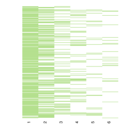
(e) Estimated $\widehat{\bm{A}}$

(f) Estimated $\widehat{\bm{B}}$

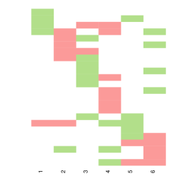
(g) Estimated $\widehat{\bm{C}}$

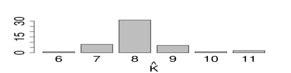
(h) $\widehat{K}$ across 50 simulations.

Figure 5: Simulation truth and posterior estimates. Panels (a)-(g) are from Scenario I and Panel (h) is from Scenario II. In the heatmaps, green cells represent 1, white cells 0 and red cells -1.

In Scenario II, we use a different simulation truth and generate data $\{\widetilde{\bm{Z}},\widetilde{\bm{Y}}\}$ from latent factor models

$$\widetilde{\bm{Z}}=\bm{\Phi}\bm{\Lambda}_{z}+\bm{E}_{z}\mbox{~{}~{}and~{}~{}}\widetilde{\bm{Y}}=\bm{\Phi}\bm{\Lambda}_{y}+\bm{E}_{y}$$

with latent factor matrix $\bm{\Phi}=\bm{A}\circ\widetilde{\bm{\Phi}}$ and loading matrices $\bm{\Lambda}_{z}=\bm{B}\circ\widetilde{\bm{\Lambda}}_{z},\bm{\Lambda}_{y}=\bm{C}\circ\widetilde{\bm{\Lambda}}_{y}$ where $\bm{A},\bm{B},\bm{C}$ are the same as in Scenario I. The elements of $\widetilde{\bm{\Phi}},\widetilde{\bm{\Lambda}}_{z},\widetilde{\bm{\Lambda}}_{y}$ are i.i.d. $Unif(0,4)$ and the errors are i.i.d. standard normal. We then threshold $\widetilde{\bm{Z}}$ and $\widetilde{\bm{Y}}$ to obtain $\bm{Z}$ and $\bm{Y}$ at different levels $t>0$:

$$z_{ij}=\left\{\begin{array}[]{lcl}1&\mbox{if}&\tilde{z}_{ij}>t\\ 0&\mbox{if}&\tilde{z}_{ij}\leq t\end{array}\right.\mbox{~{}~{}and~{}~{}}y_{il}=\left\{\begin{array}[]{lcl}+1&\mbox{if}&\tilde{y}_{il}>t\\ 0&\mbox{if}&|\tilde{y}_{il}|\leq t\\ -1&\mbox{if}&\tilde{y}_{il}<-t.\end{array}\right.$$

We applied DFA to $\{\bm{Z},\bm{Y}\}$ using different values of the threshold $t\in\{1,2,3,4,5\}$. Also, we include no known diseases. Performance deteriorates as $t$ grows. DFA tends to overestimate the number $\widehat{K}$ of latent factors by 1 to 3 extra factors. After removing those extra factors, the mis-allocation rate $\mathcal{H}(\widehat{\bm{A}},\bm{A})/(n\cdot K)$ is between 9% and 19%. And the error rates for $\widehat{\bm{B}}$ and $\widehat{\bm{C}}$ are between 1% and 17%.

For comparison, we implemented inference also under the sparse latent factor model (SLFM, Ročková & George, 2016) to $\{\widetilde{\bm{Z}},\widetilde{\bm{Y}}\}$. SLFM assumes a sparse loading matrix and unstructured latent factors. Therefore, we only report performance in recovering the sparse structure $\bm{B}$ and $\bm{C}$ of the loading matrices $\bm{\Lambda}_{z}$ and $\bm{\Lambda}_{y}$. The penalty parameter $\lambda_{0}$ of SLFM is chosen in an “oracle” way: we fit SLFM with a range of $\lambda_{0}$ values and select $\lambda_{0}$ that yields the best performance given the simulation truth. The resulting error rates in estimating $\bm{B}$ and $\bm{C}$ are 11% and 10%, comparable to those of DFA (keeping in mind the oracle choice of $\lambda_{0}$).

We repeat the experiment 50 times for $t=3$. The estimated $\widehat{K}$ across 50 simulations are plotted in Figure 5(h). We observe that DFA tends to overestimate $K$ when model is misspecified. We report the performance of estimating $\widehat{\bm{B}}$ and $\widehat{\bm{C}}$ based on the best subset of columns. The mean (standard deviation) error rates in estimating $\bm{B}$ and $\bm{C}$ are 8% (4%) and 9% (3%), respectively. SLFM has slightly higher error rates, 12% (1%) and 11% (1%).

6 Phenotype Discovery with EHR Data

6.1 Data and preprocessing

We implement latent disease mining for the EHR data introduced in Section 1.1. Using the reference range for each test item, we define a symptom if the value of an item falls beyond the reference range. Some symptoms are binary in nature, e.g. low density lipoprotein is clinically relevant only when it is higher than normal range. Other symptoms are inherently ternary, e.g. heart rate is symptomatic when it is too high or too low. The 39 testing items are listed in Table 1 where we also indicate which items give rise to a binary or ternary symptom.

We extract diagnostic codes for diabetes from the sections “medical history” and “other current diseases” in the physical examination form. A subject is considered as having diabetes if it is listed in either of the two sections. There are 36 patients diagnosed with diabetes. We fix the first column of $\bm{A}$ in the PD model according to the diabetes diagnosis. Moreover, it is known that diabetes is clinically associated with high glucose level. We incorporate this prior information by fixing the corresponding entry in the first column of $\bm{C}$ in the SD model.

There is additional prior knowledge about symptom-disease relationships. Creatinine, a waste product from muscle metabolism, is controlled by the kidneys to stay within a normal range. Creatinine has therefore been found to be a reliable indicator of kidney function. Elevated creatinine level suggests damaged kidney function or kidney disease. Blood urea nitrogen (BUN) level is another indicator of kidney function. Like creatinine, urea is also a metabolic byproduct which can build up if kidney function is impaired. We fix the two entries (corresponding to creatinine and BUN) of the second column of $\bm{C}$ to 1 and the rest to 0. With this prior knowledge, we interpret the second latent disease as kidney disease. Likewise, it is known that elevated systolic blood pressure and diastolic blood pressure are indicators of hypertension, and abnormal levels of total bilirubin (TB), aspartate aminotransferase (AST) and alanine aminotransferase (ALT) are indicators of liver diseases. We fix the corresponding entries of the third and fourth column of $\bm{B}$ and $\bm{C}$, and interpret the third latent disease as hypertension and the fourth latent disease as liver disease.

To comply with Chinese policy, we report inference for data preprocessed by a Generative Adversarial Network (GAN, Goodfellow et al. , 2014), which replicates the distribution underlying the raw data. GAN is a machine learning algorithm which simultaneously trains a generative model and a discriminative model on a training dataset (in our case, the raw EHR dataset). The generative model simulates a hypothetical repetition of the training data, which is then combined with the original training data to form a merged data set. Meanwhile, the discriminative model tries to distinguish between original data and simulations in the merged data set. During training, the generative model uses gradient information from the discriminative model to produce better simulations. Training continues until the discriminative model can no longer distinguish. After training, the generative model can be used to generate an arbitrary number of simulations which are similar in distribution to the original dataset. Any statistical inference in the original data and the replicated data is identical to the extent to which it relies on low dimensional marginal distributions. In our case, we generate a simulated dataset of the same size as the raw EHR dataset and then discretize it using the reference range. A similar approach has been used in Ni et al. , (2018).

6.2 Results and interpretations

We ran the MCMC algorithm described in Section 4 for 50,000 iterations. The first half of the iterations are discarded as burn-in and posterior samples are retained at every 5th iteration thereafter. Goodness-of-fit and MCMC convergence diagnostics show adequate fit and no evidence for lack of convergence (Supplementary Material B). Posterior probabilities for the number $K$ of latent diseases are $p(K=14\mid data)=0.69$ and $p(K=15\mid data)=0.24$, respectively, i.e., the maximum a posteriori (MAP) estimate is $\widehat{K}=14$. This includes the 4 a priori known diseases as well as 10 newly discovered latent diseases.

Conditional on $\widehat{K}$, the posterior estimates of the PD and SD models are shown as a heatmap in Figure 7 with green, black and red cells representing 1, 0 and -1, respectively. The nature of the figure as a single heatmap with two blocks, for PD and SD, respectively, highlights again the nature of the model as a “double” feature allocation with matching subsets of patients and symptoms. The model allocates both, patients and symptoms, to latent diseases. As mentioned before, DFA can also be interpreted as an edge-labeled network. We show the same results as in the heatmap as a bipartite graph in Figure 8(a). The full inferred model would be a tripartite network, as in the bottom portion of Figure 4. However, we omit the patient nodes in Figure 8(a) , lest the figure would be overwhelmed by the patient nodes. Instead, we summarize the patient-disease relationships by specifying the font size of the disease node (triangle, purple font) proportional to the number of linked patients. Latent diseases are labeled by numbers and a priori known diseases are labeled by name. Symptoms are shown in black font, with lines showing the links to diseases. Dashed lines are symptom-disease relationships that are inferred from the data whereas solid lines are fixed by prior knowledge. Black lines indicate that symptoms are binary. Red (blue) lines indicate suppression (enhancement) relative to the normal range. Line widths are proportional to the posterior probabilities of edge inclusion.

We find 239 patients with impaired kidney function or kidney disease, 183 patients with hypertension and 93 patients with liver disease. The prevalence of kidney disease is slightly higher than the national average 16.9% (Zhang et al. , , 2012) probably because of the elderly patient population in this study. We caution that the estimated prevalence from our analysis should be viewed as an estimate for the lower bound of the actual prevalence in the target patient population because we are not explicitly addressing confounders such as treatment. For example, our estimated hypertension prevalence (18.3%) is much lower than the national average 57.3% (Zhang et al. , , 2017), probably simply due to successful and widely available treatment. Individuals who were previously diagnosed with hypertension and comply with the prescribed medication may not show any symptom (high blood pressure) in the physical examination.

We identify additional 10 latent diseases with prevalence of 493, 218, 192, 174, 114, 82, 64, 24, 15, and 15 patients. Some of the latent diseases are quite interesting. Latent disease 1 is lipid disorder, associated with high total cholesterol (TC), triglycerides and low density lipoprotein (LDL). Cholesterol is an organic molecule carried by lipoproteins. LDL is one type of such lipoproteins, commonly referred to as “bad” cholesterol. At normal levels, TC and LDL are essential substances for the body. However, high levels of TC and LDL put patients at increased risk for developing heart disease and stroke. Triglycerides are a type of fat found in the blood which are produced by the body from excessive carbohydrates and fats. Like cholesterol, triglycerides are essential to life at normal levels. However, a high level is associated with an increased chance for heart disease.

Latent disease 3 can be characterized as thrombocytopenia-like disease which causes low count of platelets, decreased plateletcrit (PCT) and coefficient of variation of platelet distribution (PDW-CV), and increased mean platelet volume (MPV). Patients with low platelets may not be able to stop bleeding after injury. In more serious cases, patients may bleed internally which is a life-threatening condition.

Latent disease 4 is a polycythemia-like disease, associated with elevated mean corpuscular hemoglobin concentration (MCHC), hemoglobin, erythrocytes and hematocrit (HCT). These symptoms match exactly the symptoms of polycythemia, a disease that gives rise to an increased level of circulating red blood cells in the bloodstream. Polycythemia can be caused intrinsically by abnormalities in red blood cell production or by external factors such as chronic heart diseases.

Interestingly, like latent disease 4, latent disease 6 is also related to hemoglobin, erythrocytes and HCT. However, it is linked with a decrease in these levels; hence we refer to the disease as anemia.

Latent disease 7 suggests bacterial infection with increased leukocytes, granulocytes (GRA) and heart rate, and decreased monocytes (MON) and lymphocytes (LYM). The immune system, specifically the bone marrow, produces more GRA and leukocytes to fight a bacterial infection. As a result, the relative abundance of MON and LYM decreases.

Relatedly, latent disease 8 may be caused by viral infection. Viruses can disrupt the function of bone marrow which leads to low levels of leukocytes and GRA, and high levels of LYM.

Latent disease 9 is related to allergy with abnormal basophil, GRA and LYM.

Latent disease 10 suggests that a small group of patients may have malnutrition, which is linked with low blood glucose and anemia-like symptoms such as low corpuscular volume (MCV) and corpuscular hemoglobin (MCH).

Such automatically generated inference on latent disease phenotypes is of high value for routine health exams. It helps the practitioners to focus resources on specific patients and suggests meaningful additional reports. Inference in the statistical model can of course not replace clinical judgment and needs further validation. But it can provide an important decision tool to prioritize resources, especially for areas with limited medical support such as the areas where our data are collected from.

We remark that although there are clear interpretations for most latent diseases found by DFA, latent diseases 2 and 5 cannot easily be interpreted as specific diseases. Latent disease 2 is associated with 12 symptoms, which is likely beyond the number of symptoms of any single disease. Most of the symptoms, such as platelets, leukocytes and lymphocytes, are due to a weak immune system. Considering the elderly population of this dataset, aging could be a reasonable cause. Decreased heart rate and low glucose level can also be explained by aging. Latent disease 5 is linked with elevated systolic blood pressure and glucose. While those two symptoms may not be simultaneously linked to the same disease, their co-appearance should not be too surprising because the co-existence of hypertension and diabetes (to which blood pressure and glucose are known to be linked) is quite common (De Boer et al. , , 2017).

We report the estimation of $\{\bm{W}_{j},\zeta_{j}\}_{j=1}^{p}$ and $\{\bm{W}^{-}_{l},\bm{W}^{+}_{l},\eta_{l}^{-},\eta_{l}^{+}\}_{l=1}^{q}$ in Supplementary Material B. The estimated baseline weights $\zeta_{j},\eta_{l}^{-},\eta_{l}^{+}$ are significantly smaller than disease-related weights $\bm{W}_{j},\bm{W}^{-}_{l},\bm{W}^{+}_{l}$.

6.3 A Web application for disease diagnosis

A good user interface is critical to facilitate the implementation of the proposed approach in the decision process of healthcare providers, and for broad application. Using the R package shiny (Chang et al. , , 2015), we have created an interactive web application (available at https://nystat3.shinyapps.io/Rshiny/). The application displays disease diagnosis recommendations for de-identified patients selected by the user. We show the application for two patients in Figure 6.

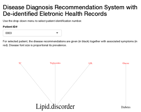
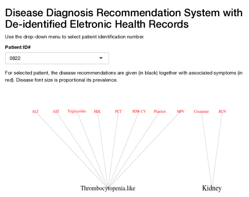
Figure 6: Two examples of the R Shiny web application. Each example is for one patient. The application interactively displays disease diagnosis recommendations for de-identified patients selected by the user.

6.4 Comparison

As a comparison with results under alternative approaches, we consider inference under SLFM, applied directly to the blood test results, without converting to binary or ternary symptoms. The tuning parameter $\lambda_{0}$ was set to 1 to approximately match the number of latent diseases found by DFA. SLFM implements inference on sparse symptom-disease relationships as shown in Figure 8(b). Although there is no known truth for symptom-disease relationships, it is difficult to interpret certain links. While uric acid may play some role in certain diseases, we do not expect it to be related to 5 out of 12 latent diseases. In addition, both latent diseases 5 and 6 are related to platelets only, which should be collapsed into one disease. We also ran LSFM with larger $\lambda_{0}$ but found similar results. For example, when $\lambda_{0}=10$, SLFM identifies 20 latent diseases, 17 of which are associated with uric acid. These somewhat surprising results may be due to the assumption of normality and linearity of SLFM, and taking no advantage of prior information.

Next we apply SLFM to the EHR data that are scaled and centered at the midpoint of each reference range. Choosing $\lambda_{0}=13$, the algorithm found 10 latent diseases whose relationships with symptoms are depicted in Figure 8(c). Some findings are consistent with ours. For example, disease 3 here is similar to disease 1 from DFA. Both are related to LDL and TC. Likewise, disease 2 is similar to disease 4 from DFA. But some findings remain difficult to interpret. Six diseases are associated with only one symptom. For instance, disease 10 is linked to only MPV. However, high or low MPV alone is not of any clinical importance. It is only of concern if other platelet-related measurements are also out of their normal ranges. This synergy is well captured by DFA (via disease 3).

As already briefly commented in Section 1, graphical models may be also employed for finding hidden structures of the symptoms. We run a birth-death MCMC algorithm (available in the R package BDgraph, Mohammadi & Wit, 2015) for 50,000 iterations to learn a Bayesian graphical model. A point estimate is shown in Figure 8(d). Symptoms that form cliques of size greater than 3 are marked by circles. Some of the findings are consistent with those by the DFA. As an illustration, the clique of TC, triglycerides, LDL and HDL is very similar to latent disease 1 in Figure 8(a). However, although graphical models can find latent patterns that are not immediately obvious in the correlation structure (Figure 1a), like SLFM, it lacks inference on patient-disease relationships. Moreover, identifying cliques or other graph summaries as disease is an arbitrary choice.

Figure 7: EHR data. The heatmap on top shows the estimated patient-disease relationships $\widehat{\bm{A}}$. The bottom part of the double heatmap shows the estimated symptom-disease relationships $\widehat{\bm{B}},\widehat{\bm{C}}$ with green, black and red cells representing 1, 0 and -1, respectively. The columns correspond to diseases and the rows are patients (top portion) and symptoms (bottom portion).

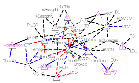
(a) SD bipartite network from DFA

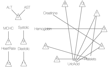
(b) SD bipartite network from SLFM

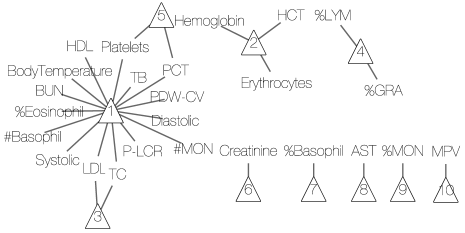
(c) SD bipartite network from SLFM with prior information

(d) Symptom network from BDgraph

Figure 8: EHR data analysis. (a) Bipartite network for symptom-disease relationships from DFA. The diseases are represented by triangles with the font size proportional to its popularity (i.e. the number of patients having the disease). Latent diseases are represented by the numbers (10 latent diseases in total). The symptoms are given in black font and their links to each disease are represented by the lines. Dashed lines are symptom-disease relationships inferred from the data whereas solid lines are fixed by prior knowledge. Black lines indicate the symptoms are binary. Red (blue) lines indicate the disease causes the symptom to be lower (higher) than normal range. The line width is proportional to its posterior probability of inclusion. (b) Bipartite network for symptom-disease relationships from SLFM. Latent diseases are represented by triangles (8 latent diseases in total). (c) Network for symptom-disease relationships from BDgraph. There are 5 cliques of length greater than 3 in total. The symptoms that form those cliques are represented by circles.

7 Discussion

We have developed a DFA model for discovery of latent diseases in EHR data. DFA can be equivalently viewed as categorical matrix factorization or as inference in edge-labeled random networks. In the EHR data analysis, it is important to include available diagnostic information and other prior knowledge, which greatly facilitates identification of latent diseases. We found that the prevalence of damaged kidney function in our dataset is comparable with, but slightly higher than the regional average. We also found 10 latent diseases that are related to lipid disorder, thrombocytopenia, polycythemia, anemia, bacterial and viral infections, allergy, and malnutrition. Finally, although the proposed DFA model is specifically designed for disease mining, it could find broader applications in various areas such as education and psychology (Chen et al. , , 2015; Chen et al. , , 2018).

As demonstrated in Section 6, inference under the DFA model includes inference on patient-disease relationships. Neither of the alternative approaches, SLFM or graphical models, include this capability. Knowing patient-disease relationships is crucial in prioritizing limited medical resources. The proposed inference for the DFA is fully Bayesian. Therefore, it outputs not only point estimates but also the associated uncertainties through, e.g., the posterior probability of symptom-disease relationships (reflected by the line width in Figure 8(a)). SLFM is implemented using an Expectation-Maximization (EM) algorithm. It can quickly get point estimates, but does not include uncertainties.

One of our preprocessing steps is discretizing the original observations into binary or ternary variables. The main rationale of discretization is two-fold: (1) the reference range of each test is naturally incorporated; (2) it reduces sensitivity to noise, outliers and distributional assumptions. The downside of discretization, however, is a potential loss of information, which can mitigated by increasing the number of categories of the discretization.

Although EHR often involves analysis of big datasets, scalability to large sample size is not the focus of this paper. We focus on inference for data from a more narrowly restricted subset equivalent to about a week worth of data. We have shown that such data already allows meaningful inference on latent diseases. If desired and reasonable, the same approach could of course be used for larger data sets, but would likely need to be combined with model extensions to allow for changes in the latent structure, i.e., disease patterns, across different towns, times and other important factors. Implementation needs computationally efficient algorithms for posterior inference such as consensus Monte Carlo. In Supplementary Material A, we summarize a small simulation study assessing the performance of a consensus Monte Carlo algorithm for larger sample sizes. Computation time for a sample size of 15,000 is under 5 minutes, and summaries of the estimation performance remain comparable to the MCMC algorithm on small datasets.

Due to the conditional independence assumption of the sampling model in (4) and (5), given the model parameters, the proposed DFA can be easily extended to inference on datasets with missing values by simply ignoring factors in the likelihood that involve missing values; similar approaches have been studied extensively in the matrix completion and collaborative filtering literature. One caveat is that it implicitly makes a missing completely at random assumption. The EHR dataset that we considered here does not have massive missingness. However, more careful consideration of missingness is needed for application to EHR data with possibly informative missingness. For instance, with laboratory test results, a missing test item may suggest a normal result, if one assumed that a test would only be ordered if based on other symptoms an abnormal level were expected.

References

- Barrios et al. , (2013) Barrios, Ernesto, Lijoi, Antonio, Nieto-Barajas, Luis E., & Prünster, Igor. 2013. Modeling with Normalized Random Measure Mixture Models. Statist. Sci., 28(3), 313–334.
- Bhattacharya & Dunson, (2011) Bhattacharya, Anirban, & Dunson, David B. 2011. Sparse Bayesian infinite factor models. Biometrika, 98, 291–306.
- Broderick et al. , (2013) Broderick, Tamara, Jordan, Michael I, & Pitman, Jim. 2013. Cluster and feature modeling from combinatorial stochastic processes. Statistical Science, 28, 289–312.
- Campbell et al. , (2018) Campbell, Trevor, Cai, Diana, & Broderick, Tamara. 2018. Exchangeable trait allocations. Electronic Journal of Statistics, 12(2), 2290–2322.
- Chang et al. , (2015) Chang, Winston, Cheng, Joe, Allaire, JJ, Xie, Yihui, & McPherson, Jonathan. 2015. shiny: Web Application Framework for R. R package version 0.12.2.
- Chen et al. , (2018) Chen, Yinghan, Culpepper, Steven Andrew, Chen, Yuguo, & Douglas, Jeffrey. 2018. Bayesian estimation of the DINA Q matrix. Psychometrika, 83(1), 89–108.
- Chen et al. , (2015) Chen, Yunxiao, Liu, Jingchen, Xu, Gongjun, & Ying, Zhiliang. 2015. Statistical analysis of Q-matrix based diagnostic classification models. Journal of the American Statistical Association, 110(510), 850–866.
- Dahl, (2006) Dahl, D. B. 2006. Model-Based Clustering for Expression Data via a Dirichlet Process Mixture Model. In: Vannucci, Marina, Do, Kim-Anh, & Müller, Peter (eds), Bayesian Inference for Gene Expression and Proteomics. Cambridge University Press.
- De Boer et al. , (2017) De Boer, Ian H, Bangalore, Sripal, Benetos, Athanase, Davis, Andrew M, Michos, Erin D, Muntner, Paul, Rossing, Peter, Zoungas, Sophia, & Bakris, George. 2017. Diabetes and hypertension: a position statement by the American Diabetes Association. Diabetes Care, 40(9), 1273–1284.
- Dobra et al. , (2011) Dobra, Adrian, Lenkoski, Alex, & Rodriguez, Abel. 2011. Bayesian inference for general Gaussian graphical models with application to multivariate lattice data. Journal of the American Statistical Association, 106(496), 1418–1433.
- Favaro & Teh, (2013) Favaro, Stefano, & Teh, Yee Whye. 2013. MCMC for Normalized Random Measure Mixture Models. Statist. Sci., 28(3), 335–359.
- Goodfellow et al. , (2014) Goodfellow, Ian, Pouget-Abadie, Jean, Mirza, Mehdi, Xu, Bing, Warde-Farley, David, Ozair, Sherjil, Courville, Aaron, & Bengio, Yoshua. 2014. Generative Adversarial Nets. Pages 2672–2680 of: Advances in Neural Information Processing Systems.
- Green & Thomas, (2013) Green, Peter J., & Thomas, Alun. 2013. Sampling decomposable graphs using a Markov chain on junction trees. Biometrika, 100(1), 91–110.
- Griffiths & Ghahramani, (2006) Griffiths, Thomas L., & Ghahramani, Zoubin. 2006. Infinite latent feature models and the Indian buffet process. Pages 475–482 of: Weiss, Y., Schölkopf, B., & Platt, J. (eds), Advances in Neural Information Processing Systems 18. MIT Press, Cambridge, MA.
- Griffiths & Ghahramani, (2011) Griffiths, Thomas L, & Ghahramani, Zoubin. 2011. The Indian buffet process: An introduction and review. Journal of Machine Learning Research, 12(Apr), 1185–1224.
- Guo, (2013) Guo, Lei. 2013. Bayesian Biclustering on Discrete Data: Variable Selection Methods. Ph.D. thesis, Harvard University.
- Halpern et al. , (2016) Halpern, Yoni, Horng, Steven, Choi, Youngduck, & Sontag, David. 2016. Electronic medical record phenotyping using the anchor and learn framework. Journal of the American Medical Informatics Association, 23(4), 731–740.
- Hartigan, (1972) Hartigan, John A. 1972. Direct clustering of a data matrix. Journal of the American Statistical Association, 67(337), 123–129.
- Henderson et al. , (2017) Henderson, Jette, Ho, Joyce C, Kho, Abel N, Denny, Joshua C, Malin, Bradley A, Sun, Jimeng, & Ghosh, Joydeep. 2017. Granite: Diversified, sparse tensor factorization for electronic health record-based phenotyping. Pages 214–223 of: Healthcare Informatics (ICHI), 2017 IEEE International Conference on. IEEE.
- Lau & Green, (2007) Lau, John W, & Green, Peter J. 2007. Bayesian model-based clustering procedures. Journal of Computational and Graphical Statistics, 16(3), 526–558.
- Lauritzen, (1996) Lauritzen, Steffen L. 1996. Graphical models. Vol. 17. Oxford: Clarendon Press.
- Lee et al. , (2015) Lee, Juhee, Müller, Peter, Gulukota, Kamalakar, & Ji, Yuan. 2015. A Bayesian feature allocation model for tumor heterogeneity. Ann. Appl. Stat., 9(2), 621–639.
- Li, (2005) Li, Tao. 2005. A general model for clustering binary data. Pages 188–197 of: Proceedings of the eleventh ACM SIGKDD international conference on Knowledge discovery in data mining. ACM.
- Meeds et al. , (2007) Meeds, Edward, Ghahramani, Zoubin, Neal, Radford M, & Roweis, Sam T. 2007. Modeling dyadic data with binary latent factors. Pages 977–984 of: Advances in Neural Information Processing Systems.
- Miettinen et al. , (2008) Miettinen, Pauli, Mielikäinen, Taneli, Gionis, Aristides, Das, Gautam, & Mannila, Heikki. 2008. The discrete basis problem. IEEE Transactions on Knowledge and Data Engineering, 20(10), 1348–1362.
- Miller & Harrison, (2018) Miller, Jeffrey W., & Harrison, Matthew T. 2018. Mixture Models With a Prior on the Number of Components. Journal of the American Statistical Association, 113(521), 340–356.
- Mohammadi & Wit, (2015) Mohammadi, Abdolreza, & Wit, Ernst C. 2015. BDgraph: an R package for Bayesian structure learning in graphical models. arXiv preprint arXiv:1501.05108.
- Ni et al. , (2018) Ni, Yang, Müller, Peter, Diesendruck, Maurice, Williamson, Sinead, Zhu, Yitan, & Ji, Yuan. 2018. Scalable Bayesian Nonparametric Clustering and Classification. arXiv preprint arXiv:1806.02670.
- Pontes et al. , (2015) Pontes, Beatriz, Giráldez, Raúl, & Aguilar-Ruiz, Jesús S. 2015. Biclustering on expression data: A review. Journal of Biomedical Informatics, 57, 163–180.
- Richardson & Green, (1997) Richardson, Sylvia, & Green, Peter J. 1997. On Bayesian analysis of mixtures with an unknown number of components (with discussion). Journal of the Royal Statistical Society: series B (statistical methodology), 59(4), 731–792.
- Ročková & George, (2016) Ročková, Veronika, & George, Edward I. 2016. Fast Bayesian factor analysis via automatic rotations to sparsity. Journal of the American Statistical Association, 111(516), 1608–1622.
- Ross et al. , (2014) Ross, MK, Wei, Wei, & Ohno-Machado, L. 2014. ”Big data” and the electronic health record. Yearbook of Medical Informatics, 9(1), 97.
- Rukat et al. , (2017) Rukat, Tammo, Holmes, Chris C, Titsias, Michalis K, & Yau, Christopher. 2017. Bayesian boolean matrix factorisation. arXiv preprint arXiv:1702.06166.
- Scott & Berger, (2010) Scott, James G, & Berger, James O. 2010. Bayes and empirical-Bayes multiplicity adjustment in the variable-selection problem. The Annals of Statistics, 38, 2587–2619.
- Uitert et al. , (2008) Uitert, Miranda van, Meuleman, Wouter, & Wessels, Lodewyk. 2008. Biclustering sparse binary genomic data. Journal of Computational Biology, 15(10), 1329–1345.
- Wood et al. , (2006) Wood, F., Griffiths, T. L., & Ghahramani, Z. 2006. A non-parametric Bayesian method for inferring hidden causes. In: Proceedings of the Conference on Uncertainty in Artificial Intelligence, vol. 22.
- Xu et al. , (2013) Xu, Yanxun, Lee, Juhee, Yuan, Yuan, Mitra, Riten, Liang, Shoudan, Müller, Peter, & Ji, Yuan. 2013. Nonparametric Bayesian bi-clustering for next generation sequencing count data. Bayesian Analysis, 8(4), 759–780.
- Zhang et al. , (2017) Zhang, Fu-Liang, Guo, Zhen-Ni, Xing, Ying-Qi, Wu, Yan-Hua, Liu, Hao-Yuan, & Yang, Yi. 2017. Hypertension prevalence, awareness, treatment, and control in northeast China: a population-based cross-sectional survey. Journal of Human Hypertension, 32(1), 54–65.
- Zhang et al. , (2012) Zhang, Luxia, Wang, Fang, Wang, Li, Wang, Wenke, Liu, Bicheng, Liu, Jian, Chen, Menghua, He, Qiang, Liao, Yunhua, Yu, Xueqing, et al. . 2012. Prevalence of chronic kidney disease in China: a cross-sectional survey. The Lancet, 379(9818), 815–822.
- Zhang et al. , (2007) Zhang, Zhongyuan, Li, Tao, Ding, Chris, & Zhang, Xiangsun. 2007. Binary matrix factorization with applications. Pages 391–400 of: Data Mining, 2007. ICDM 2007. Seventh IEEE International Conference on. IEEE.