Improved Semantic Stixels via
Multimodal Sensor Fusion

Abstract

This paper presents a compact and accurate representation of 3D scenes that are observed by a LiDAR sensor and a monocular camera. The proposed method is based on the well-established Stixel model originally developed for stereo vision applications. We extend this Stixel concept to incorporate data from multiple sensor modalities. The resulting mid-level fusion scheme takes full advantage of the geometric accuracy of LiDAR measurements as well as the high resolution and semantic detail of RGB images. The obtained environment model provides a geometrically and semantically consistent representation of the 3D scene at a significantly reduced amount of data while minimizing information loss at the same time. Since the different sensor modalities are considered as input to a joint optimization problem, the solution is obtained with only minor computational overhead. We demonstrate the effectiveness of the proposed multimodal Stixel algorithm on a manually annotated ground truth dataset. Our results indicate that the proposed mid-level fusion of LiDAR and camera data improves both the geometric and semantic accuracy of the Stixel model significantly while reducing the computational overhead as well as the amount of generated data in comparison to using a single modality on its own.

1 Introduction

Research on autonomous vehicles has attracted a large amount of attention in recent years, mainly sparked by the complexity of the problem and the drive to transform the mobility space. One key to success are powerful environment perception systems that allow autonomous systems to understand and act within a human-designed environment. Stringent requirements regarding accuracy, availability, and safety have led to the use of sensor suites that incorporate complimentary sensor types such as camera, LiDAR, and RADAR. Each sensor modality needs to leverage its specific strengths to contribute to a holistic picture of the environment.

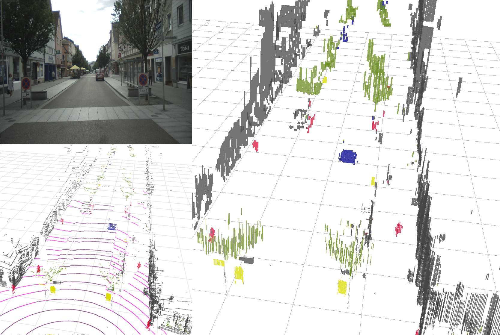
$\bullet$	road
$\bullet$	sidewalk
$\bullet$	person
$\bullet$	rider
$\bullet$	small vehicle
$\bullet$	large vehicle
$\bullet$	two wheeler
$\bullet$	construction
$\bullet$	pole
$\bullet$	traffic sign
$\bullet$	vegetation
$\bullet$	terrain

Figure 1: Example of a multimodal Stixel scene (right) generated based on a camera image (top left) and a semantic point cloud (bottom left). Note that only object Stixels are visualised. The colors correspond to the Cityscapes semantic class color coding [6].

The sensor output usually involves quantities that are derived from raw measurements, such as detailed semantics [5, 22] or object instance knowledge [29, 30]. The different representations provided by the various sensor types are typically fused into an integrated environment model, for example an occupancy grid map [20], to successfully tackle high-level tasks such as object tracking [27] and path planning [3].

Fusing the massive amounts of data provided by multiple different sensors represents a significant challenge in a real-time application. As a way out, mid-level data representations have been proposed that reduce the amount of sensor data but retain the underlying information at the same time. A prime example of such a mid-level representation is the so-called Stixel-World [2, 21, 26, 7, 13] that provides a compact, yet geometrically and semantically consistent model of the observed environment. Thereby a 3D scene is represented by a set of narrow vertical segments, the Stixels, which are described individually by their vertical extent, geometric surface, and semantic label. The Stixel concept was originally applied to stereo camera data, where the segmentation is primarily based on dense disparity data as well as pixel-level semantics obtained from a deep neural network [26, 7, 13].

In this paper, we propose to transfer the Stixel concept into the LiDAR domain to develop a compact and robust mid-level representation for 3D point clouds. Moreover, we extend the Stixel-World to a multimodal representation by incorporating both camera and LiDAR sensor data into the model. The specific combination of the high resolution and semantic detail of RGB imagery with the supreme distance accuracy of LiDAR data in the multimodal Stixel-World results in a very powerful environment representation that outperforms the state-of-the-art (see Fig. 1). Our main contributions can be summarized as follows:

• A compact and robust mid-level representation for semantic LiDAR point clouds based on the Stixel-World

• A multimodal fusion approach integrated into the proposed mid-level representation

• A detailed performance analysis and quantitative evaluation of the proposed methods

Figure 2: Example of a multimodal Stixel scene (right, colors = Cityscapes semantic class [6], each image column is separated into multiple semantic Stixels) and the corresponding LiDAR distance image (center, blue = close, red = far) projected to a cylindrical view. The corresponding camera image is shown on the left.

2 Related Work

The multimodal Stixel approach presented in this paper combines LiDAR distance measurements with the point-wise semantic labeling information obtained from both LiDAR and a monocular camera. We relate our approach to three different categories of existing work: semantic labeling, sensor fusion, and compact mid-level data representations.

First, semantic labeling describes a range of techniques for the measurement-wise (e.g. pixel-wise) assignment of object class or object type. The topic has been well explored within the camera domain [10, 17, 5, 25]. In contrast, semantic labeling for 3D point clouds is a relatively recent topic [23, 24], which has mainly been studied on indoor [1, 8] or stationary outdoor datasets [12]. Within road scenarios, Wu et al. [28] introduced a Fully Convolutional Neural Network (FCN) approach based on the SqueezeNet architecture [14] for semantic labeling of vehicles, pedestrian and cyclists within 3D LiDAR point cloud data. A 2D cylindrical projection of the point cloud (see Fig. 2) is applied, enabling the application of efficient image-based filter kernels. Piewak et al. [22] extend this concept and propose an improved network architecture which is able to perform high-quality semantic labeling of a 3D point cloud based on 13 classes similar to the Cityscapes Benchmark suite [6]. As the multimodal Stixel approach proposed in this paper utilizes semantics from both LiDAR and camera data, we apply the approach of [22] to directly extract the detailed point-wise semantics from LiDAR data. This results in a class representation similar to the camera domain, where we make use of the efficient FCN architecture described by Cordts et al. [5].

Second, different fusion strategies can be applied to the multimodal data of various sensors. Several approaches perform so-called low-level fusion by directly combining the raw data to obtain a joint sensor representation, which is then used for object detection [11] or semantic labeling [19]. A different method commonly used within the autonomous driving context is high-level fusion [20], where the sensor data is processed independently and the results are later combined on a more abstract level. In this paper, we present a novel fusion concept which integrates the sensor data on mid-level, reducing the data volume while minimizing information loss. This representation can further be integrated into a more abstract environment model such as an occupancy grid [20].

Third, the presented multimodal Stixel approach is closely related to other compact mid-level representations in terms of the output data format. In particular, we refer to the Stixel-World obtained from camera imagery, which has successfully been applied with [4, 21, 16] and without [4, 15] the use of stereoscopic depth information. The integration of camera-based semantic labeling information into the Stixel generation process was presented in [26, 5, 13], thereby further improving robustness and promoting the semantic consistency of the result. The Stixel concept has also been adapted to other image-based sensor techniques, for example to a camera-based infrared depth sensor as shown in [18]. Forsberg [9] makes use of a LiDAR scanner to obtain depth information for the Stixel generation process. Similarly to an early idea in [21], the LiDAR point cloud is simply projected into the camera image to replace the original dense disparity information with the sparse LiDAR-based depth measurements. In contrast, we employ a LiDAR-specific sensor model that is particularly tailored to exploit the superior geometric accuracy of the LiDAR sensor over a stereo camera. Finally, we integrate semantics from both LiDAR and camera data into the Stixel generation process to obtain a high-quality, comprehensive mid-level 3D representation of the environment.

3 Method

The proposed Stixel model is inspired by the stereoscopic camera approaches of [21, 26, 7]. After a general definition of the Stixel representation, we describe the transfer of the Stixel model to the LiDAR domain as well as the adapted Stixel generation process.

3.1 Stixel Definition

Stixels are segments which represent sensor data in a compact fashion while retaining the underlying semantic and geometric properties. Generally, the segmentation of an image represents a 2D optimization problem which is challenging to solve in a real-time environment. Instead, Stixels are optimized column-wise, which reduces the optimization task to a 1D problem that can be efficiently solved via dynamic programming [21]. As a result, each column is separated into rectangular stick-like segments S called Stixels. Within the LiDAR domain, we represent the input data as an ordered set of columns of the LiDAR scan, obtained from a cylindrical projection of the 3D measurements onto a 2D grid, as shown in Fig. 2. Each Stixel $\textbf{{s}}_{i}=(b,t,r,l,c)$ is represented by the bottom row index $b$ and the top row index $t$, describing its vertical extent with regard to the vertically ordered measurements $\textbf{{M}}=(\textbf{{m}}_{1},\dots,\textbf{{m}}_{h})$. Additionally, each Stixel has a semantic label $l$, a structural class $c$, and a distance $r$ to the sensor or the ideal ground plane (depending on the structural class $c$). There are three different Stixel structural classes, i.e. support ($\mathcal{G}$) for flat regions such as road surface or sidewalk, object ($\mathcal{O}$) for obstacles such as people or vehicles, and sky ($\mathcal{S}$) for areas without LiDAR measurements, as indicated in Fig. 3.

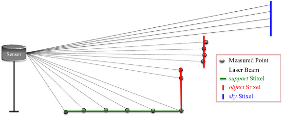
Figure 3: Exemplary Stixel extraction based on a vertical LiDAR scan column.

3.2 Stixel Model

The vertically ordered (bottom to top) set of measurements $\textbf{{M}}=(\textbf{{m}}_{1},\dots,\textbf{{m}}_{h})$ is processed column-wise (see Fig. 2) and contains LiDAR depth measurements $\textbf{{D}}=(\textbf{{d}}_{1},\dots,\textbf{{d}}_{h})$ as well as semantics from the camera $\textbf{{L}}_{cam}=(\textbf{{l}}_{cam_{1}},\dots,\textbf{{l}}_{cam_{h}})$ and the LiDAR $\textbf{{L}}_{lidar}=(\textbf{{l}}_{lidar_{1}},\dots,\textbf{{l}}_{lidar_{h}})$, respectively. The extraction of semantics from the LiDAR is done using the LiLaNet architecture of [22]. The semantic information of the camera is associated to the 3D LiDAR points based on the so-called Autolabeling technique [22], which projects the LiDAR points into the image plane in order to associate the semantics provided by a state-of-the-art image-based FCN to each point.

Based on this definition the posterior distribution $P(\textbf{{S}}|\textbf{{M}})$ of the Stixels S given the measurements M of a column is defined using the likelihood $P(\textbf{{M}}|\textbf{{S}})$ as well as the prior $P(\textbf{{S}})$ as

$$P(\textbf{{S}}|\textbf{{M}})=\frac{P(\textbf{{M}}|\textbf{{S}})\cdot P(\textbf{{S}})}{P(\textbf{{M}})}\text{ .}$$ (1)

Here, the Stixels $\textbf{{S}}=(\textbf{{s}}_{1},\dots,\textbf{{s}}_{n})$ are vertically ordered in accordance with the measurement vector M. Formulating the posterior distribution in the log-domain yields

$$P(\textbf{{S}}|\textbf{{M}})=e^{-E(\textbf{{S}},\textbf{{M}})}\text{ ,}$$ (2)

where $E(\textbf{{S}},\textbf{{M}})$ represents an energy function similar to [7], defined as

$$E(\textbf{{S}},\textbf{{M}})=\Theta(\textbf{{S}},\textbf{{M}})+\Omega(\textbf{{S}})-\log(P(\textbf{{M}}))\text{ .}$$ (3)

Note that $\Theta(\textbf{{S}},\textbf{{M}})$ represents the data likelihood, $\Omega(\textbf{{S}})$ the segmentation prior, and $P(\textbf{{M}})$ a normalizing constant. In contrast to camera-based Stixel applications, as discussed in Section 2, the proposed approach puts forward a LiDAR-specific sensor model to better integrate the accurate LiDAR geometry into the Stixel-World. This will be discussed within the next subsections.

3.2.1 Prior

The prior $\Omega(\textbf{{S}})$ puts constraints on the Stixel model in terms of model complexity and segmentation consistency with

$$\Omega(\textbf{{S}})=\Omega_{mc}(\textbf{{S}})+\Omega_{sc}(\textbf{{S}})\text{ .}$$ (4)

The model complexity term $\Omega_{mc}(\textbf{{S}})$ describes the trade-off between the compactness and the accuracy of the representation. The segmentation consistency $\Omega_{sc}(\textbf{{S}})$ governs hard constraints on the Stixels concerning the relation of Stixels within a column. The formulation of these prior terms does not depend on the LiDAR measurements, similar to existing Stixel approaches in the camera domain. For further details, the reader is referred to [7].

3.2.2 Data Likelihood

The data likelihood represents the matching quality of the measurements M to a given set of Stixels S, considering three different data modalities: LiDAR geometry, LiDAR semantics, and camera semantics:

$$\begin{split}\Theta(\textbf{{S}},\textbf{{M}})=\sum\limits_{\textbf{{s}}_{i}\in\textbf{{S}}}\sum\limits_{\textbf{{m}}_{j}\in\textbf{{M}}^{*}_{i}}&\beta_{geo_{lidar}}\Theta_{geo}(\textbf{{s}}_{i},\textbf{{d}}_{j},\textbf{{d}}_{j-1})\\ &+\beta_{sem_{lidar}}\Theta_{sem_{lidar}}(\textbf{{s}}_{i},\textbf{{l}}_{lidar_{j}})\\ &+\beta_{sem_{cam}}\Theta_{sem_{cam}}(\textbf{{s}}_{i},\textbf{{l}}_{cam_{j}})\text{ .}\end{split}$$ (5)

Here $\textbf{{M}}^{*}_{i}$ represents a subset of the measurements M associated to a specific Stixel $\textbf{{s}}_{i}$. The parameters $\beta_{geo_{lidar}}$, $\beta_{sem_{lidar}}$, and $\beta_{sem_{cam}}$ represent weighting parameters of each modality, which are described within this subsection.

LiDAR Geometry

The LiDAR geometry data likelihood consists of three elements defined as follows:

$$\begin{split}\Theta_{geo}(\textbf{{s}}_{i},\textbf{{d}}_{j},\textbf{{d}}_{j-1})&=\Theta_{dist}(\textbf{{s}}_{i},\textbf{{d}}_{j})+\Theta_{gr}(\textbf{{s}}_{i},\textbf{{d}}_{j},\textbf{{d}}_{j-1})\\ &+\Theta_{sens}(\textbf{{s}}_{i},\textbf{{d}}_{j})\text{ .}\end{split}$$ (6)

First of all, the relation of a LiDAR depth measurement $\textbf{{d}}_{j}$ and the Stixel $\textbf{{s}}_{i}$ is given by the term $\Theta_{dist}(\textbf{{s}}_{i},\textbf{{d}}_{j})$. We represent this data likelihood as a mixture of a normal distribution, encoding the sensor noise based on the variance $\sigma$, and an uniform distribution representing outlier measurements with an outlier rate of $p_{out}$ similar to [7].

In addition to the common depth likelihood definition $\Theta_{dist}(\textbf{{s}}_{i},\textbf{{d}}_{j})$, two additional likelihood terms are defined to take advantage of LiDAR-specific measurement properties: a ground term $\Theta_{gr}(\textbf{{s}}_{i},\textbf{{d}}_{j},\textbf{{d}}_{j-1})$ and a sensor term $\Theta_{sens}(\textbf{{s}}_{i},\textbf{{d}}_{j})$. The ground term assesses the consistency of the data with an assumed ground model, based on the gradient between two measurements

$$\phi(\textbf{{d}}_{j},\textbf{{d}}_{k})=\arctan\left(\frac{\Delta z_{jk}}{d_{ground_{jk}}}\right)=\arctan\left(\frac{z_{k}-z_{j}}{\sqrt{x_{k}^{2}+y_{k}^{2}}-\sqrt{x_{j}^{2}+y_{j}^{2}}}\right)\text{ .}$$ (7)

Note that a geometric LiDAR measurement $\textbf{{d}}_{j}=(r_{j},\alpha_{h_{j}},\alpha_{v_{j}})$ is represented using polar coordinates and consists of a measured distance $r_{j}$, a horizontal angle $\alpha_{h_{j}}$, and a vertical angle $\alpha_{v_{j}}$. Based on these polar coordinates, the Cartesian coordinates $(x_{j},y_{j},z_{j})$ are extracted.

The gradient $\phi$ obtained from the high-quality LiDAR measurements provides structural information of the environment to distinguish between flat surfaces such as ground (low gradient) and obstacles (high gradient). This information is encoded into an object existence probability using a parametrized hyperbolic tangent as

$$P_{ob}(\textbf{{d}}_{j},\textbf{{d}}_{j-1})=\frac{1+\tanh(\beta_{gr,steep}(\phi(\textbf{{d}}_{j},\textbf{{d}}_{j-1})-\beta_{gr,shift}))}{2}\text{ .}$$ (8)

Note that the parameters $\beta_{gr,steep}$ and $\beta_{gr,shift}$ adapt the sensitivity of the gradient model. Subsequently, the data likelihood based on the ground model is defined as

$$\Theta_{gr}(\textbf{{s}}_{i},\textbf{{d}}_{j},\textbf{{d}}_{j-1})=\begin{cases}-\log(1-P_{ob}(\textbf{{d}}_{j},\textbf{{d}}_{j-1}))&\text{if }\phi\text{ is def. and }c_{i}=\mathcal{G}\\ -\log(P_{ob}(\textbf{{d}}_{j},\textbf{{d}}_{j-1}))&\text{if }\phi\text{ is def. and }c_{i}=\mathcal{O}\\ 0&\text{if }\phi\text{ is undef. or }c_{i}=\mathcal{S}\end{cases}\text{ .}$$ (9)

Note that the data likelihood based on the ground model is set to zero when the gradient is undefined, which can be caused by missing reflections of the LiDAR laser light (e.g. if the laser beam is pointing to the sky). However, both the vertical and horizontal angles of the polar coordinate of the so-called invalid measurement are still available.

In case of an invalid measurement, the data likelihood based on both the ground model and the depth matching cannot be processed. For this reason we introduce the sensor term $\Theta_{sens}(\textbf{{s}}_{i},\textbf{{d}}_{j})$ to the likelihood formulation, which is based on the vertical distribution of measurement angles of the LiDAR sensor. We assume that a sky Stixel is more likely to occur at larger vertical angles, which is encoded into a parametrized hyperbolic tangent similar to Eq. 8 as

$$P_{\mathcal{S}}(\alpha_{v_{j}})=\frac{1+\tanh(\beta_{sens,scale}(\alpha_{v_{j}}-\beta_{sens,shift}))}{2}\text{ .}$$ (10)

A similar definition is used with regard to small vertical angles and support Stixels by inverting the vertical angle $P_{\mathcal{G}}(\alpha_{v_{j}})=P_{\mathcal{S}}(-\alpha_{v_{j}})$. Consequently, the sensor term contribution for invalid points is defined by

$$\Theta_{sens}(\textbf{{s}}_{i},\textbf{{d}}_{j})=\begin{cases}-\log(P_{\mathcal{S}}(\alpha_{v_{j}}))&\text{if }\textbf{{d}}_{j}\text{ is invalid and }c_{i}=\mathcal{S}\\ -\log(P_{\mathcal{G}}(\alpha_{v_{j}}))&\text{if }\textbf{{d}}_{j}\text{ is invalid and }c_{i}=\mathcal{G}\\ -\log(1-P_{B}(\alpha_{v_{j}}))&\text{if }\textbf{{d}}_{j}\text{ is invalid and }c_{i}=\mathcal{O}\\ \infty&\text{if }\textbf{{d}}_{j}\text{ is valid and }c_{i}=\mathcal{S}\\ 0&\text{if }\textbf{{d}}_{j}\text{ is valid and }c_{i}\in\{\mathcal{G},\mathcal{O}\}\\ \end{cases}\text{ ,}$$ (11)

with $P_{B}(\alpha_{v_{j}})=P_{\mathcal{S}}(\alpha_{v_{j}})+P_{\mathcal{G}}(\alpha_{v_{j}})$. Note that a hard constraint is inserted to prohibit sky Stixels resulting from valid measurements.

Semantic Information

The semantic information obtained from the LiDAR data is utilized in a similar way as in the Stixel-World of the camera domain. Each semantic measurement $\textbf{{l}}_{lidar_{j}}$ holds a probability estimate $P_{\textbf{{l}}_{lidar_{j}}}(l)$ of each class $l$ conditioned on the input data, which can be obtained from the underlying semantic labeling method. We make use of the LiLaNet architecture of [22] to compute the point-wise LiDAR-based semantic information. The definition of the semantic data likelihood is adapted from [26] and [7] as

$$\Theta_{sem_{lidar}}(\textbf{{s}}_{i},\textbf{{l}}_{lidar_{j}})=-\log(P_{\textbf{{l}}_{lidar_{j}}}(l_{i}))\text{ .}$$ (12)

To obtain high resolution semantic information from the camera image, we make use of the efficient FCN architecture described by Cordts et al. [5]. Fusing this information into the proposed multimodal Stixel approach enables the combination of high resolution camera semantics with geometrically accurate information of the LiDAR. For this purpose we apply the projection technique of [22] to extract the semantic information of the camera by projecting the LiDAR measurements into the semantically labeled image. Each LiDAR measurement then holds additional semantic information from the camera domain $\textbf{{l}}_{cam_{j}}$ which is processed similar to Eq. 12 based on the probability $P_{\textbf{{l}}_{cam_{j}}}(l)$ for each semantic class $l$ with

$$\Theta_{sem_{cam}}(\textbf{{s}}_{i},\textbf{{l}}_{cam_{j}})=-\log(P_{\textbf{{l}}_{cam_{j}}}(l_{i}))\text{ .}$$ (13)

Note that this definition is independent of the LiDAR-based semantics which enables the extraction of different domain specific semantic classes $l$ from camera and LiDAR. Especially the camera-based FCN [5] extracts more semantic classes based on the higher resolution as well as the larger receptive field as the LiDAR-based FCN [22]. Hence, the domain specific strengths of each sensor modality and the differing object appearance within the LiDAR and the camera are combined to increase the semantic consistency of the multimodal Stixel result.

3.3 Stixel Generation

Based on the proposed Stixel model, Stixels are generated by finding the maximum-a-posteriori solution of Eq. 1. This is equal to the minimization of the energy function given in Eq. 3. Note, that the probability of the measurement $P(\textbf{{M}})$ represents a scaling factor which is ignored within the optimization process. To solve this 1D column-wise optimization process, a dynamic programming approach is used similar to the original Stixel formulation (c.f. [21] and [7]).

4 Experiments

To evaluate our proposed multimodal Stixel model, we use the manually annotated dataset of Piewak et al. [22]. The dataset consists of manually annotated semantic LiDAR point clouds recorded from a vehicle in various traffic scenarios, and further includes corresponding image data captured by a front-facing monocular camera. This enables both a semantic evaluation of our proposed method based on the manually annotated semantic LiDAR data and a geometric evaluation based on the LiDAR depth data. Due to the sensor configuration within the dataset, the evaluation is restricted to the area inside the field of view of the camera. We evaluate various performance metrics on a point-wise basis to measure the geometric and semantic consistency as well as the compactness of the model:

1. Outlier Rate

   A relative distance deviation of the original LiDAR depth measurement from the associated Stixel of more than $5\%$ is declared as an outlier. Based on this formulation the outlier rate is defined as the ratio of the number of outliers to the number of total LiDAR points.

2. Intersection over Union (IoU)

   Based on the manually annotated semantic ground truth, an IoU of the Stixels to the ground truth LiDAR points can be calculated similar to [6].

3. Compression Rate

   The data compression rate $\theta$ defines the ratio between the number of stixels $n_{stixels}$ and number of original LiDAR points $n_{points}$ via

   $$\theta=1-\frac{n_{stixels}}{n_{points}}\text{ .}$$ (14)

Figure 4: Impact of considering the semantic information within the multimodal Stixel model with a constant LiDAR geometry weight ($\beta_{geo_{lidar}}=1$). left: Adaption of the LiDAR semantic weight $\beta_{sem_{lidar}}$ based on a deactivated camera semantics ($\beta_{sem_{cam}}=0$). right: Adaption of the camera semantic weight $\beta_{sem_{cam}}$ based on a LiDAR semantic weight $\beta_{sem_{lidar}}=1$

The quantitative results are illustrated in Fig. 4. First, the impact of the LiDAR semantic weight $\beta_{sem_{lidar}}$ is evaluated while the LiDAR geometry weight is set to $\beta_{geo_{lidar}}=1$ and the camera semantics is deactivated ($\beta_{sem_{cam}}=0)$. We observe that the semantic consistency is constantly increasing with an increase of the LiDAR semantic weight. At the same time, the compression rate increases as well as the outlier rate. Putting too much focus on the semantic input thus reduces the number of individual Stixels and yields a model purely tuned to the LiDAR semantics. In turn, consistency with the underlying geometry decreases.

Considering the multimodality in our model by activating the camera semantics, the compression rate as well as the outlier rate slightly decreases. The semantic consistency further improves until the weighting of the camera semantics $\beta_{sem_{cam}}$ reaches the weighting of the LiDAR semantics $\beta_{sem_{lidar}}$. However, the camera semantics on its own reaches a lower IoU after the transfer to the LiDAR domain (see Table 1). This demonstrates the potential of our novel multimodal Stixel approach, which creates a compact, geometrically and semantically consistent mid-level representation by combining the advantages of different sensor domains to reach a higher accuracy than each modality on its own. Our proposed method of equally weighting the different modalities represents the best combination with regard to the semantic consistency as well as a good compromise concerning the outlier rate and the compression rate. This setup outperforms the original Stixel-World based on a stereoscopic camera regarding the geometric and the semantic consistency of the data representation (see Table 1).

Table 1: Comparison of the original Stixel World (based on a stereoscopic camera), the different independent Stixel optimization modalities, and the combined multimodal representation.

	Stereo Camera [7]	LiDAR Depth only	LiDAR Semantics only	Camera Semantics only	Multi-Modality
Outlier Rate in %	6.7	0.62	28.8	35.3	0.95
IoU in %	66.5	61.8	70.0	60.8	70.6
Compression Rate in %	_	54.0	81.2	85.3	58.3

5 Conclusion

In this paper, we presented the multimodal Stixel-World, a Stixel-based environment representation to directly leverage both camera and LiDAR sensor data. Our design goal is to jointly represent accurate geometric and semantic information based on a multi-sensor system within a compact and efficient environment model. To this end we introduce a LiDAR-specific sensor model that exploits the geometric accuracy of LiDAR sensors as well as a mid-level fusion technique to combine valuable semantic information from both camera and LiDAR. In our experiments we demonstrated the benefits of our multimodal Stixel-World over unimodal representations in terms of representation and compression quality by outperforming the original Stixel-World based on a stereoscopic camera. Moreover, our presented multimodal Stixel approach can easily be extended to other sensor modalities as long as they can be projected into a common structured data format.

References

- [1] Armeni, I., Sax, S., Zamir, A.R., et al.: Joint 2D-3D-Semantic Data for Indoor Scene Understanding. In: arXiv preprint:1702.01105 (2017)
- [2] Badino, H., Franke, U., Pfeiffer, D.: The Stixel World - A Compact Medium Level Representation of the 3D-World. In: Denzler, J., Notni, G., Süße, H. (eds.) Pattern Recognition. pp. 51–60. Springer, Berlin (2009)
- [3] Bai, H., Cai, S., Ye, N., et al.: Intention-aware online POMDP planning for autonomous driving in a crowd. In: International Conference on Robotics and Automation (ICRA) (2015)
- [4] Benenson, R., Mathias, M., Timofte, R., et al.: Fast Stixel Computation for Fast Pedestrian Detection. In: European Conference on Computer Vision (ECCV) Workshop (2012)
- [5] Cordts, M.: Understanding Cityscapes: Efficient Urban Semantic Scene Understanding. Phd thesis, Technische Universität Darmstadt (2017)
- [6] Cordts, M., Omran, M., Ramos, S., et al.: The Cityscapes Dataset for Semantic Urban Scene Understanding. In: Conference on Computer Vision and Pattern Recognition (CVPR) (2016)
- [7] Cordts, M., Rehfeld, T., Schneider, L., et al.: The Stixel World: A medium-level representation of traffic scenes. Image and Vision Computing 68, 40–52 (2017)
- [8] Dai, A., Chang, A.X., Savva, M., et al.: ScanNet: Richly-Annotated 3D Reconstructions of Indoor Scenes. In: Conference on Computer Vision and Pattern Recognition (CVPR) (2017)
- [9] Forsberg, O.: Semantic Stixels fusing LIDAR for Scene Perception Semantic Stixels fusing LIDAR for Scene Perception (2018)
- [10] Garcia-Garcia, A., Orts-Escolano, S., Oprea, S., et al.: A Review on Deep Learning Techniques Applied to Semantic Segmentation. In: arXiv preprint: 1704.06857 (2017)
- [11] Gupta, S., Girshick, R.B., Arbeláez, P.A., et al.: Learning Rich Features from RGB-D Images for Object Detection and Segmentation. In: European Conference on Computer Vision (ECCV) (2014)
- [12] Hackel, T., Savinov, N., Ladicky, L., et al.: SEMANTIC3D.NET: A new large-scale Point Cloud Classification Benchmark. Annals of Photogrammetry, Remote Sensing and Spatial Information Sciences (ISPRS) IV-1/W1, 91–98 (2017)
- [13] Hernandez-Juarez, D., Schneider, L., Espinosa, A., et al.: Slanted Stixels: Representing San Francisco’s Steepest Streets. In: British Machine Vision Conference (BMVC) (2017)
- [14] Iandola, F.N., Han, S., Moskewicz, M.W., et al.: SqueezeNet: AlexNet-level accuracy with 50x fewer parameters and <0.5MB model size. In: arXiv preprint: 1602.07360 (2016)
- [15] Levi, D., Garnett, N., Fetaya, E.: StixelNet: A Deep Convolutional Network for Obstacle Detection and Road Segmentation. In: British Machine Vision Conference (BMVC) (2015)
- [16] Liu, M.Y., Lin, S., Ramalingam, S., et al.: Layered Interpretation of Street View Images. In: Robotics: Science and Systems. Robotics: Science and Systems Foundation (2015)
- [17] Long, J., Shelhamer, E., Darrell, T.: Fully Convolutional Networks for Semantic Segmentation ppt. In: Conference on Computer Vision and Pattern Recognition (CVPR) (2015)
- [18] Martinez, M., Roitberg, A., Koester, D., et al.: Using Technology Developed for Autonomous Cars to Help Navigate Blind People. In: Conference on Computer Vision Workshops (ICCVW) (2017)
- [19] Muller, A.C., Behnke, S.: Learning depth-sensitive conditional random fields for semantic segmentation of RGB-D images. In: Conference on Robotics and Automation (ICRA) (2014)
- [20] Nuss, D., Reuter, S., Thom, M., et al.: A Random Finite Set Approach for Dynamic Occupancy Grid Maps with Real-Time Application. In: arXiv preprint: 1605.02406 (2016)
- [21] Pfeiffer, D.: The Stixel World - A Compact Medium-level Representation for Efficiently Modeling Dynamic Three-dimensional Environments. Phd thesis, Humboldt-Universität Berlin (2012)
- [22] Piewak, F., Pinggera, P., Schäfer, M., et al.: Boosting LiDAR-based Semantic Labeling by Cross-Modal Training Data Generation. In: arXiv preprint: 1804.09915 (2018)
- [23] Qi, C.R., Yi, L., Su, H., et al.: PointNet++: Deep Hierarchical Feature Learning on Point Sets in a Metric Space. In: Advances in Neural Information Processing Systems (NIPS) (2017)
- [24] Riegler, G., Ulusoy, A.O., Geiger, A.: OctNet: Learning Deep 3D Representations at High Resolutions. In: Computer Vision and Pattern Recognition (CVPR) (2017)
- [25] Sankaranarayanan, S., Balaji, Y., Jain, A., et al.: Learning from Synthetic Data: Addressing Domain Shift for Semantic Segmentation. In: arXiv preprint:1711.06969 (2017)
- [26] Schneider, L., Cordts, M., Rehfeld, T., et al.: Semantic Stixels: Depth is not enough. In: Intelligent Vehicles Symposium (IV) (2016)
- [27] Vu, T.d., Burlet, J., Aycard, O., et al.: Grid-based localization and local mapping with moving object detection and tracking Grid-based Localization and Local Mapping with Moving Object Detection and Tracking. Journal Information Fusion 12(1), 58–69 (2011)
- [28] Wu, B., Wan, A., Yue, X., et al.: SqueezeSeg: Convolutional Neural Nets with Recurrent CRF for Real-Time Road-Object Segmentation from 3D LiDAR Point Cloud. In: arXiv preprint: 1710.07368 (2017)
- [29] Yang, F., Choi, W., Lin, Y.: Exploit All the Layers: Fast and Accurate CNN Object Detector with Scale Dependent Pooling and Cascaded Rejection Classifiers. In: Conference on Computer Vision and Pattern Recognition (CVPR) (2016)
- [30] Zhou, Y., Tuzel, O.: VoxelNet: End-to-End Learning for Point Cloud Based 3D Object Detection. In: arXiv preprint: 1711.06396 (2017)