Symmetry-adapted decomposition of tensor operators and the visualization of coupled spin systems

Abstract

We study the representation and visualization of finite-dimensional quantum systems. In a generalized Wigner representation, multi-spin operators can be decomposed into a symmetry-adapted tensor basis and they are mapped to multiple spherical plots that are each assembled from linear combinations of spherical harmonics. We apply two different approaches based on explicit projection operators and coefficients of fractional parentage in order to obtain this basis for up to six spins $1/2$ (qubits), for which various examples are presented. An extension to two coupled spins with arbitrary spin numbers (qudits) is provided, also highlighting a quantum system of a spin $1/2$ coupled to a spin $1$ (qutrit).

smalltableaux,centertableaux

I Introduction

Quantum systems exhibit an intricate structure and numerous methods have been established for the visualization of their quantum state. A two-level quantum system, such as a single spin $1/2$ (qubit), can always be faithfully represented by a three-dimensional vector (Bloch vector), as shown in the seminal work of Feynman et al.Feynman, Vernon, and Hellwarth (1957) Applications of the Bloch vector are frequently found in the field of quantum physics, in particular in magnetic resonance imaging,Bernstein, King, and Zhou (2004); Ernst, Bodenhausen, and Wokaun (1987) spectroscopy,Ernst, Bodenhausen, and Wokaun (1987) and quantum optics.Schleich (2001) However, for systems consisting of coupled spins, standard Bloch vectors can only partially represent the density matrix, whereas important terms, such as multiple-quantum coherenceErnst, Bodenhausen, and Wokaun (1987) or spin alignment,Ernst, Bodenhausen, and Wokaun (1987) are not captured. In this case, the complete density operator can be visualized by bar charts, in which the real and imaginary parts of each element of the density matrix is represented a vertical bar, an approach which is commonly used to graphically display the experimental results of quantum state tomography.Nielsen and Chuang (2000) Alternatively, energy-level diagrams can can be illustrate populations by circles on energy levels and coherences by lines between energy levels.Sørensen et al. (1983) Density operators can also be visualized by non-classical vector representations based on single-transition operators.Ernst, Bodenhausen, and Wokaun (1987); Donne and Gorenstein (1997); Freeman (1997) However, these techniques are inconvenient for larger spin systems and often do not provide an intuitive view of the spin dynamics.

Phase space representations,Schleich (2001); Curtright, Fairlie, and Zachos (2014); Zachos, Fairlie, and Curtright (2005); Schroeck Jr. (2013) in particular Wigner functions,Wigner (1932); Schleich (2001); Curtright, Fairlie, and Zachos (2014) which originally arise in the description of the infinite-dimensional quantum state of light,Smithey et al. (1993a, b, c); Leonhardt (1997); Paris and Rehacek (2004) provide a powerful alternative approach for the characterization and visualization of finite-dimensional quantum systems. One valuable class for the representation of finite-dimensional systems are discrete Wigner functions Wooters (1987); Leonhardt (1996); Miquel, Paz, and Saraceno (2002); Miquel et al. (2002); Gibbons, Hoffman, and Wootters (2004); Ferrie and Emerson (2009) but we will focus on continuous representations, which naturally reflect the inherent rotational symmetries of spins. General criteria for defining continuous Wigner functions for finite-dimensional quantum systems had been established in the work by StratonovichStratonovich (1956) and the case of single-spin systems has been studied in the literature.Agarwal (1981); Várrily and Garcia-Bondía (1989); Brif and Mann (1999, 1997); Heiss and Weigert (2000); Klimov (2002); Klimov and Espinoza (2005, 2002) Extensions to multiple spins have been considered in Ref. Schleich, 2001; Dowling, Agarwal, and Schleich, 1994; Jessen et al., 2001; Philp and Kuchel, 2005; Harland et al., 2012, but a general strategy for multiple coupled spins was still missing.Philp and Kuchel (2005); Harland et al. (2012) Recently, Garon et al.Garon, Zeier, and Glaser (2015) identified such a general strategy. Subsequently, further approaches to phase-space representations have been developed,Tilma et al. (2016); Koczor, Zeier, and Glaser (2016); Rundle et al. (2017a, b); Koczor, Zeier, and Glaser (2017, 2018) while rotated parity operatorsHeiss and Weigert (2000); Tilma et al. (2016); Rundle et al. (2017a, b); Koczor, Zeier, and Glaser (2017, 2018) and tomographic techniquesRundle et al. (2017a); Leiner, Zeier, and Glaser (2017); Koczor, Zeier, and Glaser (2017); Leiner and Glaser (2018) became further focal points.

We build in this work on the general Wigner representation for multiple coupled spins introduced in Ref. Garon, Zeier, and Glaser, 2015. This Wigner representation is denoted as DROPS representation (discrete representation of operators for spin systems). It is based on mapping operators to a finite set of spherical plots, which are each assembled from linear combinations of spherical harmonicsJackson (1999) and which are denoted as droplets or droplet functions.Garon, Zeier, and Glaser (2015) These characteristic droplets preserve crucial symmetries of the quantum system. One particular version of this representation relies on a specific choice of a tensor-operator basis, the so-called LISA basis,Garon, Zeier, and Glaser (2015) which characterizes tensors according to their linearity, their set of involved spins, their permutation symmetries with respect to spin permutations, and their rotation symmetries under rotations that operate uniformly on each spin. These symmetry-adapted tensors can be constructed using explicit projection operators given as elements of the group ring of the symmetric group.James (1978); James and Kerber (1981); Ceccherini-Silberstein, Scarabotti, and Tolli (2010); Boerner (1967); Hamermesh (1962); Sagan (2001); Tung (1985); Garon, Zeier, and Glaser (2015) We apply this approach to a larger number of coupled spins $1/2$ (qubits) and also to two-spin systems with arbitrary spin numbers (qudits). In addition, we implement a second, alternative computational methodology that relies on so-called coefficients of fractional parentage (CFP)Racah (1965); Elliott and Lane (1957); Kaplan (1975); Silver (1976); Chisholm (1976); Kramer, John, and Schenzle (1981); Jahn and van Wieringen (1951) in order to obtain the symmetry-adapted LISA basis.

Our contribution can also be put into a general context of symmetry-adapted decompositions of tensor operators. Symmetry-adapted (tensor) bases have a very long tradition in physics. Important mathematical contributions were made by WeylWeyl (1927, 1931, 1950, 1953) and Wigner,Wigner (1931, 1959) even though the corresponding group theory was (at least in the beginning) not universally embraced in the physics community (see p. 10-11 in Ref. Condon and Shortley, 1935). Building on Ref. Condon and Shortley, 1935, RacahRacah (1941, 1942, 1943, 1949, 1965); Fano and Racah (1959) developed tensor-operator methods for the analysis of electron spectra. These tensor methods have been widely studiedEdmonds (1960); Griffith (2006); Judd (1998); Silver (1976) and initiated an active exchange between group theory and physics.Weyl (1950); Wigner (1959); Hamermesh (1962); Boerner (1967); Miller (1972); Tung (1985); Ludwig and Falter (1996) Moreover, tensor operators (as well as coefficients of fractional parentage) play an important role in applications to atomic and nuclear structure for which an expansive literature exsists.Elliott and Lane (1957); Slater (1960); de-Shalit and Talmi (1963); Pauncz (1967); Wybourne (1970); Kaplan (1975); Chisholm (1976); Elliott and Dawber (1979); Condon and Odabaşi (1980); Rudzikas (1997); Chaichian and Hagedorn (1998); Rowe and Wood (2010) In this context, we also mention the work of Listerud et al.Listerud (1987); Listerud, Glaser, and Drobny (1993) which partly motivated the approach taken in Ref. Garon, Zeier, and Glaser, 2015 and this work.

This paper is structured as follows. In Sec. II, we introduce the symmetry-adapted tensor basis and its mapping to Wigner functions. An overview of the construction process of this tensor basis using either explicit projection operators or fractional parentage coefficients is presented in Sec. III. In Sec. IV, the tensor-operator basis is illustrated for up to six coupled spins $1/2$ by examples and applications from quantum information and nuclear magnetic resonance spectroscopy. Coupled two-spin systems with arbitrary spin numbers are treated in Sec. V. The explicit construction of the tensor-operator basis is detailed in Sec. VI. Before we conclude, challenges related to the construction method that relies on explicit projection operators are discussed in Sec. VII. Additional illustrative examples for spins $1/2$ are presented in Appendix A and Appendix B lists the employed values of the fractional parentage coefficients.

II Symmetry-adapted decomposition and visualization of operators of coupled spin systems

We summarize the approach of Ref. Garon, Zeier, and Glaser, 2015 (see also Refs. Leiner, Zeier, and Glaser, 2017; Leiner and Glaser, 2018) to visualize operators of coupled spin systems using multiple droplet functions which are chosen according to a suitable symmetry-adapted decomposition of the tensor-operator space. This allows us to also fix the setting and notation for this work. The general idea relies on mappingSilver (1976); Chaichian and Hagedorn (1998) components $T_{jm}^{(\ell)}$ of irreducible tensor operatorsWigner (1931, 1959); Racah (1942); Biedenharn and Louck (1981) $T_{j}^{(\ell)}$ to spherical harmonicsJackson (1999); Note (1) $Y_{jm}=Y_{jm}(\theta,\phi)$. An arbitrary operator $A$ in a coupled spin system can be expanded into linear combinations

$$A=\sum_{\ell}A^{(\ell)}=\sum_{\ell}\sum_{j\in\mathcal{J}(\ell)}\sum_{m=-j}^{j}c_{jm}^{(\ell)}T_{jm}^{(\ell)}$$ (1)

of tensor components $T_{jm}^{(\ell)}$ according to rank $j$ and order $m$ with $-j\leq m\leq j$ and suitably chosen labels (or quantum numbers) $\ell$, such that the set $\mathcal{J}(\ell)$ of ranks $j$ occurring for each label $\ell$ does not contain any rank twice. Depending on the chosen labels, certain properties and symmetries of the spin system are emphasized. Each component $A^{(\ell)}$ is now bijectively mapped to a droplet function $f^{(\ell)}=f^{(\ell)}(\theta,\phi)$, which can be decomposed into

$$f^{(\ell)}=\sum_{j\in\mathcal{J}(\ell)}\sum_{m=-j}^{j}c_{jm}^{(\ell)}Y_{jm},$$ (2)

where the coefficients $c_{jm}^{(\ell)}$ in Eqs. (1) and (2) are identical. This approach enables us to represent each operator component $A^{(\ell)}$ by a droplet function $f^{(\ell)}$, which is given by its expansion into spherical harmonics, refer to the example on the r.h.s of Table 1. The droplet functions $f^{(\ell)}$ are denoted as droplets and the set of all droplets form the full DROPS representation of an arbitrary operator $A$.

Table 1: Overview of how irreducible tensor operators $T_{j}^{(\ell)}$ with components $T_{jm}^{(\ell)}$ are partitioned in the LISA basis according to their label $\ell$ and rank $j$ for the prototypical case of six spins $1/2$ (left). For a generic operator with randomly chosen complex matrix elements, the droplet functions $f^{(\ell)}$ are illustrated separately for each label $\ell$ (right). For all droplet functions, the maximum radii are normalized to one for better visibility. Each label $\ell$ consists of a number of sublabels: the cardinality $g$ of the set of involved spins (i.e. the $g$-linearity) and the explicit set $G$, the symmetry type given by a standard Young tableau $\tau_{i}^{[g]}$ of size $g$ and, possibly, an ad hoc label given by a roman numeral. Ad hoc sublabels are necessary for $g=6$ as otherwise one could not distinguish, for instance, between the doubly occurring rank $2$ (in bold) for the symmetry type $\tau_{7}^{[6]}$. The structure of the partitioning is illustrated on the right for the zero-linear term (Id) and selected linear, bilinear, trilinear, and 6-linear components. Plots for all possible droplet functions are shown in Table 2 for a system consisting of four spins and in Figs. LABEL:fig:6spin_1d2 and LABEL:fig:6spin_1d2_B for six spins.

The task to find suitable labels $\ell$ that allow for a complete decomposition of the tensor-operator space according to Eq. (1) has been widely studiedJudd et al. (1974); Sharp (1975); Iachello and Levine (1995); Rowe and Wood (2010) and is related to the search for a complete set of mutually commuting operators or good quantum numbers.Merzbacher (1998) Different possibilities have been discussed in Ref. Garon, Zeier, and Glaser, 2015, but here we will focus on the LISA basis,Garon, Zeier, and Glaser (2015) whose labeling scheme is outlined in Tab. 1. First, tensor basis operators are subdivided with respect to the cardinality $g\in\{0,1,\dots,N\}$ of the set of involved spins (i.e. their $g$-linearity), where $N$ denotes the total number of spins. Second, tensor operators with identical $g$-linearity are further partitioned according to the explicit set $G\in\binom{\{1,2,\dots,N\}}{g}$ of involved spins, where $\binom{\{1,2,\dots,N\}}{g}$ denotes the set of all subsets of $\{1,2,\dots,N\}$ with cardinality $\lvert G\rvert=g$. For example for $g=2$ and $N=4$, we obtain $G\in\{\{1,\!2\},\{1,\!3\},\{1,\!4\},\{2,\!3\},\{2,\!4\},\{3,\!4\}\}$. Third, we further partition with respect to the symmetry type given by a standard Young tableauBoerner (1967); Hamermesh (1962); Pauncz (1995); Sagan (2001) $\tau_{i}^{[g]}$ of size $g$ (and with at most $(2J{+}1)^{2}{-}1=4J(J{+}1)$ rows, depending on the spin number $J$), which results in a decomposition according to symmetries under permutations of the set $G$. For reference, all potentially occurring symmetry types $\tau_{i}^{[g]}$ for $g\in\{1,2,3,4,5,6\}$ are uniquely enumerated and specified according to their index $i$ in Tables 2 and LABEL:tab:tableaux. For $g=3$ and $G=\{1,\!2,\!3\}$ we have the symmetry types

$$\tau_{1}^{[3]}=\ytableaushort{123}\,,\;\tau_{2}^{[3]}=\ytableaushort{12,3}\,,\;\tau_{3}^{[3]}=\ytableaushort{13,2}\,,\;\tau_{4}^{[3]}=\ytableaushort{1,2,3},$$ (3)

and equivalent symmetry types arise for all the other sets $G\in\binom{\{1,2,\dots,N\}}{3}$ of involved spins with $\lvert G\rvert=g=3$. Fourth, an ad hoc sublabel $\mathcal{A}$ given by a roman numeral is used to distinguish between cases if the same rank occurs more than one.Feenberg and Phillips (1937); Jahn and van Wieringen (1951) For $g=6$ and the symmetry type $\tau_{7}^{[6]}$, the rank of $j=2$ (as shown in bold on the l.h.s. of Table 1) would occur twice if these cases would have not been distinguished by the ad hoc sublabels $I$ and $II$. In summary, our labeling scheme for the LISA basis is given by $\ell:=(G,\tau^{[g]},\mathcal{A}$). We often suppress redundant sublabels. As discussed in more detail in Sec. V, for systems containing spins with spin numbers larger than $1/2$, the decomposition structure is considerably simplified by additional parent sublabels $\mathcal{P}$.

III Summary of the computational techniques used to construct the LISA basis

In this section, we provide an overview how to explicitly construct the LISA basis, which has been introduced in Sec. II. We focus on spin systems where each spin has the same spin number $J\in\{1/2,1,3/2,\dots\}$. The LISA basis is a symmetry-adapted basis according to symmetries under simultaneous $\mathrm{SU}(2)$ rotations of spins as well as under spin permutations. As discussed in Sec. II, these symmetries of a tensor operator $T_{jm}^{(G,\tau^{[g]},\mathcal{A})}$ are specified by the rank $j$ and order $m$ as well as the symmetry type $\tau^{[g]}$. We start by discussing the simple cases of zero and one spins and explain how to use the Clebsch-Gordan decompositionWigner (1959); Biedenharn and Louck (1981); Zare (1988); Beringer, J. et al. (2012) (Particle Data Group) to symmetrize tensors according to $\mathrm{SU}(2)$ symmetries when a new spin is added to a spin system. This is the first step of the iterative construction, which is schematically illustrated in Fig. 1. Depending on the spin system, in the second step two alternative methods (denoted A and B) are used for the symmetrizing with respect to spin permutations. Method A relies on explicit projection operatorsBoerner (1967); Hamermesh (1962); Sanctuary and Temme (1985); Tung (1985); Sagan (2001) and symmetrizes all $g$-linear tensors in one step. Method B uses a basis change according to fractional parentage coefficientsRacah (1965); Elliott and Lane (1957); Kaplan (1975); Silver (1976); Chisholm (1976); Kramer, John, and Schenzle (1981); Jahn and van Wieringen (1951) (CFP) and iteratively symmetrizes $g$-linear tensors with respect to spin permutations, which in the previous iteration have already been partially symmetrized with respect to the first $g{-}1$ spins. We close this section by discussing sign conventions and how to embed $g$-linear tensors into larger spin systems. Further details are deferred to Sec. VI.

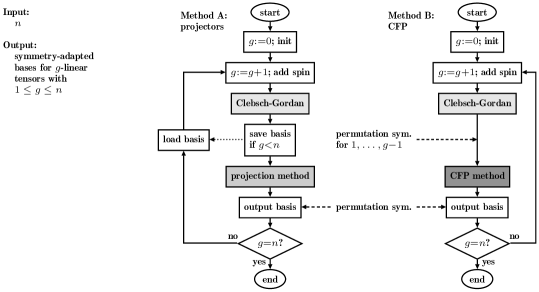
Figure 1: Flow charts for methods A and B used to iteratively construct $g$-linear tensors for $g\in\{1,\ldots,n\}$. Both methods rely first on a Clebsch-Gordan decomposition to symmetrize tensors according to $\mathrm{SU}(2)$ symmetries after adding an additional spin. In a second step, Method A applies projection operators to symmetrize the tensors with respect to permutations. Method B uses a basis change according to fractional parentage coefficients (CFP), in order to completely permutation symmetrize the tensors, which already have been partially symmetrized with respect to the first $g{-}1$ spins in the previous iteration.

For zero-linear tensors (i.e. $g=0$), we have the tensor operator $T^{[0]}_{0}$ with the single component $T^{[0]}_{00}$. We use the notation $T^{[g]}_{j}$ for general $g$-linear tensors of rank $j$, but we will often drop the index $[g]$. For the spin number $J=1/2$, we in particular obtainErnst, Bodenhausen, and Wokaun (1987)

$$T^{[0]}_{00}=T_{00}=\frac{1}{\sqrt{2}}\begin{pmatrix}1&0\\ 0&1\end{pmatrix}.$$ (4)

For linear tensors and spin number $J=1/2$ (i.e. qubits), we have the three componentsErnst, Bodenhausen, and Wokaun (1987)

$$T^{[1]}_{1,-1}=T_{1,-1}=\begin{pmatrix}0&0\\ 1&0\end{pmatrix},\;T^{[1]}_{10}=T_{10}=\frac{1}{\sqrt{2}}\begin{pmatrix}1&0\\ 0&-1\end{pmatrix},\;T^{[1]}_{11}=T_{11}=\begin{pmatrix}0&-1\\ 0&0\end{pmatrix}$$ (5)

of the tensor operator $T^{[1]}_{1}$. For a general spin number $J$ (i.e. qudits), all tensor operators ${}^{J}T^{[1]}_{j}={}^{J}T_{j}$ with $j\in\{1,\ldots,2J\}$ are present. Their tensor operator components ${}^{J}T_{jm}$ with $m\in\{-j,\ldots,j\}$ are given as (see, e.g., Refs. Fano, 1953; Biedenharn and Louck, 1981; Brif and Mann, 1999)

$$\left[{}^{J}T_{jm}\right]_{m_{1}m_{2}}=\sqrt{\tfrac{2j{+}1}{2J{+}1}}C^{Jm_{1}}_{Jm_{2}jm}=(-1)^{J-m_{2}}C^{jm}_{Jm_{1}J,-m_{2}}$$ (6)

in terms of Clebsch-Gordan coefficientsWigner (1959); Biedenharn and Louck (1981); Zare (1988); Beringer, J. et al. (2012) (Particle Data Group) where $m_{1},m_{2}\in\{J,\ldots,-J\}$. Clebsch-Gordan coefficients are the expansion coefficients of a (coupled) total angular momentum eigenbasis in an (uncoupled) tensor product basis. We note that the Clebsch-Gordan coefficients in Eq. (6) describe the (tensor-product) combination of pure states into a density matrix $\lvert\psi_{1}\rangle\langle\psi_{2}\rvert=\lvert\psi_{1}\rangle\otimes\langle\psi_{2}\rvert$ of a single spin. Tables for the Clebsch-Gordan coefficients can be found in literatureBeringer, J. et al. (2012) (Particle Data Group) and there also exist several methods for their computation including recursion relations and explicit formulas.Wigner (1959); Biedenharn and Louck (1981); Messiah (1962); Landau and Lifshitz (1977)

After adding an additional spin, a basis change according to Clebsch-Gordan coefficientsWigner (1959); Biedenharn and Louck (1981); Zare (1988); Beringer, J. et al. (2012) (Particle Data Group) is applied in both methods A and B (see Fig. 1). The Clebsch-Gordon decompositionWigner (1959); Biedenharn and Louck (1981); Zare (1988); Beringer, J. et al. (2012) (Particle Data Group) describes how a tensor product of two irreducible representations is expanded into a direct sum of irreducible representations: the tensor product of two tensor operators $T_{j_{1}}$ and $T_{j_{2}}$ with ranks $j_{1}$ and $j_{2}$ are split up according to

$$T_{j_{1}}\otimes T_{j_{2}}=\bigoplus_{j=|j_{l}-j_{2}|}^{j_{l}+j_{2}}T_{j}.$$ (7)

The $2j{+}1$ tensor components $T_{jm}$ with $m\in\{-j,\dots,j\}$ of each tensor $T_{j}$ on the r.h.s. of Eq. (7) are given by

$$T_{jm}=\sum_{j=|j_{l}-j_{2}|}^{j_{l}+j_{2}}\sum_{m=m_{1}+m_{2}}C^{jm}_{j_{1}m_{1}j_{2}m_{2}}\,T_{j_{1}m_{1}}\otimes T_{j_{2}m_{2}}$$ (8)

via the Clebsch-Gordon coefficientsWigner (1959); Biedenharn and Louck (1981); Zare (1988); Beringer, J. et al. (2012) (Particle Data Group) $C_{j_{1}m_{1}j_{2}m_{2}}^{jm}$. Here, the Clebsch-Gordan coefficients in Eq. (8) describe how tensor operators for $g{-}1$ spins are combined with the ones for a single spin into tensor operators for $g$ spins. In the case of spins $1/2$, tensor operators $T_{j_{1}}$ obtained from the last iteration are combined with the tensor operator $T_{j_{2}}=T_{1}$ (see Eqs. (7) and (8)). For higher spin numbers $J$, the tensor operator $T_{j_{2}}$ is substituted by the direct sum $\oplus_{q=1}^{2J}T_{q}$. More concretely, a $(g{-}1)$-spin system is joined with a single spin $J$, which results in a $g$-spin system such that a $(g{-}1)$-linear tensor $T_{j_{1}}$ generates a set of $g$-linear tensors $T_{j}$:

$$T_{j_{1}}\otimes\left(\bigoplus_{q=1}^{2J}\,T_{q}\right)=\bigoplus_{q=1}^{2J}\bigoplus_{j=|j_{1}-q|}^{j_{1}+q}T_{j}.$$ (9)

The corresponding $g$-linear tensor components $T_{jm}$ with $m=m_{1}+k$ and $k\in\{-q,\ldots,q\}$ are determined from the tensor components $T_{j_{1}m_{1}}$ and $T_{qk}$ via Clebsch-Gordan coefficients as detailed in Eq. (8). After the Clebsch-Gordan basis change, either method A or B is used for the symmetrization with respect to spin permutations. Details are treated in Sec. VI.

The discussed $g$-linear tensor operator components $T_{jm}$ of a rank $j$ and degree $m$ are only defined up to a phase. We employ the Condon-Shortley phase conventionCondon and Shortley (1935); Wigner (1959); Biedenharn and Louck (1981) $T_{jm}=(-1)^{m}T_{jm}^{\dagger}$ that restricts the phase freedom to a freedom of choosing an arbitrary sign for each rank $j$. In order to uniquely specify the tensor operators, we fix these sign factors as detailed in Sec. VI.3. Finally, the $g$-linear tensor operators are embedded into various $N$-spin systems via $N{-}g$ tensor products with suitably positioned tensor operators ${}^{J}T^{\emptyset}_{00}$, which are proportional to identity matrices. For each $N$-spin system, the $g$-linear tensor operators are embedded according to the $\binom{N}{g}$ available subsets $G\in\binom{\{1,\ldots,N\}}{g}$. For example, we denote by $T^{\emptyset}_{00}$ the embedded variant of the zero-linear tensor operator component $T^{[0]}_{00}$ and the linear tensor operators $T^{[1]}_{j}$ result in the embedded tensor operator $T^{G}_{j}$ for each single-element set $G\in\{\{1\},\{2\},\dots,\{N\}\}$ of involved spins.

IV Examples and applications for multiple spins $1/2$

In this section, we present examples and applications for multiple spins $1/2$ and thereby illustrate and motivate our visualization approach. We focus on four and more spins $1/2$, as examples for the case of up to three spins $1/2$ have already been discussed in Ref. Garon, Zeier, and Glaser, 2015. Building on the general outline given in Sec. II, we start by discussing the labels and their structure for four spins $1/2$.

Table 2: Decomposition structure of four coupled spins $1/2$ into linearity $g$, tableau $\tau_{i}^{[g]}$ (or simply $\tau_{i}$ for fixed $g$), and ranks $j$ (left). For each subsystem $G\in\binom{\{1,..,4\}}{2}$, the bilinear tensors corresponding to different tableaux are assembled in a single droplet function and hence the label $\ell$ of bilinear droplets does not contain a sublabel corresponding to a specific tableau $\tau_{i}^{[4]}$. The permutation symmetry corresponding to tableau $\tau_{10}^{[4]}$ does not appear in the four-spin-$1/2$ system, i.e. no rank $j$ exists, which is indicated by “-” at the bottom of the last column. On the right side, all droplet functions visualize together a complex random matrix. For each linearity $g$ multiple subsystems $G\in\binom{\{1,..,4\}}{g}$ occur.

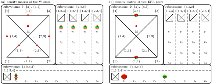
Figure 2: (a) Visualizations of the density matrix $|W\rangle\langle W|$ of the four-qubit W state $|W\rangle$, the droplet function for the subsystem $\{1,\!2,\!3,\!4\}$ is scaled to 2/3 of its original size. (b) Visualizations of the density matrix $|\psi\rangle\langle\psi|$ of two EPR pairs $|\psi\rangle=(|0000\rangle+|1111\rangle+|0011\rangle+|1100\rangle)/2$ (between spins 1 and 2 as well as 3 and 4).

The left part of Table 2 describes the decomposition of the tensor space. For each subsystem size $g$, we list the potentially occurring partitionsBoerner (1967); Hamermesh (1962); Pauncz (1995); Sagan (2001) $\lambda$ and the associated tableaux $\tau_{i}^{[g]}$, which are given together with their quantity and index. Also, for each $\lambda$ we state the appearing tensor ranks $j$. The bilinear tensors for a fixed subsystem $G\in\binom{\{1,..,4\}}{2}$ are combined into a single droplet function, which is possible as the relevant ranks $0$, $2$, and $1$ do not contain any repetition. Note that for $g=4$, the partition [1,1,1,1] and its tableau $\tau_{10}^{[6]}$ do not correspond to any rank $j$ (indicated by “-” at the bottom of the last column of the table at the left side of Tab. 2). For each of the possible subsystems $G\in\binom{\{1,..,4\}}{g}$, we have in total one label for the zero-linear tensor, one label for linear tensors, one label for bilinear tensors, four labels for trilinear tensors, and nine labels for four-linear tensors. This labeling structure for a system of four spins $1/2$ is reflected on the right of Table 2, where a $16\times 16$ complex random matrix is visualized using multiple droplet functions. The upper left panel on the right of Table 2 highlights the topology of the spin system, where nodes represent single spins $1/2$ and edges correspond to bilinear tensors. Each droplet $f^{(\ell)}$ is arranged according to its label $\ell$. The visualization of the zero-linear tensor is labeled by $\ell=\mathrm{Id}$, linear tensors by their subsystem $\ell=\{a\}$ for $a\in\{1,..,4\}$, and bilinear tensors also by their subsystem $\ell=\{a,\!b\}$ for $a,b\in\{1,..,4\}$ with $a<b$, i.e., $\ell\in\{\{1,\!2\},\{1,\!3\},\{1,\!4\},\{2,\!3\},\{2,\!4\},\{3,\!4\}\}$. We use $\ell=(G,\tau_{i}^{[g]})$ for $3\leq g\leq 4$, which explicitly specifies the tableau $\tau_{i}^{[g]}$. On the right of Table 2, we also see the labels given by the four tableaux $\tau_{i}^{[3]}$ for each of the trilinear subsystems $G\in\{\{1,\!2,\!3\},\{1,\!2,\!4\},\{1,\!3,\!4\},\{2,\!3,\!4\}\}$, where the edges between involved spins are indicated by bold black lines whereas edges to non-involved spins are grayed out. In the four-linear subsystem $\{1,\!2,\!3,\!4\}$, non-zero droplet functions can only occur for the nine tableaux $\tau_{1}^{[4]}$-$\tau_{9}^{[4]}$. Hence in a system consisting of four spins $1/2$, the information contained in an arbitrary operator (consisting of $(2^{4})^{2}=256$ complex matrix elements) is represented by 36 droplet functions, which have the correct transformation properties under non-selective rotations and which are organized according to the subset $G$ of involved spins and the type of permutation symmetry specified by a Young tableau $\tau_{i}^{[g]}$.

The cases of $g=5$ and $g=6$ are detailed in Table LABEL:tab:tableaux and visualizations of a complex random matrix for systems consisting of five and six spins $1/2$ are shown in Figs. 9 and LABEL:fig:6spin_1d2 of Appendix A.3, respectively. For subsystem sizes $g\geq 6$, in addition to the set $G$ of involved spins and the Young tabeleau $\tau_{i}^{[g]}$, the label $\ell$ for a given droplet function may also include an additional ad hoc sublabel $\mathcal{A}$, resulting in $\ell=(G,\tau_{i}^{[g]},\mathcal{A})$.

Next, two examples illustrate how inherent symmetries of density matrices are made apparent in our visualization approach. We consider two entangled pure statesDür, Vidal, and Cirac (2000); Briegel and Raussendorf (2001); Verstraete et al. (2002) in a four-qubit system (i.e. a system consisting of four spins $1/2$), where the corresponding density matrices are highlighted in Fig. 2 following exactly the prototype in Table 2. The first example is shown in Fig. 2(a), which represents the density matrix $|W\rangle\langle W|$ of the four-qubit W stateDür, Vidal, and Cirac (2000); Briegel and Raussendorf (2001) $|W\rangle=(|0001\rangle+|0010\rangle+|0100\rangle+|1000\rangle)/2$, which is also known as a Dicke state.Dicke (1954); Stockton et al. (2003) The highly symmetric structure of $|W\rangle\langle W|$ is clearly visible in Fig. 2(a). All droplet functions for different subsystems $G$ of a given linearity $g$ have an identical shape. Also, only the fully permutation symmetric tensors corresponding to the tableaux $\tau_{1}^{[2]}$, $\tau_{1}^{[3]}$, and $\tau_{1}^{[4]}$ appear. In total, only 16 droplet functions are nonzero. This is reflected by the tensor decomposition

$$|W\rangle\langle W|= \;T_{00}^{\text{Id}}-\tfrac{1}{2}\sum_{k=1}^{4}T_{10}^{\{k\}}+\left(\sum_{\{k,l\}\in G_{2}}\tfrac{1}{\sqrt{3}}T_{00}^{\{k,l\}}-\tfrac{1}{\sqrt{6}}T_{20}^{\{k,l\}}\right)$$

$$+\left(\sum_{\{k,l,m\}\in G_{3}}-\tfrac{3}{\sqrt{60}}T_{10}^{(\{k,l,m\},\tau_{1}^{[3]})}+\tfrac{4}{\sqrt{10}}T_{30}^{(\{k,l,m\},\tau_{1}^{[3]})}\right)+\left(\tfrac{2}{\sqrt{20}}T_{00}^{\tau_{1}^{[4]}}-\tfrac{1}{\sqrt{7}}T_{20}^{\tau_{1}^{[4]}}-\tfrac{16}{\sqrt{70}}T_{40}^{\tau_{1}^{[4]}}\right)$$

with $G_{2}=\{\{1,\!2\},\{1,\!3\},\{1,\!4\},\{2,\!3\},\{2,\!4\},\{3,\!4\}\}$ and $G_{3}=\{\{1,\!2,\!3\},\{1,\!2,\!4\},\{1,\!3,\!4\},\{2,\!3,\!4\}\}$.

The second example is given by the density matrix $|\psi\rangle\langle\psi|$ of two EPR pairsVerstraete et al. (2002) $|\psi\rangle=(|0000\rangle+|1111\rangle+|0011\rangle+|1100\rangle)/2$ and is illustrated in Fig. 2(b). Again, the symmetry structure of $|\psi\rangle\langle\psi|$ is readily visible. In this case, linear and trilinear droplet functions are completely absent. For the bilinear droplet functions, only the ones corresponding to the subsystems $\{1,\!2\}$ and $\{3,\!4\}$ are nonzero as the qubits 1 and 2 as well as 3 and 4 form the EPR pairs. In the second example, we obtain the tensor decomposition

$$|\psi\rangle\langle\psi|= \;T_{00}^{\text{Id}}+\left(\tfrac{1}{\sqrt{3}}T_{00}^{\{1,2\}}+T_{2,-2}^{\{1,2\}}+\tfrac{2}{\sqrt{6}}T_{20}^{\{1,2\}}+T_{2,2}^{\{1,2\}}\right)+\left(\tfrac{1}{\sqrt{3}}T_{00}^{\{3,4\}}+T_{2,-2}^{\{3,4\}}+\tfrac{2}{\sqrt{6}}T_{20}^{\{3,4\}}+T_{2,2}^{\{3,4\}}\right)$$

$$+\left[\tfrac{7}{\sqrt{45}}T_{00}^{\tau_{1}^{[4]}}{+}\tfrac{2}{\sqrt{63}}T_{20}^{\tau_{1}^{[4]}}{+}\tfrac{6}{\sqrt{70}}T_{40}^{\tau_{1}^{[4]}}{+}\tfrac{2}{\sqrt{42}}\left(\sqrt{6}T_{4,-2}^{\tau_{1}^{[4]}}{+}T_{2,-2}^{\tau_{1}^{[4]}}{+}T_{22}^{\tau_{1}^{[4]}}{+}\sqrt{6}T_{4,2}^{\tau_{1}^{[4]}}\right)+T_{4,-4}^{\tau_{1}^{[4]}}+T_{44}^{\tau_{1}^{[4]}}\right]$$

$$-\left[\tfrac{2}{3}T_{00}^{\tau_{5}^{[4]}}+\tfrac{4}{\sqrt{18}}T_{20}^{\tau_{5}^{[4]}}+\tfrac{2}{\sqrt{3}}\left(T_{2,-2}^{\tau_{5}^{[4]}}+T_{22}^{\tau_{5}^{[4]}}\right)\right],$$

which explains the occurrence of four-linear components in Fig. 2(b) even though the state $|\psi\rangle$ is a product state and has no four-particle contributions as a pure state. This emphasizes the fact that the DROPS visualization does not (directly) depict the symmetries of a pure state $|\psi\rangle$ but of the corresponding density-matrix $|\psi\rangle\langle\psi|$.

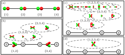
Figure 3: Generation of a completely symmetric four-linear state in a chain of four spins $1/2$ following Table S2 in Ref. Köcher et al., 2016. Starting from $\rho_{0}=\sum_{k=1}^{4}I_{kz}$ a $[\pi/2]_{y}$ pulse on each spin results in (a), the evolution under coupling with time $t=1/(2\mathrm{J})$ followed by a $[\pi/2]_{y}$ pulse on each spin is repeating three times and visualized at various stages (b)-(d). The droplet function in (d) is scaled to 1/3 of its original size. Linear and bilinear droplet functions are plotted on the nodes (i.e. spins) and edges (i.e. couplings), respectively. General $g$-linear components are indicated by dashed ellipses. Note (2)

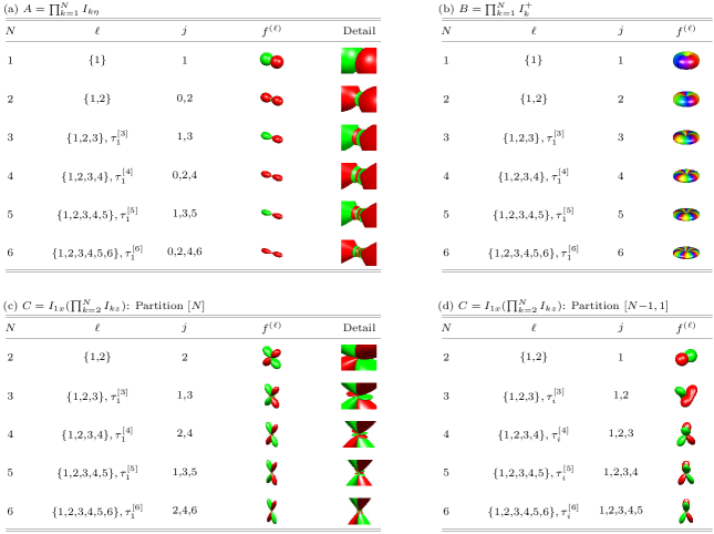
Figure 7: The droplet functions $f^{(\ell)}$ visualizing various operators for up to six coupled spins $1/2$ ($N=6$). The full labels are given in the second column and the occurring tensors ranks $j$ are shown in the third column of each table. The detail column shows the corresponding magnified centers of $f^{(\ell)}$. In Table (a), the spherical functions $f^{(\ell)}$ of the fully symmetrical operator $A=\prod_{k=1}^{N}I_{kx}$ are shown. Table (b) depicts the representations of the non-Hermitian operators $B=\prod_{k=1}^{p}I^{+}_{k}$. In Table (c) and (d), the visualizations of the antiphase operators $C=I_{1x}(\prod_{k=2}^{N}I_{kz})$ are depicted. There is only one symmetry type $\tau_{1}^{[N]}$ for the partition $[N]$ and the related droplet is shown in Table (c) . For the partition $[N{-}1,1]$, we find $N{-}1$ different standard Young tableaux $\tau_{i}^{[N]}$ with $i\in\{2,\dots,N\}$ and thus, have $N{-}1$ droplets $f^{(\ell)}$. They all have identical shapes but different sizes and one representative spherical function for this case is illustrated in Table (d). In total $N$ droplets visualize the antiphase operator from Eq. (33). In contrast to our usual strategy, droplets for two spins (i.e. $N=2$) are plotted here separately for the fully permutation-symmetric part (i.e. for the partition $[N]$) in (c) and the remaining part in (d).

The last example in this section illustrates the value of the DROPS visualization for analyzing the dynamics of controlled quantum systems.Glaser et al. (2015) This enables us to analyze the effect of control schemes by illustrating the droplets and their symmetries appearing during the time evolution. A free simulation packageGlaser, Tesch, and Glaser (2015); Tesch, Glaser, and Glaser (2018) is available, which can be used to simulate systems consisting of up to three spins $1/2$. In the context of nuclear magnetic resonance spectroscopy, we consider the creation of maximum-quantum coherence in an Ising chain of four spins $1/2$ (see Fig. 3), which is based on a $\pi/2$ excitation pulse followed by a series of delays and $\pi/2$ pulses.Köcher et al. (2016) An operator $A_{p}$ has a defined coherence orderErnst, Bodenhausen, and Wokaun (1987) $p$ if a rotation around the $z$ axis by any angle $\alpha$ generates the same operator $A_{p}$ up to a phase factor $\exp(-ip\alpha)$, i.e., $\exp(-i\alpha\sum_{k=1}^{N}I_{kz})A_{p}\exp(i\alpha\sum_{k=1}^{N}I_{kz})=A_{p}\exp(-ip\alpha)$. Recall that Cartesian operators for single spins are $I_{x}:=\sigma_{x}/2$, $I_{y}:=\sigma_{y}/2$, and $I_{z}:=\sigma_{z}/2$, where the Pauli matrices are $\sigma_{x}=\left(\begin{smallmatrix}0&1\\ 1&0\end{smallmatrix}\right)$, $\sigma_{y}=\left(\begin{smallmatrix}0&-i\\ i&0\end{smallmatrix}\right)$, and $\sigma_{z}=\left(\begin{smallmatrix}1&0\\ 0&-1\end{smallmatrix}\right)$. For $n$ spins, one has the operators $I_{k\eta}:=\bigotimes_{s=1}^{n}I_{a_{s}}$ where $a_{s}$ is equal to $\eta$ for $s{=}k$ and is zero otherwise; note $I_{0}:=\left(\begin{smallmatrix}1&0\\ 0&1\end{smallmatrix}\right)$. All tensor-operator components $T_{jm}$ have the unique coherence order $p=m$. The Cartesian product operator $I_{kx}$, which corresponds to observable transverse magnetization, contains coherence order $p=\pm 1$ and a triple-quantum coherence state is a linear combination of tensor operators with rank $j\geq 3$ and order $m=\pm 3$. The maximal coherence order is limited by the number of spins and thus by the maximal rank $j$ of tensors. Note that a droplet $f^{(\ell)}$ representing an operator $A_{p}$ with coherence order $p$ exhibits the same rotation properties as $A_{p}$. That is $f^{(\ell)}$ is reproduced up to a phase factor $\exp(-ip\alpha)$ if $f^{(\ell)}$ is rotated around the $z$ axis by $\alpha$, refer also to Fig. 7. The experiment considered in Ref. Köcher et al., 2016 generates maximal quantum coherence states starting from the initial state $\rho_{0}=\sum_{k=1}^{4}I_{kz}$, which is specified using the Cartesian product operators $I_{kz}$. All coupling constants in the drift (or system) Hamiltonian are assumed to be equal, i.e., $\mathrm{J}=\mathrm{J}_{12}=\mathrm{J}_{23}=\mathrm{J}_{34}$. In a first step, a $[\pi/2]_{y}$ pulse is applied on each spin. Then, a transfer block consisting of an evolution under the coupling with coupling period $t=1/(2\mathrm{J})$ followed by a $[\pi/2]_{y}$ pulse on each spin is repeated three times. The panels in Fig. 3 show the state of the spin system for different points in time: Panel (a) represents the initial state $\rho_{0}=\sum_{k=1}^{4}I_{kz}$ after a $\pi/2$ pulse with phase $y$ is applied to each spin. Panels (b), (c), and (d) depict the state after one, two, and three repetitions of the transfer block, respectively. In panel (d), the initial state has been fully transferred to a single 4-linear droplet function corresponding to fully permutation-symmetric tensors (as denoted by $\tau_{1}^{[4]}$), which also contains the desired maximum-coherence ordersKöcher et al. (2016) $p=\pm 4$. A similar example for an Ising chain consisting of five spins $1/2$ is shown in Appendix A.2 [refer to Fig. 8(a1)-(a5)].

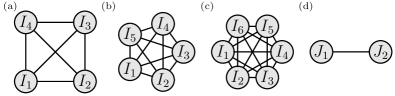
Figure 4: Interaction structure of visualized spin systems (nodes represent spins): (a)-(c) systems with $N\in\{4,5,6\}$ spins $1/2$ (see Sec. IV), (d) two spins with arbitrary spin numbers $J_{1}$ and $J_{2}$ as discussed in Sec. V.

Additional examples and applications of the DROPS visualization are illustrated in Appendix A. In Fig. 4(a)-(c), general systems consisting of four to six spins $1/2$ are schematically represented as complete graphs. In the following, we discuss the generalization of the DROPS representation to systems consisting of two, see Fig. 4(d), or more spins with arbitrary spin numbers.

V Representation of systems consisting of spins with arbitrary spin numbers

Building on our description in Sec. II, we now consider the case of two coupled spins with arbitrary spin numbers. Even though spins $1/2$ (which are also known as qubits) constitute the most important case, spins with higher spin number $J>1/2$ are highly relevant and widely studied as exemplified by bosonic systems, such as photons and gluons, composite particles as deuterium or helium-4, and quasiparticles such as Cooper pairs or phonons. We start in Sec. V.1 with the case of two coupled spins with arbitrary but identical spin number $J$. We extend this case to two coupled spins with different spin numbers $J_{1}\neq J_{2}$ in Sec. V.2, which also discusses examples and illustrations for the concrete spin numbers $J_{1}=1/2$ and $J_{2}=1$. Generalizations of our approach to an arbitrary number of coupled spins with arbitrary spin numbers are discussed in Sec. V.3.

Table 3: Multiplicities of ranks $j$ occurring for bilinear tensors in two-spin systems with equal spin numbers $J_{1}=J_{2}=J$ (left) and different spin numbers $J_{1}\neq J_{2}$ (right).

$J$ $\lambda$ $j=$ $0$ $1$ $2$ $3$ $4$ $5$ $6$ $7$ $8$ $9$ $10$ $11$ $12$ $13$ $14$ $1/2$ [2] 1 1 [1,1] 1 $1$ [2] 2 1 3 1 1 [1,1] 3 1 2 $3/2$ [2] 3 2 6 3 4 1 1 [1,1] 5 3 5 2 2 $2$ [2] 4 3 9 6 8 4 4 1 1 [1,1] 7 5 9 5 6 2 2 $5/2$ [2] 5 4 12 9 13 8 9 4 4 1 1 [1,1] 9 7 13 9 11 6 6 2 2 $3$ [2] 6 5 15 12 18 13 15 9 9 4 4 1 1 [1,1] 11 9 17 13 17 11 12 6 6 2 2 $7/2$ [2] 7 6 18 15 23 18 22 15 16 9 9 4 4 1 1 [1,1] 13 11 21 17 23 17 19 12 12 6 6 2 2

$J_{1}$ $J_{2}$ $j=$ $0$ $1$ $2$ $3$ $4$ $5$ $6$ $7$ $8$ $9$ $10$ $11$ $1/2$ $1$ 1 2 2 1 $1/2$ $3/2$ 1 2 3 2 1 $1/2$ $2$ 1 2 3 3 2 1 $1/2$ $5/2$ 1 2 3 3 3 2 1 $1/2$ $3$ 1 2 3 3 3 3 2 1 $1/2$ $7/2$ 1 2 3 3 3 3 3 2 1 $1$ $3/2$ 2 5 6 5 3 1 $1$ $2$ 2 5 7 7 5 3 1 $1$ $5/2$ 2 5 7 8 7 5 3 1 $1$ $3$ 2 5 7 8 8 7 5 3 1 $1$ $7/2$ 2 5 7 8 8 8 7 5 3 1 $3/2$ $2$ 3 8 11 11 9 6 3 1 $3/2$ $5/2$ 3 8 12 13 12 9 6 3 1 $3/2$ $3$ 3 8 12 14 14 12 9 6 3 1 $2$ $5/2$ 4 11 16 18 17 14 10 6 3 1 $2$ $3$ 4 11 17 20 20 18 14 10 6 3 1

Table 4: Labeling scheme for bilinear tensors of two coupled spins. For $J_{1}=J_{2}=J$ (left), parent sublabels $\mathcal{P}$ and Young tableaux sublabels $\tau_{i}^{[g]}$ are used. For $J_{1}\neq J_{2}$ (right), Young tableaux are replaced by ad hoc sublabels. Both cases result in $4J_{1}J_{2}$ droplet functions.

$\mathcal{P}$ $\tau_{i}^{[g]}$ $j$ $\ell$  ($J_{1}=J_{2}=J$) $1$,$1$ $\tau_{1}$ $0$,$2$}1.811pt $\{1,\!2\},1,1$ $\tau_{2}$ $1$ $2$,$2$ $\tau_{1}$ $0$,$2$,$4$}1.811pt $\{1,\!2\},2,2$ $\tau_{2}$ $1$,$3$ $\vdots$ $\vdots$ $\vdots$ $2J$,$2J$ $\tau_{1}$ $0$,$2$,$4$,..,$2J$  }1.811pt $\{1,\!2\},2J,2J$ $\tau_{2}$ $1$,$3$,..,$2J{-}1$ $1$,$2$ $\tau_{1}$ $1$,$2$,$3$ $\{1,\!2\},1,2,\tau_{1}$ $\tau_{2}$ $1$,$2$,$3$ $\{1,\!2\},1,2,\tau_{2}$ $\vdots$ $\vdots$ $\vdots$ $k$,$l$   $(l\neq k)$ $\tau_{1}$ $|k{-}l|$,..,$k{+}l$ $\{1,\!2\},k,l,\tau_{1}$ $\tau_{2}$ $|k{-}l|$,..,$k{+}l$ $\{1,\!2\},k,l,\tau_{2}$ $\vdots$ $\vdots$ $\vdots$ $2J{-}1$,$2J$ $\tau_{1}$ $1$,..,$2J{-}1$ $\{1,\!2\},2J{-}1,2J,\tau_{1}$ $\tau_{2}$ $1$,..,$2J{-}1$ $\{1,\!2\},2J{-}1,2J,\tau_{2}$

$\mathcal{P}$ $\mathcal{A}$ $j$ $\ell$  ($J_{1}\neq J_{2}$) $1,1$ $0,1,2$ $\{1,\!2\},1,1$ $2,2$ $0,1,2,3,4$ $\{1,\!2\},2,2$ $\vdots$ $\vdots$ $2J_{1},2J_{1}$ $0$,..,$4J_{1}$ $\{1,\!2\},2J_{1},2J_{1}$ $2,3$ $I$ $1$,..,$5$ $\{1,\!2\},2,3,I$ $II$ $1$,..,$5$ $\{1,\!2\},2,3,II$ $\vdots$ $\vdots$ $k,l$  $(l>k)$ $I$ $l{-}k$,..,$l{+}k$ $\{1,\!2\},k,l,I$ $II$ $l{-}k$,..,$l{+}k$ $\{1,\!2\},k,l,II$ $\vdots$ $\vdots$ $2J_{1}{-}1,2J_{1}$ $I$ $1$,..,$2J_{1}{-}1$ $\{1,\!2\},2J_{1}{-}1,2J_{1},I$ $II$ $1$,..,$2J_{1}{-}1$ $\{1,\!2\},2J_{1}{-}1,2J_{1},II$ $2J_{1},2J_{1}{+}1$ $1$,..,$2J_{1}+1$ $\{1,\!2\},2J_{1},2J_{1}{+}1$ $\vdots$ $\vdots$ $2J_{1},2J_{2}$ $2J_{1}{-}2J_{2}$,..,$2J_{1}{+}2J_{2}$ $\{1,\!2\},2J_{1},2J_{2}$

V.1 Two coupled spins with equal spin numbers

Recall from Sec. II that the state of a single spin $J$ can be described by $2J{+}1$ tensor operators $T_{j}$ with ranks $j\in\{0,\dots,2J\}$ where each tensor operator $T_{j}$ has $2j{+}1$ tensor-operator components $T_{jm}\in\mathbb{C}^{(2J+1)\times(2J+1)}$ with $m\in\{-j,\dots,j\}$. The rank $j=0$ corresponds to a zero-linear tensor operator and the ranks $1\leq j\leq 2J$ correspond to linear tensor operators. Compared to the case of spins $1/2$, the number and multiplicity of the occurring ranks $j$ in tensor decompositions for multiple spins grow even more rapidly for general spin numbers. This is already appreciable for bilinear tensors of two spins as detailed for different values of $J_{1}=J_{2}=J$ on the left of Table 3, where multiplicities of the occurring ranks are listed separately for the permutation symmetries corresponding to the partitions [2] and [1,1]. Additional sublabels are required to distinguish between multiply appearing ranks $j$ in order to maintain the bijectivity of the mapping from tensor operators to spherical harmonics following Sec. II.

For two coupled spins, there are zero-linear, linear, and bilinear tensors as given by the different numbers $g\in\{0,1,2\}$ of involved spins. The treatment of the cases with $g\in\{0,1\}$ follows Sec. II. For $g=0$, the set $G=\emptyset$ of involved spins is empty. The corresponding single zero-linear tensor operator of rank $j=0$ requires no further partitioning and is given the label $\ell=\text{Id}$. The linear tensors are partitioned according to the set $G\in\{\{1\},\{2\}\}$ of involved spins, which contains either the first or the second spin. For both cases, $2J$ linear tensor operators with ranks $j\in\{1,2,\dots,2J\}$ are present and no rank appears twice. This ensures that no additional sublabels are necessary and the labels $\ell=\{1\}$ and $\ell=\{2\}$ can be used to uniquely specify the linear tensor operators. So far, the tensor operators corresponding to the labels $\ell\in\{\text{Id},\{1\},\{2\}\}$ result jointly in three droplet functions.

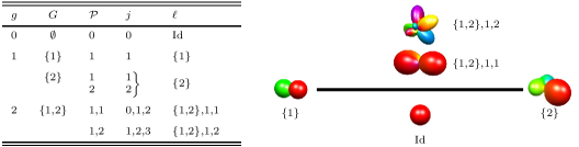
Figure 5: The labeling scheme for two spins with spin numbers $J_{1}=1/2$ and $J_{2}=1$ results in five groups of tensors (left). The right panel visualizes the corresponding droplet functions for a $6\times 6$-dimensional complex random matrix.

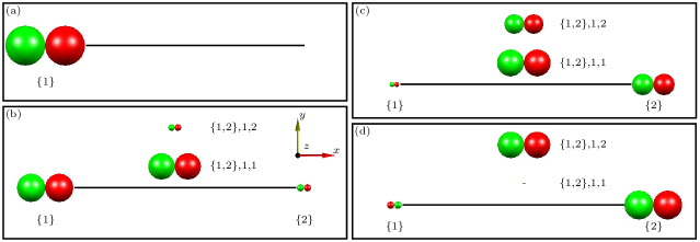
Figure 6: Visualization of a negative polarization transfer under isotropic mixing conditions in a two-spin system consisting of a spin $1/2$ and a spin $1$ (see Ref. Luy and Glaser, 2000): (a) 0 ms, (b) 10 ms, (c) 20 ms, and (d) 30 ms.

For bilinear tensors, the occurring ranks $j$ and their multiplicity are detailed on the left of Table 3 separately for the partitions [2] and [1,1]. Additional sublabels are necessary for $J>1/2$ to uniquely distinguish the appearing tensor operators. This is also true after the sublabels for permutation symmetries given by the partitions [2] and [1,1] (or the related Young tableaux $\tau_{i}$) have been applied. Ad hoc sublabels could be used, but they usually do not correlate with any physical properties of the quantum system. Instead, here we employ so-called parent sublabels (or parents), which are motivated by classical methods.Condon and Shortley (1935); Racah (1942, 1943, 1949); Elliott and Lane (1957); Racah (1965); Kaplan (1975); Chisholm (1976); Kramer, John, and Schenzle (1981); Rowe and Wood (2010) Recall that a bilinear tensor operator $T_{j}$ of rank $j$ is obtained in the Clebsch-Gordon decomposition [see Eq. (7)] from the tensor product of the two linear tensor operators $T_{j_{1}}$ and $T_{j_{2}}$. The ranks $j_{1}$ and $j_{2}$ (with $j_{1}\leq j_{2}$) form the parent sublabel $\mathcal{P}=(j_{1},\!j_{2})$ of $T_{j}$. For example, the bilinear tensor operator $T_{1}$ appears in the decomposition of $T_{1}\otimes T_{2}$. This results in the parent sublabel (or parents) $\mathcal{P}=(1,\!2)$ for this bilinear tensor operator $T_{1}$, representing the ranks $j_{1}=1$ and $j_{2}=2$ of the linear tensor operators $T_{1}$ and $T_{2}$. One significant advantage of using parent sublabels is that they naturally arise in the construction of tensor operators. All parents that appear for bilinear tensors of two coupled spins with arbitrary but equal spin number are detailed on the left-hand side of Table 4. The bilinear tensors are grouped according to their parents and their Young tableaux $\tau_{i}$, which specify permutation symmetries as discussed above. This scheme results in $(2J)^{2}$ droplet functions representing bilinear tensors. In total, $(2J)^{2}+3$ droplet functions are needed to completely specify the quantum state of two coupled spins with identical spin number $J$. Recall that for two coupled spins $1/2$ (i.e. with $J_{1}=J_{2}=J=1/2$), bilinear tensors can be uniquely represented by only one ($(2J)^{2}=1$) droplet function, which is fully specified by the label $\ell=G=\{1,2\}$, which indicates that it contains operators acting on the first and second spin. However, for two coupled spins with $J_{1}=J_{2}=J^{\prime}=1$, four ($(2J^{\prime})^{2}=4$) droplet functions are necessary to represent all bilinear tensors, which obviously are not uniquely specified by the set $G=\{1,2\}$ of involved spins. Of these four bilinear droplet functions, two function have identical parent ranks ($j_{1}=j_{2}$) and are fully characterized by a label of the form $\ell=(G,\mathcal{P})$: the complete label for $j_{1}=j_{2}=1$ is $(\{1,\!2\},1,1)$ and $(\{1,\!2\},2,2)$ for $j_{1}=j_{2}=2$. The two remaining bilinear droplet functions have parent ranks $j_{1}=1$ and $j_{2}=2$ but different Young tableaux $\tau_{i}$. They are fully specified by the labels $(\{1,\!2\},1,2,\tau_{1})$ and $(\{1,\!2\},1,2,\tau_{2})$, respectively (c.f. fourth column in Table 4).

V.2 Two coupled spins with different spin numbers

Building on the methodology introduced in Sec. V.1, we address in this section the case of two coupled spins with different spin numbers $J_{1}\neq J_{2}$. As before, the appearing bilinear tensor ranks $j$ and their multiplicity grows rapidly as shown on the right of Table 3. Zero-linear and linear tensors can be—as before—represented using three droplet functions. In contrast to the case of equal spin numbers, we can no longer rely on permutation symmetries to label bilinear droplet functions, because permuting spins with different spin numbers does not preserve the global structure of the quantum system. This forces us to combine parent sublabels with ad hoc sublabels in order to completely subdivide all bilinear tensors. The resulting labeling scheme for bilinear tensors is summarized on the right of Table 4. Overall, $4J_{1}J_{2}$ different droplet functions exist for bilinear tensors and arbitrary operators are represented by $4J_{1}J_{2}+3$ droplet functions.

A concrete example is given in Fig. 5 for the case of two coupled spins with the spin numbers $J_{1}=1/2$ and $J_{2}=1$. The labeling scheme is detailed on left of Fig. 5. One observes the tensor rank of zero for the zero-linear tensors, the linear tensor rank of one for the spin $1/2$, and the linear tensor ranks of one and two for the spin $1$. The bilinear tensor ranks are given by zero, one, and two for the parent sublabel $P=(1,\!1)$ as well as one, two, and three for the parent sublabel $P=(1,\!2)$. The right panel of Fig. 5 shows the corresponding droplet functions, which are arranged according to their labels.

For the same case of one spin $1/2$ and one spin $1$, we visualize in Fig. 6 the dynamics of quantum states during an isotropic mixing polarization transfer experiment. In this experiment, $x$ polarization of the first spin (represented by droplet $\{1\}$), which corresponds to the initial density operator $S_{1x}$, is transferred via bilinear operators [represented by the droplets $(\{1,\!2\},1,1)$ and $(\{1,\!2\},1,1)$] to $x$ polarization of the second spin (represented by droplet $\{2\}$) under the effective isotropic mixing (Heisenberg) coupling Hamiltonian $H_{\text{iso}}=2\pi\mathrm{J}_{\text{iso}}(S_{1x}S_{2x}+S_{1y}S_{2y}+S_{1z}S_{2z})$.Luy and Glaser (2000) The operators in this case are defined by $S_{1\eta_{1}}:=I_{\eta_{1}}\otimes\text{id}_{3}$ and $S_{2\eta_{2}}:=\text{id}_{2}\otimes S_{\eta_{2}}$, where

$$S_{x}=\tfrac{1}{\sqrt{2}}\left(\begin{smallmatrix}0&1&0\\ 1&0&1\\ 0&1&0\end{smallmatrix}\right),\quad S_{y}=\tfrac{1}{\sqrt{2}i}\left(\!\!\begin{smallmatrix}\phantom{-}0&\phantom{-}1&\phantom{-}0\\ -1&\phantom{-}0&\phantom{-}1\\ \phantom{-}0&-1&\phantom{-}0\end{smallmatrix}\right),\quad\text{and}\quad S_{z}=\left(\begin{smallmatrix}1&\phantom{-}0&\phantom{-}0\\ 0&\phantom{-}0&\phantom{-}0\\ 0&\phantom{-}0&-1\end{smallmatrix}\right)$$

are the spin-$1$ matrices and $\text{id}_{n}$ denotes the $n\times n$ identity matrix. For a coupling constant $\mathrm{J}_{\text{iso}}$ of $11$ Hz, the four panels in Fig. 6 show DROPS representations of the density matrix after (a) 0 ms, (b) 10 ms, (c) 20 ms, and (d) 30 ms, respectively. The time-dependent $x$ polarization of the first spin is given by the function $T_{1x}(t)=\{11+16\cos(3\pi\mathrm{J}_{\text{iso}}\,t)\}/18$, which is negative for $t$=30 ms. This is visible in panel (d), where the sign of the linear droplet corresponding to the first spin (labeled $\{1\}$) is inverted compared to panels (a) to (c): Whereas initially, the positive (red) lobe of the droplet $\{1\}$ points in the positive $x$ direction, after 30 ms the positive (red) lobe of the droplet $\{1\}$ points in the negative $x$ direction. The occurrence of polarization with inverted sign in such a simple two-spin system (consisting of a spin $1/2$ and a spin $1$) is of interestLuy and Glaser (2000) because at least five spins are necessary to achieve negative polarization in isotropic mixing experiments in systems consisting exclusively of spins $1/2$.

V.3 Generalization to an arbitrary number of spins with arbitrary spin numbers

We discuss now how parent sublabels can be also applied to more than two spins. The most general spin system is composed of an arbitrary number of coupled spins with arbitrary spin numbers $J_{k}$. The zero-linear and linear tensors can be described as before. In particular, one has $2J_{k}$ linear tensors with rank $j\in\{1,\dots,2J_{k}\}$. Bilinear and general $g$-linear tensors can be initially divided with respect to the set $G$ of involved spins. A $g$-linear tensor operator $T_{j}$ is obtained via repeated Clebsch-Gordan decompositions from $g$ linear tensor operators $T_{j_{k}}$ of rank $j_{k}$ with $1\leq k\leq g$. And the parent sublabel $\mathcal{P}=(j_{1},\!j_{2},\ldots,\!j_{g})$ of $T_{j}$ is given by the sequence of ranks. For example, the trilinear tensor operator $T_{2}$ is contained in the Clebsch-Gordon decomposition of the tensor product of the three linear tensor operators $T_{1}$, $T_{1}$, and $T_{2}$ and its parent sublabel is given by $\mathcal{P}=(1,\!1,\!2)$. Young tableaux specifying permutation symmetries could be at least applied to subsystems with equal spin numbers. Theoretically, ad hoc sublabels can always be used to discern between any remaining tensor operators with equal rank. However, the practicability of this approach, which is related to the scaling of the number of necessary ad hoc sublabels, has to be investigated in future work together with the option of subgroup labels.Condon and Shortley (1935); Racah (1942, 1943, 1949); Elliott and Lane (1957); Racah (1965); Kaplan (1975); Chisholm (1976); Kramer, John, and Schenzle (1981); Rowe and Wood (2010)

VI Explicit construction of the symmetry-adapted bases

Here, we present the details for constructing symmetry-adapted bases as outlined in Sec. III. Each tensor operator has to be uniquely identified by a set of sublabels (or quantum numbers). After the space of all tensors has been divided according to their $g$-linearity and the subsystem $G$ of involved spins, the tensors can be further subdivided with respect to their parents $\mathcal{P}$ (as introduced in Sec. V), their permutation symmetries as given by a Young tableau $\tau^{[g]}$ of size $g$, and/or necessary ad hoc sublabels $\mathcal{A}$ that together with the rank $j$ and order $m\in\{-j,\ldots,j\}$ finally identify a one-dimensional tensor subspace. Some of this information might be redundant or inapplicable in certain cases (as permutation symmetries in the scenario of Sec. V.2), and we also do not utilize parent sublabels in spin-$1/2$ systems. Our explanations start below with the initial construction of zero-linear and linear tensors. In Sec. VI.1 and Sec. VI.2, we then separately describe the iterative construction of $g$-linear tensor operators (for $g\geq 2$) based on the projection method (denoted as Method A in Sec. III) and on the CFP method relying on fractional parentage coefficients (denoted as Method B in Sec. III). We conclude by explaining the chosen phase convention for DROPS basis tensor operators (see Sec. VI.3) and how tensors are embedded into a full $N$-spin system (see Sec. VI.4).

Let us first recall the tensor-operator notation $T_{jm}^{(G,\mathcal{P},\tau,\mathcal{A})}$, which uses the rank $j$ and order $m$ together with all possible sublabels given by the set $G$ of involved spins, the parent sublabel $\mathcal{P}$, the permutation symmetry $\tau$, and the ad hoc sublabel $\mathcal{A}$. Below, a superscript $[g]$ is used for each sublabel to indicate a specific linearity $g$. Before accounting for the embedding in Sec. VI.4, the label $G^{[g]}$, is dropped. By default, we assume that for a $g$-linear term the set of spins consists of the first $g$ spins of the system, i.e. $G^{[g]}=\{1,\ldots,g\}$ for a linearity $g\geq 1$ and $G^{[0]}=\emptyset$.

In the zero-linear case ($g=0$), the parent sublabel is an empty list $\mathcal{P}^{[0]}=()$, the tableau sublabel is empty ($\tau^{[0]}=\varnothing$), and the ad hoc label is canonically initialized to $\mathcal{A}^{[0]}=I$; also $j^{[0]}=0$ and $m^{[0]}=0$. We use the abbreviations $T_{0}$ and $T_{00}$ for the tensor operator and its component in the zero-linear case, while emphasizing that their explicit form depends on the spin number $J$ as detailed in Eqs. (4) and (6).

For the case of linear tensors, $\mathcal{P}^{[1]}=(j^{[1]})$ for the rank $j^{[1]}$, $\tau^{[1]}=\ytableaushort{1}$, and $\mathcal{A}^{[1]}=I$. The linear tensor operators and their components can be uniquely identified using the simplified notations $T_{j}$ and $T_{jm}$ with $j=j^{[1]}\neq 0$. Their explicit form depends again on the spin number $J$, see Eqs. (5) and (6). After addressing these notational issues and default initializations, we discuss the iterative construction process.

VI.1 Projection method

In the first phase of the projection method, the tensor decomposition from Eq. (9) is iteratively applied in order to construct $g$-linear tensors from $(g{-}1)$-linear ones as outlined in Sec. III and Fig. 1. The explicit form of the corresponding tensor components can be computed with the help of Eq. (8) and the knowledge of Clebsch-Gordan coefficients. During this iteration the Young-tableau sublabels are ignored since permutation symmetries are only accounted for in the second and third phase of the projection method. Ad hoc sublabels can be suppressed during this phase. The parent sublabels are updated in each iteration by extending the list of parents with that rank $q\in\{1,\ldots,2J\}$ from the added spin $J$ in Eq. (9) that resulted in the tensor operator under consideration. When Eq. (9) has been repeated sufficiently many times such that the desired linearity $g$ is attained, the first phase of the projection method is completed.

In the second phase of the projection method, we explicitly determine projection operators, which will allow us to project tensor operators (and their components) onto subspaces of well-determined permutation symmetry. We follow the account of Ref. Garon, Zeier, and Glaser, 2015 and start by recalling some basic ideas and notations.Boerner (1967); Hamermesh (1962); Pauncz (1995); Sagan (2001) A permutation $\sigma\in S_{g}$ contained in the symmetric group $S_{g}$ maps elements $i\in G=\{1,\dots,g\}$ to elements $\sigma(i)\in G$ such that $\sigma(i_{1})\neq\sigma(i_{2})$ for $i_{1}\neq i_{2}$. The multiplication of two elements $\sigma_{2},\sigma_{1}\in S_{g}$ is defined by the composition $(\sigma_{2}\sigma_{1})(i):=(\sigma_{2}\circ\sigma_{1})(i)=\sigma_{2}[\sigma_{1}(i)]$ for $i\in G$. For example, we have $(1,\!2)(1,\!3)=(1,\!3,\!2)$ using the cycle notation for elements of $S_{3}$. Young tableaux are combinatorial objects built from a set of boxes, arranged in left-orientated rows, with the row lengths in non-increasing order. The boxes are filled with the numbers $\{1,2,\dots,g\}$ but without repeating any number. A Young tableau is called standard if the entries in each row and each column are increasing. The number of boxes $a_{j}$ in each row $j$ determines a partition $\lambda=[a_{1},a_{2},\dots]$, which characterizes the shape of a Young tableau. We use a superscript $[g]$ in a Young tableau $\tau^{[g]}$ in order to clarify the number $g$ of involved spins. The standard Young tableaux for $g\in\{1,2,3,4\}$ are presented in Fig. 2 and $g=5$ and $g=6$ are summarized in Tables LABEL:tab:tableaux and LABEL:tab_cfp_a. The set of row-wise permutations $R(\tau)$ of a Young tableau $\tau$ is given by all permutations of entries of $\tau$ that leave the set of elements in each row of $\tau$ fixed. The set of column-wise permutations $C(\tau)$ can be defined similarly. The Young symmetrizer $e_{\tau}$ is an element of the group ring $\mathbb{R}[S_{g}]$ of $S_{g}$ and can then be written for each Young tableau $\tau$ as the product

$$e_{\tau}:=f_{\lambda(\tau)}\,H_{\tau}V_{\tau},$$ (10)

where $H_{\tau}=\sum_{\sigma\in R(\tau)}\sigma$, $V_{\tau}=\sum_{\sigma\in C(\tau)}(-1)^{\lvert\sigma\rvert}\sigma$ and $\lvert\sigma\rvert$ denotes the minimal number of transpositions necessary to write $\sigma$ as a product thereof. The rational factor $f_{\lambda(\tau)}\in\mathbb{R}$ is equal to the number of standard Young tableaux with the same shape $\lambda(\tau)$ as $\tau$ divided by $g!$ and ensures the correct normalization such that $e_{\tau}e_{\tau}=e_{\tau}$; note that $f_{\lambda}:=f_{\lambda(\tau)}$ is fixed by the shape $\lambda(\tau)$ of $\tau$. Next, we determine the projection operators $P_{p}$, which are orthogonalized versions of the Young symmetrizers $e_{\tau_{i}}$. Let us consider the ordered sequence $\tau_{r},\dots,\tau_{s}$ of all standard Young tableaux of fixed shape, where $r$ denotes the first index in the list and $s$ the last one. The projection operators $P_{p}$ are defined as

$$P_{p}=\begin{cases}e_{\tau_{p}}&\text{if }p=r,\\ f[d\,(a,\!b)+\varepsilon]P_{t}&\text{if }p>r.\end{cases}$$ (11)

For $r<p\leq s$, the index $t$ and the two boxes $\ytableaushort{a}$ and $\ytableaushort{b}$ (with $b:=a+1$) can be found as follows: There exists $t\in\{r,\dots,p{-}1\}$ such that the tableau $\tau_{t}$ differs from $\tau_{p}$ only by the position of two boxes $\ytableaushort{a}$ and $\ytableaushort{b}$. The signed axial distance $d\in Z$ from the box $\ytableaushort{a}$ to $\ytableaushort{b}$ in $e_{\tau_{t}}$ is the number of steps from $\ytableaushort{a}$ to $\ytableaushort{b}$ while counting steps down or to the left positively and steps up or to the right negatively. The transposition $(a,\!b)$ permutes $a$ and $b$, while $\varepsilon$ denotes the identity permutation. The normalization factor $f\in\mathbb{R}$ is chosen such that $P_{p}P_{p}=P_{p}$. We also refer to the example computations in Ref. Garon, Zeier, and Glaser, 2015. Note that challenges related to applicability of this orthogonalization procedure (and under which conditions the projection property $P_{p}P_{p}=P_{p}$ holds) are discussed in Sec. VII. This completes the second phase and the projection operator $P_{p}$ can be used in the third phase.

In the third phase, each projection operator $P_{p}$ corresponding to a standard Young tableau $\tau_{p}$ is applied to the space of tensor operators. Tensor operators (and their components) are projected onto the tensor subspace, the permutation symmetry of which is defined by $\tau_{p}$ and $P_{p}$. In many cases, the tensor components $T_{jm}^{(\mathcal{P},\tau_{p})}$ will be uniquely determined by the image of the projection operator $P_{p}$, the rank $j$, the order $m$, and, possibly, the parent sublabel $\mathcal{P}$. But additional ad hoc sublabels $\mathcal{A}\in\{I,II,\dots\}$ and an ad hoc procedure to partition the space of all possible $T_{jm}^{(\mathcal{P},\tau_{p})}$ into one-dimensional subspaces identified by $\mathcal{A}$ are necessary in the most general case. It is critical to coordinate the choice of these one-dimensional subspaces for (at least) all projection operators $P_{p}$ corresponding to Young tableaux $\tau_{p}$ that have the same shape. Therefore, this procedure corresponding to the ad hoc sublabels could be applied even before the projection operators. An example where ad hoc sublabels are necessary is given by six coupled spins $1/2$ (where we do not use parent sublabels) as detailed in Table LABEL:tab:tableaux in Appendix A.3.

VI.2 CFP method

We describe in the following how to construct symmetry-adapted bases using a method based on fractional parentage coefficients (CFP).Racah (1965); Elliott and Lane (1957); Kaplan (1975); Silver (1976); Chisholm (1976); Kramer, John, and Schenzle (1981); Jahn and van Wieringen (1951) We limit our presentation to multiple coupled spins $1/2$ and we do not consider any parent sublabels. As explained in Sec. III and Eq. (9), tensors of linearity $g$ are constructed iteratively from the ones with linearity $g{-}1$ in two steps. These two steps can be repeated until the desired linearity has been achieved. In the first step, the Clebsch-Gordan decomposition in Eq. (9) is used to construct $g$-linear tensors operators $T^{(\tau^{[g-1]},\mathcal{A}^{[g-1]},j^{[g-1]})}_{j^{[g]}}$ from $(g{-}1)$-linear ones $T^{(\tau^{[g-1]},\mathcal{A}^{[g-1]})}_{j^{[g-1]}}$, where the explicit tensor-operator components are again determined using Clebsch-Gordan coefficients and Eq. (8). While executing the Clebsch-Gordan decomposition of Eq. (9), we temporarily record $\tau^{[g-1]}$ and $\mathcal{A}^{[g-1]}$ from the previous generation together with the old rank $j^{[g-1]}$ in the labels of the provisional tensor operators $T^{(\tau^{[g-1]},\mathcal{A}^{[g-1]},j^{[g-1]})}_{j^{[g]}}$. This information is used in the second step below to recombine the provisional tensor operators into their final form and to specify this final form using updated labels. But first, the fractional parentage coefficients and their structure are explained which will finally lead to a characterization of how this second step can be accomplished.

Fractional parentage coefficients can be interpreted as a block-diagonal transformation matrix $CFP^{g}$ acting on the space of $g$-linear tensors. This transformation results in $g$-linear tensor operators that are fully permutation symmetrized assuming that the input tensor operators are permutation symmetrized with respect to the first $g{-}1$ spins. The transformation matrix

$$CFP^{g}=\bigoplus_{j^{[g]}}CFP_{j^{[g]}}^{g}=\bigoplus_{j^{[g]}}\bigoplus_{\tau^{[g-1]}}CFP_{j^{[g]},\tau^{[g-1]}}^{g}$$ (12)

can be block-diagonally decomposed according to the rank $j^{[g]}$ of the target tensor operator and the permutation symmetry $\tau^{[g-1]}$ of the initial $(g{-}1)$-linear tensor operator. In the example of $g=4$ and $j^{[g]}=1$, one obtains

124,3−583812,3,43858]⊕[ 134,2−583813,2,43858]⊕[1,2,3014,2,31]absentdirect-sumdelimited-[]1231123,41delimited-[]fragments 124,3fragments583812,3,43858delimited-[]fragments 134,2fragments583813,2,43858delimited-[]1,2,3014,2,31\displaystyle=\left[\begin{tabular}[]{ l | c }\text{\tiny{\ytableaushort{123}}}&1\\[2.84526pt] \hline\cr&\\[-8.53581pt] \text{\tiny{\ytableaushort{123,4}}}&1\end{tabular}\right]\oplus\left[\begin{tabular}[]{ l | c c}\text{\tiny{\ytableaushort{12,3}}}&1&2\\[2.84526pt] \hline\cr&\\[-8.53581pt] \text{\tiny{\ytableaushort{124,3}}}&$-\sqrt{\tfrac{5}{8}}$&$\sqrt{\tfrac{3}{8}}$\\[2.84526pt] \text{\tiny{\ytableaushort{12,3,4}}}&$\sqrt{\tfrac{3}{8}}$&$\sqrt{\tfrac{5}{8}}$\end{tabular}\right]\oplus\left[\begin{tabular}[]{ l | c c}\text{\tiny{\ytableaushort{13,2}}}&1&2\\[2.84526pt] \hline\cr&\\[-8.53581pt] \text{\tiny{\ytableaushort{134,2}}}&$-\sqrt{\tfrac{5}{8}}$&$\sqrt{\tfrac{3}{8}}$\\[2.84526pt] \text{\tiny{\ytableaushort{13,2,4}}}&$\sqrt{\tfrac{3}{8}}$&$\sqrt{\tfrac{5}{8}}$\end{tabular}\right]\oplus\left[\begin{tabular}[]{ l | c }\text{\tiny{\ytableaushort{1,2,3}}}&0\\[5.69054pt] \hline\cr&\\[-8.53581pt] \text{\tiny{\ytableaushort{14,2,3}}}&1\end{tabular}\right]

$$CFP_{1}^{4} =CFP^{4}_{1,\text{\tiny{\ytableaushort{123}}}}\oplus CFP^{4}_{1,\text{\tiny{\ytableaushort{12,3}}}}\oplus CFP^{4}_{1,\text{\tiny{\ytableaushort{13,2}}}}\oplus CFP^{4}_{1,\text{\tiny{\ytableaushort{1,2,3}}}}$$ (13a)

12,31213,21212,31213,212 (13p)

$$=\left[\begin{tabular}[]{ l l @{\hspace{4mm}} l |c c c c c c}&\hfil\hskip 11.38109pt&$\tau^{[3]}$&\text{\tiny{\ytableaushort{123}}}&\text{\tiny{\ytableaushort{12,3}}}&\text{\tiny{\ytableaushort{12,3}}}&\text{\tiny{\ytableaushort{13,2}}}&\text{\tiny{\ytableaushort{13,2}}}&\text{\tiny{\ytableaushort{1,2,3}}}\\[2.84526pt] $j^{[4]}$&$\tau^{[4]}$\hfil\hskip 11.38109pt&$j^{[3]}$&1&1&2&1&2&0\\ \hline\cr&\hfil\hskip 11.38109pt&\\[-7.11317pt] 1&\text{\tiny{\ytableaushort{123,4}}}\hfil\hskip 11.38109pt&&1&&&&&\\[2.84526pt] 1&\text{\tiny{\ytableaushort{124,3}}}\hfil\hskip 11.38109pt&&&$-\sqrt{5/8}$&$\sqrt{3/8}$&&&\\[2.84526pt] 1&\text{\tiny{\ytableaushort{12,3,4}}}\hfil\hskip 11.38109pt&&&$\sqrt{3/8}$&$\sqrt{5/8}$&&&\\[5.69054pt] 1&\text{\tiny{\ytableaushort{134,2}}}\hfil\hskip 11.38109pt&&&&&$-\sqrt{5/8}$&$\sqrt{3/8}$&\\[2.84526pt] 1&\text{\tiny{\ytableaushort{13,2,4}}}\hfil\hskip 11.38109pt&&&&&$\sqrt{3/8}$&$\sqrt{5/8}$&\\[5.69054pt] 1&\text{\tiny{\ytableaushort{14,2,3}}}\hfil\hskip 11.38109pt&&&&&&&1\end{tabular}\right]$$ (13z)

for the transformation matrix resulting in tensor operators of fixed rank $j^{[g]}=1$ but with varying permutation symmetry $\tau^{[g]}$. We have supplemented the formal decomposition in Eq. (13a) with an explicit description of the column basis for the provisional tensor operators as well as the row basis for the final tensor operators in Eqs. (13p)-(13z). For each block in Eq. (13p), the upper-left corner contains $\tau^{[g-1]}$, the left column enumerates the row basis specified by $\tau^{[g]}$, and the row on the upper right lists the column basis determined by the ranks $j^{[g-1]}$. The associated transformation matrix is located in the lower-right quadrant. Equation (13z) provides essentially the same information. Consequently, one block $CFP^{g}_{j^{[g]},\tau^{[g-1]}}$ of the transformation matrix $CFP^{g}$ can be interpreted as the matrix $[CFP^{g}_{j^{[g]},\tau^{[g-1]}}]_{\tau^{[g]},j^{[g-1]}}$ with row and column indices given by $\tau^{[g]}$ and $j^{[g-1]}$, respectively. A tensor operator

$$T^{(\tau^{[g]})}_{j^{[g]}}=\sum_{j^{[g-1]}}[CFP^{g}_{j^{[g]},\tau^{[g-1]}}]_{\tau^{[g]},j^{[g-1]}}\;T^{(\tau^{[g-1]},j^{[g-1]})}_{j^{[g]}}$$ (14)

of fixed rank $j^{[g]}$ and permutation symmetry $\tau^{[g]}$ is now linearly combined from certain provisional tensor operators $T^{(\tau^{[g-1]},j^{[g-1]})}_{j^{[g]}}$. Note that the value of $\tau^{[g-1]}$ is implicitly determined by $\tau^{[g]}$ (refer also to the next paragraph). In general, Eq. (14) has to be extended to account for potential ad hoc sublabels $\mathcal{A}$ by substituting permutation symmetries $\tau$ with combinations $(\tau,\mathcal{A})$ of permutation symmetries and ad hoc sublabels (and possibly summing over multiple values of $\mathcal{A}^{[g-1]}$). Note that the tensor-operator components $T^{(\tau^{[g]})}_{j^{[g]},m^{[g]}}$ have compared to the tensor operators $T^{(\tau^{[g]})}_{j^{[g]}}$ an additional dimension given by the order $m^{[g]}\in\{-j^{[g]},\ldots,j^{[g]}\}$. The tensor operator components can be directly computed by extending the transformation matrix $CFP_{j^{[g]}}^{g}$ to $CFP_{j^{[g]}}^{g}\otimes\mathrm{id}_{2j^{[g]}+1}$ (where $\mathrm{id}_{2j^{[g]}+1}$ is the identity matrix of dimension ${2j^{[g]}{+}1}$) since the fractional parentage coefficients do not depend on the value of the order $m^{[g]}$. In summary, our description of the fractional parentage coefficients provides with Eq. (14) an explicit formula to perform the second step to linearly recombine the provisional tensor operators into their final form.

We close this subsection by further exploring the structure of fractional parentage coefficients. For example, note that one block is repeated in Eq. (13), even though the corresponding row and column bases differ with respect to the appearing permutation symmetries $\tau^{[g]}$ and $\tau^{[g-1]}$ for $CFP^{4}_{1,\text{\tiny{\ytableaushort{12,3}}}}$ and $CFP^{4}_{1,\text{\tiny{\ytableaushort{13,2}}}}$. The structure of the transformations $CFP^{4}_{j^{[g]},\tau^{[g-1]}}$ is still completely determined when we substitute the occurring standard Young tableaux $\tau$ with partitions $\lambda(\tau)$ given by the shape of $\tau$. The fractional parentage coefficients do not explicitly depend on the standard Young tableaux, but only on their shape. For example, the information in Eq. (13) is equivalent to

[3,1]−5838[2,1,1]3858]⊕[[1,1,1]0[2,1,1]1].direct-sum𝐶𝐹subscriptsuperscript𝑃41delimited-[]3𝐶𝐹subscriptsuperscript𝑃4121𝐶𝐹subscriptsuperscript𝑃41111direct-sumdelimited-[][3]1[3,1]1delimited-[]fragments [3,1]fragments5838[2,1,1]3858delimited-[][1,1,1]0[2,1,1]1\displaystyle CFP^{4}_{1,[3]}\oplus CFP^{4}_{1,[2,1]}\oplus CFP^{4}_{1,[1,1,1]}=\left[\begin{tabular}[]{ l |@{\hspace{2mm}} c }[3]\hfil\lx@intercol\vrule\hskip 5.69054pt&1\\[1.42262pt] \hline\cr\hfil\lx@intercol\vrule\hskip 5.69054pt&\\[-7.11317pt] [3,1]\hfil\lx@intercol\vrule\hskip 5.69054pt&1\end{tabular}\right]\oplus\left[\begin{tabular}[]{ l |@{\hspace{2mm}} c c}[2,1]\hfil\lx@intercol\vrule\hskip 5.69054pt&1&2\\[1.42262pt] \hline\cr\hfil\lx@intercol\vrule\hskip 5.69054pt&\\[-7.11317pt] [3,1]\hfil\lx@intercol\vrule\hskip 5.69054pt&$-\sqrt{\tfrac{5}{8}}$&$\sqrt{\tfrac{3}{8}}$\\[2.84526pt] [2,1,1]\hfil\lx@intercol\vrule\hskip 5.69054pt&$\sqrt{\tfrac{3}{8}}$&$\sqrt{\tfrac{5}{8}}$\end{tabular}\right]\oplus\left[\begin{tabular}[]{ l | @{\hspace{2mm}} c }[1,1,1]\hfil\lx@intercol\vrule\hskip 5.69054pt&0\\[1.42262pt] \hline\cr\hfil\lx@intercol\vrule\hskip 5.69054pt&\\[-7.11317pt] [2,1,1]\hfil\lx@intercol\vrule\hskip 5.69054pt&1\end{tabular}\right].

[2,1]12[2,1]12 (25)

One can recover $CFP^{4}_{1,\text{\tiny{\ytableaushort{12,3}}}}$ together with the standard Young tableaux in its row basis from $CFP^{4}_{1,[2,1]}$. Note that $\tau^{[g]}$ is completely determined by $\tau^{[g-1]}$ and the shape $\lambda(\tau^{[g]})$ of $\tau^{[g]}$. For example, $\tau^{[g]}=\text{\tiny{\ytableaushort{1 2 4,3}}}$ for $\tau^{[g-1]}=\text{\tiny{\ytableaushort{1 2,3}}}$ and $\lambda(\tau^{[g]})=[3,\!1]$ as there is only one possibility to add the box $\ytableaushort{4}$ while observing $\lambda(\tau^{[g]})=[3,\!1]$. This argument holds in general. The repeated block in Eq. (13) is a consequence of the two possible standard Young tableaux for the partition $[2,\!1]$. One might wonder why no standard Young tableaux of shape $[2,\!2]$ or $[1,\!1,\!1,\!1]$ appear for the rank $j^{[4]}=1$ in Eq. (13). But these cases are ruled out by a priori argumentsGaron, Zeier, and Glaser (2015) leading to left part of Fig. 2, and similar restrictions significantly reduce the appearing cases in general. In this regard, note that $0\leq j^{[g]}\leq g$. The full dimension of the transformation matrix $CFP^{g}$ is given by the number of occurring tensor operators. For the examples of systems consisting of three, four, five, and six spins $1/2$, the matrices $CFP^{g}$ have the dimension $7\times 7$, $19\times 19$, $51\times 51$, and $141\times 141$, respectively. The explicit form of the fractional parentage coefficients for up to six spins $1/2$ has been extracted from tables in Ref. Jahn and van Wieringen, 1951 and is given in Appendix B.

VI.3 Phase and sign convention

The phase and sign of tensor operator components are not uniquely determined by the methods for constructing symmetry-adapted bases and they can be chosen arbitrarily. We follow the convention of Condon and ShortleyCondon and Shortley (1935), which fixes the phase up to a sign. We have developed in Ref. Garon, Zeier, and Glaser, 2015 criteria to select this sign factor such that droplet functions reflect the properties of the depicted operators: First, droplet functions of Hermitian operators should only feature the colors red and green (for the phases zero and $\pi$). Second, droplet functions of identity operators have a positive value that is shown in red. Third, droplet functions of a linear Cartesian operator $I_{n\eta}$ with $\eta\in\{x,y,z\}$ acting on the $n$th spin are oriented according to its Bloch vector representation. Fourth, the droplet function of a fully permutation-symmetric Cartesian operator $\bigotimes_{n}I_{n\eta}$ with $\eta\in\{x,y,z\}$, has an elongated shape, and its positive lobe points in the direction of $\eta$. Fifth, raising and lowering operators are visualized by donut-shaped and rainbow-colored droplet functions. The number of rainbows directly reflects the coherence order and the color transition of the raising operator is inverted when compared to the one of the lowering operator. Finally, droplet functions of coupling Hamiltonians $2I_{1x}I_{2y}+2I_{1y}I_{2x}$ exhibit a planar shape. This motivates the sign adjustments in Table 5 for $g\leq 3$, which are multiplied to $g$-linear tensors of spins $1/2$ that have been obtained using the fractional-parentage approach in Sec. VI.2. This convention is consistent with the one used for three spins $1/2$ in Ref. Garon, Zeier, and Glaser, 2015. The phase factors for tensors with $g>3$ and rank $j$ can be obtained via the formula $\exp[i\pi(g{-}j)/2]$. In the following, we assume that the phase factors of tensors have been adjusted according to these rules.

Table 5: Sign adjustments, which are multiplied to the $g$-linear tensors of spins $1/2$ that have been obtained using Sec. VI.2 for up to $g\leq 3$.

$g$	$j\hphantom{{}^{[g]}}=$	0			1			2		3
	$\tau_{i}^{[g]}=$	$\tau_{1}$	$\tau_{4}$	$\tau_{1}$	$\tau_{2}$	$\tau_{3}$	$\tau_{1}$	$\tau_{2}$	$\tau_{3}$	$\tau_{1}$
0		-1
1				-1
2		-1			-i		-1
3			-i	-1	-1	-1		-i	-i	-1

VI.4 Embedding tensors into the full $N$-spin system

Let us finally explain how to embed $g$-linear tensors into a full $N$-spin system. We consider $g$-linear tensor-operator components $T_{jm}^{[g]}$ where additional sublabels such as parent sublabels $\mathcal{P}$, permutation symmetries $\tau$, and sublabels $\mathcal{A}$ have been suppressed for simplicity. We also assume that the $n$th spin has spin number $J_{n}$. For $g=0$, the zero-linear tensor component $T_{00}^{[0]}$ is mapped to the embedded tensor operator component $T_{00}^{\emptyset}:=\otimes_{n=1}^{N}{}^{J_{n}}T_{00}$. For $g>0$, we assume that the set of involved spins is given by $G=\{b_{1},\ldots,b_{g}\}$ where $b_{p}<b_{q}$ for $p<q$. This enables us to define the permutation $\zeta:=(1,\!b_{1})\cdots(g,\!b_{g})$ while adopting the convention that $(p,\!p):=\varepsilon$ denotes the identity permutation. The $g$-linear tensor-operator components $T_{jm}^{[g]}$ are transformed into their embedded counterparts $T_{jm}^{G}$ relative to the set $G$ of involved spins using the definition

$$T_{jm}^{G}:=\zeta\cdot\left[T_{jm}^{[g]}\otimes\left(\bigotimes_{n=g+1}^{N}{}^{J_{\zeta(n)}}T_{00}\right)\right],$$ (26)

where $\zeta$ acts by permuting the tensor factors. We assume that $T_{jm}^{[g]}$ fits to the spins and their spin number into which it is embedded. For $N=3$ and $G=\{2,3\}$, one obtains the example of $\zeta=(1,\!2)(2,\!3)=(1,\!2,\!3)$ and

$$T_{jm}^{\{2,3\}}=\zeta\cdot\left(T_{jm}^{[2]}\otimes{}^{J_{1}}T_{00}\right).$$ (27)

VII Discussion and open problems related to the projection method for more than four spins $1/2$

In this section, we discuss challenges related to the projection method which appear for more than five spins $1/2$. For up to six spins $1/2$, we have verified that the projectors $P_{\tau_{i}}=P_{i}$ that have been computed using the method explained in Sec. VI.1 are in almost all cases compatible with the tensor-operator basis that has been obtained using the method based on the fractional parentage coefficients as detailed in Sec. VI.2. Everything is fine for up to four spins $1/2$. But for five and six spins, a few projectors which are given as elements of the group ring of the symmetric group are corrupted as they do not even observe the projection property $P_{\tau_{i}}P_{\tau_{i}}=P_{\tau_{i}}$ (or more precisely, they cannot be normalized such that they are projections): For five spins, the single projector corresponding to the Young tableau

$$\tau_{16}=\text{{\tiny$\ytableaushort{145,2,3}$}}$$

is corrupted. For six spins, the four projectors corresponding to the Young tableaux

$$\tau_{15}=\text{{\tiny$\ytableaushort{1356,24}$}},\;\tau_{21}=\text{{\tiny$\ytableaushort{1256,3,4}$}},\;\tau_{24}=\text{{\tiny$\ytableaushort{1356,2,4}$}},\;\text{ and }\;\tau_{25}=\text{{\tiny$\ytableaushort{1456,2,3}$}}$$

are corrupted. This very limited failure of the projection method as explained in Sec. VI.1 is puzzling. In the following, we explain the corresponding mathematical structure in further detail and discuss potential reasons for this limited failure. But from an applications point of view, the second method based on the fractional parentage coefficients (see Sec. VI.2) works without any problems and we have used it as a substitute in order to determine the symmetry-adapted decomposition of tensor operators for up to six spins $1/2$.

In order to clarify the subsequent discussion, we shortly recall how an element of the symmetric group $S_{g}$ acts on the tensor space, but we limit ourselves to the case of spins $1/2$ (i.e. qubits). Given $\sigma\in S_{g}$, one has $\sigma(A_{1}\otimes\cdots\otimes A_{g}):=A_{\sigma^{-1}(1)}\otimes\cdots\otimes A_{\sigma^{-1}(g)}$ for $A_{i}\in\mathbb{C}^{2\times 2}$. The action on the full tensor space is then obtained by linearity. The symmetric group $S_{g}$ is generated by the transpositions $(i,\!i{+}1)$ with $i\in\{1,\ldots,g{-}1\}$ and the action of $S_{g}$ on the tensor space can consequently be made even more explicit if we identify the action of the transpositions $(i,\!i{+}1)$. In particular, the action of $(1,\!2)\in S_{2}$ can be described using the commutation (or swap) matrixHorn and Johnson (1991); Henderson and Searle (1981) $K$ as follows

$$(1,\!2)(A_{1}\otimes A_{2})=K\,(A_{1}\otimes A_{2})\,K=A_{2}\otimes A_{1}\;\text{ with }\;K=\left(\begin{smallmatrix}1&0&0&0\\ 0&0&1&0\\ 0&1&0&0\\ 0&0&0&1\end{smallmatrix}\right).$$ (28)

Equation (28) can be vectorized using the formulaHorn and Johnson (1991); Henderson and Searle (1981) $\mathrm{vec}(ABC)=(C^{T}\otimes A)\,\mathrm{vec}(B)$, where $\mathrm{vec}(B)$ denotes the vector of stacked columns of a matrix $B$. One obtains $(K^{T}\otimes K)\,\mathrm{vec}(A_{1}\otimes A_{2})=\mathrm{vec}(A_{2}\otimes A_{1})$ and (e.g.) $[(K\otimes I_{0}\otimes I_{0})^{T}\otimes(K\otimes I_{0}\otimes I_{0})]\,\mathrm{vec}(A_{1}\otimes A_{2}\otimes A_{3}\otimes A_{4})=\mathrm{vec}(A_{2}\otimes A_{1}\otimes A_{3}\otimes A_{4})$, where $I_{0}$ is the $2\times 2$ identity matrix. This approach allows us to explicitly specify the action of elements $\sigma$ of the symmetric group or its group ring on the tensor space using (albeit large) matrices $\Upsilon(\sigma)$ that operate linearly (by multiplication) on vectorized tensor-operator components. Note that $\Upsilon(\sigma)$ acts implicitly on all tensor-operator components and not only the $g$-linear ones (assuming that $g$ is equal to the number of spins). Also, the transformation based on fractional parentage coefficients (i.e. the second step in Sec. VI.2) operates directly on tensor-operator components and can be therefore interpreted as a matrix transformation on the same space as $\Upsilon(\sigma)$ but restricted to $g$-linear tensor operators. The explicit form of the action of the symmetric group ring on tensors given by $\Upsilon$ will facilitate our further analysis. As $\Upsilon$ is a linear representation of the group ring of $S_{g}$, projection operators $P\in\mathbb{R}[S_{g}]$ with $P^{2}=P$ are mapped by $\Upsilon$ to projection operators $\Upsilon(P)$ with $\Upsilon(P)^{2}=\Upsilon(P)\Upsilon(P)=\Upsilon(P^{2})=\Upsilon(P)$. The representation $\Upsilon$ of the group ring is faithful (i.e. the map $\sigma\in\mathbb{R}[S_{g}]\mapsto\Upsilon(\sigma)$ is injective) for $g\leq 4$, but it has a one-dimensional kernel for $g=5$ and a 26-dimensional kernel for $g=6$. The existence of a kernel unfortunately complicates the analysis of the corrupt projectors $P_{\tau_{i}}$. We, however, do not believe that this is the cause for the corruption.

We continue by summarizing important, general properties of projection operators. If a projector $\mathcal{P}$ is given as a matrix [as is, e.g., $\Upsilon(P_{\tau_{i}})$], then it has only the eigenvalues zero and one, which will usually appear with multiplicity. The eigenvalue-zero eigenspace is equal to the kernel of $\mathcal{P}$, and the image of $\mathcal{P}$ (i.e. the invariant subspace under the projection $\mathcal{P}$) is equal to the eigenvalue-one eigenspace, the dimension of which is given by the trace $\mathrm{Tr}(\mathcal{P})$. In the following, it will be important to distinguish two notions of orthogonality: First, we have introduced in Sec. VI.1 the projectors $P_{\tau_{i}}$ as orthogonalized versions of the Young symmetrizers $e_{\tau_{i}}$ with the intention that the eigenvalue-one eigenspaces of $\Upsilon(P_{\tau_{i}})$ are orthogonal for different Young tableaux $\tau_{i}$. Second, two projectors $P_{1}$ and $P_{2}$ [as, e.g., $e_{\tau_{i}}$ or $P_{\tau_{i}}$, or even $\Upsilon(e_{\tau_{i}})$ or $\Upsilon(P_{\tau_{i}})$] are denoted as orthogonal if $P_{1}P_{2}=P_{2}P_{1}=0$, i.e., if their sequential application maps everything to zero. These two notions of orthogonality are not necessarily related. For example, one has for $g=3$ the Young symmetrizers

$$e_{\tau_{2}}=e_{\text{{\tiny$\ytableaushort{12,3}$}}}=[\varepsilon+(1,\!2)-(1,\!3)-(1,\!3,\!2)]/3\;\text{ and }\;e_{\tau_{3}}=e_{\text{{\tiny$\ytableaushort{13,2}$}}}=[\varepsilon-(1,\!2)+(1,\!3)-(1,\!2,\!3)]/3$$ (29)

and the projection operators

$$P_{\tau_{2}}=e_{\tau_{2}}\;\text{ and }\;P_{\tau_{3}}=[\varepsilon-(1,\!2)+2\,(2,\!3)-(1,\!3)-2\,(1,\!2,\!3)+(1,\!3,\!2)]/3.$$ (30)

One obtains that $e_{\tau_{2}}$ and $e_{\tau_{3}}$ are orthogonal (i.e.  $e_{\tau_{2}}e_{\tau_{3}}=e_{\tau_{3}}e_{\tau_{2}}=0$) while $P_{\tau_{2}}$ and $P_{\tau_{3}}$ are not. But the eigenvalue-one eigenspaces of $\Upsilon(e_{\tau_{2}})$ and $\Upsilon(e_{\tau_{3}})$ are not orthogonal, while the ones of $\Upsilon(P_{\tau_{2}})$ and $\Upsilon(P_{\tau_{3}})$ are. Orthogonal projections are particularly convenient and, in general, for a given direct-sum decomposition $V=V_{1}\oplus\cdots\oplus V_{v}$ of a vector space $V$, one can always choose $v$ projections $\mathcal{P}_{i}$ such that (i) all projections $\mathcal{P}_{i}$ are mutually orthogonal, (ii) $\mathcal{P}_{1}+\cdots+\mathcal{P}_{v}=\mathcal{I}$ (where $\mathcal{I}$ is the identity projection onto $V$), and (iii) the image of $\mathcal{P}_{i}$ is equal to $V_{i}$ (see, e.g., Theorem 4.50 on p. 92 of Ref. Fuhrmann, 2012). Also, the properties (i) and (ii) are closely related as a sum of several projections is again a projection if and only if all projections are mutually orthogonal (see, e.g., Ref. Huizenga, ).

After these preparations, we can study certain peculiarities of the Young symmetrizers $e_{\tau}$ as defined in Eq. (10) for $g\geq 5$. We will not necessarily assume that the Young tableau $\tau$ is a standard Young tableaux, i.e., the boxes of $\tau$ are allowed to be arbitrarily filled with the numbers $\{1,\ldots,g\}$ but without repeating any number. It is well knownBoerner (1967); Simon (1995) that Young symmetrizers are not necessarily orthogonal, even if one only considers standard Young tableaux. In particular, one has $e_{\tau^{\prime}}e_{\tau}=0$ for the Young symmetrizers $e_{\tau}$ and $e_{\tau^{\prime}}$ if there exist two integers $i,j\in\{1,\dots,g\}$ such that $i$ and $j$ are in the same row of $\tau$ and the same column of $\tau^{\prime}$ (see, e.g., Proposition VI.3.2 in Ref. Simon, 1995). For example, we have for $g=5$ only two pairs $(\tau^{\prime},\tau)$ of (non-equal) standard Young tableaux such that $e_{\tau^{\prime}}e_{\tau}\neq 0$, i.e. $(\tau^{\prime},\tau)\in\{(\tau_{6},\tau_{10}),(\tau_{17},\tau_{21})\}$. The corresponding shapes are $[3,\!2]$ and $[2,\!2,\!1]$. Similarly, one has 13 such pairs for $g=6$ and in particular the pairs $(\tau_{8},\tau_{15})$ and $(\tau_{9},\tau_{15})$. The shapes of all the occurring standard Young tableaux (for $g=6$) are $[4,\!2]$, $[3,\!3]$, $[3,\!2,\!1]$, and $[2,\!2,\!2]$. This non-orthogonality has also been studied in Ref. Keppeler and Sjödahl, 2014; Alcock-Zeilinger and Weigert, 2017a, b together with the question of how to find orthogonal sets of projectors. Also, StembridgeStembridge (2011) notes that all Young symmetrizers for standard Young tableaux of fixed shape $\lambda$ are mutually orthogonal if and only if $\lambda=[2,\!2]$, $\lambda=[m]$, or $\lambda=[m,\!1,\ldots,\!1]$ for some positive integer $m$. This observed non-orthogonality may, however, not have any implications for the corruption of the projection operators $P_{\tau_{i}}$: Both symptoms appear for $g=6$ and $\tau_{15}$, but this is the only case were both symptoms occur simultaneously for standard Young tableaux of the same shape and $g\in\{5,6\}$. In addition, the projection operators $P_{\tau_{i}}$ are not even orthogonal for $g=3$ [as discussed below Eq. (30)]. The non-orthogonality of Young symmetrizers of standard Young tableaux is therefore most likely not the cause (or at least not the only one) for the corruption of the projection operators $P_{\tau_{i}}$.

In a final step, we restrict our focus to Young tableaux $\tau$ of fixed shape as the construction in Sec. VI.1 essentially operates only on Young tableaux of fixed shape and the corresponding Young symmetrizers $e_{\tau}$. For a given partition $\lambda$, let us define the projector $e_{\lambda}:=f_{\lambda}\sum_{\tau}e_{\tau}=f_{\lambda}^{2}\sum_{\tau}H_{\tau}V_{\tau}$ where the sums go over all (not necessarily standard) Young tableaux $\tau$ of shape $\lambda$ [cf. Eq. (10)]. The projector $e_{\lambda}$ is contained in the center of the group ring $\mathbb{R}[S_{g}]$, i.e., it commutes with $\mathbb{R}[S_{g}]$ (see Cor. VI.3.7 in Ref. Simon, 1995). All projectors $e_{\lambda}$ are mutually orthogonal and one obtains the identity by summing the $e_{\lambda}$ for arbitrary partitions $\lambda$. In addition, $e_{\lambda}$ projects onto the left ideal of $\mathbb{R}[S_{g}]$ spanned by the Young symmetrizers $e_{\tau}$ for standard Young tableaux $\tau$ of shape $\lambda$ and this left ideal describes an irreducible representation of $S_{g}$.Boerner (1967); Simon (1995) Our orthogonalization construction for the projection operators $P_{\tau_{i}}$ (see Sec. VI.1) aims at splitting the eigenvalue-one eigenspace of $\Upsilon(e_{\lambda})$ into the orthogonal eigenvalue-one eigenspaces of $\Upsilon(P_{\tau_{i}})$. This, however, fails for (e.g.) $\tau_{16}$ and $g=5$, even though an extension of the relevant eigenspaces of the projections $\Upsilon(P_{\tau_{11}}),\ldots,\Upsilon(P_{\tau_{15}})$ to the one of $\Upsilon(e_{[3,1,1]})$ is possible. An analysis along these lines might give further insight into how the projection method of Sec. VI.1 is connected to the method based on fractional parentage coefficients (see Sec. VI.2) and why the corruption of the projection operators $P_{\tau_{i}}$ arises. But the high-dimensionality of the corresponding matrices significantly complicates the analysis. In summary, we are currently not able to explain the corruption in the projection method and leave this as an open question. However, the method based on fractional parentage coefficients provides a suitable substitute for practical purposes.

VIII Conclusion

We have extended the DROPS representation of Ref. Garon, Zeier, and Glaser, 2015 to visualize finite-dimensional quantum systems for up to six spins $1/2$ and two spins of arbitrary spin number. A general multi-spin operator can be completely characterized and visualized using multiple spherical plots that are each assembled from linear combinations of spherical harmonics $Y(\theta,\phi)$. The DROPS representation relies on decomposing spin operators into a symmetry-adapted tensor basis and subsequently mapping it to linear combinations of spherical harmonics. The construction algorithm in its original form for up to three spins relies on explicit projection operators.Garon, Zeier, and Glaser (2015) Due to the challenges discussed in Sec. VII, the projection method is only directly applicable for up to four coupled spins $1/2$. By applying a methodology based on fractional parentage coefficients, we have circumvented these challenges. This methodology relies on consecutive transformations from partially to fully permutation-symmetrized tensors. With this technique, tensors of systems consisting of arbitrary numbers of spins $1/2$ can be identified by the sublabels $g$, $G$, $\tau^{[g]}$, and, for larger systems with six particles and more, additionally by $\mathcal{A}$, as well as the rank $j$ and order $m$. These tensors and their mapping to generalized Wigner functions were calculated explicitly for various examples for up to six spins $1/2$. Note that the necessity of ad hoc sublabels for six and more spins had been already anticipated in Ref. Garon, Zeier, and Glaser, 2015.

We further extended the projection method to spins with arbitrary spin numbers. In particular, we discuss the cases of two coupled spins with $J_{1}=J_{2}$ and $J_{1}\neq J_{2}$. Since the number of appearing tensors is rapidly increasing with the spin number, the partitioning of the tensors according to physical features of the system and inherent properties of tensors characterized by $g$, $G$, and $\tau^{[g]}$ do not suffice to obtain groups in which every tensor rank $j$ appears only once. Although ad hoc sublabels, analogously introduced as in the case of spins $1/2$, could resolve this problem, they suffer from a lack of systematics and connections related to tensor properties. For larger spin numbers, the number of occurring tensors is substantially larger compared to systems consisting of spins $1/2$ and a large set of $\mathcal{A}$ would be required even for two spins. This inconvenience can be circumvented by relying on parent sublabels which are in particular suitable for larger spin numbers. Parent sublabels can be more methodically and consistently applied and are better connected to tensor properties. Tensors of a system consisting of two spins with $J_{1}=J_{2}$ can be conveniently grouped according to the sublabels $g$, $G$, $\mathcal{P}$, and $\tau^{[g]}$. In systems with $J_{1}\neq J_{2}$, where permutation symmetries are not meaningful, tensors are organized with respect to the sublabels $g$, $G$, $\mathcal{P}$, and $\mathcal{A}$. We also discuss the extension to a larger number of spins (with arbitrary spin numbers), but an explicit treatment is beyond the scope of the current work.

Illustrative examples for up to six spins $1/2$ and a spin $1/2$ coupled to a spin $1$ are provided. This also includes entangled quantum states. Quantum systems are frequently described by abstract operators or matrices and our methodology is in this regard particularly useful in visualizing quantum concepts and systems by conveniently partitioning the inherent information. The DROPS representation has the favorable property to naturally reflect transformations under non-selective spin rotations as well as spin permutations. This approach is also convenient for highlighting the time evolution of experiments as animations. A free software packageGlaser, Tesch, and Glaser (2015); Tesch, Glaser, and Glaser (2018) for the interactive exploration of coupled spin dynamics based on the DROPS visualization in real time is already available for up to three coupled spins $1/2$. Potential applications of the DROPS visualization for larger spin systems and for particles with spin number larger than $1/2$ range from electron and nuclear magnetic resonance applications in physics, chemistry, biology, and medicine to theoretical and experimental quantum information theoryAcin et al. (2018) in which quantum information is stored for example by electron or nuclear spins, trapped ions, quantum dots, and superconducting circuits or (quasi-)particles of arbitrary spin numbers.

IX Acknowledgment

We acknowledge preliminary work towards this project by Ariane Garon. This work was supported in part by the Excellence Network of Bavaria (ENB) through ExQM. R.Z. and S.J.G. acknowledge support from the Deutsche Forschungsgemeinschaft (DFG) through Grant No. Gl 203/7-2. We have relied on the computer algebra systems Magma,Bosma, Cannon, and Playoust (1997) Matlab,The MathWorks Inc. (2017) and SageThe Sage Developers (2018) for explicit computations.

Appendix A Further visualizations for systems consisting of four, five or six spins $1/2$

In this appendix, we provide additional examples to further illustrate experimental spin operators using the DROPS representation. In Appendix A.1, we analyze the Wigner representation of fully symmetric operators [see Eq. (31)], raising operators, and anti-phase operators typically arising in NMR spectroscopy for up to six coupled spins $1/2$. In Appendix A.2, we visualize multiple experiments: First, we show the evolution of droplet functions in the generation of multiple-quantum coherence in a five-spin system, followed by an efficient state-transfer experiment in a spin chain consisting of six spins $1/2$. Finally, we present snapshots of droplet functions during an isotropic mixing experiment in a system consisting of four spins $1/2$. In Appendix A.3, we present the DROPS representations for (complex) random matrices for systems consisting of five and six spins $1/2$.

A.1 Wigner representations of prominent spin operators

We show the visualization for some prominent operators in NMR spectroscopy. In Table 7(a), the droplet functions representing the fully symmetric operator

$$A=\prod_{k=1}^{N}I_{k\eta}$$ (31)

with $\eta=x$ for different systems consisting of up to $N=6$ spin $1/2$. The only non-vanishing tensor components have permutation symmetries $\tau_{1}^{[N]}$ and hence, we find only one droplet function labeled by $G$ or $(G,\tau_{1}^{[N]})$. The elongated shape with $N{-}1$ rings, having alternating phases in the center of droplet, is characteristic for the DROPS representation of these operators. The operators for $\eta\in\{y,z\}$ (not shown) exhibit the same shape but are orientated along the $y$ and $z$ axis, respectively.

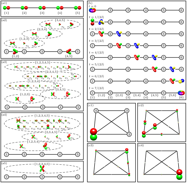
Figure 8: Visualization of experiments: In panel (a1)-(a5), the generation of five-quantum coherence in a chain consisting of five spins $1/2$ is shown for a sequence of $\pi/2$ pulses and optimized delays. The initial state is $\rho_{0}=\sum_{k=1}^{5}I_{kz}$. Panel (a1) depicts the visualization of the density matrix after an $[\pi/2]_{y}$ pulse on each spin. Panels (a2)-(a5) illustrate the state after repeated evolutions under coupling with time $t=1/(2\mathrm{J})$ followed by $[\pi/2]_{y}$ pulses on each spin, see also Fig. 3. The droplet in panel (a5) is scaled to 1/3 of its original size. Panel (b) shows the coherent transfer of the initial state $\rho_{0}=I_{1x}+iI_{1y}$ to the target state $\rho_{N}=I_{6x}+iI_{6y}$ by unitary transformations in a six-spin-$1/2$ chain: bilinear encoded states are created, which can be efficiently transferred, and they are eventually decoded at the end of the spin chain (see Ref. Khaneja and Glaser, 2002). In panels (c1)-(c4), the polarization transfer of a four-spins-$1/2$ system under isotropic mixing conditions is shown for the times (c1) 0 ms, (c2) 20 ms, (c3) 40 ms, and (c4) 133 ms, while only the linear and bilinear terms are explicitly displayed.

Table 7(b) shows the droplet functions representing the $p$-quantum operators

$$B=\prod_{k=1}^{p}I^{+}_{k}$$ (32)

with the single-spin raising operators defined as $I^{+}_{k}=I_{kx}+iI_{ky}$. In the DROPS representation, $p$-quantum operators are represented by rainbow-colored donut shapes with $p$ rainbows coding for $p$ phase transitions from 0 to $2\pi$ when the operator is rotated by 360^∘ around the $z$ axis. The color transition for an operator $I^{-}_{k}=I_{kx}-iI_{ky}$ is inverted (not shown). Again, only the coefficients of tensors with symmetry $\tau^{[N]}_{1}$ are non-zero for both $I^{+}_{k}$ and $I^{-}_{k}$ and thus, only one droplet is found.

In Tables 7(c) and (d), the droplet functions representing the antiphase operators

$$C=I_{1x}\left(\prod_{k=2}^{N}I_{kz}\right)$$ (33)

for different sizes of spin-$1/2$ systems with number of particles $N\in\{2,3,4,5,6\}$ are shown. Only coefficients of tensors with symmetries given by the partitions $\lambda(\tau_{i}^{[g]})=[N]$ and $\lambda(\tau_{i}^{[g]})=[N{-}1,1]$ are non-vanishing. There is only one symmetry type $\tau_{1}^{[N]}$ for the partition $[N]$ and the related droplet is shown in Table 7(c). The typical features of the droplet functions $f^{(G,\tau_{1}^{[N]})}$ are four arms with $N{-}2$ plates with alternating phases separating the two pairs of arms. For the partition $[N{-}1,1]$, we find $N{-}1$ different occurring symmetries $\tau_{i}^{[N]}$ with $i\in\{2,\dots,N\}$ and thus, have $N{-}1$ droplets $f^{(\ell)}$. They all have identical shapes but different sizes and one representative droplet function for this case is illustrated in Table 7(d). In total $N$ droplets visualize the antiphase operator from Eq. (33). In addition, for each tensor only orders with $|m|=\pm 1$ occur.

A.2 Visualization of experiments

We use our approach to represent and visualize experiments with up to six spins $1/2$. First we show maximum quantum coherence generation Köcher et al. (2016) in a chain of five spins $1/2$ using $\pi/2$ hard pulses and delays [see Table S2 in Ref. Köcher et al., 2016]. This is the five-spin analog to the experiment visualized given in Fig. 3 of Sec. IV for four spins. The initial state is $\rho_{0}=\sum_{k=1}^{5}I_{kz}$ and the coupling is given by an Ising Hamiltonian. All coupling constants in the drift Hamiltonian are assumed to be equal, i.e., $\mathrm{J}=\mathrm{J}_{12}=\mathrm{J}_{23}=\mathrm{J}_{34}=\mathrm{J}_{45}=\mathrm{J}$. Fig. 8(a1)-(a5) shows the droplet functions for different points in time. Panel (a1) shows the droplet functions after $\pi/2$ pulses with phases $y$ on each spin. A coupling evolution of duration $t=1/(2\mathrm{J})$ followed again by $\pi/2$ pulses with phases $y$ on all spins is repeated four times. Panels (a2)-(a5) depict the droplets representing the state after each of this sequence block. In the course of the experiment, higher orders of coherence are created, which is reflected by the occurrence of droplets of larger $g$. Although many different tensors in various subsystems and symmetries appears, the information can still be partitioned in a clear scheme. Eventually, after the experiment in panel (e), the state is fully described by a single 5-linear droplet (representing $G=\{1,\!2,\!3,\!4,\!5\}$ with the Young tableau sublabel $\tau_{1}^{[5]}$), which also contains the desired maximum-quantum coherence.

As an additional illustrative example, we present an efficient transfer of an initial state $\rho_{0}=I_{1x}+iI_{1y}$ to the target state $\rho_{t}=I_{6x}+iI_{6y}$ by unitary transformations. We consider a linear chain of six coupled spins $1/2$ and only assume Ising couplings (with identical coupling constant $\mathrm{J}$) between next neighbors and the free evolution Hamiltonian is given by $H=2\pi\sum_{k=2}^{6}\mathrm{J}\ I_{(k-1)z}I_{kz}$. The approach in Ref. Khaneja and Glaser, 2002 first encodes the initial linear operators into bilinear operators, which can then be efficiently propagated through the spin chain. Fig. 8(b) shows the state visualized by droplet functions for different points in time. The nodes represent the particles and the edges the couplings between the spins. The first row shows the visualization of $\rho_{0}$. This initial state is then encoded by applying a $\pi/2$ pulse with phase $-x$ followed by $\pi/2$ pulse with phase $y$ on the first spin, which then evolves under the the coupling Hamiltonian $H$ for a duration $1/(2\mathrm{J})$ resulting in the state shown in the second row of Fig. 8(b). Subsequently, a sequence of a $\pi/2$ pulse with phase $x$ on the first spin, a $\pi/2$ pulse with phase $y$ on the second spin and a free evolution period under the coupling Hamiltonian $H$ with duration $1/(2\mathrm{J})$ generates the encoded state, which is shown in the third row of Fig. 8(b). This encoded state, which consists only of bilinear operators can then be efficiently propagated along the spin chain by applying an effective soliton sequence composed of a $\pi/2$ pulse with phase $y$ on all spins followed by a free evolution under coupling with duration $1/(2\mathrm{J})$, which results in the propagation of the encoded state by one spin position. This is repeated three times and the resulting states are depicted in row four to six. The state is then decoded first by repeating the soliton sequence one more time (row seven) and then by a sequence consisting of a $\pi/2$ with phase $-y$ on the fifth spin, a $\pi/2$ with phase $x$ on the sixth spin, a free evolution with duration $1/(2\mathrm{J})$, and a $\pi/2$ with phase $x$ on the sixth spin is applied. This finally generates the desired state $\rho_{t}=I_{6x}+iI_{6y}$ depicted in row eight. Neglecting the durations of the hard pulses, the total transfer time is $7/(2\mathrm{J})$. For comparison,Khaneja and Glaser (2002) the same transfer could be achieved by a sequence of five next-neighbor SWAP operations (each with a duration of $3/(2\mathrm{J})$) which would require a total transfer time of $15/(2\mathrm{J})$.

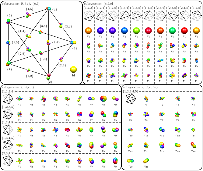
Figure 9: Visualization of a complex random matrix for five spins $1/2$. The droplet functions are arranged according to their $g$-linearity. The top left panel shows the topology of the system with nodes representing the spins and edges their couplings. Here, $f^{\text{Id}}$ is placed beneath the diagram, the droplets corresponding to $g=1$ are plotted on the nodes and the bilinear droplets for $g=2$ are placed on the edges. The top right panel illustrates $f^{(G,\tau_{i}^{[3]})}$ for all possible subsystems with $g=3$. The bottom left and right panels depict the droplet functions for all occurring subsystems with $g=4$ and $g=5$, respectively. The topologies of each $G$ are visualized by diagrams located at each subpanel. Droplet functions are normalized for better visibility.

Last, we show the visualization of the dynamics of a polarization transfer from spin one to spin two in a system consisting of four coupled spins $1/2$ under isotropic mixing conditions.Luy, Schedletzky, and Glaser (1999) Isotropic mixing is one of the most important methods to transfer polarization in high-resolution NMR spectroscopy and is frequently used in homonuclear and heteronuclear experiments to maximize polarization transfer. Its efficiency depends extremely on the mixing time duration. For four coupled spins $1/2$, the ideal isotropic mixing Hamiltonian has the form $H=2\pi\sum_{i<j}^{4}\mathrm{J}_{ij}(I_{ix}I_{jx}+I_{iy}I_{jy}+I_{iz}I_{jz})$. For the model system consisting of the ¹H nuclear spins of trans-phenylcyclopropane carboxylic acid, the coupling constants are given by $\mathrm{J}_{12}=4.1$ Hz, $\mathrm{J}_{13}=9.4$ Hz, $\mathrm{J}_{14}=6.8$ Hz, $\mathrm{J}_{23}=5.3$ Hz, $\mathrm{J}_{24}=8.2$ Hz, and $\mathrm{J}_{34}=-4.6$ Hz. Starting with the initial density density operator $\rho(0)=I_{1z}$, Fig. 8(c1)-(c4) shows the DROPS representation of the states for different mixing times: (c1) 0 ms, (c2) 20 ms, (c3) 40 ms, and (c4) 133 ms. Again, nodes represent the particles and edges their couplings. Note that for simplicity, here we only plotted the linear and bilinear tensor components. During the course of the experiment, the free evolution under isotropic mixing conditions results in the generation of coherences, which is reflected by the occurrence of non-vanishing bilinear tensors ($g=2$) and visualized by droplets located on the edges. Also small amounts of polarization occurs on the other spins depicted by the droplet functions on these nodes. After 133 ms [panel (c4)], almost all polarization has been transferred from spin one to spin two.

A.3 Representing systems consisting of five and six coupled spins $1/2$ systems

We also show the droplet functions for a (complex) random matrix $A\in\mathbb{C}^{32\times 32}$ for a five-spin-$1/2$ system. Although such systems are quite complex, with our approach, we can conveniently partition the information in different subsystems given by the panels and subpanels in Fig. 9. We find one zero-linear subsystem $G=\emptyset$ with one droplet, five linear subsystems with one droplet in each $G\in\{\{1\},\{2\},\{3\},\{4\},\{5\}\}$, and ten bilinear subsystems with also one droplet in each $G\in\{\{1,\!2\},\{1,\!3\},\{1,\!4\},\{1,\!5\},\{2,\!3\},\{2,\!4\},\{2,\!5\},\{3,\!4\},\{3,\!5\},\{4,\!5\}\}$. They can be plotted together as shown in the upper left panel of Fig. 9, where the droplets visualizing the linear subsystems are plotted on the corresponding nodes representing the spins and the droplet functions for the bilinear subsystems are placed on the edges between two spins. The identity part (Id) is placed beneath this scheme. In the upper right panel, the ten trilinear subsystems $G\in\{\{1,\!2,\!3\},\{1,\!2,\!4\},\{1,\!2,\!5\},\{1,\!3,\!4\},\{1,\!3,\!5\},\{1,\!4,\!5\},\{2,\!3,\!4\},\{2,\!3,\!5\},\{2,\!4,\!5\},\{3,\!4,\!5\}\}$, each represented by four droplets. The topology of the involved spins of each subsystem are symbolized by the sketch at the top of each subpanel. The bottom left panel shows the five four-linear subsystems with nine droplets for each $G\in\{\{1,\!2,\!3,\!4\},\{1,\!2,\!3,\!5\},\{1,\!2,\!4,\!5\},\{1,\!3,\!4,\!5\},\{2,\!3,\!4,\!5\}\}$. Again, the subsystem is graphically given at the beginning of each subpanel. Finally, the $5$-linear subsystem with 21 droplets is illustrated in the bottom right panel of Fig. 9. In total we have 122 droplet functions uniquely representing the matrix $A$. Note that we omit the superscript $[g]$ for $\tau^{[G]}$ in this figure, since $g=|G|$ holds and $G$ is clear from the context.

We conclude this section by visualizing a (complex) random matrix $A\in\mathbb{C}^{64\times 64}$ for a six coupled spins $1/2$ as given in Fig. LABEL:fig:6spin_1d2. The information can be analogously partitioned and presented as given in Fig. 9. In the upper left panel, the topology of the system is sketched. The zero-linear subsystem containing one droplet can be located beneath the scheme. The droplet functions representing the six linear subsystems $G\in\{\{1\},\{2\},\{3\},\{4\},\{5\},\{6\}\}$ are plotted on the nodes, the droplet functions of the fifteen bilinear subsystems with also one droplet in each $G\in\binom{\{1,\ldots,6\}}{2}$ are plotted on the edges. The droplet functions of the six-linear system $G=\{1,\!2,\!3,\!4,\!5,\!6\}$ are shown in the upper right panel. The panel in the center presents the twenty trilinear subsystems $G\in\binom{\{1,\ldots,6\}}{3}$ with the related droplet functions. The droplets of the 5-linear systems $G\in\binom{\{1,\ldots,6\}}{5}$ are plotted in the bottom panels of Fig. LABEL:fig:6spin_1d2. Finally, the 4-linear subsystems $G\in\binom{\{1,\ldots,6\}}{4}$ with the nine corresponding droplets for each $G$ are given in Fig. LABEL:fig:6spin_1d2_B. In total we find 423 droplets, which uniquely represents the information contained in the $64^{2}=4096$ complex matrix elements of such an operator. Again, we omit the superscript $[g]$ for $\tau$ in this figure and we use the additional ad hoc sublabels only when required, i.e., for $g=6$ and $\tau_{i}^{[6]}$ with $i\in\{7,\dots,15\}$. The standard Young tableaux for $g=5$ and $g=6$ are summarized in Table LABEL:tab:tableaux.

Appendix B Explicit values of the fractional parentage coefficients

The explicit values of the fractional parentage coefficients for up to $g=6$ are given in Tables LABEL:tab_cfp_a and LABEL:tab_cfp_a. We have used the fractional parentage coefficients as defined in Ref. Jahn and van Wieringen, 1951, and we have not applied the phase amendments from the footnote on p. 241 of Ref. Elliott, Hope, and Jahn, 1953.

References

- Feynman, Vernon, and Hellwarth (1957) R. P. Feynman, F. L. Vernon, Jr., and R. W. Hellwarth, “Geometrical Representation of the Schrödinger Equation for Solving Maser Problems,” J. Appl. Phys. 28, 49–52 (1957).
- Bernstein, King, and Zhou (2004) M. A. Bernstein, K. F. King, and X. J. Zhou, Handbook of MRI Pulse Sequences (Elsevier, Burlington-San Diego-London, 2004).
- Ernst, Bodenhausen, and Wokaun (1987) R. R. Ernst, G. Bodenhausen, and A. Wokaun, Principles of Nuclear Magnetic Resonance in One and Two Dimensions (Clarendon Press, Oxford, 1987).
- Schleich (2001) W. P. Schleich, Quantum Optics in Phase Space (Wiley-VCH, Weinheim, 2001).
- Nielsen and Chuang (2000) M. A. Nielsen and I. L. Chuang, Quantum Computation and Quantum Information (Cambridge University Press, Cambridge (UK), 2000).
- Sørensen et al. (1983) O. W. Sørensen, G. W. Eich, M. H. Levitt, G. Bodenhausen, and R. R. Ernst, “Product operator formalism for the description of nmr pulse experiments,” Progr. NMR Spectrosc. 16, 163–192 (1983).
- Donne and Gorenstein (1997) D. G. Donne and D. G. Gorenstein, “A Pictorial Representation of Product Operator Formalism: Nonclassical Vector Diagrams for Multidimensional NMR,” Concepts Magn. Reson. 9, 95–111 (1997).
- Freeman (1997) R. Freeman, A Handbook of Nuclear Magnetic Resonance, 2nd ed. (Addison Wesley Longman, Harlow, 1997).
- Curtright, Fairlie, and Zachos (2014) T. L. Curtright, D. B. Fairlie, and C. K. Zachos, A Concise Treatise on Quantum Mechanics in Phase Space (World Scientific, Singapore, 2014).
- Zachos, Fairlie, and Curtright (2005) C. K. Zachos, D. B. Fairlie, and T. L. Curtright, Quantum Mechanics in Phase Space: An Overview with Selected Papers (World Scientific, Singapore, 2005).
- Schroeck Jr. (2013) F. E. Schroeck Jr., Quantum Mechanics on Phase Space (Springer, Dordrecht, 2013).
- Wigner (1932) E. Wigner, “On the Quantum Correction For Thermodynamic Equilibrium,” Phys. Rev. 40, 749–759 (1932).
- Smithey et al. (1993a) D. T. Smithey, M. Beck, M. G. Raymer, and A. Faridani, “Measurement of the Wigner distribution and the density matrix of a light mode using optical homodyne tomography: Application to squeezed states and the vacuum,” Phys. Rev. Lett. 70, 1244–1247 (1993a).
- Smithey et al. (1993b) D. T. Smithey, M. Beck, J. Cooper, M. G. Raymer, and A. Faridani, “Complete experimental characterization of the quantum state of a light mode via the wigner function and the density matrix: application to quantum phase distributions of vacuum and squeezed-vacuum states,” Phys. Scripta 1993, 35 (1993b).
- Smithey et al. (1993c) D. T. Smithey, M. Beck, J. Cooper, and M. G. Raymer, “Measurement of number-phase uncertainty relations of optical fields,” Phys. Rev. A 48, 3159–3167 (1993c).
- Leonhardt (1997) U. Leonhardt, Measuring the Quantum State of Light (Cambridge University Press, Cambridge, 1997).
- Paris and Rehacek (2004) M. Paris and J. Rehacek, eds., Quantum State Estimation (Springer, Berlin, 2004).
- Wooters (1987) W. K. Wooters, “A Wigner-Function Formulation of Finite-State Quantum Mechanics,” Ann. Phys. 176, 1–21 (1987).
- Leonhardt (1996) U. Leonhardt, “Discrete Wigner function and quantum-state tomography,” Phys. Rev. A 53, 2998 (1996).
- Miquel, Paz, and Saraceno (2002) C. Miquel, J. P. Paz, and M. Saraceno, “Quantum computers in phase space,” Phys. Rev. A 65, 062309 (2002).
- Miquel et al. (2002) C. Miquel, J. P. Paz, M. Saraceno, E. Knill, R. Laflamme, and C. Negrevergne, “Interpretation of tomography and spectroscopy as dual forms of quantum computation,” Nature 418, 59–62 (2002).
- Gibbons, Hoffman, and Wootters (2004) K. S. Gibbons, M. J. Hoffman, and W. K. Wootters, “Discrete phase space based on finite fields,” Phys. Rev. A 70, 062101 (2004).
- Ferrie and Emerson (2009) C. Ferrie and J. Emerson, “Framed Hilbert space: hanging the quasi-probability pictures of quantum theory,” New J. Phys. 11, 063040 (2009).
- Stratonovich (1956) R. L. Stratonovich, “On distributions in Representation Space,” JETP. (U.S.S.R.) 31, 1012–1020 (1956).
- Agarwal (1981) G. S. Agarwal, “Relation between atomic coherent-state representation, state multipoles, and generalized phase-space distributions,” Phys. Rev. A 24, 2889–2896 (1981).
- Várrily and Garcia-Bondía (1989) J. C. Várrily and J. M. Garcia-Bondía, “The Moyal representation for spin,” Ann. Phys. 190, 107–148 (1989).
- Brif and Mann (1999) C. Brif and A. Mann, “Phase-space formulation of quantum mechanics and quantum-state reconstruction for physical systems with Lie-group symmetries,” Phys. Rev. A 59, 971 (1999).
- Brif and Mann (1997) C. Brif and A. Mann, “A general theory of phase-space quasiprobability distributions,” J. Phys. A: Math. Gen. 31, L9–L17 (1997).
- Heiss and Weigert (2000) S. Heiss and S. Weigert, “Discrete Moyal-type representations for a spin,” Phys. Rev. A 63, 012105 (2000).
- Klimov (2002) A. Klimov, “Exact evolution equations for quasidistribution functions,” J. Math. Phys. 43, 2202–2213 (2002).
- Klimov and Espinoza (2005) A. Klimov and P. Espinoza, “Classical evolution of quantum fluctuations in spin-like systems: squeezing and entanglement,” J. Opt. B 7, 183 (2005).
- Klimov and Espinoza (2002) A. B. Klimov and P. Espinoza, “Moyal-like form of the star product for generalized Stratonovich-Weyl symbols,” J. Phys. A 35, 8435 (2002).
- Dowling, Agarwal, and Schleich (1994) J. P. Dowling, G. S. Agarwal, and W. P. Schleich, “Wigner distribution of a general angular-momentum state: Applications to a collection of two-level atoms,” Phys. Rev. A 49, 4101–4109 (1994).
- Jessen et al. (2001) P. S. Jessen, D. L. Haycock, G. Klose, G. A. Smith, I. H. Deutsch, and G. K. Brennen, “Quantum control and information processing in optical lattices,” Quant. Inf. Computation 1, 20–32 (2001).
- Philp and Kuchel (2005) D. J. Philp and P. W. Kuchel, “A Way of Visualizing NMR Experiments on Quadrupolar Nuclei,” Concepts Magn. Reson. A 25A, 40–52 (2005).
- Harland et al. (2012) D. Harland, M. J. Everitt, K. Nemoto, T. Tilma, and T. P. Spiller, “Towards a complete and continious Wigner function for an ensemble of spins or qubits,” Phys. Rev. A 86, 062117 (2012).
- Garon, Zeier, and Glaser (2015) A. Garon, R. Zeier, and S. J. Glaser, “Visualizing operators of coupled spin systems,” Phys. Rev. A 91, 042122 (2015).
- Tilma et al. (2016) T. Tilma, M. J. Everitt, J. H. Samson, W. J. Munro, and K. Nemoto, “Wigner functions for arbitrary quantum systems,” Phys. Rev. Lett. 117, 180401 (2016).
- Koczor, Zeier, and Glaser (2016) B. Koczor, R. Zeier, and S. J. Glaser, “Time evolution of coupled spin systems in a generalized Wigner representation,” (2016), (Preprint arXiv:1612.06777v2), arXiv:1808.02697 .
- Rundle et al. (2017a) R. P. Rundle, P. W. Mills, T. Tilma, J. H. Samson, and M. J. Everitt, ‘‘Simple procedure for phase-space measurement and entanglement validation,’’ Phys. Rev. A 96, 022117 (2017a).
- Rundle et al. (2017b) R. P. Rundle, T. Tilma, J. H. Samson, V. M. Dwyer, R. F. Bishop, and M. J. Everitt, ‘‘A general approach to quantum mechanics as a statistical theory,’’ (2017b), arXiv:1708.03814v3 .
- Koczor, Zeier, and Glaser (2017) B. Koczor, R. Zeier, and S. J. Glaser, ‘‘Continuous phase-space representations for finite-dimensional quantum states and their tomography,’’ (2017), arXiv:1711.07994v2 .
- Koczor, Zeier, and Glaser (2018) B. Koczor, R. Zeier, and S. J. Glaser, ‘‘Continuous phase spaces and the time evolution of spins: star products and spin-weighted spherical harmonics,’’ (2018), arXiv:1808.02697 .
- Leiner, Zeier, and Glaser (2017) D. Leiner, R. Zeier, and S. J. Glaser, ‘‘Wigner tomography of multispin quantum states,’’ Phys. Rev. A 96, 063413 (2017).
- Leiner and Glaser (2018) D. Leiner and S. J. Glaser, ‘‘Wigner process tomography: Visualization of spin propagators and their spinor properties,’’ Phys. Rev. A 98, 012112 (2018).
- Jackson (1999) J. D. Jackson, Classical Electrodynamics, 3rd ed. (John Wiley & Sons, New York, 1999).
- James (1978) G. D. James, The Representation Theory of the Symmetric Group (Springer, Berlin, 1978).
- James and Kerber (1981) G. James and A. Kerber, The Representation Theory of the Symmetric Group (Addison-Wesley, Reading, MA, 1981).
- Ceccherini-Silberstein, Scarabotti, and Tolli (2010) T. Ceccherini-Silberstein, F. Scarabotti, and F. Tolli, Representation Theory of the Symmetric Groups (Cambridge University Press, Cambridge, 2010).
- Boerner (1967) H. Boerner, Darstellungen von Gruppen, 2nd ed. (Springer, Berlin, 1967).
- Hamermesh (1962) M. Hamermesh, Group Theory (Addison-Wesley, Reading, MA, 1962).
- Sagan (2001) B. E. Sagan, The Symmetric Group, 2nd ed. (Springer, New York, 2001).
- Tung (1985) W. K. Tung, Group Theory in Physics (World Scientific Publishing Company, Incorporated, 1985).
- Racah (1965) G. Racah, ‘‘Group Theory and Spectroscopy,’’ in Ergebnisse der exakten Naturwissenschaften, 37. Band (Springer, Berlin, 1965) pp. 28--84.
- Elliott and Lane (1957) J. P. Elliott and A. M. Lane, ‘‘The Nuclear Shell-Model,’’ in Encyclopedia of Physics, Volume XXXIX, Structure of Atomic Nuclei (Springer, Berlin, 1957) pp. 241--410.
- Kaplan (1975) I. G. Kaplan, Symmetry of Many-Electron Systems (Academic Press, New York, 1975).
- Silver (1976) B. L. Silver, Irreducible Tensor Methods (Academic Press, New York, 1976).
- Chisholm (1976) C. D. H. Chisholm, Group Theoretical Techniques in Quantum Chemistry (Academic Press, London, 1976).
- Kramer, John, and Schenzle (1981) P. Kramer, G. John, and D. Schenzle, Group Theory and the Interaction of Composite Nucleon Systems (Vieweg, Braunschweig, 1981).
- Jahn and van Wieringen (1951) H. A. Jahn and H. van Wieringen, ‘‘Theoretical studies in nuclear structure IV. Wave functions for the nuclear -shell Part A. fractional parentage coefficients,’’ Proc. R. Soc. Lond. A 209, 502--524 (1951).
- Weyl (1927) H. Weyl, ‘‘Quantenmechanik und Gruppentheorie,’’ Z. Phys. 46, 1--33 (1927).
- Weyl (1931) H. Weyl, Gruppentheorie und Quantenmechanik, 2nd ed. (Hirzel, Leipzig, 1931) english translation in Weyl (1950).
- Weyl (1950) H. Weyl, The Theory of Groups & Quantum Mechanics, 2nd ed. (Dover Publ., New York, 1950).
- Weyl (1953) H. Weyl, The Classical Groups: Their Invariants and Representations, 2nd ed. (Princeton University Press, Princeton, 1953).
- Wigner (1931) E. Wigner, Gruppentheorie und ihre Anwendung auf die Quantenmechanik der Atomspektren (Friedrich Vieweg & Sohn, Braunschweig, 1931) (English translation in Wigner (1959)).
- Wigner (1959) E. P. Wigner, Group Theory and its Application to the Quantum Mechanics of Atomic Spectra (Academic Press, London, 1959).
- Condon and Shortley (1935) E. U. Condon and G. H. Shortley, The Theory of Atomic Spectra (Cambridge University Press, Cambridge, 1935).
- Racah (1941) G. Racah, ‘‘Theory of Complex Spectra I,’’ Phys. Rev. 61, 186--197 (1941).
- Racah (1942) G. Racah, ‘‘Theory of Complex Spectra II,’’ Phys. Rev. 62, 438--462 (1942).
- Racah (1943) G. Racah, ‘‘Theory of Complex Spectra III,’’ Phys. Rev. 63, 367--382 (1943).
- Racah (1949) G. Racah, ‘‘Theory of Complex Spectra IV,’’ Phys. Rev. 76, 1353--1365 (1949).
- Fano and Racah (1959) U. Fano and G. Racah, Irreducible Tensorial Sets (Academic Press, New York, 1959).
- Edmonds (1960) A. R. Edmonds, Angular momentum in quantum mechanics (Princeton University Press, Princeton, 1960).
- Griffith (2006) J. S. Griffith, The Irreducible Tensor Method for Molecular Symmetry Groups (Dover Publications, Mineola, NY, 2006).
- Judd (1998) B. R. Judd, Operator Techniques in Atomic Spectroscopy (Princeton University Press, Princeton, 1998).
- Miller (1972) W. Miller, Symmetry Groups and Their Applications, Pure and Applied Mathematics (Academic Press, London, 1972).
- Ludwig and Falter (1996) W. Ludwig and C. Falter, Symmetries in Physics, 2nd ed. (Springer, Berlin, 1996).
- Slater (1960) J. C. Slater, Quantum Theory of Atomic Structure, Vol. II (McGraw-Hill, New York, 1960).
- de-Shalit and Talmi (1963) A. de-Shalit and I. Talmi, Nuclear Shell Theory (Academic Press, New York, 1963).
- Pauncz (1967) R. Pauncz, Alternant Molecular Orbital Method (W. B. Saunders Company, Philadelphia, 1967).
- Wybourne (1970) B. G. Wybourne, Symmetry Principles and Atomic Spectroscopy (Wiley-Interscience, New York, 1970).
- Elliott and Dawber (1979) J. P. Elliott and P. G. Dawber, Symmetry in Physics, 2 Volumes (Macmillan, Hampshire, 1979).
- Condon and Odabaşi (1980) E. U. Condon and H. Odabaşi, Atomic Structure (Cambridge University Press, Cambridge, 1980).
- Rudzikas (1997) Z. Rudzikas, Theoretical Atomic Spectroscopy (Cambrdige University Press, Cambridge, 1997).
- Chaichian and Hagedorn (1998) M. Chaichian and R. Hagedorn, Symmetries in Quantum Mechanics: From Angular Momentum to Supersymmetry (Institute of Physics, Bristol, 1998).
- Rowe and Wood (2010) D. J. Rowe and J. L. Wood, Fundamentals of Nuclear Models: Foundational Models (World Scientific Publ., Singapore, 2010).
- Listerud (1987) J. Listerud, Techniques in Solid State NMR, Ph.D. thesis, University of Washington (1987).
- Listerud, Glaser, and Drobny (1993) J. Listerud, S. J. Glaser, and G. P. Drobny, ‘‘Symmetry and Isotropic Coherence Transfer. II. Three Spin Calculations Using a Young Tableaux Formulation,’’ Mol. Phys. 78, 629--658 (1993).
- Biedenharn and Louck (1981) L. C. Biedenharn and J. D. Louck, Angular Momentum in Quantum Physics (Addison-Wesley, Reading, MA, 1981).
- Note (1) Spherical harmonics (and droplet functions) are plotted throughout this work by mapping their spherical coordinates and to the radial part and phase .
- Judd et al. (1974) B. R. Judd, W. Miller, Jr., J. Patera, and P. Winternitz, ‘‘Complete sets of commuting operators and scalars in the enveloping algebra of ,’’ J. Math. Phys. 15, 1787--1799 (1974).
- Sharp (1975) R. T. Sharp, ‘‘Internal-labeling operators,’’ J. Math. Phys. 16, 2050--2053 (1975).
- Iachello and Levine (1995) F. Iachello and R. D. Levine, Algebraic Theory of Molecules (Oxford University Press, New York, 1995).
- Merzbacher (1998) E. Merzbacher, Quantum Mechanics, 3rd ed. (John Wiley & Sons, New York, 1998).
- Pauncz (1995) R. Pauncz, The Symmetric Group in Quantum Chemistry (CRC Press, Boca Raton, 1995).
- Feenberg and Phillips (1937) E. Feenberg and M. Phillips, ‘‘On the Structure of Light Nuclei,’’ Phys. Rev. 51, 597--608 (1937).
- Zare (1988) R. N. Zare, Angular Momentum (John Wiley & Sons, New York, 1988).
- Beringer, J. et al. (2012) (Particle Data Group) Beringer, J. et al. (Particle Data Group), ‘‘The Review of Particle Physics,’’ Phys. Rev. D 86, 010001 (2012).
- Sanctuary and Temme (1985) B. C. Sanctuary and F. P. Temme, ‘‘Multipole N.M.R. XIII. multispin interactions and symmetry in Liouville space,’’ Mol. Phys. 55, 1049--1062 (1985).
- Fano (1953) U. Fano, ‘‘Geometrical characterization of nuclear states and the theory of angular correlations,’’ Phys. Rev. 90, 577--579 (1953).
- Messiah (1962) A. Messiah, Quantum mechanics, Vol. II (North-Holland, Amsterdam, 1962).
- Landau and Lifshitz (1977) L. D. Landau and E. M. Lifshitz, Quantum mechanics, Vol. 3 (Pergamon Press, Oxford, 1977).
- Dür, Vidal, and Cirac (2000) W. Dür, G. Vidal, and J. I. Cirac, ‘‘Three qubits can be entangled in two inequivalent ways,’’ Phys. Rev. A 62, 062314 (2000).
- Briegel and Raussendorf (2001) H. J. Briegel and R. Raussendorf, ‘‘Persistent Entanglement in Arrays of Interacting Particles,’’ Phys. Rev. Lett. 86, 910--913 (2001).
- Verstraete et al. (2002) F. Verstraete, J. Dehaene, B. De Moor, and H. Verschelde, ‘‘Four qubits can be entangled in nine different ways,’’ Phys. Rev. A 65, 052112 (2002).
- Dicke (1954) R. H. Dicke, ‘‘Coherence in spontaneous radiation processes,’’ Phys. Rev. 93, 99--110 (1954).
- Stockton et al. (2003) J. K. Stockton, J. M. Geremia, A. C. Doherty, and H. Mabuchi, ‘‘Characterizing the entanglement of symmetric many-particle spin- systems,’’ Phys. Rev. A 67, 022112 (2003).
- Köcher et al. (2016) S. Köcher, T. Heydenreich, Y. Zhang, G. N. Reddy, S. Caldarelli, H. Yuan, and S. J. Glaser, ‘‘Time-optimal excitation of maximum quantum coherence: Physical limits and pulse sequences,’’ J. Chem. Phys. 144, 164103 (2016).
- Note (2) Hermitian operators lead to positive and negative values, which are shown in red (dark gray) and green (light gray).
- Glaser et al. (2015) S. J. Glaser, U. Boscain, T. Calarco, C. P. Koch, W. Köckenberger, R. Kosloff, I. Kuprov, B. Luy, S. Schirmer, T. Schulte-Herbüggen, D. Sugny, and F. K. Wilhelm, ‘‘Training Schrödinger’s Cat: Quantum Optimal Control,’’ Eur. Phys. J. D 69, 279 (2015).
- Glaser, Tesch, and Glaser (2015) N. J. Glaser, M. Tesch, and S. J. Glaser, ‘‘SpinDrops (Version 1.2.2) [Mobile application],’’ (2015), itunes.apple.com.
- Tesch, Glaser, and Glaser (2018) M. Tesch, N. J. Glaser, and S. J. Glaser, ‘‘Spindrops 2.0,’’ (2018), https://spindrops.org.
- Luy and Glaser (2000) B. Luy and S. J. Glaser, ‘‘Negative polarization transfer between a spin 1/2 and a spin 1,’’ Chem. Phys. Lett. 323, 377--381 (2000).
- Horn and Johnson (1991) R. A. Horn and C. R. Johnson, Topics in Matrix Analysis (Cambridge University Press, Cambridge, 1991).
- Henderson and Searle (1981) H. V. Henderson and S. R. Searle, ‘‘The Vec-Permutation Matrix, the Vec Operator, and Kronecker Products: A Review,’’ Lin. Multilin. Alg. 9, 271--288 (1981).
- Fuhrmann (2012) P. A. Fuhrmann, A Polynomial Approach to Linear Algebra, 2nd ed. (Springer, New York, 2012).
- (117) J. Huizenga, ‘‘Necessary and sufficient conditions for a sum of idempotents to be idempotent,’’ MathOverflow, https://mathoverflow.net/q/115255 (2012-12-03).
- Simon (1995) B. Simon, Representations of Finite and Compact Groups (Oxford University Press, Oxford, 1995).
- Keppeler and Sjödahl (2014) S. Keppeler and M. Sjödahl, ‘‘Hermitian Young operators,’’ J. Math. Phys. 55, 021702 (2014).
- Alcock-Zeilinger and Weigert (2017a) J. Alcock-Zeilinger and H. Weigert, ‘‘Compact Hermitian Young projection operators,’’ J. Math. Phys. 58, 051702 (2017a).
- Alcock-Zeilinger and Weigert (2017b) J. Alcock-Zeilinger and H. Weigert, ‘‘Transition operators,’’ J. Math. Phys. 58, 051703 (2017b).
- Stembridge (2011) J. R. Stembridge, ‘‘Orthogonal sets of Young symmetrizers,’’ Adv. Appl. Math. 46, 576--582 (2011).
- Acin et al. (2018) A. Acin, I. Bloch, H. Buhrman, T. Calarco, C. Eichler, J. Eisert, D. Esteve, N. Gisin, S. J. Glaser, F. Jelezko, S. Kuhr, M. Lewenstein, M. F. Riedel, P. O. Schmidt, R. Thew, A. Wallraff, I. Walmsley, and F. K. Wilhelm, ‘‘The quantum technologies roadmap: a European community view,’’ New J. Phys. 20, 080201 (2018).
- Bosma, Cannon, and Playoust (1997) W. Bosma, J. J. Cannon, and C. Playoust, ‘‘The MAGMA Algebra System I: The User Language,’’ J. Symbolic Comput. 24, 235--265 (1997).
- The MathWorks Inc. (2017) The MathWorks Inc., MATLAB, version 9.2 (R2017a), Natick, Massachusetts (2017).
- The Sage Developers (2018) The Sage Developers, SageMath, the Sage Mathematics Software System (Version 8.3) (2018), http://www.sagemath.org.
- Khaneja and Glaser (2002) N. Khaneja and S. J. Glaser, ‘‘Efficient Transfer of Coherence through Ising Spin Chains,’’ Phys. Rev. A 66, 060301(R) (2002).
- Luy, Schedletzky, and Glaser (1999) B. Luy, O. Schedletzky, and S. J. Glaser, ‘‘Analytical polarization transfer functions for four coupled spins 1/2 under isotropic mixing conditions,’’ J. Magn. Reson. 138, 19--27 (1999).
- Elliott, Hope, and Jahn (1953) J. P. Elliott, J. Hope, and H. A. Jahn, ‘‘Theoretical studies in nuclear structure IV. Wave functions for the nuclear -shell Part B. fractional parentage coefficients,’’ Philos. Trans. Royal Soc. A 246, 241--279 (1953).