Phenomenological model for the gravitational-wave signal from precessing binary black holes with two-spin effects

Abstract

The properties of compact binaries, such as masses and spins, are imprinted in the gravitational-waves they emit and can be measured using parameterised waveform models. Accurately and efficiently describing the complicated precessional dynamics of the various angular momenta of the system in these waveform models is the object of active investigation. One of the key models extensively used in the analysis of LIGO and Virgo data is the single-precessing-spin waveform model IMRPhenomPv2. In this article we present a new model IMRPhenomPv3 which includes the effects of two independent spins in the precession dynamics. Whereas IMRPhenomPv2 utilizes a single-spin frequency-dependent post-Newtonian rotation to describe precession effects, the improved model, IMRPhenomPv3, employs a double-spin rotation that is based on recent developments in the description of precessional dynamics. Besides double-spin precession, the improved model benefits from a more accurate description of precessional effects. We validate our new model against a large set of precessing numerical-relativity simulations. We find that IMRPhenomPv3 has better agreement with the inspiral portion of precessing binary-black-hole simulations and is more robust across a larger region of the parameter space than IMRPhenomPv2. As a first application we analyse, for the first time, the gravitational-wave event GW151226 with a waveform model that describes two-spin precession. Within statistical uncertainty our results are consistent with published results. IMRPhenomPv3 will allow studies of the measurability of individual spins of binary black holes using GWs and can be used as a foundation upon which to build further improvements, such as modeling precession through merger, extending to higher multipoles, and including tidal effects.

I Introduction

Binary systems of compact bodies such as neutron stars and black holes generate gravitational waves that are detectable by second-generation ground based interferometers. The energy carried away by GWs causes the orbit to decay and the binary to merge on astrophysical time scales. These tiny ripples in spacetime propagate almost completely unaffected through the Universe and have the source properties imprinted in the gravitational waveform. In August 2017 the second observing run (O2) of the detectors aLIGO Aasi et al. (2015) and Virgo Acernese et al. (2015) ended, and to date O1 and O2 have resulted in the publication of 6 likely binary black hole (BBH) Abbott et al. (2016a) (LIGO and Virgo Scientific Collaboration); Abbott et al. (2016b) (LIGO and Virgo Scientific Collaboration); Abbott et al. (2017) (LIGO and Virgo Scientific Collaboration); Abbott et al. (2017a, b) merger events, and the joint GW-electromagnetic observation of a pair of merging NSs Abbott et al. (2017c, d).

Detection and characterisation of GW signals is carried out by a suite of software pipelines that analyse detector data using a variety of analysis methods Messick et al. (2017); Dal Canton et al. (2014); Usman et al. (2016); Nitz et al. (2017); Klimenko et al. (2016). Matched-filter-based analyses, used in the search for and parameter estimation Cutler and Flanagan (1994); Veitch et al. (2015); Abbott et al. (2016a) of GW signals from compact binaries require accurate and computationally-inexpensive models for the GW signals, which are used as templates. The need for computationally tractable analyses is best satisfied by frequency-domain models. Moreover, the accuracy of GW signal models and the quantity and quality of the physical effects they include impact both the types of sources GW analyses are sensitive to and the fidelity of the conclusions we draw about their properties.

One such physical effect that has been at the center of waveform-modeling efforts in the recent years is spin-precession: when the binary components’ spin angular momenta are misaligned with the orbital angular momentum of the binary, spin-orbit and spin-spin interactions cause the binary orbit to change orientation in space, resulting in modulations in the observed signal amplitude and phase Apostolatos et al. (1994); Kidder (1995). Modeling these modulations is a challenging task, especially for systems with unequal-mass components that are observed from close to the binary plane, since this case requires accurate modeling of both spin-precession effects and higher modes beyond the dominant $(\ell,|m|)=(2,2)$ multipoles.

Numerous models have been developed in the recent years with the goal of providing a complete coverage across the BBH parameter space containing all relavent physical effects required for the current sensitivity of GW detectors.

The effective-one-body–numerical-relativity (EOB-NR) model, SEOBNRv3 Pan et al. (2014), built upon the non-precessing model of Taracchini et al. (2014), is a time-domain two-spin precessing model. It provides the $(\ell,|m|)\in((2,2),(2,1))$ multipoles in the co-precessing frame although only the $(2,2)$ is calibrated to numerical relativity (NR) data. This model has been shown to accurately model the $\ell=2$ multipoles from precessing BBHs Babak et al. (2017), however, as it requires the integration of a set of coupled ordinary differential equations it incurs a large computational cost.

The phenomenological (phenom) waveform models are typically developed and constructed in the frequency-domain and the precessing model IMRPhenomP was presented in Hannam et al. (2014). IMRPhenomP is built upon the non-precessing model of Santamaría et al. (2010) was later upgraded to IMRPhenomPv2 which used the non-precessing model of Husa et al. (2016); Khan et al. (2016). Despite its computational efficiency IMRPhenomP is limited to single-spin effects, though this choice was shown to not lead to appreciable biases in the characterization of the first BBH signal Abbott et al. (2016b, 2017e). A time-domain phenom model for precessing BBHs was presented in Sturani et al. (2010), however, it is restricted to equal-mass BBHs with spin magnitudes up to $0.6$.

Recently work has been done to develop models for multipoles beyond the dominant $(\ell,|m|)=(2,2)$ multipole. The first of such models were the non-spinning EOB-NR model of Pan et al. (2011) and a non-spinning phenom model was presented in Mehta et al. (2017). The first extension of these higher multipole modes into spinning non-precessing BBHs has been acomplished both by the phenom London et al. (2018) and Effective-One-Body (EOB) Cotesta et al. (2018) approaches.

An alternative approach to waveform modeling has been successful in building surrogate models Field et al. (2014) that interpolate GW data from NR simulations. The surrogate model of Blackman et al. (2017) is a fully precessing, time-domain model containing $\ell\leqslant 4$ multipoles, however, it is restricted to systems where the ratio of the components’ masses is less than two.

In this paper we take another step towards a computationally-tractable GW model that accurately models generic BBH systems by introducing the frequency-domain fully-precessing phenomenological model, IMRPhenomPv3, that describes the inspiral, merger, and ringdown phases of spinning BBHs. Our upgrade from IMRPhenomPv2 to IMRPhenomPv3 hinges on a novel closed-form solution to the differential equations that describe precession including the effects of radiation reaction in the Post Newtonian (PN) regime where the binary components are well-separated Chatziioannou et al. (2017a, b). This closed-form solution to the precession equations including the effects of radiation reaction has been shown to accurately describe precession for systems with generic masses and spins Chatziioannou et al. (2017a). Moreover, since it is an analytic frequency-domain model, it is also amenable to the reduced-order-quadrature method to greatly accelerate likelihood evaluations for fast parameter estimation Smith et al. (2016). In addition, IMRPhenomPv2 exhibits non-physical precession behaviour for some high mass-ratio, anti-aligned spin configurations, as discussed in Sec. II.4, but this behaviour is not observed in in IMRPhenomPv3.

We validate our new model by comparing against a large set of precessing NR waveforms. We find that the improved treatment of the inspiral improves the accuracy of the model for measurement of low-mass systems in LIGO-Virgo data. Finally, as a first application and demonstration of our model’s readiness we perform a Bayesian parameter estimation analysis (using LALInference Veitch et al. (2015)) on the GW event GW151226 Abbott et al. (2016b) (LIGO and Virgo Scientific Collaboration). This is a $\sim$22$\,M_{\odot}$ BBH signal where at least one of the BHs is measured to have a dimensionless spin magnitude of $\gtrsim 0.2$ at the 99% credible level. The presence of spin and the low total mass, which implies a large number of GW cycles ($\sim$55) measurable by the detector, makes this an ideal candidate to look for evidence of precession. This is the first analysis of GW151226 with a Inspiral-Merger-Ringdown (IMR) precession model with the full 4 degrees of freedom coming from precession.

II Building the new model

In this section we describe the construction of IMRPhenomPv3 and highlight the improvements compared to IMRPhenomPv2.

II.1 Precessing BBH phenomenology

A quasicircular BBH system can be parameterised by only 7 intrinsic parameters; the mass-ratio $q=m_{1}/m_{2}$ and 6 spin angular momenta $\vec{S}_{1}$ and $\vec{S}_{2}$. In addition, the total mass $M=m_{1}+m_{2}$ can be factored out and systems with different total masses can be obtained with appropriate scaling of $M$. For each BBH we can define a Newtonian orbital angular momentum $\vec{L}$, which is perpendicular to the instantaneous orbital plane and a total angular momentum $\vec{J}=\vec{L}+\vec{S}_{1}+\vec{S}_{2}$.

We classify BBH systems into different categories according to their spin. Non-precessing systems have BH spins that are either aligned- or anti-aligned with $\vec{L}$. Systems with spins (anti-)aligned with $\vec{L}$ plunge and merge at (larger) smaller separations compared to nonspinning binaries, shifting the merger and ringdown part of the signal to (lower) higher GW frequencies. Precessing BBH are systems with arbitrary BH spin orientation. Interactions between the BH spins and $\vec{L}$ introduce a torque on the orbital angular momentum causing it to precess around the (almost constant) direction of the total angular momentum. Special sub-categories of precessing systems include simple- and transitional- precession binaries Apostolatos et al. (1994); Kidder (1995). Most binaries undergo simple precession, while transitional precession occurs when $\vec{J}=\vec{L}+\vec{S}_{1}+\vec{S}_{2}\approx 0$ Apostolatos et al. (1994).

II.2 Modeling precessing BBHs

The complicated phenomenology of generically precessing BBHs makes waveform modeling especially challenging. A significant advance was achieved when it was observed that the GW signal from precessing binaries is simplified when observed in a frame that is adapted to the precessional motion of the binary Schmidt et al. (2011); O’Shaughnessy et al. (2011). In this non-inertial (co-precessing) frame the $z$-axis approximately tracks the orientation of the orbital plane. When the waveform is transformed into this frame it closely mimics the signal of the equivalent BBH system that has the spin components perpendicular to $\vec{L}$ set to zero Schmidt et al. (2011); Pekowsky et al. (2013). This is a consequence of the approximate decoupling between the components of spin parallel and perpendicular to $\vec{L}$; the former influences the rate of inspiral and the latter drives the precessional motion Apostolatos et al. (1994); Schmidt et al. (2011); Buonanno et al. (2003).

This observation led to a method for building models for the gravitational waveform from generic precessing BBHs by first constructing a model for the gravitational waveform produced by the equivalent non-precessing BBHs and then introducing precession through a time (or frequency) dependent rotation of the signal derived from the orbital dynamics Schmidt et al. (2012). Colloquially this procedure is denoted “twisting-up” a non-precessing model to produce a precessing model Schmidt et al. (2012).

Beginning with an inertial frame that is aligned with the total angular momentum at some reference frequency $\hat{z}=\hat{J}$ we describe the orbital angular momentum by the azimuthal and polar angles ($\alpha$, $\beta$). In order to completely specify the rotation we use the frame that minimises precessional effects and adopt the “minimum rotation condition” Boyle et al. (2011) which enforces the third Euler angle to obey $\dot{\epsilon}(t)=\dot{\alpha}(t)\,{\rm{cos}}(\beta(t))$. This angle constitutes a modification to the orbital phase chosen so that the frequency in the inertial frame is the same as the frequency in the co-precessing frame. For a geometric depiction, see Figure 1 in Ref. Chatziioannou et al. (2017a).

This procedure was used to produce the first precessing IMR models Hannam et al. (2014); Taracchini et al. (2014); Pan et al. (2014). The general procedure is as follows. First we express the two GW polarisations $h_{+}$ and $h_{\times}$ as a linear combination of spherical harmonics with spin-weight $-2$. The coefficients of the basis functions are the GW multipoles $h_{\ell,m}$, see equation (1). This decomposition is performed in a frame that is aligned with the total angular momentum and the direction of propagation is given by the spherical polar coordinates ($\theta,\varphi$),

$$h(t;\theta,\phi)=h_{+}\,-\,ih_{\times}=\sum_{\ell\geqslant 2,m}h_{\ell,m}(t)Y_{\ell,m}^{-2}(\theta,\varphi).$$ (1)

From here we wish to express the GW multipoles from precessing BBHs $h^{prec}_{\ell,m}$ in terms of the multipoles from non-precessing BBHs $h^{\begin{subarray}{c}non-\\ prec\end{subarray}}_{\ell,m}$ and the appropriate angles that describe the “twisting-up” from non-precessional to precessional dynamics. This is done by applying the Wigner-D rotation matrices to the GW multipoles from the non-precessing system using the angles $(\alpha,\beta,\epsilon)$ Schmidt et al. (2011); O’Shaughnessy et al. (2011); Boyle et al. (2011); Schmidt et al. (2012). Here we focus on the $\ell=2$ multipoles and the case where the non-precessing model only contains the $\ell=|m|=2$ multipoles. In that case, the waveform is given by

$$h^{prec}_{2,m}(t)=e^{-im\alpha(t)}\sum_{|m^{\prime}|=2}e^{im^{\prime}\epsilon(t)}\,d^{2}_{m^{\prime},m}(-\beta(t))\,h^{\begin{subarray}{c}non-\\ prec\end{subarray}}_{2,m^{\prime}}(t)\,.$$ (2)

In order to complete the tranformation from a non-precessing IMR model to a precessing IMR model we also need to modify the mapping between the inspiraling progenitor BHs and the final BH, taking into account the effect of precession. We typically assume that changes in the GW flux due to precession can be neglected so that the estimate of the final mass can be taken from fits to NR simulations of non-precessing systems. The final spin, however, is sensitive to precession and therefore needs to be modified from the model used in the underlying non-precessing model.

In the next sections, we review the angles $(\alpha_{\rm{v2}},\beta_{\rm{v2}},\epsilon_{\rm{v2}})$ that were used for the IMRPhenomPv2 model and then we describe the updated $(\alpha_{\rm{v3}},\beta_{\rm{v3}},\epsilon_{\rm{v3}})$ that we employ to produce the updated model IMRPhenomPv3.

II.3 Review of IMRPhenomPv2

The method described in the previous section to construct a complete IMR model for precessing BBHs was used to create the IMRPhenomP model Hannam et al. (2014). The original model used the IMRPhenomC Santamaría et al. (2010) model to describe the non-precessing system, but was subsequently enhanced to IMRPhenomPv2, which uses IMRPhenomD Husa et al. (2016); Khan et al. (2016), a more accurate aligned-spin model valid for larger mass-ratio binaries and BHs with larger spin magnitudes. Moreover IMRPhenomD includes some two-spin information during the inspiral. Both of these underlying aligned-spin models provide only the $\ell=|m|=2$ spherical harmonic multipole.

In both previous versions of IMRPhenomP the precession angles $(\alpha_{\rm{v2}},\beta_{\rm{v2}},\epsilon_{\rm{v2}})$ were computed by a closed-form frequency-domain expression derived under the assumption of a single-spin system and parameterised by the aligned effective-spin parameter $\chi_{\rm{eff}}$ and the precession effective-spin parameter $\chi_{p}$ Schmidt et al. (2015) defined as

$$\chi_{p}:=\frac{\max\left(A_{1}S_{1\bot},A_{2}S_{2\bot}\right)}{A_{1}m_{1}^{2}}\,,$$ (3)

where $A_{1}=2+\frac{3m_{2}}{2m_{1}}$, $A_{2}=2+\frac{3m_{1}}{2m_{2}}$ and $S_{i\bot}$ are the magnitudes of the spin-angular momenta perpendicular to $\vec{L}$. Additionally, IMRPhenomP used a small-angle approximation for the opening angle ($\beta$), an assumption that was subsequently relaxed in IMRPhenomPv2.

The expressions for $(\alpha_{\rm{v2}},\beta_{\rm{v2}},\epsilon_{\rm{v2}})$ were derived under the stationary phase approximation (SPA) Droz et al. (1999) and are used to “twist-up” the entire waveform, including through merger and ringdown, where the assumptions of SPA are formally invalid. Nevertheless the extrapolation of the PN expressions into the merger and ringdown have been shown to not impair the model, so long as the mass-ratio and spin are not large, see Hannam et al. (2014) and Section III.

IMRPhenomPv2 uses a single-spin approximation that only models the simple-precession case where the direction of $J$ is relatively constant during the inspiral, and the direction of the final BH spin is assumed to be parallel to $J$. The magnitude of the final spin angular momentum $S_{f}$ is computed as the sum of parallel and perpendicular angular momentum components with respect to $\vec{L}$. $S_{\begin{subarray}{c}non-\\ prec\end{subarray}}$ is the angular momentum from the non-precessing system and $S_{\bot}$ is the angular momentum of the in-plane spin components.

$$S_{f}\equiv M_{f}^{2}\chi_{f}=\sqrt{S^{2}_{\bot}+S^{2}_{\begin{subarray}{c}non-\\ prec\end{subarray}}}\,.$$ (4)

The final dimensionless spin magnitude $\chi_{f}$, with a free parameter $\lambda$ is written as pv (2); Jiménez-Forteza et al. (2017)

$$\chi_{f}=\sqrt{\left(S_{\bot}\frac{\lambda^{2}}{M_{f}^{2}}\right)^{2}+\chi^{2}_{\begin{subarray}{c}non-\\ prec\end{subarray}}}\,.$$ (5)

The choice made for $\lambda$ in IMRPhenomPv2 is $\lambda=M_{f}/M$ implies that the $S_{\bot}$ angular momentum gets scaled by the initial total mass. We comment that this is a fairly arbitrary choice as we have a model for $M_{f}$ that we use in the non-precessing part Husa et al. (2016). However, it was found that this simplification still yielded a model with acceptable accuracy. Finally, $S_{\bot}$ is approximated using the effective precessing parameter $\chi_{p}$ and computing the angular momentum by assuming only the primary BH has in-plane spin components i.e.

$$S_{\bot}=m_{1}^{2}\chi_{p}\,.$$ (6)

The model IMRPhenomPv2 has been used in numerous publications to estimate the source parameters of all BBH observations in the LIGO-Virgo O1 and O2 runs, eg. Abbott et al. (2016c, d, e); Abbott et al. (2016b) (LIGO and Virgo Scientific Collaboration); Abbott et al. (2016f); Abbott et al. (2017) (LIGO and Virgo Scientific Collaboration); Abbott et al. (2017a, b) and has been the basis of a ROQ approximation to the likelihood Smith et al. (2016) that has enabled fast parameter estimation of GW sources Vitale et al. (2017). The model’s low computational cost has also enabled it to form the basis of the model IMRPhenomPv2_NRTidal Dietrich et al. (2018) used for the analysis of the long BNS signal GW170817 Abbott et al. (2018a, b).

II.4 Issues with IMRPhenomPv2 precession angles

Despite IMRPhenomPv2’s good performance across the parameter space, there are some known issues with the precession angles. Specifically, the angle $\alpha_{\rm{v2}}(f)$ is written as a power series in $f$, including terms up to next-to-next-to-leading order (3PN) in the spin. The leading-order Newtonian term (see, for example, Ref. Apostolatos et al. (1994)) is

$$\alpha_{\rm{v2}}^{N}=\alpha_{0}-\frac{20\left(1+\frac{3}{4q}\right)}{192f},$$ (7)

where $\alpha_{0}$ is a constant. At this order, the precession angle is a monotonically increasing function, which is what we expect in a physical system exhibiting simple precession: the orbital angular momentum vector precesses around the total angular momentum throughout the binary’s evolution, and the rate of precession steadily increases. At leading order Apostolatos et al. (1994) we also see that the precession angle (and therefore also the precession frequency) depend only on the mass-ratio of the binary; the spin affects the precession rate at higher orders.

If we extend this expression up to $f^{1/3}$, as is done in the NNLO expressions used in IMRPhenomPv2 Schmidt (which also include a $\log(f)$ term), then higher order terms can enter with opposing signs. In some cases this can remove the monotonicity of $\alpha_{\rm{v2}}(f)$, even for simple-precession configurations where we know that such behavior is not physically consistent.

Figure 1 show examples of this behavior. We first consider a configuration that is comparable to those already found in GW observations: the mass ratio is 1, the component of the spin parallel to the orbital angular momentum is zero, i.e., $\chi_{\rm eff}=0$, and the larger BH has a spin of magnitude 0.9 lying in the orbital plane, i.e., $\chi_{p}=0.9$; since $\chi_{p}$ has not been constrained in observations to date, a value of $0.9$ is consistent with the measured parameters. The angle of the spin in the plane at a particular reference frequency determines the constant $\alpha_{0}$, but we will focus here on the frequency evolution of the precession angle. We plot the precession angle $\alpha_{\rm{v2}}(f)-\alpha(f_{0})$, where $Mf_{0}=0.0001$, which corresponds to approximately 2 Hz for a binary with a total mass of 10 $M_{\odot}$. The results are shown up to the Schwarzschild ISCO frequency ($Mf=0.0217$). We can see that $\alpha_{\rm{v2}}(f)$, as predicted by the leading-order Eq. 7 (blue dashed line), the full NNLO expressions used for IMRPhenomPv2 (blue solid line), the full IMRPhenomPv3 expression (orange dashed line), and the trunchated IMRPhenomPv3 expression (orange solid line) all agree well, even though spin effects are not included in the leading-order result.

In the second example, we can see that the NNLO expression is needed to accurately describe the precession for higher mass ratios and higher spins. This example shows $\alpha_{\rm{v2}}(f)-\alpha(f_{0})$ for a binary with mass-ratio 8, again $\chi_{\rm eff}=0$ and $\chi_{p}=0.9$. The NNLO IMRPhenomPv2 and the IMRPhenomPv3 expressions agree well, but the leading-order expression accumulates a difference against the others of $\sim$60 rad, or $\sim$10 precession cycles, out of $\sim$47 cycles over the course of the entire inspiral. This level of agreement between the IMRPhenomPv2 and IMRPhenomPv3 expressions is typical across all configurations with mass ratios up to $\sim$5, so we can be confident that IMRPhenomPv2 accurately models the precession angle $\alpha_{\rm{v2}}$ with sufficient accuracy for aLIGO and Virgo BBH observations to date.

In the third example, the mass-ratio is 10, but now $\chi_{\rm eff}=-0.8$, $\chi_{p}=0.1$. Now the IMRPhenomPv2 expressions disagree significantly between each other and against the IMRPhenomPv3 expressinos. Most notable, however, is that the IMRPhenomPv2 precession angle (shown alone in the fourth panel of Fig. 1) reaches a maximum and then decreases; the maximum implies that at this point the precession comes to a halt, and then continues in the opposite direction. This occurs at a frequency of $\sim 10$ Hz for a 10 $M_{\odot}$ binary, i.e., many orbits before merger, while the system should still be undergoing simple precession, and when PN results should still be valid. Indeed, simple precession does continue through these frequencies in an evolution of the PN equations of motion, as indicated by the $\alpha_{\rm{v3}}(f)$ results shown in the third panel. We therefore conclude that the NNLO frequency expansion behaves unphysically for certain mass-ratio and spin combinations, and will degrade the accuracy of a model in these regions of parameter space.

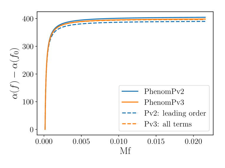
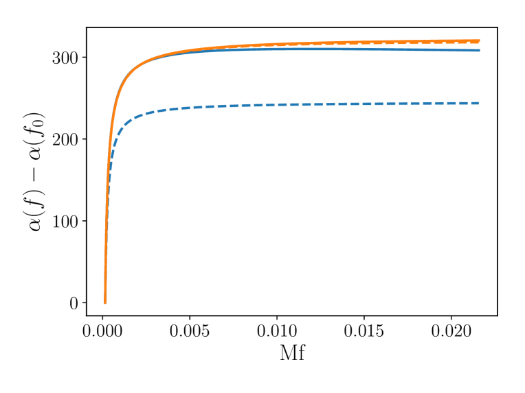
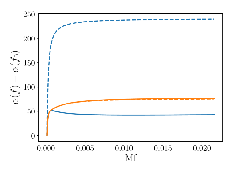
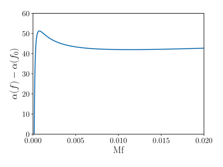
Figure 1: Comparison of leading-order (IMRPhenomPv2: leading order), NNLO (IMRPhenomPv2), full-PN (IMRPhenomPv3: all terms), and the version we adopt in the final model (IMRPhenomPv3) expressions for the precession angle, $\alpha$. First panel: $q=1$, $M_{{\rm{tot}}}=10M_{\odot}$ $\chi_{\rm eff}=0$, $\chi_{p}=0.9$; second panel: $q=8$, $M_{{\rm{tot}}}=10M_{\odot}$ $\chi_{\rm eff}=0$, $\chi_{p}=0.9$; third panel: $q=10$, $M_{{\rm{tot}}}=10M_{\odot}$ $\chi_{\rm eff}=-0.8$, $\chi_{p}=0.1$; fourth panel: same configuration as third panel, but zoom of non-physical behavior of $\alpha_{\rm{v2}}(f)$. All cases are generated from a frequency of $2$ Hz. See text for discussion.

II.5 Upgrading to IMRPhenomPv3

The first closed-form analytic inspiral waveform model for generically precessing BBHs was presented in Chatziioannou et al. (2017a, b). The solution utilized two ingredients. First, the analytic solution to the conservative precession equations constructed in Kesden et al. (2015) was supplemented by radiation-reaction effects through a perturbative expansion in the ratio of the precession to the radiation reaction time scale Klein et al. (2013); Chatziioannou et al. (2013) known as multiple scale analysis (MSA) Bender and Orszag (1999). Second, the frequency-domain waveform was analytically computed through the method of shifted uniform asymptotics (SUA), first introduced in Klein et al. (2014). The resulting inspiral waveform model for the precession dynamics incorporates spin-orbit and spin-spin effects to leading order in the conservative dynamics and up to 3.5PN order in the dissipative dynamics ignoring spin-spin terms.

We use the generic two-spin solution of Chatziioannou et al. (2017a, b) to obtain two-spin expressions for the precession angles $(\alpha_{\rm{v3}},\beta_{\rm{v3}},\epsilon_{\rm{v3}})$. Specifically we use Eqs. (58), (66), (67) and the coefficients in Appendix D in Chatziioannou et al. (2017a) for $\alpha_{\rm{v3}}$ (denoted as $\phi_{z}$ in that paper). Appendix F in Chatziioannou et al. (2017a) provides the analogous equations and coefficients for the $\epsilon_{\rm{v3}}$ angle (called $\zeta$ in Chatziioannou et al. (2017a)), while the $\beta_{\rm{v3}}$ angle (called $\theta_{L}$ in Chatziioannou et al. (2017a)) is given by Equation (8).

As an illustration of the new waveform model we compare IMRPhenomPv2 (blue-dashed) and IMRPhenomPv3 (orange-solid) for a mass-ratio 1:10, two-spin system in Figure 2. The top left panel shows the $h_{\times}(t)$ GW polarisation viewed at an inclination angle of $90\,\rm{deg}$. The top right panel is a zoom in around the merger. At early times both models are in agreement however, due to the difference between the precession angle models the two models start to noticeably disagree around $90\,\rm{s}$ before merger.

Similarly to the angles $\alpha_{\rm{v2}}$ and $\epsilon_{\rm{v2}}$, the expressions for $\alpha_{\rm{v3}}$ and $\epsilon_{\rm{v3}}$ involve series expansions in terms of the GW frequency. The expression for $\epsilon_{\rm{v3}}$ is fully expanded and expressed in terms of a power series of the GW frequency, $f^{-4/3+n/3}$, $n\in[1,6]$. The angle $\alpha_{\rm{v3}}$ involves both expanded ($n\in[1,6]$) and un-expanded terms, a choice made to increase the angle’s accuracy for unequal-mass systems, as discussed in Sec. IV D 1 of Chatziioannou et al. (2017a). The order to which we truncate the relevant expansions can impact the accuracy of the model: too few $n$ terms and the expansion fails to accurately describe the inspiral but too many $n$ terms and the expressions become inaccurate when extrapolating towards higher frequencies. Figure 2 illustrates the impact of expansion order $n$ on the precession angles. The lower-left and lower-middle panels show the $\alpha_{\rm{v3}}$ and $\epsilon_{\rm{v3}}$ angles as a function of the GW frequency. The solid-orange line shows the model that is used in IMRPhenomPv3 and the paler curves show different the result for truncation orders for the $\alpha_{\rm{v3}}$ and $\epsilon_{\rm{v3}}$ models. The dashed-blue line shows the results for the precession angle model used in IMRPhenomPv2 which deviates away from the other approximations. The $\alpha_{\rm{v2}}$ angle in particular shows qualitatively different behaviour, growing rapidly as the frequency increases.

We also have a choice when computing $\beta_{\rm{v3}}$, the angle between $\vec{J}$ and $\vec{L}$. We investigated either using Newtonian order, 2PN Non-Spinning (as was done in IMRPhenomPv2) and also a 3PN version including spin-orbit terms for the magnitude of $\vec{L}$ that is used in the computation of $\beta_{\rm{v3}}$. A comparison between the different methods for calculating $\beta_{\rm{v3}}$ can be seen in the lower-right panel in Fig. 2. The observed modulations are nutation due to spin-spin effects.

The three vertical black lines (from left to right) are the hybrid-MECO Cabero et al. (2017), Schwarzschild ISCO and the ringdown frequency for this system. We assume the limit to which PN results can be reliably used to be near the hybrid-MECO/Schwarzschild ISCO and the region between this and the ringdown frequency to be the region where we are extrapolating the precession angles beyond their assumed region of validity. This assumption appears to hold as it seems to track the location of a turn-over point in many of the precession angle variants, a feature that is unphysical (at least in simple precession cases) as discussed in Sec. II.4.

To decide which choices when computing the precession anlges lead to the most accurate model we performed several mismatch calculation comparing different versions of the model with NR. We find that most choices lead to reasonably accurate models for the inspiral but, however, can lead to suboptimal performance during the merger. We obtain an accurate model for the entire coalescence by using all but the highest order terms in the expressions for $\alpha_{\rm{v3}}$ and $\epsilon_{\rm{v3}}$ and to use the highest order PN calculation available namely, with 3PN with spin-orbit terms when computing $|\vec{L}|$ in the $\beta$ angle. In Sec. III we only show results for the final model.

To minimise differences bewteen IMRPhenomPv2 and IMRPhenomPv3 we adopt the same model for the final spin however, we note a simple extension would be to include all in-plane spin components in the calculation of $S_{\bot}$ and relaxing the approximation that $M_{f}=M_{i}$ by using the final mass model used in the non-precessing case. This will be done in following work.

We also note one other improvement on IMRPhenomPv2, which deals with “superkick” configurations Bruegmann et al. (2008). These are equal-mass configurations where each black hole has the same spin, but the spins both lie in the orbital plane and point in opposite directions. These configurations possess symmetry such that the orbital plane does not precess, but instead “bobs” up and down as linear momentum is radiated perpendicular to the orbital plane. If IMRPhenomPv2 is given the parameters for such a configuration, the definition of $\chi_{p}$, Eq. (3) will yield a non-zero value, and the code will construct the waveform for a precessing system. Neighbouring configurations in parameter space will display similar behaviour, and IMRPhenomPv2 will again generate the “wrong” waveform. By correctly accounting for both spins, IMRPhenomPv3 corrects this problem. A request for an equal-mass superkick configuration will yield the waveform for an equal-mass nonspinning configuration, which is the closest approximation that does not experience recoil.

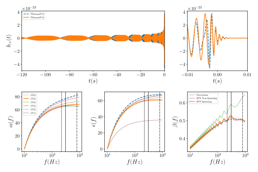
Figure 2: Composite figure comparing the various models for the precession angles and their overall effect on the waveform. We generate the gravitational waveform from a BBH system with the following parameter: $q=10$, $M=20$, $S_{1}=(0.4,0,0.4)$, $S_{2}=(0.3,0,-0.3)$, $f_{{\rm start}}=10$Hz. The top row shows $h_{\times}$ polarisation evaluated at $\iota=\pi/2$ (Here $\iota$ is the angle between $\vec{L}$ and the line of sight). In all panels the dashed blue line corresponds to IMRPhenomPv2 and the solid orange line corresponds to IMRPhenomPv3. Top left: The full waveform generated from 10Hz. Top right: Zoom in around merger. The early-time agreement and late-time disagreement demonstrates the agreement between the two models of precession at low frequencies and disagreement at high frequencies. Bottom row shows the precession angles as a function of GW frequency. Bottom left: $\alpha$. Bottom middle: $\epsilon$. Bottom right: $\beta$. The solid black line is the hybrid-MECO frequency Cabero et al. (2017), the dashed black line is the Schwarzschild ISCO frequency and the dot-dashed black line is the ringdown frequency for this system. The legend in the bottom left plot applies to the bottom middle plot as well and shows to what $n$ order (see text) the $\alpha$ and $\epsilon$ angles where expanded. The legend in the bottom right figure indicates if aligned-spins were included in the calculation of the magnitude of the orbital angular momentum.

III Comparison to numerical relativity

In this section we compare IMRPhenomPv3 to a large number of NR simulations of precessing BBHs and show the excellent agreement between our model and the simulations.

III.1 Mismatch calculation

In GW searches and parameter estimation, template waveforms are correlated with detector data. This operation can be written as an inner-product weighted by the sensitivity of the detector (described by the power spectral density (PSD) $S_{n}(f)$) between the real valued template $h(t)$ and signal $s(t)$ waveforms. We define the overlap between the template and signal as

$$\mathcal{O}\equiv\left(h|s\right)\equiv\,4\,{\rm{Re}}\int\displaylimits_{f_{\rm{min}}}^{f_{\rm{max}}}\frac{\tilde{h}^{*}(f)\tilde{s}(f)}{S_{n}(f)}df\,,$$ (8)

where $\tilde{h}$ representes the Fourier transform of $h$ and $\tilde{h}^{*}$ is the complex conjugate of $\tilde{h}$.

This inner-product is closely related to the definition of the matched-filter signal-to-noise ratio (SNR) and indeed the $1-\mathcal{O}$ between normalised waveforms ($\hat{x}=\sqrt{(x|x)}$) is directly proportional to the loss in SNR making it a useful metric to measure the accuracy of waveform models.

Aside from the masses and spins of the BHs the GW signal depends on a number of extrinsic parameters: the direction of propagation in the source frame ($\iota,\phi_{0}$), a polarisation angle $\psi$, a reference time $t_{0}$ and the luminosity distance $D_{L}$. The dependency of the observed GW signal on the polarisation angle (ignoring the angular position of the source with respect to a detector) is given by

$$h(t)=h_{+}(t)\,{\rm{cos}}(2\psi)+h_{\times}(t)\,{\rm{sin}}(2\psi)\,.$$ (9)

Given two waveforms $h$ and $s$ we quantify the agreement between them by computing their normalised overlap subject to various averages and optimisations of extrinsic parameters whilst keeping the intrinsic parameters fixed. Note that the use of normalised waveforms $\hat{h}$ and $\hat{s}$ factors away the dependency of the $D_{L}$ in the overlap.

In particular for each inclination angle $\iota$ considered we compute the overlap between $\hat{h}$ and $\hat{s}$ with the same masses and spins and vary the extrinsic signal parameters ($\phi^{s}_{0},\psi^{s}_{0}$) by evaluating them on a $10\times 10$ grid with the following domain $\phi^{s}_{0}\in[0,2\pi]$ and $\psi^{s}_{0}\in[0,\pi/4]$. For each point on this grid we analytically maximise over a time shift using an inverse Fourier transform, analytically maximise over $\psi^{h}_{0}$ according to the method detailed in Harry et al. (2016) and finally numerically optimise over $\phi^{h}_{0}$ using optimisation routines from the SciPy package . From here we define the match as a function of the extrinsic parameters of the signal as

$$\mathcal{M}(\phi^{s}_{0},\psi^{s}_{0})\equiv\max_{t^{h}_{0},\phi^{h}_{0},\psi^{h}_{0}}\,(\hat{h}|\hat{s}(\phi^{s}_{0},\psi^{s}_{0}))\,.$$ (10)

Next we average over the extrinsic parameters of the signal $(\phi^{s}_{0},\psi^{s}_{0})$ weighted by its optimal SNR $\rho$ at each point which accounts for the likelihood that this signal would be detected Buonanno et al. (2003); Harry et al. (2018). We call this the orientation-averaged-match

$$\overline{\mathcal{M}}\equiv\left(\frac{\sum\limits_{i}\rho_{i}^{3}\mathcal{M}_{i}^{3}}{\sum\limits_{i}\rho_{i}^{3}}\right)^{1/3}\,.$$ (11)

From here we define the orientation-averaged-mismatch as $1-\overline{\mathcal{M}}$. We will quote results in terms of this. In what follows we shall use $h$ to denote a template waveform, i.e., generated by a waveform approximant and $s$ to denote the signal waveform which will be an NR waveform.

We compute the orientation-averaged-mismatch between the template waveform and each NR waveform at three different inclination angles $(0,\pi/3,\pi/2)\,\rm{rad}$. By increasing the inclination angle we tend to observe a weaker but more modulated waveform due to the precession. We therefore expect the accuracy of the models to decrease at inclined orientations where the effects of precession are typically more prounounced. We consider 3 different waveform approximants: IMRPhenomPv2, our improvement IMRPhenomPv3 and the precessing IMR EOB-NR model SEOBNRv3 Babak et al. (2017). For each NR simulation we generate a template with the same masses and spins beginning from the start frequency as reported in the NR metadata. Waveforms were generated using the LALSimulation package, part of the software library LALSuite lal , using the NR injection infrastructure presented in Schmidt et al. (2017).

When comparing GW signal models with NR there is an ambiguity that one encounters when trying to identify a time (or frequency) in the gravitational waveform and the corresponding retarded time (or frequency) of the BBH dynamics, where spins are measured and defined in the NR simulation Hamilton and Hannam (2018). This complicates the comparison of precessing systems because the orientation of the spin is now time dependent.

To account for the ambiguity in how the spins are defined we allow the frequency at which the spins are specified to vary. This is similar to what was done in Ref. Babak et al. (2017) where SEOBNRv3 was compared to a similar set of NR waveforms. In IMRPhenomPv2 and IMRPhenomPv3 we can fix the start frequency, $f_{\rm{start}}$, and vary the spin-reference-frequency ($f_{\rm{ref}}$), however, in the LALSuite implementation of SEOBNRv3 this is not possible and instead the spins are defined at the start frequency. Therefore we perform the optimisation of spin-reference-frequency slightly differently between the two phenom models and the EOB-NR model. We numerically optimise using SciPy for both cases. For the phenom models we allow $f_{\rm{ref}}$ to vary in the following range $[0.8,1.4]\times f_{\rm{start}}$ and for SEOBNRv3 we vary $f_{\rm{start}}$ in the same range but if $1.4f_{\rm{start}}$ is greater than the maximum start frequency allowed by the EOB-NR generator, $f^{\rm{EOB}}_{\rm{max}}$, then we use this. For long waveforms the variation in the resulting match is less that 1% however, for shorter waveforms, such as SXS:BBH:0165, the variation can be as larger as 8%.

Our NR signal waveforms only contain the $\ell=2$ multipoles which is a good approximation for comparable mass systems $q\lesssim 3$ and for small inclinations where the effect of precession on the waveform is minimised. This assumption breaks down for some of the cases we consider here but we are primarily concerned with how faithful our new model is to a signal which contains the modes that we have modelled. We also want to keep separate systematic errors due to neglecting $\ell>2$ modes and those due to inaccuracies in modelling the $\ell=2$ modes. We compute the match assuming the theoretical design sensitivity of one of the LIGO detectors (zero de-tuned high power PSD ali ) and starting from a low frequency cutoff of $10\,\text{Hz}$ until the end of the waveform. We compute the match over a range of total masses spanning from $20\,M_{\odot}$ to $200\,M_{\odot}$. If the NR waveform is not long enough to start at $10\,\text{Hz}$ then we use the starting frequency of the NR waveform as the low frequency cutoff in the match integral.

III.2 NR catalogue

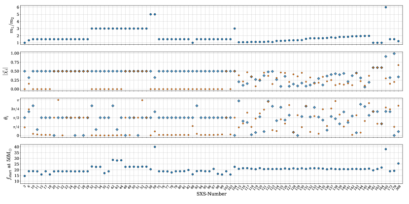
Figure 3: The precessing parameter space we probe using the SXS public catalogue. The x-axis is the SXS catalogue number. The four panels (from top to bottom) show the mass-ratio $q=m_{1}/m_{2}$, the dimensionless spin magnitudes $|\vec{\chi}_{i}|$, the polar angle between the Newtonian orbital angular momentum and the individal BH spin vectors $\theta_{i}$ where $i=1,2$ for the larger and smaller BH respectively and finally the last panel plots the start GW frequency for each simulation when scaled to a total mass of $50\rm{M_{\odot}}$. Where the primary and secondary BHs are plotted as blue diamonds and orange circles respectively.

We use the SXS public catalogue Mroué et al. (2013); sxs of NR waveforms as our validation set consisting of 90 precessing waveforms with mass-ratios between 1:1 and 1:6. Figure 3 presents an illustration of the parameter space covered. This set of NR waveforms mainly covers the mass-ratio space between 1:1 and 1:3 with only 3 waveforms above this: 2 at mass-ratio 1:5 and one at 1:6. This is clearly a heavily undersampled region of parameter space across NR groups (see other public catalogues from RIT Healy et al. (2017); rit and GaTech Jani et al. (2016); gat ). The vast majority of cases also have spin magnitudes that are $\leqslant 0.5$ however there is one case (SXS:BBH:0165) where $|\vec{\chi}|=0.9$. However, this is a short waveform of only 6 orbits in length. Again this highlights the need for longer NR simulations of BBHs with $|\vec{\chi}|>0.5$ across all mass-ratios.

The bottom panel of Fig. 3 illustrates the length of the NR simulations. It shows the start frequency, in Hz, of the $\ell=|m|=2$ GW multipole when the BBH system is scaled to $50M_{\odot}$. In order for a NR waveform to be used in the analysis of LIGO-Virgo data, without hybridising to PN, the waveform needs to span the sensitive region of the detector, a typical start frequency for current instruments is between $20-25\rm{Hz}$ (see Figure 2 of Abbott et al. (2017a)). We see that for a BBH of total mass $50M_{\odot}$, similar to GW150914 Abbott et al. (2016a) (LIGO and Virgo Scientific Collaboration), that many of these cases start at around $20\rm{Hz}$. Again there are a couple of outliers at mass-ratios 1:5 and 1:6.

III.3 Results

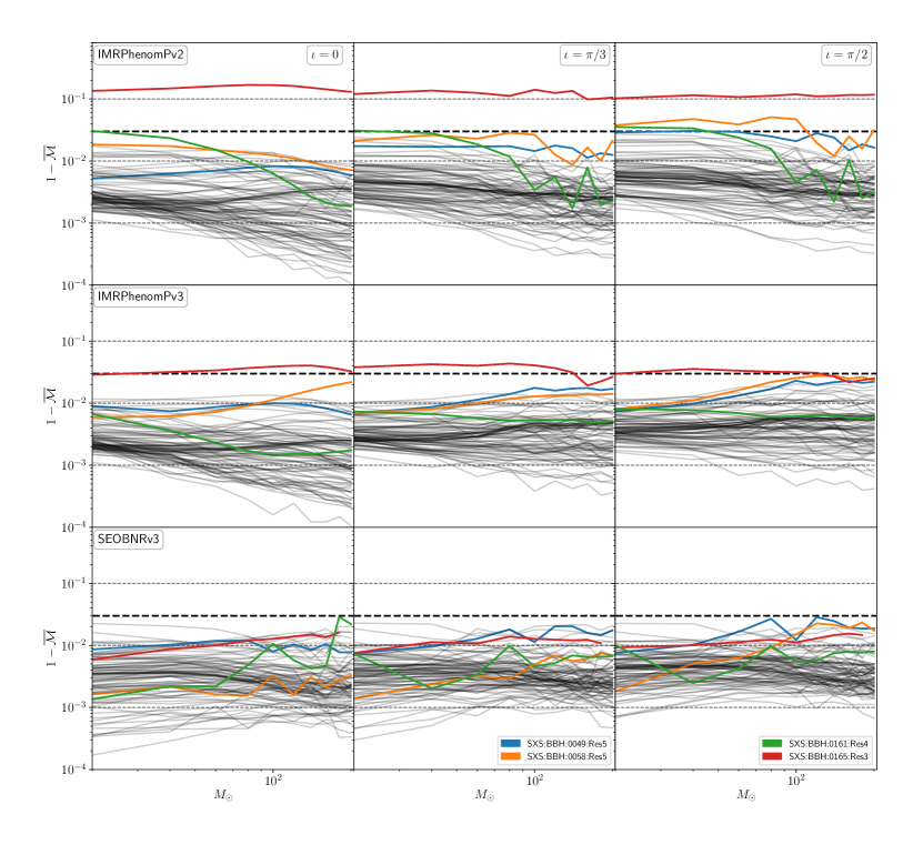
Figure 4: The results of the comparison between IMRPhenomPv2 (first row), IMRPhenomPv3 (second row) and SEOBNRv3 (third row) and the precessing NR simulations from the public SXS catalogue. Each column shows the results for $\iota=(0,\pi/3,\pi/2)$, from left to right. Where $\iota$ is the angle between the Newtonian orbital angular momentum $\vec{L}$ and the line-of-sight, at the start frequency. The figure shows the orientation-averaged-mismatch ($1-\overline{\mathcal{M}}$) as a function of the total mass (log scale). Cases which have a maximum mismatch greater than $3\%$ are coloured and presented in Table 1.

Figure 4 shows the results of the orientation-averaged-mismatch ($1-\overline{\mathcal{M}}$) calculation as a function of the total mass. Each row corresponds to a fixed template waveform labeled in the top left of each plot in the first column. From top to bottom each row show results for IMRPhenomPv2, IMRPhenomPv3 and SEOBNRv3. From left to right each column corresponds to the three different inclination angles we tested $0,\pi/3$ and $\pi/2$ respectively.

First we note that, for all three models, the majority of cases have mismatches smaller that $3\%$ and many smaller than $1\%$. This is in agreement with the findings of Ref Babak et al. (2017). Interestingly we find that the mismatch varies weakly with inclination angle indicating that the models perform well even when precession effects are amplified. One of the key results is the superior performance of IMRPhenomPv3 for total masses between $20-50M_{\odot}$ where all but one case (SXS:BBH:0165 is discussed below) have mismatches $\lesssim 1\%$. We attribute this to the more accurate and reliable new model of the precession dynamics of Chatziioannou et al. (2017a, b).

To highlight regions of parameter space where current models are least accurate we have compiled Table 1, which lists the SXS catalogue number, their mass-ratio and initial spin components if at any point the mismatch is greater than $3\%$. In the table we report the orientation-averaged-mismatch averaged over all total masses for each inclination angle. We also colour these cases in Figure 4.

Our expectation that higher mass-ratio systems will yield the least accurate results due to the fact that precession is based on a PN model and not calibrated to NR, is borne out in our results. Out of all the worst cases, with the exception of SXS:BBH:0161, the worst cases have mass-ratios $\geqslant 3$. SXS:BBH:0161 is the only equal-mass outlier with worst mismatch marginally greater than $3\,\%$ for IMRPhenomPv2. For IMRPhenomPv3 and SEOBNRv3 the accuracy is better than $1\,\%$ for all the vast majority of cases.

Waveform Model	IMRPhenomPv2			IMRPhenomPv3			SEOBNRv3
SXS:BBH:ID	$0$	$\pi/3$	$\pi/2$	$0$	$\pi/3$	$\pi/2$	$0$	$\pi/3$	$\pi/2$
0049 [$q=3$, $\vec{S}_{1}=(0.5,0,0)$, $\vec{S}_{2}=(0,0,0.5)$]	0.7	1.5	2.4	0.9	1.4	1.8	1.0	1.5	1.8
0058 [$q=5$, $\vec{S}_{1}=(0.5,0,0)$, $\vec{S}_{2}=(0,0,0)$]	1.2	2.0	3.3	1.3	1.2	2.2	0.2	0.5	1.4
0161 [$q=1$, $\vec{S}_{1}=(0.52,0,-0.3)$, $\vec{S}_{2}=(0.52,0,-0.3)$]	1.0	1.1	1.4	0.2	0.6	0.7	0.8	0.6	0.7
0165 [$q=6$, $\vec{S}_{1}=(0.74,0.19,-0.50)$, $\vec{S}_{2}=(-0.19,0,-0.23)$]	15.4	12.5	12.1	3.6	3.5	3.0	1.2	1.1	1.3

Table 1: Percentage mismatches averaged over all total masses for each the three inclination angles (rad) considered. All cases that have a mismatch larger than $3\%$ are shown. The first column shows the SXS ID number with the mass-ratio and initial spin vectors in parentheses.

The case with the highest mismatch, across all templates, is SXS:BBH:0165. This is a mass-ratio 1:6 system with initial spins $S_{1}=(0.74,0.19,-0.50)$ and $S_{2}=(-0.19,0,-0.23)$ with a length of $\sim 6.5$ orbits. IMRPhenomPv2 has a best mismatch of $\sim 12\%$. IMRPhenomPv3 substantionally improves upon this with a worst mismatch of $\sim 3.6\%$. SEOBNRv3 performs well achieving a worst mismatch of $\sim 1.3\%$. Given that the precession, in all three IMR models, is modelled with uncalibrated PN or EOB calculations, it is not surprising that the region of parameter space where the models do worst comes from high mass-ratios and high spin magnitudes. This is, by far, the case with the most dramatic improvement. In terms of its place in parameter space it has the largest mass-ratio and spin magnitude.

Out of the two mass-ratio 1:5 systems one of them has a worst mismatch larger than $3\%$. This case, SXS:BBH:0058, is also the longest mass-ratio 1:5 case with approximately 28 orbits. We improve from a worst mismatch of $3.3\%$ with IMRPhenomPv2 to $2.2\%$ with IMRPhenomPv3. SEOBNRv3 shows good agreement with a worst average mismatch of $\sim 1.4\,\%$.

For cases with mass-ratio 1:3 we find that only 1 (SXS:BBH:0049) out of the 15 cases has a mismatch larger than $3\%$. The mismatch is worst for IMRPhenomPv2 and only goes marginally above $3\,\%$ for the $\iota=\pi/2$ case where we expect the effects of precession to be most pronouced. With IMRPhenomPv3 we improve, across all inclinations, with average mismatches between $1-2\,\%$. We find a similar performance with SEOBNRv3.

Note however, that all the mass-ratio 1:3 and 1:5 systems all have spin magnitudes $\leqslant 0.5$. Validating precessing waveform models at large spin magnitudes requires more NR simulations to be performed. We highlight again that these comparisons only include the $\ell=2$ multipoles in the signal waveform and for larger mass-ratio systems $(q\gtrsim 3)$ negleting the higher multipoles is no longer a good approximation to the full GW signal.

IV GW151226 analysis

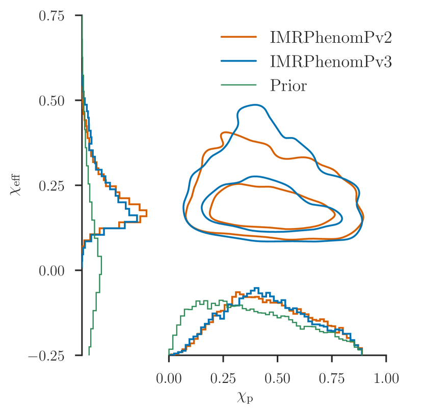
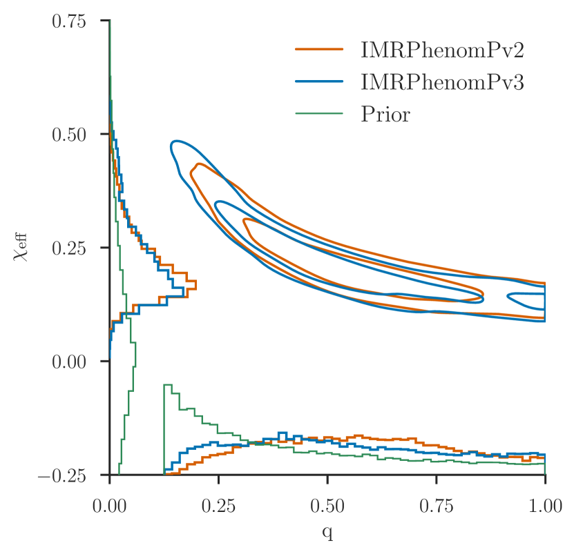
Figure 5: Posterior probability densities for $\chi_{\text{eff}}-\chi_{p}$ (left) and $\chi_{\text{eff}}-q$ (right) for GW151226 using IMRPhenomPv2 and IMRPhenomPv3. Despite the more accurate description of 2-spin dynamics of IMRPhenomPv3 the posteriors are consistent, demonstrating the difficulty of measuring 2-spin dynamics.

As a first application of the new IMRPhenomPv3 model we study whether the improved two-spin prescription allows for improved parameter extraction from existing GW signals. We focus on event GW151226 as it is the only system with strong support for at least one spinning BH Abbott et al. (2016b) (LIGO and Virgo Scientific Collaboration); Vitale et al. (2017). In spite of this, GW151226 has never been analyzed with a precessing model that employs two-spin dynamics: on the one hand, GW151226 has a low-enough total mass that an analysis with SEOBNRv3 is not computationally feasible; simultaneously, GW151226 is so massive that the merger phase of the coalescence is in band, making an analysis with precessing inspiral-only models, such as SpinTaylorT4, incomplete.

The new IMRPhenomPv3 waveform model constructed here meets both criteria of computational efficiency and full coalescence description, allowing us to perform the first two-spin analysis of GW151226. We use the Bayesian Inference code LALInferenceNest Veitch et al. (2015) and publicly available data from the LIGO Open Science Centre (LOSC, losc.ligo.org). We estimate the power spectral density noise using on-source data and the BayesWave algorithm Littenberg and Cornish (2015); Cornish and Littenberg (2015). We marginalise over detector calibration amplitude and phase uncertainty using values provided in Abbott et al. (2016f). We use a spin prior that is uniform in direction and magnitude up to $0.89$. In what follows, we present and compare results obtained using IMRPhenomPv2 using a reduced-order-quadrature approximation to the likelihood Smith et al. (2016) and IMRPhenomPv3.

Table 2 presents our results for the intrinsic parameters. We quote the median value from the 1-D marginalised posterior and the associated $90\%$ symmetric credible interval. Noteworthy differences are a broader uncertainty in the primary mass resulting in IMRPhenomPv3 favouring a slightly more asymmetric system, although both models are within the statistical uncertainty of each other. Overall we find consistent results between the two models as well as the published LIGO-Virgo Collaboration (LVC) analysis Abbott et al. (2016f). We also have an estimate of the Bayes factor for a coherent signal across the two LIGO detectors versus an incoherent signal or noise. We find a slightly larger Bayes factor for IMRPhenomPv3 despite the extra degrees of freedom from the full 2-spin description

Figure 5 shows the 2-dimensional posterior densities for $\chi_{\text{eff}}-\chi_{p}$ (left) and $\chi_{\text{eff}}-q$ (right) obtained from both waveform models as well as the 1-dimensional prior distributions. Both plots demonstrate broad agreement with IMRPhenomPv3 marginally favoring more unequal masses. This result is also consistent based on the comparisons to NR waveforms presented in the previous section. The posterior for $\chi_{p}$ is consistent with its prior, confirming the absence of evidence of spin-precession in GW151226. Overall we find that a re-analysis of the merger event GW151226 with our new waveform model does not provide new insights into the nature of the source but instead reinforces our current understanding of the source.

The consistency of the results implies that two-spin precession effects do not impact this signal in agreement with previous studies predicting that aligned-two-spin effects are not easily measurable Pürrer et al. (2016). However, it is possible that certain binaries and orientations might make it possible to measure both spins simultaneously. This could be achieved, for example, with precessing models that also include higher multipoles modes, or with louder signals observed by more detectors.

Parameter	IMRPhenomPv2	IMRPhenomPv3
Primary Mass: $m_{1}(M_{\odot})$	$13.68^{+7.93}_{-3.13}$	$14.45^{+10.23}_{-3.96}$
Secondar Mass: $m_{2}(M_{\odot})$	$7.73^{+2.10}_{-2.41}$	$7.35^{+2.57}_{-2.52}$
Total Mass: $M_{\rm{tot}}(M_{\odot})$	$23.37^{+6.00}_{-1.10}$	$23.80^{+8.33}_{-1.55}$
Mass ratio: $q$	$0.57^{+0.36}_{-0.32}$	$0.51^{+0.44}_{-0.31}$
Effective Spin: $\chi_{\rm{eff}}$	$0.19^{+0.18}_{-0.07}$	$0.20^{+0.23}_{-0.09}$
Precession Parameter: $\chi_{\rm{p}}$	$0.44^{+0.34}_{-0.28}$	$0.44^{+0.35}_{-0.28}$
Log Bayes Factor: $\rm{Log}(\mathcal{B})$	50.707	51.291

Table 2: Parameter Table for GW151226. Masses are defined in the source frame. We quote the median and the 90% symmetric credible interval of the 1D marginalised posterior distributions.

V Discussion

We have presented an upgrade to the phenomenological model IMRPhenomPv2 called IMRPhenomPv3. This model predicts the GW polarisations computed using the the dominant $\ell=|m|=2$ multipole in the co-precessing frame, from non-eccentric merging BBHs with generically orientated spins. Our upgrade consists of replacing the model for the precession dynamics of Hannam et al. (2014) that was derived under the assumption of a single spin precessing BBH system with the more accurate analytic model from Chatziioannou et al. (2017a, b) that contains two-spin effects.

We have validated our new model against a large set of precessing NR waveforms. Although our selection of NR waveforms is biased towards mass-ratios $<3$ and spin magnitudes $<0.5$ we find that all three models considered generally perform well however, we have identified a clear region in parameter space, mass-ratios $>3$ where all models begin to loose accuracy. Encouragingly we find that IMRPhenomPv3 greatly outperforms the previous model for the most extreme case we considered, with the largest improvement being $\sim 12\%$. This improvement suggests that IMRPhenomPv3 can be utilised in a much wider parameter space than IMRPhenomPv2 was found to be reliable. We emphasise the importance of NR to continue to push the capabilities of precessing BBH simulations that will allow more stringent tests of waveforms models and ultimately lead to more accurate waveform models being developed.

As a first application we re-analysed GW151226 with our two-spin model and find consistent results compared with the single-spin model thereby reinforcing our current inference on the nature of GW151226.

As our waveform model is analytic one can evaluate the model using a non-uniform grid of frequencies. This is essential for methods such as ROQ Smith et al. (2016) and the multi-banding technique of Vinciguerra et al. (2017). These methods can increase the computational efficiency of sampling-based parameter estimation by factors of 300 for low mass systems.

Finally we note that there are a number of physical effects that are ignored. We do not model any asymmetry between the positive and negative $m$ modes which are responsible for large out-of-plane recoil kick velocities. In the underlying, aligned-spin model we do not include effects from higher order multipoles however, we have recently developed a method to do this London et al. (2018) and we are currently determining the accuracy of a precessing model that includes higher order multipoles in the co-precessing frame.