Trading Strategies Generated Pathwise
by Functions of Market Weights

Abstract

Almost twenty years ago, E.R. Fernholz introduced portfolio generating functions which can be used to construct a variety of portfolios, solely in the terms of the individual companies’ market weights. I. Karatzas and J. Ruf developed recently another methodology for the functional construction of portfolios, which leads to very simple conditions for strong relative arbitrage with respect to the market. In this paper, both of these notions of functional portfolio generation are generalized in a pathwise, probability-free setting; portfolio generating functions, possibly less smooth than twice-differentiable, involve the current market weights, as well as additional bounded-variation functions related to the market weights. This generalization leads to a wider class of functionally-generated portfolios than was heretofore possible, to novel methods for dealing with the “size” and “momentum” effects, and to improved conditions for outperforming the market portfolio over suitable time-horizons.

Keywords and Phrases: Stochastic portfolio theory, pathwise Itô formula, pathwise Tanaka formula, trading strategies, functional generation, regular functions, strong relative arbitrage, size effect, momentum effect.

1 Introduction

The concept of ‘functionally generated portfolios’ was introduced by Fernholz, (1999, 2002) and has been one of the essential components of stochastic portfolio theory; see Fernholz and Karatzas, (2009) for an overview. Portfolios generated by appropriate functions of the individual companies’ market weights have wealth dynamics which can be expressed solely in terms of these weights, and do not involve any stochastic integration. Constructing such portfolios does not require any statistical estimation of parameters, or any optimization. Completely observable quantities such as the current values of ‘market weights’, whose temporal evolution is modeled in terms of continuous semimartingales, are the only ingredients needed for building these portfolios. Once this structure has been discerned, the mathematics underpinning its construction involves just a simple application of Itô’s rule. Then the goal is to construct such portfolios that outperform a reference portfolio, for example, the market portfolio, under appropriate structural conditions.

Karatzas and Ruf, (2017) recently found a new way for the functional generation of trading strategies, which they call ‘additive generation’, as opposed to Fernholz’s ‘multiplicative generation’, of portfolios. This new methodology weakens the assumptions on the market model: asset prices and market weights are continuous semimartingales, and trading strategies are constructed from ‘regular’ functions of the semimartingales without the help of stochastic calculus. Trading strategies generated in this additive manner require simpler conditions for strong relative arbitrage with respect to the market over appropriate time horizons; see also Fernholz et al., (2018).

Along a different, but related, development, Föllmer, (1981) showed almost 40 years ago that certain aspects of Itô calculus can be developed ‘path by path’, without any probability structure. Once a given function admits the pathwise property of quadratic variation/covariation along a given nested sequence of partitions over a fixed time interval of finite length, this new type of Itô’s change of variable formula can be proven by an application of Taylor expansion in a surprisingly simple way. Then Wuermli, (1980) introduced in this same setting the concept of local times and the corresponding pathwise Tanaka formula, in a pathwise sense. This allows the change of variable formula to be applied to less regular functions, by involving appropriately defined pathwise local times. These concepts of local times have been further developed recently; see Perkowski and Prömel, (2015), Davis et al., (2018), and Cont and Perkowski, (2018).

In this paper, we generalize both additive and multiplicative functional generation of trading strategies in several ways. First, we use pathwise Itô calculus to show that one can construct trading strategies, generated additively or multiplicatively from a given function, depending on the market weights and in a manner completely devoid of probability considerations. The only analytic structure we impose is that the market weights admit continuous covariations in a pathwise sense. Secondly, we admit generating functions that depend on an additional argument of finite variation. Introducing new arguments, other than the market weights, gives extra flexibility in constructing portfolios; see Strong, (2014), Schied et al., (2018), Ruf and Xie, (2018). We present various types of additional such arguments, to the effect that a variety of new trading strategies can be generated from a function depending on them; these strategies yield new sufficient conditions for strong relative arbitrage with respect to the market portfolio. Then, we show how to apply the pathwise Tanaka formula to construct portfolios from generating functions rougher than heretofore possible. In order to use the Itô formula, a function needs to be at least twice-differentiable, whereas the Tanaka formula requires less smooth functions, namely, absolutely continuous. Thus, usage of the Tanaka formula broadens the class of portfolio-generating functions very considerably.

We also present new sufficient conditions for strong relative arbitrage via additively and multiplicatively generated trading strategies. The existing sufficient condition in Karatzas and Ruf, (2017) requires the generating function to be ‘Lyapunov’, or the corresponding ‘Gamma function’ to be nondecreasing. By contrast, the new sufficient conditions in this paper depend on the intrinsic nondecreasing structure of the generating function itself. This new condition shows that trading strategies outperforming the market portfolio can be generated from a much richer collection of functions depending on the market weights and on an additional argument of finite variation. We provide some interesting examples of such trading strategies, and empirical analysis of them.

Preview : Section 2 presents the elements of the pathwise Itô calculus that will be needed for our purposes. Section 3 defines trading strategies and regular functions, then discusses how to generate trading strategies from regular functions in ways both additive and multiplicative. Section 4 gives sufficient conditions for such trading strategies to generate strong relative arbitrage with respect to the market. Section 5 shows methods of generating trading strategies in a similar manner as in Section 3, but from less smoother functions with help of relevant notion of local time and Tanaka formula. Section 6 gives some examples of trading strategies generated from entropic functions and corresponding sufficient conditions for strong arbitrage. Section 7 contains empirical results of portfolios discussed in Section 6. Finally, Section 8 concludes.

2 Pathwise Itô calculus

In what follows, we let $X=(X_{1},\cdots,X_{d})^{\prime}$ be a $[0,\infty)^{d}$-valued continuous function, representing a $d$-dimensional vector of assets whose values change over time. Each component is defined on $[0,T]$, for a fixed $T>0$, and $X_{i}(t)$ stands for the value of the $i$^th asset at time $t\in[0,T]$.

We require the components of $X$ to admit continuous covariations in the pathwise sense with respect to a given, refining sequence $(\mathbb{T}_{n})_{n\in\mathbb{N}}$ of partitions of $[0,T]$. The sequence $(\mathbb{T}_{n})_{n\in\mathbb{N}}$ is such that each partition is of the form $\mathbb{T}_{n}=\{0=t_{0}^{(n)}<t_{1}^{(n)}<\cdots<t^{n}_{N(\mathbb{T}_{n})}=T\}$ for $n\in\mathbb{N}$, as well as $\mathbb{T}_{1}\subset\mathbb{T}_{2}\subset\cdots$, and the mesh size $||\mathbb{T}_{n}||:=\max_{[t_{j},t_{j+1}]\in\mathbb{T}_{n}}|t_{j+1}-t_{j}|$ decreases to zero as $n\rightarrow\infty$. We fix such a sequence $(\mathbb{T}_{n})_{n\in\mathbb{N}}$ of partitions for the remainder of the paper.

Here and below, the notation $[t_{j},t_{j+1}]\in\mathbb{T}_{n}$ means that $t_{j}$ and $t_{j+1}$ are consecutive points in the partition $\mathbb{T}_{n}$, i.e., $t_{j}<t_{j+1}$, $\mathbb{T}_{n}\cap(t_{j},t_{j+1})=\emptyset$. Also, when we write $[t_{j},t_{j+1}]\in\mathbb{T}_{n}$ and $t_{j}\leq t$ simultaneously, we set $t_{j+1}=t$ when $j$ is the biggest index satisfying $t_{j}\leq t$. With this notation, we present the notion of the pathwise quadratic covariation of $X$ along $(\mathbb{T}_{n})_{n\in\mathbb{N}}$, as follows.

Definition 2.1.

A continuous function $X=(X_{1},X_{2},\cdots,X_{d})^{\prime}$ is said to have a pathwise quadratic covariation along a given nested sequence of partitions $(\mathbb{T}_{n})_{n\in\mathbb{N}}$ of $[0,T]$, if the limit of the sequence

$$\sum_{\begin{subarray}{c}[t_{j},t_{j+1}]\in\mathbb{T}_{n}\\ t_{j}\leq t\end{subarray}}\big{(}X_{i}(t_{j+1})-X_{i}(t_{j})\big{)}\big{(}X_{k}(t_{j+1})-X_{k}(t_{j})\big{)},\qquad n\in\mathbb{N}$$ (2.1)

exists for any $t\in[0,T]$ as $n\rightarrow\infty$ and the resulting mapping, denoted by $t\mapsto\langle X_{i},X_{k}\rangle(t)$, is real-valued and continuous for every $1\leq i,k\leq d$. We call $\langle X_{i},X_{k}\rangle$ the pathwise quadratic covariation of $X_{i}$ and $X_{k}$, and define the pathwise quadratic variation of $X_{i}$ by $\langle X_{i}\rangle:=\langle X_{i},X_{i}\rangle$ as usual.

We stress that the existence of pathwise covariations and quadratic variations for the components of $X$ depends heavily on the choice of the nested, or “refining” sequence $(\mathbb{T}_{n})_{n\in\mathbb{N}}$ of partitions. Example 5.3.2 in Cont, (2016), and the arguments following, illustrate this fact. We note also that the existence of pathwise covariations and quadratic variations is required for Itô’s formula to hold in a pathwise sense.

Next, we state the original one-dimensional pathwise Itô formula, introduced by Föllmer, (1981).

Theorem 2.2 (Pathwise Itô formula for paths with quadratic variation, Föllmer, (1981)).

Fix a continuous function $X$ which admits the quadratic variation along the given nested sequence of partitions $\mathbb{T}=(\mathbb{T}_{n})_{n\geq 1}$ of $[0,T]$. Then for every $C^{2}(\mathbb{R},\mathbb{R})$ function $f$, the pathwise change of variable formula

$$f\big{(}X(t)\big{)}-f\big{(}X(0)\big{)}=\int_{0}^{t}f^{\prime}\big{(}X(s)\big{)}dX(s)+\frac{1}{2}\int_{0}^{t}f^{\prime\prime}\big{(}X(s)\big{)}d\langle X\rangle(s)$$ (2.2)

holds for $t\in[0,T]$. Here, the Föllmer-Itô integral is defined as the pointwise limit

$$\int_{0}^{t}f^{\prime}\big{(}X(s)\big{)}dX(s):=\lim_{n\rightarrow\infty}\sum_{\begin{subarray}{c}[t_{j},t_{j+1}]\in\mathbb{T}_{n}\\ t_{j}\leq t\end{subarray}}f^{\prime}(X(t_{j}))(X(t_{j+1})-X(t_{j})),$$ (2.3)

and the last integral of the right-hand side of (2.2) is Lebesgue-Stieltjes integral.

We will need also the pathwise Itô formula in a higher-dimensional setting than Theorem 2.2, and with an extra ‘input’ as additional argument. For this purpose, we let $A=(A_{1},A_{2},\cdots,A_{m})^{\prime}$ be an additional vector function of finite variation and consider a $(d+m)$-dimensional function $f\big{(}X_{1}(t),\cdots,X_{d}(t),\allowbreak A_{1}(t),\cdots,A_{m}(t)\big{)}$ of time $t\in[0,T]$. We say that a given function $f:\mathbb{R}^{d+m}\rightarrow\mathbb{R}$ is in $\mathbb{C}^{j,k}(\mathbb{R}^{(d+m)},\mathbb{R})$, if it is $j$-times continuously differentiable with respect to the first $d$ components and $k$-times continuously differentiable to the last $m$ components. We also denote by $\partial_{i}f$ the $i$^th partial derivative, and by $D_{\ell}f$ the $(d+\ell)$^th partial derivative of $f$.

We now present the following version of the pathwise Itô formula involving both $X$ and $A$. The proof is given in the Appendix, and the idea of proof is the same as that of Föllmer’s original Theorem.

Theorem 2.3 (Multidimensional pathwise Itô formula).

Fix a $d$-dimensional continuous function $X$ having pathwise quadratic covariations along a given sequence of partitions $\mathbb{T}=(\mathbb{T}_{n})_{n\geq 1}$ of $[0,T]$, and an $m$-dimensional continuous function $A$ of finite variation defined on $[0,T]$. Then for every $f\in\mathbb{C}^{2,1}(\mathbb{R}^{(d+m)},\mathbb{R})$, the pathwise change of variable formula

$$f\big{(}X(t),A(t)\big{)}-f\big{(}X(0),A(0)\big{)} =\int_{0}^{t}\nabla f\big{(}X(s),A(s)\big{)}dX(s)+\sum_{\ell=1}^{m}\int_{0}^{t}D_{\ell}f\big{(}X(s),A(s)\big{)}dA_{\ell}(s)$$

$$+\frac{1}{2}\sum_{i,k=1}^{d}\int_{0}^{t}\partial^{2}_{i,k}f\big{(}X(s),A(s)\big{)}d\langle X_{i},X_{k}\rangle(s)$$ (2.4)

holds for $t\in[0,T]$. Here the Föllmer-Itô integral is defined as the pointwise limit

$$\int_{0}^{t}\nabla f\big{(}X(s),A(s)\big{)}dX(s):=\lim_{n\rightarrow\infty}\sum_{\begin{subarray}{c}[t_{j},t_{j+1}]\in\mathbb{T}_{n}\\ t_{j}\leq t\end{subarray}}\sum_{i=1}^{d}\partial_{i}f\big{(}X(t_{j}),A(t_{j})\big{)}\big{(}X_{i}(t_{j+1})-X_{i}(t_{j})\big{)},$$ (2.5)

whereas the other integrals of the right-hand side of (2.4) are Lebesgue-Stieltjes integrals.

3 Trading strategies generated in pathwise sense

As in the previous section, we consider a $[0,\infty)^{d}$-valued, continuous function $X=(X_{1},\cdots,X_{d})^{\prime}$ which admits continuous covariations with respect to a refining sequence $(\mathbb{T}_{n})_{n\in\mathbb{N}}$ of partitions of $[0,T]$; we also let $A=(A_{1},\cdots,A_{m})^{\prime}$ be an additional vector function of finite variation. For the purposes of this section, the components of $X$ will denote the value processes of $d$ tradable assets, and eventually stand for the market weights in an equity market. At the same time, the components of $A$ will model the evolution of an observable, but non-tradable, quantity related to these market weights.

For a subset $V$ of a Euclidean space, we denote by $C([0,T],V)$ the space of continuous $V$-valued functions defined on $[0,T]$; whereas $CBV([0,T],V)$ stands for the space of those functions in $C([0,T],V)$ which are of bounded variation. With this notation, we have the following definition of trading strategy with respect to the pair $(X,A)$, in the manner of Karatzas and Ruf, (2017).

Definition 3.1 (Trading strategies).

For the pair $(X,A)$ of a $d$-dimensional function $X\in C([0,T],\mathbb{R}^{d})$ and an $m$-dimensional function $A\in CBV([0,T],\mathbb{R}^{m})$, suppose that $\vartheta=(\vartheta_{1},\cdots,\vartheta_{d})^{\prime}$ is a $d$-dimensional function with representation

$$\vartheta_{i}(\cdot)=\Theta_{i}\big{(}X(\cdot),A(\cdot)\big{)},\qquad i=1,\cdots,d.$$ (3.1)

Here, $\Theta=(\Theta_{1},\cdots,\Theta_{d})^{\prime}$ is a vector of functions, for which we can define an integral $\int_{0}^{\cdot}\vartheta(t)dX(t)\equiv\int_{0}^{\cdot}\sum_{i=1}^{d}\vartheta_{i}(t)dX_{i}(t)$ with respect to $X$; we write $\vartheta\in\mathscr{L}(X,A)$, to express this. We shall say that $\vartheta\in\mathscr{L}(X,A)$ is a trading strategy with respect to $X$, if it is ‘self-financed’ in the sense that

$$V^{\vartheta}(\cdot;X)-V^{\vartheta}(0;X)=\int^{\cdot}_{0}\sum^{d}_{i=1}\vartheta_{i}(t)dX_{i}(t)$$ (3.2)

holds. In (3.2) and in what follows,

$$V^{\vartheta}(t;X):=\sum^{d}_{i=1}\vartheta_{i}(t)X_{i}(t),\qquad 0\leq t\leq T$$ (3.3)

denotes the value process of the strategy $\vartheta$ at time $t$.

The interpretation is that $\vartheta_{i}(t)$ stands for the “number of shares” invested in asset $i$ at time $t$. If $X_{i}(t)$ is the price of this asset, then $\vartheta_{i}(t)X_{i}(t)$ is the dollar amount invested in asset $i$ at time $t$, and $V^{\vartheta}(t;X)$ the total value of investment across all assets. “Self-financing” means that there are neither infusions nor withdrawals of capital: gains are re-invested, losses have to be absorbed. We shall write $V^{\vartheta}(\cdot)$ instead of $V^{\vartheta}(\cdot;X)$ whenever the integrator $X$ is fixed and apparent from the context.

The preceding pathwise Itô formula in Theorem 2.3 suggests that integrands $\vartheta\in\mathscr{L}(X,A)$ of the special form $\vartheta(t)=\nabla f\big{(}X(t),A(t)\big{)}$, for some function $f\in\mathbb{C}^{2,1}(\mathbb{R}^{(d+m)},\mathbb{R})$, play a very important role for integrators $X\in C([0,T],\mathbb{R}^{d})$ that admit finite quadratic covariations $\langle X_{i},X_{j}\rangle$, $1\leq i,j\leq d$ along an appropriate nested sequence of partitions. This gives rise to the following definition.

Definition 3.2 (Admissible trading strategy).

Let $X$ be a $d$-dimensional function in $C([0,T],\mathbb{R}^{d})$, and $A$ an $m$-dimensional function in $CBV([0,T],\mathbb{R}^{m})$. A $d$-dimensional trading strategy $\vartheta:[0,\infty)\rightarrow\mathbb{R}^{d}$ in $\mathscr{L}(X,A)$ is called admissible trading strategy for the pair $(X,A)$, if there exists a function $G:\mathbb{R}^{d}\times\mathbb{R}^{m}\rightarrow\mathbb{R}$ in the space $\mathbb{C}^{2,1}(\mathbb{R}^{(d+m)},\mathbb{R})$, such that (3.1) holds for $\Theta_{i}=\nabla_{i}G$; that is,

$$\vartheta(t)=\nabla G\big{(}X(t),A(t)\big{)},\qquad 0\leq t\leq T.$$ (3.4)

If $\vartheta$ is an admissible trading strategy for $(X,A)$, the last integral of (3.2) above is interpreted as a pathwise Föllmer-Itô integral in the context of Theorem 2.3. In an what follows, we will define a regular function for the pair $(X,A)$, consisting of a $d$-dimensional continuous function $X$, and an $m$-dimensional function $A$ in $CBV([0,T],\mathbb{R}^{m})$.

Definition 3.3 (Regular function).

We say that a function $G:\mathbb{R}^{d}\times\mathbb{R}^{m}\rightarrow\mathbb{R}$ in $\mathbb{C}^{2,1}(\mathbb{R}^{(d+m)},\mathbb{R})$ is regular for the pair $(X,A)$, consisting of a $d$-dimensional continuous function $X$ and of a function $A\in CBV([0,T],\mathbb{R}^{m})$, if the continuous function

$$\Gamma^{G}(t):=G\big{(}X(0),A(0)\big{)}-G\big{(}X(t),A(t)\big{)}+\int^{t}_{0}\nabla G\big{(}X(s),A(s)\big{)}dX(s),\quad 0\leq t\leq T$$ (3.5)

has finite variation on compact intervals of $[0,T]$.

Remark 3.4.

In order to define a pathwise Föllmer-Itô integral and be able to use the pathwise Itô calculus, we need a sufficiently smooth (in general, at least $\mathbb{C}^{2,1}$) function $G$, and an integrand which can be cast in the form of a derivative $\nabla G$ of this function in the manner of (3.4). Thus, thanks to the above definition, we can always apply the pathwise Itô formula (Theorem 2.3) to the function $G$ as in Definition 3.3 above, and obtain another expression for the so-called “Gamma function” $\Gamma^{G}(\cdot)$ in (3.5); namely,

$$\Gamma^{G}(t)=-\sum_{\ell=1}^{m}\int_{0}^{t}D_{\ell}G\big{(}X(s),A(s)\big{)}dA_{\ell}(s)-\frac{1}{2}\sum_{i,k=1}^{d}\int_{0}^{t}\partial_{i,k}^{2}G\big{(}X(s),A(s)\big{)}d\langle X_{i},X_{k}\rangle(s).$$ (3.6)

Here we recall that $D_{\ell}G\big{(}X(s),A(s)\big{)}$ and $\partial_{i,k}^{2}G\big{(}X(s),A(s)\big{)}$ are, respectively, the first-order $(d+\ell)$^th partial derivative and the second-order $(i,k)$^th partial derivative of $G$ at $\big{(}X(s),A(s)\big{)}$.

The difference in Definition 3.3 here, with Definition 3.1 of Karatzas and Ruf, (2017), should be noted and stressed. In Karatzas and Ruf, (2017), the integrand $\vartheta_{i}$ need not be the form of ‘gradient’ of a regular function $G$. Here, the special structure of (3.4) for the integrand is necessary; this is the “price one has to pay” for being able to work in a pathwise, probability-free setting, without having to invoke the theory of rough paths.

3.1 Trading strategies depending on the market weights

We place ourselves from now onward in a frictionless equity market with a fixed number $d\geq 2$ of companies. We also consider a vector of continuous functions $S=(S_{1},\cdots,S_{d})^{\prime}\in C([0,T],[0,\infty)^{d})$, where $S_{i}(t)$ represents the capitalization of the $i^{\text{th}}$ company at time $t\in[0,T]$. Here we take $S_{i}(0)>0$ and allow $S_{i}(t)$ to vanish at some time $t>0$, for all $i=1,\cdots,d$; but we assume also that the total capitalization $\Sigma(t):=S_{1}(t)+\cdots+S_{d}(t)$ does not vanish at any time $t\in[0,T]$.

With these ingredients, we define another vector of continuous functions $\mu=(\mu_{1},\cdots,\mu_{d})^{\prime}$ that consists of the companies’ relative market weights

$$\mu_{i}(t):=\frac{S_{i}(t)}{\Sigma(t)}=\frac{S_{i}(t)}{S_{1}(t)+\cdots+S_{d}(t)},\qquad t\in[0,T],\quad i=1,\cdots,d.$$ (3.7)

We also assume that the components of $\mu$ admit finite quadratic covariations $\langle\mu_{i},\mu_{j}\rangle$, $1\leq i,j\leq d$ along a given, fixed, nested sequence $(\mathbb{T}_{n})_{n\in\mathbb{N}}$ of partitions of $[0,T]$, in the manner discussed at the start of Section 2. In what follows, we will consider only regular functions of the form $G\big{(}\mu(\cdot),A(\cdot)\big{)}$ which depend on the vector of market weights $\mu$ and on some additional function $A\in CBV([0,T],\mathbb{R}^{m})$. Examples of such functions $A$ appear in (4.3), (4.4).

3.2 Additively generated trading strategies

We would like now to introduce an additively-generated trading strategy, starting from a regular function in the pathwise sense. For this, we will need a result from Karatzas and Ruf, (2017). For any given function $G$ which is regular for the pair $(\mu,A)$, where $\mu$ is the vector of market weights and $A$ an appropriate function in $CBV([0,T],\mathbb{R}^{m})$, we consider the vector $\vartheta$ with components

$$\vartheta_{i}(\cdot):=\partial_{i}G\big{(}\mu(\cdot),A(\cdot)\big{)},\quad i=1,\cdots,d$$ (3.8)

as in (3.4) of the Definition 3.2, and the vector of functions $\varphi=(\varphi_{1},\cdots,\varphi_{d})^{\prime}$ with components

$$\varphi_{i}(t):=\vartheta_{i}(t)-Q^{\vartheta}(t)-C(0),\qquad i=1,\cdots,d,\quad 0\leq t\leq T.$$ (3.9)

Here,

$$Q^{\vartheta}(t):=V^{\vartheta}(t)-V^{\vartheta}(0)-\int_{0}^{t}\sum_{i=1}^{d}\vartheta_{i}(s)d\mu_{i}(s)$$ (3.10)

is the “defect of self-financibility” at time $t\in[0,T]$ of the integrand $\vartheta$ in (3.8), $V^{\varphi}(t):=\sum_{i=1}^{d}\vartheta_{i}(t)\mu_{i}(t)$ the “value” of the strategy $\varphi$ at time $t\in[0,T]$ in the manner of (3.3), and

$$C(0):=\sum_{i=1}^{d}\partial_{i}G\big{(}\mu(0),A(0)\big{)}\mu_{i}(0)-G\big{(}\mu(0),A(0)\big{)}$$ (3.11)

the “defect of balance” at time $t=0$ for the regular function $G$. By analogy with Proposition 2.3 of Karatzas and Ruf, (2017), the vector $\varphi=(\varphi_{1},\cdots,\varphi_{d})^{\prime}$ of (3.9), (3.8) defines a trading strategy with respect to $\mu$.

Definition 3.5 (Additive generation).

We say that the trading strategy $\varphi$ of the form (3.9), (3.8) is additively generated by the function $G:\mathbb{R}^{d}\times\mathbb{R}^{m}\rightarrow\mathbb{R}$, which is assumed to be regular for the pair $(X,A)$.

Proposition 3.6.

Consider the trading strategy $\varphi$, generated additively as in (3.9) by a regular function $G$ for the pair $(\mu,A)$, where $\mu=(\mu_{1},\cdots,\mu_{d})^{\prime}$ is the vector of market weights and $A\in CBV([0,T],\mathbb{R}^{m})$. This strategy has value

$$V^{\varphi}(t)=G\big{(}\mu(t),A(t)\big{)}+\Gamma^{G}(t),\quad 0\leq t\leq T$$ (3.12)

as in Definitions 3.1 and 3.3, and its components can be represented, for $i=1,\cdots,d$, in the form

$$\varphi_{i}(t) =\partial_{i}G\big{(}\mu(t),A(t)\big{)}+\Gamma^{G}(t)+G\big{(}\mu(t),A(t)\big{)}-\sum_{j=1}^{d}\mu_{j}(t)\partial_{j}G\big{(}\mu(t),A(t)\big{)}$$ (3.13)

$$=V^{\varphi}(t)+\partial_{i}G\big{(}\mu(t),A(t)\big{)}-\sum_{j=1}^{d}\mu_{j}(t)\partial_{j}G\big{(}\mu(t),A(t)\big{)}.$$

Proof.

The proof is exactly the same as that of Proposition 4.3 of Karatzas and Ruf, (2017), if we change $G\big{(}\mu(t)\big{)}$, $D_{j}G\big{(}\mu(t)\big{)}$ there, into $G\big{(}\mu(t),A(t)\big{)}$, $\partial_{j}G\big{(}\mu(t),A(t)\big{)}$ in our present context. ∎

The decomposition (3.12) suggests, that we can think of $\Gamma^{G}(\cdot)$ in (3.5), (3.6), as expressing the “cumulative earnings” of the strategy $\varphi$ of (3.9), around the “baseline” $G\big{(}\mu(\cdot),A(\cdot)\big{)}$.

Remark 3.7.

1. When the function $G$ in Proposition 3.6 satisfies the ‘balance’ condition,

   $$G\big{(}\mu(t),A(t)\big{)}=\sum_{j=1}^{d}\mu_{j}(t)\partial_{j}G\big{(}\mu(t),A(t)\big{)},\qquad 0\leq t\leq T,$$ (3.14)

   the additively generated trading strategy $\varphi$ in (3.13) takes the considerably simpler form

   $$\varphi_{i}(t)=\partial_{i}G\big{(}\mu(t),A(t)\big{)}+\Gamma^{G}(t),\qquad i=1,\cdots,d.$$ (3.15)

2. For an additively generated trading strategy $\varphi$ with strictly positive value process $V^{\varphi}>0$, the corresponding portfolio weights are defined as

   $$\pi_{i}(t):=\frac{\varphi_{i}(t)\mu_{i}(t)}{V^{\varphi}(t)}=\frac{\varphi_{i}(t)\mu_{i}(t)}{\sum_{i=1}^{d}\varphi_{i}(t)\mu_{i}(t)},\qquad i=1,\cdots,d,$$

   or with the help of (3.12) and (3.13), as

   $$\pi_{i}(t)=\mu_{i}(t)\Bigg{(}1+\frac{1}{G\big{(}\mu(t),A(t)\big{)}+\Gamma^{G}(t)}\Big{(}\partial_{i}G\big{(}\mu(t),A(t)\big{)}-\sum_{j=1}^{d}\mu_{j}(t)\partial_{j}G\big{(}\mu(t),A(t)\big{)}\Big{)}\Bigg{)}.$$ (3.16)

3.3 Multiplicatively generated trading strategies

Next, we introduce the notion of multiplicatively generated trading strategy. We suppose that a function $G:\mathbb{R}^{d}\times\mathbb{R}^{m}\rightarrow\mathbb{R}$ is regular as in Definition 3.3 for the pair $(\mu,A)$, where $\mu$ is the vector of market weights and $A$ is some additional function in $CBV([0,T],\mathbb{R}^{m})$, and that the scalar function $1/G\big{(}\mu(\cdot),A(\cdot)\big{)}$ is locally bounded. This holds, for example, if $G$ is bounded away from zero. We consider the vector function $\eta=(\eta_{1},\cdots,\eta_{d})^{\prime}$ defined by

$$\eta_{i}:=\vartheta_{i}\times\exp\Big{(}\int_{0}^{\cdot}\frac{d\Gamma^{G}(t)}{G\big{(}\mu(t),A(t))}\Big{)}=\partial_{i}G\big{(}\mu(\cdot),A(\cdot)\big{)}\times\exp\Big{(}\int_{0}^{\cdot}\frac{d\Gamma^{G}(t)}{G\big{(}\mu(t),A(t)\big{)}}\Big{)}$$ (3.17)

in the notation of (3.5), (3.8) for $i=1,\cdots,d$. The integral here is well-defined, as $1/G\big{(}\mu(\cdot),A(\cdot)\big{)}$ is assumed to be locally bounded. Moreover, we have $\eta\in\mathscr{L}(\mu)$, since $\vartheta\in\mathscr{L}(\mu)$ from Definition 3.1, and the exponential term is again a locally bounded function. As before, we turn this $\eta$ into a trading strategy $\psi=(\psi_{1},\cdots,\psi_{d})^{\prime}$ by setting

$$\psi_{i}:=\eta_{i}-Q^{\eta}-C(0),\quad i=1,\cdots,d$$ (3.18)

in the manner of (3.9), and with $Q^{\eta}$, $C(0)$ defined as in (3.10) and (3.11).

Definition 3.8 (Multiplicative generation).

The trading strategy $\psi=(\psi_{1},\cdots,\psi_{d})^{\prime}$ of (3.18), (3.17) is said to be multiplicatively generated by the function $G:\mathbb{R}^{d}\times\mathbb{R}^{m}\rightarrow\mathbb{R}$.

Proposition 3.9.

Consider the trading strategy $\psi=(\psi_{1},\cdots,\psi_{d})^{\prime}$, generated as in (3.18) by a given function $G:\mathbb{R}^{d}\times\mathbb{R}^{m}\rightarrow\mathbb{R}$ which is regular for $(\mu,A)$. This pair consists of the vector $\mu=(\mu_{1},\cdots\mu_{d})^{\prime}$ of market weights, and of a suitable function $A\in CBV([0,T],\mathbb{R}^{m})$ such that $1/G\big{(}\mu(\cdot),A(\cdot)\big{)}$ is locally bounded.

The value generated by this strategy is given by

$$V^{\psi}(t)=G\big{(}\mu(t),A(t)\big{)}\exp\Big{(}\int_{0}^{t}\frac{d\Gamma^{G}(s)}{G\big{(}\mu(s),A(s)\big{)}}\Big{)}>0,\qquad 0\leq t\leq T$$ (3.19)

in the notation of (3.5). This strategy $\psi$ can be represented for $i=1,\cdots,d$ in the form

$$\psi_{i}(t)=V^{\psi}(t)\bigg{(}1+\frac{1}{G\big{(}\mu(t),A(t)\big{)}}\Big{(}\partial_{i}G\big{(}\mu(t),A(t)\big{)}-\sum_{j=1}^{d}\mu_{j}(t)\partial_{j}G\big{(}\mu(t),A(t)\big{)}\Big{)}\bigg{)}.$$ (3.20)

Proof.

We follow the argument in Proposition 4.8 of Karatzas and Ruf, (2017), using the pathwise Itô formula instead of the standard Itô formula for semimartingales. With the notation

$$K(t):=\exp\Big{(}\int_{0}^{t}\frac{d\Gamma^{G}(s)}{G\big{(}\mu(s),A(s)\big{)}}\Big{)}$$

in (3.19), the pathwise Itô formula (Theorem 2.3) yields

$$G\big{(}\mu(t),A(t)\big{)}K(t) =G\big{(}\mu(0),A(0)\big{)}K(0) +\int_{0}^{t}\sum_{i=1}^{d}\partial_{i}G\big{(}\mu(s),A(s)\big{)}K(s)d\mu_{i}(s)+\int_{0}^{t}K(s)d\Gamma^{G}(s)$$

$$+\int_{0}^{t}\sum_{i=0}^{m}D_{i}G\big{(}\mu(s),A(s)\big{)}K(s)dA_{i}(s)$$

$$+\frac{1}{2}\int_{0}^{t}\sum_{i=1}^{d}\sum_{j=1}^{d}\partial_{i,j}^{2}G\big{(}\mu(s),A(s)\big{)}K(s)d\langle\mu_{i},\mu_{j}\rangle(s)$$

$$=G\big{(}\mu(0),A(0)\big{)}K(0) +\int_{0}^{t}\sum_{i=1}^{d}\partial_{i}G\big{(}\mu(s),A(s)\big{)}K(s)d\mu_{i}(s)$$

$$=G\big{(}\mu(0),A(0)\big{)}K(0) +\int_{0}^{t}\sum_{i=1}^{d}\eta_{i}(s)d\mu_{i}(s)$$

$$=G\big{(}\mu(0),A(0)\big{)}K(0) +\int_{0}^{t}\sum_{i=1}^{d}\psi_{i}(s)d\mu_{i}(s),\quad\quad 0\leq t\leq T.$$

Here, the second equality uses the expression in (3.6), and the last equality relies on Proposition 2.3 of Karatzas and Ruf, (2017). Since (3.19) holds at time zero, it follows that (3.19) holds at any time $t\in[0,T]$. The justification for (3.20) is exactly the same as that of Proposition 4.8 in Karatzas and Ruf, (2017). ∎

Remark 3.10.

1. The multiplicatively generated trading strategy $\psi$ in (3.20) takes the far simpler form

   $$\psi_{i}(t)=\partial_{i}G\big{(}\mu(t),A(t)\big{)}\exp\Big{(}\int_{0}^{t}\frac{d\Gamma^{G}(s)}{G\big{(}\mu(s),A(s)\big{)}}\Big{)},\qquad i=1,\cdots,d$$ (3.21)

   when the function $G$ in Proposition 3.9 is ‘balanced’ as in (3.14).

2. The portfolio weights corresponding to the multiplicatively generated trading strategy $\psi$, are similarly defined as

   $$\Pi_{i}(t):=\frac{\psi_{i}(t)\mu_{i}(t)}{V^{\psi}(t)}=\frac{\psi_{i}(t)\mu_{i}(t)}{\sum_{i=1}^{d}\psi_{i}(t)\mu_{i}(t)},\qquad i=1,\cdots,d;$$

   and with the help of (3.19) and (3.20), take the form

   $$\Pi_{i}(t)=\mu_{i}(t)\bigg{(}1+\frac{1}{G\big{(}\mu(t),A(t)\big{)}}\Big{(}\partial_{i}G\big{(}\mu(t),A(t)\big{)}-\sum_{j=1}^{d}\mu_{j}(t)\partial_{j}G\big{(}\mu(t),A(t)\big{)}\Big{)}\bigg{)}.$$

   For a function $G$ that satisfies the “balance” condition (3.14), this last expression simplifies to

   $$\Pi_{i}(t)=\mu_{i}(t)~{}\frac{\partial_{i}G\big{(}\mu(t),A(t)\big{)}}{G\big{(}\mu(t),A(t)\big{)}},\qquad i=1,\cdots,d.$$

4 Sufficient conditions for strong relative arbitrage

We consider the vector $\mu=(\mu_{1},\cdots,\mu_{d})^{\prime}$ of market weights as in (3.7). For a given trading strategy $\varphi$ with respect to the market weights $\mu$, let us recall the value process $V^{\varphi}=\sum_{i=1}^{d}\varphi_{i}\mu_{i}$ from Definition 3.1. For some fixed $T_{*}\in(0,T]$, we say that $\varphi$ is strong relative arbitrage with respect to the market over the time-horizon $[0,T_{*}]$, if we have

$$V^{\varphi}(t)\geq 0,\quad\forall~{}t\in[0,T_{*}],$$ (4.1)

along with

$$V^{\varphi}(T_{*})>V^{\varphi}(0).$$ (4.2)

Remark 4.1.

The notion of strong relative arbitrage defined above does not depend on any probability measure, and is slightly stricter than the existing definition of strong relative arbitrage. The classical definition involves an underlying filtered probability space, and posits that the market weights $\mu_{1},\cdots,\mu_{d}$ should be continuous, adapted stochastic processes on this space. Also, there are two types of classical arbitrage; relative arbitrage and ‘strong’ relative arbitrage as in Definition 4.1 of Fernholz et al., (2018). In this old definition, an underlying probability measure is essential in defining this ‘weak’ version of relative arbitrage. However, if we posit that $\varphi$ be strong relative arbitrage when (4.2) holds for ‘every’ realization of $\mu$, instead of ‘almost sure’ realization of $\mu$, the notion of strong relative arbitrage can be established without referring to any probability structure. Since we constructed trading strategies in a pathwise, probability-free setting, the ‘strong’ version of relative arbitrage is here a more appropriate concept of arbitrage, and we adopt the above strict definition from now on.

The value process of a trading strategy generated functionally, either additively or multiplicatively, admits a quite simple representation in terms of the generating function $G$ and the derived Gamma function $\Gamma^{G}$ as in (3.12) and (3.19). This simple representation provides in turn nice sufficient conditions for strong relative arbitrage with respect to the market; for example, as in Theorem 5.1 and Theorem 5.2 of Karatzas and Ruf, (2017). In this section, we find such conditions on trading strategies generated by a regular function $G\big{(}\mu(\cdot),A(\cdot)\big{)}$, which depends not only on the vector of market weights $\mu$, but also on an additional finite-variation process $A$ related to $\mu$. We also give new sufficient conditions leading to strong relative arbitrage for both additively and multiplicatively generated trading strategies, which is different from Theorem 5.1 and Theorem 5.2 of Karatzas and Ruf, (2017).

Until now, we have not specified the $m$-dimensional function $A\in CBV([0,T],\mathbb{R}^{m})$, so it is time to consider some plausible candidates for this function of finite variation. A first suitable candidate would be the $d$-dimensional vector

$$A=\langle\mu\rangle=\big{(}\langle\mu_{1}\rangle,\langle\mu_{2}\rangle,\cdots,\langle\mu_{d}\rangle\big{)}^{\prime}$$ (4.3)

of quadratic variation of market weights. We can also think about a more general candidate; namely, the $S_{d}^{+}$-valued covariation process of market weights. Here, $S_{d}^{+}$ is the notation for symmetric positive $d\times d$ matrices, and we will use double bracket $\langle\langle\quad\rangle\rangle$ to distinguish this $d^{2}$-dimensional vector from (4.3): namely,

$$A=\langle\langle\mu\rangle\rangle,\quad(A)_{i,j}=\langle\mu_{i},\mu_{j}\rangle\qquad 1\leq i,j\leq d.$$ (4.4)

The advantage of choosing $A$ as in (4.4), is that we can match the integrators of the two integrals in (3.6), and the resulting expression for $\Gamma^{G}(\cdot)$ can then be cast as one integral.

There are many other functions of finite variation which can be candidates for the process $A$. We list some examples below:

1. The moving average $\bar{\mu}$ of $\mu$ defined by

   $$\bar{\mu}_{i}(t):=\begin{cases}\frac{1}{\delta}\int_{0}^{t}\mu_{i}(s)ds+\frac{1}{\delta}\int_{t-\delta}^{0}\mu_{i}(0)ds,&t\in[0,\delta),\\ \frac{1}{\delta}\int_{t-\delta}^{t}\mu_{i}(s)ds,&t\in[\delta,T],\end{cases}\quad i=1,\cdots,d.$$

2. The running maximum $\mu^{*}$ of the market weights with the components $\mu^{*}_{i}(t):=\max_{0\leq s\leq t}\mu_{i}(s)$, and the running minimum $\mu_{*}$ of the market weights with the components $\mu_{*i}(t):=\min_{0\leq s\leq t}\mu_{i}(s)$ for $i=1,\cdots,d$.

3. The ‘pathwise local time’ $L_{\cdot}^{\mu_{(i)}-\mu_{(k)}}(0)$ of $\mu_{(i)}-\mu_{(k)}\geq 0$ at the origin, for $1\leq i<k\leq d$, which is defined in Section 5. We call this process the “collision local time” of order $k-i+1$ (the number of particles involved in the collison), for the ranked market weights

   $$\mu_{(1)}:=\max_{j}\mu_{j}\geq\mu_{(2)}\geq\cdots\geq\mu_{(d)}=:\min_{j}\mu_{j}.$$

Since the vectors $\bar{\mu},\mu^{*}$, and $\mu_{*}$, defined above, are $d$-dimensional, $m=d$ holds for these choices of $A$. For the choice of $\frac{1}{2}d(d-1)$-dimensional vector $\Lambda$ with the components $(\Lambda)_{i,k}:=L^{\mu_{(i)}-\mu_{(k)}}$, the dimension $m$ of $A$ is $\frac{1}{2}n(n-1)$. Empirical results using the moving average $\bar{\mu}$ can be found in Section 3 of Schied et al., (2018). The collision local times $(\Lambda)_{i,k}$ always appear when we deal with function of ranked market weights, as in Example 3.9 of Karatzas and Ruf, (2017).

We first consider conditions leading to strong relative arbitrage with respect to the market with general $A$ as the third input of generating function $G$. Then we present some examples of $G$ with specific finite variation function $A$ chosen from among the above candidates, and continue with empirical results regarding these examples.

4.1 Additively generated strong relative arbitrage

We start with a condition leading to additively generated strong arbitrage, which is similar to Theorem 5.1 of Karatzas and Ruf, (2017).

Theorem 4.2 (Additively generated strong relative arbitrage when $\Gamma^{G}$ is nondecreasing).

Fix a function $G:\mathbb{R}^{d}\times\mathbb{R}^{m}\rightarrow[0,\infty)$ which is regular for the pair $(\mu,A)$, and such that the function $\Gamma^{G}(\cdot)$ in (3.5) or (3.6) is nondecreasing. Here, $\mu$ is the vector of market weights and $A$ is some $m$-dimensional function in $CBV([0,T],\mathbb{R}^{m})$, as before.

For some real number $T_{*}>0$, suppose that

$$\Gamma^{G}(T_{*})>G\big{(}\mu(0),A(0)\big{)}$$ (4.5)

holds. Then the trading strategy $\varphi$, additively generated by the regular function $G$ as in Definition 3.5, is strong arbitrage relative to the market over every time horizon $[0,t]$ with $T_{*}\leq t\leq T$.

Proof.

Since $\Gamma^{G}(\cdot)$ is nondecreasing, we obtain $V^{\varphi}(t)=G\big{(}\mu(t),A(t)\big{)}+\Gamma^{G}(t)\geq\Gamma^{G}(0)=0$ for every $t\in[0,T_{*}]$ from (3.12). We also have $V^{\varphi}(t)=G\big{(}\mu(t),A(t)\big{)}+\Gamma^{G}(t)\geq\Gamma^{G}(T_{*})>G\big{(}\mu(0),A(0)\big{)}=V^{\varphi}(0)$ for all $t\in[T_{*},T]$. The last equality holds because $\Gamma^{G}(0)=0$. ∎

Remark 4.3.

If we choose $A=\langle\langle\mu\rangle\rangle$ as in (4.4), then from (3.6), the function $\Gamma^{G}(\cdot)$ is nondecreasing when

$$-\sum_{i,k=1}^{d}\int_{0}^{\cdot}\Big{(}D^{1}_{(i,k)}+\frac{1}{2}\partial_{i,k}^{2}\Big{)}G\big{(}\mu(s),\langle\langle\mu\rangle\rangle(s)\big{)}d\langle\mu_{i},\mu_{j}\rangle(s)$$

is nondecreasing. Here, $D^{1}_{(i,k)}$ denotes the first-order partial derivative operator with respect to the $(i,k)$th entry of $\langle\langle\mu\rangle\rangle$. Also, we substitute from (4.4), (3.6) into (4.5) to obtain the more explicit form

$$-\sum_{i,k=1}^{d}\int_{0}^{T_{*}}\Big{(}D^{1}_{(i,k)}+\frac{1}{2}\partial_{i,k}^{2}\Big{)}G\big{(}\mu(s),\langle\langle\mu\rangle\rangle(s)\big{)}d\langle\mu_{i},\mu_{j}\rangle(s)>G\big{(}\mu(0),\langle\langle\mu\rangle\rangle(0)\big{)}$$ (4.6)

of the condition (4.5) for strong relative arbitrage. Thus, unlike the situation of Theorem 3.7 in Karatzas and Ruf, (2017), we can have a nondecreasing $\Gamma^{G}$ and a chance for effecting strong relative arbitrage, even without the ‘concavity’ of $G$ in $\mu$.

Remark 4.4.

Let us assume that the arguments $\mu$ and $A$ are ‘additively separated’ in the function $G$. By this we mean, that there exist two regular functions $K$ and $H$ with the property that $K$ depends only on $\mu(t)$ and $H$ depends on $A(t)$, and such that

$$G\big{(}\mu(t),A(t)\big{)}=K\big{(}\mu(t)\big{)}+H\big{(}A(t)\big{)},\quad\forall\ t\in[0,T]$$ (4.7)

holds. Then, we get $\partial_{i,k}^{2}G\big{(}\mu(t),A(t)\big{)}=\partial_{i,k}^{2}K\big{(}\mu(t)\big{)}$ and $D_{\ell}G\big{(}\mu(t),A(t)\big{)}=D_{\ell}H\big{(}A(t)\big{)}$. Substituting these expressions into (3.6), we obtain

$$\Gamma^{G}(T_{*})=-\sum_{\ell=1}^{m}\int_{0}^{T_{*}}D_{\ell}H\big{(}A(s)\big{)}dA_{\ell}(s)-\frac{1}{2}\sum_{i,k=1}^{d}\int_{0}^{T_{*}}\partial_{i,k}^{2}K\big{(}\mu(s)\big{)}d\langle\mu_{i},\mu_{k}\rangle(s)$$ (4.8)

and, from (3.12) of Proposition 3.6, the relative value process of the additively generated trading strategy $\varphi$ by $G$ can be expressed as

$$V^{\varphi}(T_{*})=K\big{(}\mu(T_{*})\big{)}+H\big{(}A(T_{*})\big{)}+\Gamma^{G}(T_{*}),\qquad V^{\varphi}(0)=K\big{(}\mu(0)\big{)}+H\big{(}A(0)\big{)}.$$ (4.9)

After substituting (4.8), (4.9) into (4.2) and rearranging terms in such a manner that the left-hand side contains only terms involving $K$, the strong arbitrage condition (4.2) takes the form

$$K\big{(}\mu(T_{*})\big{)}-K\big{(}\mu(0)\big{)}-\frac{1}{2}\sum_{i,k=1}^{d}\int_{0}^{T_{*}}\partial_{i,k}^{2}K\big{(}\mu(s)\big{)}d\langle\mu_{i},\mu_{k}\rangle(s)>B_{H}\big{(}A(T_{*})\big{)},$$ (4.10)

where

$$B_{H}\big{(}A(T_{*})\big{)}:=-H\big{(}A(T_{*})\big{)}+H\big{(}A(0)\big{)}+\sum_{\ell=1}^{m}\int_{0}^{T_{*}}D_{\ell}H\big{(}A(s)\big{)}dA_{\ell}(s).$$

When we apply the pathwise Itô formula of Theorem 2.3 to the function $H\big{(}\langle\langle\mu\rangle\rangle(t)\big{)},~{}~{}~{}0\leq t\leq T$, the right-hand side of the above expression vanishes. Hence, the requirement (4.10) becomes

$$K\big{(}\mu(T_{*})\big{)}-\frac{1}{2}\sum_{i,k=1}^{d}\int_{0}^{T_{*}}\partial_{i,k}^{2}K\big{(}\mu(s)\big{)}d\langle\mu_{i},\mu_{k}\rangle(s)>K\big{(}\mu(0)\big{)}$$

and we are in very similar situation as in Theorem 5.1 of Karatzas and Ruf, (2017).

To be more precise, if $K$ takes non-negative values and is a ‘Lyapunov function’ for the vector $\mu$ of market weights, in the sense that $\Gamma^{K}(t):=-\frac{1}{2}\sum_{i,k=1}^{d}\int_{0}^{t}\partial_{i,k}^{2}K\big{(}\mu(s)\big{)}d\langle\mu_{i},\mu_{k}\rangle(s)$ is nondecreasing, then the requirement $\Gamma^{K}(T_{*})>K\big{(}\mu(0)\big{)}$ ensures strong relative arbitrage over every time-horizon $[0,t]$ with $T_{*}\leq t\leq T$ as in Theorem 5.1 of Karatzas and Ruf, (2017). Thus, in this ‘separated’ case, we cannot achieve more than the result in Theorem 5.1 of Karatzas and Ruf, (2017), as all terms on the right-hand side of (4.10) that involve $H$ vanish. This is because when we generate additively the trading strategy $\varphi$ in (3.9) from a regular function $G$, only the partial derivatives of $G$ with respect to the market weights in (3.8) are involved in $\varphi$, and this makes the $H$ term in (4.7) meaningless in generating $\varphi$. Therefore, to be able to find new sufficient conditions for strong relative arbitrage, we need forms of $G$ more sophisticated than (4.7). All the examples of $G$ we develop in this paper from now onwards, are of those more elaborate forms.

From (3.12), the value $V^{\varphi}$ at time $t$ of the additively generated trading strategy with respect to the market, has two additive components, $G\big{(}\mu(t),A(t)\big{)}$ and $\Gamma^{G}(t)$. In Theorem 4.2, we derived the strong arbitrage condition from the “nondecreasing property” of $\Gamma^{G}(\cdot)$, but there is no reason to differentiate between $G\big{(}\mu(t),A(t)\big{)}$ and $\Gamma^{G}(t)$. If the mapping $t\mapsto G\big{(}\mu(t),A(t)\big{)}$ is nondecreasing, it is possible derive a strong arbitrage condition like Theorem 4.2, switching the role of $G\big{(}\mu(t),A(t)\big{)}$ and $\Gamma^{G}(t)$. However, it is difficult to find functions $G\big{(}\mu(t),A(t)\big{)}$ which are monotone in $t$, because $G$ must depend on the market weights $\mu(\cdot)$ and these fluctuate all the time. Thus, we have to ‘extract a nondecreasing structure’ from the generating function $G\big{(}\mu(\cdot),A(\cdot)\big{)}$, and use this nondecreasing structure instead of $G$ to derive a new strong arbitrage condition. This is done as follows.

Theorem 4.5 (Additively generated strong relative arbitrage when $\Gamma^{G}$ admits a lower bound).

Fix a regular function $G:\mathbb{R}^{d}\times\mathbb{R}^{m}\rightarrow[0,\infty)$ for the pair $(\mu,A)$, where $\mu$ is the vector of market weights and $A$ is an $m$-dimensional function in $CBV([0,T],\mathbb{R}^{m})$, such that the following conditions are satisfied:

1. $V^{\varphi}(\cdot)=G\big{(}\mu(\cdot),A(\cdot)\big{)}+\Gamma^{G}(\cdot)\geq 0$, where the process $\Gamma^{G}(\cdot)$ is from (3.5) or (3.6);

2. there exists a function $F\big{(}\mu(t),A(t)\big{)}$ satisfying $G\big{(}\mu(t),A(t)\big{)}\geq F\big{(}\mu(t),A(t)\big{)}$ for all $t\in[0,T]$ and the mapping $t\mapsto F\big{(}\mu(t),A(t)\big{)}$ is nondecreasing;

3. $\Gamma^{G}(\cdot)\geq-\kappa$ holds by some constant $\kappa$.

For some real number $T_{*}>0$, suppose that

$$F\big{(}\mu(T_{*}),A(T_{*})\big{)}>G\big{(}\mu(0),A(0)\big{)}+\kappa$$ (4.11)

holds. Then the additively generated strategy $\varphi$ of Definition 3.5 is strong arbitrage relative to the market over every time horizon $[0,t]$ with $T_{*}\leq t\leq T$.

Proof.

The inequality (4.1) is satisfied by the first condition above. From the last two conditions with (3.12) and (4.11), we obtain also the inequality (4.2), since $V^{\varphi}(t)=G\big{(}\mu(t),A(t)\big{)}+\Gamma^{G}(t)\geq F\big{(}\mu(t),A(t)\big{)}-\kappa\geq F\big{(}\mu(T_{*}),A(T_{*})\big{)}-\kappa>G\big{(}\mu(0),A(0)\big{)}=V^{\varphi}(0)$, for every $t\in[T_{*},T]$. ∎

In Theorem 4.5, the function $F\big{(}\mu(\cdot),A(\cdot)\big{)}$ can be seen as the ‘extracted nondecreasing structure’ of $G$. This result states that the generating function $G$ can lead to strong arbitrage relative to the market without necessarily being “Lyapunov”, as in Theorem 5.1 of Karatzas and Ruf, (2017). There can be strong relative arbitrage even if $\Gamma^{G}(\cdot)$ is nonincreasing. This is intuitively plausible already on the basis of the representation (3.12) when $G\big{(}\mu(\cdot),A(\cdot)\big{)}$ grows faster than $\Gamma^{G}(\cdot)$ decays. Some applications of Theorem 4.5 will appear in Section 6 (Example 6.4 and Example 6.6).

4.2 Multiplicatively generated strong relative arbitrage

In this subsection, in order to simplify the arguments, we assume that the regular function $G$ takes only nonnegative values and satisfies $G\big{(}\mu(0),A(0)\big{)}=1$. This normalization can be achieved by replacing $G$ by $G/G\big{(}\mu(0),A(0)\big{)}$ if $G\big{(}\mu(0),A(0)\big{)}>0$, or by $G+1$ if $G\big{(}\mu(0),A(0)\big{)}=0$. Though we shall not use in later sections the following result, which comes from Theorem 5.2 of Karatzas and Ruf, (2017), we state here for completeness.

Theorem 4.6 (Multiplicatively generated strong relative arbitrage).

Let us fix a regular function $G:\mathbb{R}^{d}\times\mathbb{R}^{m}\rightarrow[0,\infty)$ for the pair $(\mu,A)$ with the market weights $\mu$ and some $m$-dimensional function $A\in CBV([0,T],\mathbb{R}^{m})$. For some real number $T_{*}>0$, suppose that there exists an $\epsilon=\epsilon(T_{*})>0$ satisfying

$$\Gamma^{G}(T_{*})>1+\epsilon.$$ (4.12)

Then, there exists a constant $c=c(T_{*},\epsilon)>0$ such that the trading strategy $\psi^{(c)}=(\psi_{1}^{(c)},\cdots,\psi_{d}^{(c)})^{\prime}$, multiplicatively generated by the regular function

$$G^{(c)}:=\frac{G+c}{1+c}$$

as in Definition 3.8, is strong arbitrage relative to the market over the time-horizon $[0,T_{*}]$; as well as over every time-horizon $[0,t]$ with $T_{*}\leq t\leq T$, if $t\mapsto\Gamma^{G}(t)$ is nondecreasing.

In Theorem 4.6, we had to construct the “shifted” function $G^{(c)}$, which was useful but also rather extraneous. However, for functions $G$ which are bounded from below and above, we have the following novel condition leading to multiplicatively generated strong arbitrage.

Theorem 4.7 (Multiplicatively generated strong relative arbitrage when $\Gamma^{G}$ is nondecreasing).

Let us fix a function $G:\mathbb{R}^{d}\times\mathbb{R}^{m}\rightarrow(0,\infty)$ which is regular for the pair $(\mu,A)$ with the market weights $\mu$ and some $m$-dimensional function $A\in CBV([0,T],\mathbb{R}^{m})$, and satisfies the following conditions:

1. $G$ is bounded away from zero and infinity, i.e., there exist positive constants $\alpha,\beta$ such that $0<\alpha\leq G\big{(}\mu(\cdot),A(\cdot)\big{)}\leq\beta$;

2. $\Gamma^{G}$ is nondecreasing.

For some real number $T_{*}>0$, suppose that

$$\Gamma^{G}(T_{*})>\beta\log\Big{(}\frac{1}{\alpha}\Big{)}$$ (4.13)

holds. Then, the multiplicatively generated strategy $\psi$ of Definition 3.8 is strong arbitrage relative to the market over every time-horizon $[0,t]$ with $T_{*}\leq t\leq T$.

Proof.

First, we note that $V^{\psi}(\cdot)>0$ from (3.19). Then, we take the logarithm to the both sides of (3.19) to obtain

$$\log V^{\psi}(t) =\log G\big{(}\mu(t),A(t)\big{)}+\int_{0}^{t}\frac{d\Gamma^{G}(s)}{G\big{(}\mu(s),A(s)\big{)}}$$

$$\geq\log\alpha+\frac{1}{\beta}\Gamma^{G}(t)\geq\log\alpha+\frac{1}{\beta}\Gamma^{G}(T_{*})$$

$$>0=\log G\big{(}\mu(0),A(0)\big{)}=\log V^{\psi}(0),$$

for all $T_{*}\leq t\leq T$, due to the conditions (i), (ii) and (4.13) above, and the result follows. Here $G\big{(}\mu(0),A(0)\big{)}=1$, because of the normalization on $G$ imposed at the beginning of this subsection. ∎

Remark 4.8.

Since the market weights $\mu_{i}$, $i=1,\cdots,d$ and the continuous function $A$ are bounded on the compact interval $[0,T]$, a regular function $G$ depending on the pair $(\mu,A)$ is also bounded. Thus, the condition (i) in Theorem 4.7 just requires that the lower bound $\alpha$ should be strictly bigger than $0$. Also, in (4.13), finding tighter bounds $\alpha$, $\beta$ of $G$ yields smaller $T_{*}$ satisfying the arbitrage condition (4.13). See Remark 6.2 for further discussion regarding the bounds on $G$ in the case of specific entropy function.

The conditions of Theorem 4.7 resemble those of Theorem 4.2. We also have the following formulation, which is similar to Theorem 4.5.

Theorem 4.9 (Multiplicatively generated strong relative arbitrage when $\Gamma^{G}$ is nonincreasing).

Fix a regular function $G:\mathbb{R}^{d}\times\mathbb{R}^{m}\rightarrow(0,\infty)$ for the pair $(\mu,A)$, where $\mu$ is the vector of market weights and $A$ an $m$-dimensional function in $CBV([0,T],\mathbb{R}^{m})$, such that the following conditions hold:

1. there exists a function $F\big{(}\mu(t),A(t)\big{)}$ satisfying $G\big{(}\mu(t),A(t)\big{)}\geq F\big{(}\mu(t),A(t)\big{)}>0$ for all $t\in[0,T]$, and the mapping $t\mapsto F\big{(}\mu(t),A(t)\big{)}$ is nondecreasing;

2. $\Gamma^{G}(\cdot)$ is nonincreasing and $\Gamma^{G}(\cdot)\geq-\kappa$ holds by some positive constant $\kappa$.

For some real number $T_{*}>0$, suppose that

$$\log F\big{(}\mu(T_{*}),A(T_{*})\big{)}>\frac{\kappa}{F\big{(}\mu(0),A(0)\big{)}}$$ (4.14)

holds. Then the multiplicatively generated strategy $\psi$ of Definition 3.8 is strong arbitrage relative to the market over every time horizon $[0,t]$ with $T_{*}\leq t\leq T$.

Proof.

First, note that $\Gamma^{G}(\cdot)$ is nonpositive, because of the condition (ii) and the fact $\Gamma^{G}(0)=0$. Again, from (3.19), we have

$$\log V^{\psi}(t) =\log G\big{(}\mu(t),A(t)\big{)}+\int_{0}^{t}\frac{d\Gamma^{G}(s)}{G\big{(}\mu(s),A(s)\big{)}}\geq\log F\big{(}\mu(t),A(t)\big{)}-\max_{0\leq s\leq t}\Big{(}\frac{\kappa}{G\big{(}\mu(s),A(s)\big{)}}\Big{)}$$

$$=\log F\big{(}\mu(t),A(t)\big{)}-\frac{\kappa}{\min_{0\leq s\leq t}G\big{(}\mu(s),A(s)\big{)}}\geq\log F\big{(}\mu(t),A(t)\big{)}-\frac{\kappa}{\min_{0\leq s\leq t}F\big{(}\mu(s),A(s)\big{)}}$$

$$\geq\log F\big{(}\mu(T_{*}),A(T_{*})\big{)}-\frac{\kappa}{F\big{(}\mu(0),A(0)\big{)}}>0=\log G\big{(}\mu(0),A(0)\big{)}=\log V^{\psi}(0),$$

for all $T_{*}\leq t\leq T$, by virtue of the conditions (i), (ii) and (4.14). ∎

The following example provides a condition for strong relative arbitrage more general than Example 5.5 of Karatzas and Ruf, (2017), by involving an additional function $A$ into the generating function $G$. We specifically use $A=\mu^{*}=(\mu^{*}_{1},\cdots,\mu^{*}_{d})$, the vector consisting of the running maxima of the market weights

$$A_{i}(t)\equiv\mu^{*}_{i}(t):=\max_{0\leq s\leq t}\mu_{i}(s),\qquad i=1,\cdots,d.$$

Example 4.10 (Quadratic function).

For fixed constant $c\in\mathbb{R}$ and $p>0$, consider the following function

$$G^{(c,p)}\big{(}\mu(t),\mu^{*}(t)\big{)} :=c-\sum_{i=1}^{d}\big{(}\mu_{i}(t)\big{)}^{2}-p\sum_{i=1}^{d}\mu_{i}(t)\mu^{*}_{i}(t)$$

$$\ =c-\sum_{i=1}^{d}\big{(}\mu_{i}(t)\big{)}^{2}-p\sum_{i=1}^{d}\mu_{i}(t)\big{\{}\max_{0\leq s\leq t}\mu_{i}(s)\big{\}}.$$

This is the same as $Q^{(c)}$ in Example 5.5 of Karatzas and Ruf, (2017) except for the last term. Note that $G^{(c,p)}$ takes values in the interval $\big{[}c-(1+p),\ c-\frac{1}{d}(1+p)\big{]}$. After some straightforward computation of partial derivatives, we have

$$D_{i}G^{(c,p)}\big{(}\mu(t),\mu^{*}(t)\big{)} =-p\mu_{i}(t),$$

$$\partial_{i}G^{(c,p)}\big{(}\mu(t),\mu^{*}(t)\big{)} =-2\mu_{i}(t)-p\mu^{*}_{i}(t),$$

$$\partial^{2}_{i,i}G^{(c,p)}\big{(}\mu(t),\mu^{*}(t)\big{)} =-2,$$

for $i=1,\cdots,d$, and using these expressions along with (3.6), we obtain

$$\Gamma^{G^{(c,p)}}(t)=\sum_{i=1}^{d}\int_{0}^{t}p\mu_{i}(s)d\mu^{*}_{i}(s)+\sum_{i=1}^{d}\langle\mu_{i}\rangle(t).$$

As $\mu^{*}_{i}(\cdot)$ is nondecreasing and $p\mu_{i}(\cdot)\geq 0$, the integral term is always non-negative and nondecreasing in $t$, which makes $\Gamma^{G^{(c,p)}}(\cdot)$ nondecreasing and non-negative. Also, using the property that the nondecreasing process $\mu^{*}_{i}(\cdot)$ is flat off the set $\{s\geq 0:\mu_{i}(s)=\mu^{*}_{i}(s)\}$, we have

$$\int_{0}^{t}\mu_{i}(s)d\mu^{*}_{i}(s)=\int_{0}^{t}\mu^{*}_{i}(s)d\mu^{*}_{i}(s)=\frac{1}{2}\big{\{}\big{(}\mu^{*}_{i}(t)\big{)}^{2}-\big{(}\mu^{*}_{i}(0)\big{)}^{2}\big{\}},$$

thus also

$$\Gamma^{G^{(c,p)}}(t)=\frac{p}{2}\sum_{i=1}^{d}\big{\{}\big{(}\mu^{*}_{i}(t)\big{)}^{2}-\big{(}\mu^{*}_{i}(0)\big{)}^{2}\big{\}}+\sum_{i=1}^{d}\langle\mu_{i}\rangle(t).$$

Since $G^{(1+p,p)}\geq 0$, let us consider the case $c=1+p$ from now on. Using the same argument as in the proof of Theorem 4.2, the condition

$$\frac{p}{2}\sum_{i=1}^{d}\big{\{}\big{(}\mu^{*}_{i}(T)\big{)}^{2}-\big{(}\mu^{*}_{i}(0)\big{)}^{2}\big{\}}+\sum_{i=1}^{d}\langle\mu_{i}\rangle(T)>G^{(1+p,p)}\big{(}\mu(0),\mu^{*}(0)\big{)},$$ (4.15)

where

$$G^{(1+p,p)}\big{(}\mu(0),\mu^{*}(0)\big{)}=(1+p)\Big{\{}1-\sum_{i=1}^{d}\big{(}\mu_{i}(0)\big{)}^{2}\Big{\}}>0,$$

yields a strategy which is strong relative arbitrage with respect to the market on $[0,T]$. If we compare the condition (4.15) with the condition

$$\sum_{i=1}^{d}\langle\mu_{i}\rangle(T)>1-\sum_{i=1}^{d}\big{(}\mu_{i}(0)\big{)}^{2},$$ (4.16)

that is, (5.4) of Example 5.5 in Karatzas and Ruf, (2017), there is a trade-off between the left- and the right-hand sides. The presence of the extra nondecreasing term $(p/2)\sum_{i=1}^{d}\big{\{}\big{(}\mu^{*}_{i}(T)\big{)}^{2}-\big{(}\mu^{*}_{i}(0)\big{)}^{2}\big{\}}$ in (4.15), guarantees that its left-hand side grows faster than the left-hand side of (4.16), as $T$ increases; but we also have a bigger constant on the right-hand side of (4.15), namely,

$$(1+p)\Big{\{}1-\sum_{i=1}^{d}\big{(}\mu_{i}(0)\big{)}^{2}\Big{\}}>1-\sum_{i=1}^{d}\big{(}\mu_{i}(0)\big{)}^{2}.$$

Thus, by choosing the value of $p$ wisely, we can obtain bounds for the times $T$ for which there is strong relative arbitrage with respect to the market over $[0,T]$, better than those of Example 5.5 in Karatzas and Ruf, (2017).

More interesting applications of Theorems 4.2, 4.5, 4.7, and 4.9 appear in Section 6.

5 Tanaka’s formula for constructing trading strategies

In the previous sections, we used the pathwise Itô formula (Theorem 2.3), instead of the usual Itô formula for semimartingales, to construct trading strategies in a pathwise manner. In this section, we generalize Stochastic Portfolio Theory (SPT) in a different direction: we apply the pathwise Tanaka formula (Generalized Itô’s formula) with appropriately defined local time, in building up trading strategies. The Itô formula requires the existence of a second derivative, whereas the Tanaka formula is applicable to ‘weakly differentiable’ functions; this broadens the class of functions from which we generate trading strategies. First, we develop some definitions and notation, and introduce the pathwise Tanaka formula. Then, we construct trading strategies generated additively and multiplicatively, and in a manner similar to that of Section 3, but from generating functions less smooth than those used there. Finally, relevant strong relative arbitrage conditions and some examples follow.

5.1 Pathwise local time and Tanaka formula

We fix a refining sequence $(\mathbb{T}_{n})_{n\in\mathbb{N}}$ of partitions of the interval $[0,T]$, whose mesh size goes to zero as $n\rightarrow 0$, as in the introduction of Section 2. We also consider an $\mathbb{R}$-valued continuous function $X$ defined on the compact interval $[0,T]$, thought of here as representing a value of an individual asset which fluctuates over time. With these ingredients, we present the measure-theoretic notion of quadratic variation of $X$ along $\mathbb{T}=(\mathbb{T}_{n})_{n\in\mathbb{N}}$.

Definition 5.1.

A continuous function $X\in C([0,T],\mathbb{R})$ is said to have finite quadratic variation along a given sequence of partitions $\mathbb{T}=(\mathbb{T}_{n})_{n\in\mathbb{N}}$ of $[0,T]$, if the mesh size

$$||\mathbb{T}_{n}||:=\max_{[t_{j},t_{j+1}]\in\mathbb{T}_{n}}|t_{j+1}-t_{j}|,$$ (5.1)

goes to zero and the sequence of measures

$$\mu^{n}:=\sum_{[t_{j},t_{j+1}]\in\pi_{n}}\big{|}X(t_{j+1})-X(t_{j})\big{|}^{2}\cdot\delta_{t_{j}}$$

converges vaguely to a locally finite measure $\mu$ without atoms as $n\rightarrow\infty$, where $\delta_{t}$ denotes the Dirac measure at $t\in[0,T]$. We write $Q(\mathbb{T})$ for the collection of all continuous functions having quadratic variation along $\mathbb{T}$. We call $\langle X\rangle(t):=\mu([0,t])$ for $t\in[0,T]$, the quadratic variation of $X$.

For a sequence of measures $(\mu^{n})_{n\in\mathbb{N}}$ on $[0,T]$, vague convergence is equivalent to the pointwise convergence of their cumulative distribution functions at all continuity points of the limiting function. If the limiting distribution function is continuous, the convergence is uniform. Thus we are led to the following result.

Lemma 5.2.

Let $X$ be a function in $C([0,T],\mathbb{R})$. The function $X$ belongs to $Q(\mathbb{T})$ if, and only if, there exists a continuous function $\langle X\rangle$ such that for every $t\in[0,T]$,

$$\sum_{\begin{subarray}{c}[t_{j},t_{j+1}]\in\mathbb{T}_{n}\\ t_{j}\leq t\end{subarray}}|X(t_{j+1})-X(t_{j})|^{2}\xrightarrow{n\rightarrow\infty}\langle X\rangle(t).$$ (5.2)

If this property holds, the convergence in (5.2) is uniform.

From this Lemma, the quadratic variation $\langle X\rangle$ of $X$ in Definition 5.1 coincides with that of $X$ in Definition 2.1. However, there is a notion of quadratic ‘covariation’ $\langle X_{i},X_{j}\rangle(\cdot)$ between different components $X_{i}$, $X_{j}$ of a $d$-dimensional vector $X$ in (2.1), whereas $\langle X\rangle(\cdot)$ in Definition 5.1 is defined in terms of the individual function $X$.

Remark 5.3.

The assumption in Definition 5.1 that the mesh size in (5.1) goes to zero as $n\rightarrow\infty$, imposed on the sequence $(\mathbb{T}_{n})_{n\in\mathbb{N}}$ of partitions, is actually stronger than the usual assumption on the sequence of partitions in other works involving the pathwise local time. For example, in Perkowski and Prömel, (2015), Davis et al., (2018), Cont and Perkowski, (2018), the authors define the ‘oscillation’ of the function $X$ along the partition $\mathbb{T}_{n}$ as

$$osc(X,\mathbb{T}_{n}):=\max_{[t_{j},t_{j+1}]\in\mathbb{T}_{n}}\max_{r,s\in[t_{j},t_{j+1}]}|X(s)-X(r)|,$$ (5.3)

and require $osc(X,\mathbb{T}_{n})\rightarrow 0$ as $n\rightarrow\infty$ instead of the mesh size going to zero. This is because it is enough to work with Lebesgue partitions generated by $X$ when defining the pathwise local time and deriving the pathwise Tanaka formula. Since the function $X$ is uniformly continuous on the compact interval $[0,T]$, the decrease to zero of the mesh size does imply that the oscillation of $X$ also shrinks to zero.

One reason for the stronger condition on $(\mathbb{T}_{n})_{n\in\mathbb{N}}$ used here, is to follow our original definition of pathwise quadratic covariation/variation in Definition 2.1. Another reason is that we are going to involve an additional (vector of) continuous function $A$ when generating trading strategies, and the oscillation of $A$ also has to shrink to zero along the sequence of partitions $(\mathbb{T}_{n})_{n\in\mathbb{N}}$. In other words, by using the ‘mesh’ assumption instead of the ‘oscillation’, we can get rid of such ‘dependence’ of the sequence of partitions $(\mathbb{T}_{n})_{n\in\mathbb{N}}$ on both $X$ and $A$.

The very first definition of the pathwise local time was introduced in the unpublished diploma thesis of Wuermli, (1980). This original local time is called “$\mathbb{L}^{2}$-local time” of a path $X$ along a sequence of partitions $\mathbb{T}=(\mathbb{T}_{n})_{n\in\mathbb{N}}$. Using this notion of local time, Wuermli showed the following equation (5.7) for $f\in H^{2}(\mathbb{R},\mathbb{R})$, where $H^{2}(\mathbb{R},\mathbb{R})$ is the Sobolev space of functions two times weakly differentiable in $\mathbb{L}^{2}(\mathbb{R},\mathbb{R})$. Since then, many versions of pathwise Tanaka formulas (generalized Itô formulas) and different definitions of local times have been introduced and studied; these vary according to the regularity of the path $X$, the function $f$, and the notion of “convergence for local time”. Weaker convergence in defining a local time requires more regularity on the part of the function $f$, for the Tanaka formula (5.7) to hold. Some of these versions are stated in Section 2 of Perkowski and Prömel, (2015) for continuous paths with quadratic variation. Similar results for rougher paths (with finite $p$-th variation, $p>2$) can be found in Section 3 of Cont and Perkowski, (2018). Among these, we present here the following version of local time and Tanaka’s formula, which we consider most appropriate in our setting.

With the notation

$$\llparenthesis a,b\rrbracket=\begin{cases}(a,b],\qquad a\leq b,\\ (b,a],\qquad b\leq a,\end{cases}$$ (5.4)

we have the following definition of continuous local time.

Definition 5.4 (Continuous local time).

We say that the continuous function $X:[0,T]\rightarrow\mathbb{R}$ has a continuous local time along the given nested sequence of partitions $\mathbb{T}=(\mathbb{T}_{n})_{n\in\mathbb{N}}$, if $\lim_{n\rightarrow\infty}||\mathbb{T}_{n}||=0$, the ‘discrete local times’

$$x\mapsto L^{X,\mathbb{T}_{n}}_{t}(x):=\sum_{\begin{subarray}{c}[t_{j},t_{j+1}]\in\mathbb{T}_{n}\\ t_{j}\leq t\end{subarray}}\mathbbm{1}_{\llparenthesis X_{t_{j}},X_{t_{j+1}}\rrbracket}(x)\big{|}X_{t_{j+1}}-x\big{|}$$ (5.5)

converge uniformly to a continuous limit $x\mapsto L_{t}^{X,\mathbb{T}}(x)$ as $n\rightarrow\infty$ for every fixed $t\in[0,T]$, and the resulting mapping $(t,x)\mapsto L_{t}^{X,\mathbb{T}}(x)$ is jointly continuous. We call this limit continuous local time of $X$ along $\mathbb{T}$, and write $\pazocal{L}^{c}(\mathbb{T})$ for the collection of all functions $X$ in $C([0,T],\mathbb{R})$ having a continuous local time along the given nested sequence of partitions $\mathbb{T}=(\mathbb{T}_{n})_{n\in\mathbb{N}}$.

The existence of continuous local time for typical price paths is shown in Theorem 3.5 of Perkowski and Prömel, (2015). In order to simplify notation, we shall write $L_{t}^{X}(x)$ or simply $L_{t}(x)$, whenever the context is unambiguous. With the definition of continuous local time, we state the following version of the pathwise Tanaka formula. The proof is given in the Appendix.

Theorem 5.5 (Pathwise Tanaka formula for paths with finite quadratic variation).

Let $X\in\pazocal{L}^{c}(\mathbb{T})$ and $f:\mathbb{R}\rightarrow\mathbb{R}$ be absolutely continuous with right-continuous Radon-Nikodým derivative $f^{\prime}$ of finite variation. Then, the one-dimensional Föllmer-Itô integral

$$\int_{0}^{t}f^{\prime}\big{(}X(s)\big{)}dX(s):=\lim_{n\rightarrow\infty}\sum_{\begin{subarray}{c}[t_{j},t_{j+1}]\in\mathbb{T}_{n}\\ t_{j}\leq t\end{subarray}}f^{\prime}\big{(}X(t_{j})\big{)}\big{(}X(t_{j+1})-X(t_{j})\big{)}$$ (5.6)

exists, and we have the generalized change of variable formula

$$f\big{(}X(t)\big{)}-f\big{(}X(0)\big{)}=\int_{0}^{t}f^{\prime}\big{(}X(s)\big{)}dX(s)+\int_{\mathbb{R}}L_{t}(x)df^{\prime}(x),\qquad 0\leq t\leq T.$$ (5.7)

If $f$ belongs to the space $C^{2}(\mathbb{R},\mathbb{R})$, we obtain from this

$$\frac{1}{2}\int_{0}^{t}f^{\prime\prime}\big{(}X(s)\big{)}d\langle X\rangle(s)=\int_{\mathbb{R}}L_{t}(x)f^{\prime\prime}(x)dx$$

by comparing the last terms of (2.4) and (5.7). Furthermore, by setting $g(\cdot)=f^{\prime\prime}(\cdot)$ for any continuous function $g$ and by the fact that the indicator function $\mathbbm{1}_{A}(\cdot)$ for any Borel set $A\in\mathscr{B}(\mathbb{R})$ can be approximated by continuous functions, we also have the “occupation density formula”

$$\frac{1}{2}\int_{0}^{t}\mathbbm{1}_{A}\big{(}X(s)\big{)}d[X](s)=\int_{A}L_{t}(x)dx.$$

We state now pathwise versions of classical Tanaka-Meyer formulas as a corollary to Theorem 5.5.

Corollary 5.6.

For a function $X\in\pazocal{L}^{c}(\mathbb{T})$, the pathwise Tanaka-Meyer formulas

$$L_{t}(a)=(X_{t}-a)^{+}-(X_{0}-a)^{+}-\int_{0}^{t}\mathbbm{1}_{(a,\infty)}(X_{s})dX_{s},$$ (5.8)

$$L_{t}(a)=(X_{t}-a)^{-}-(X_{0}-a)^{-}+\int_{0}^{t}\mathbbm{1}_{(-\infty,a)}(X_{s})dX_{s}$$ (5.9)

and

$$2L_{t}(a)=|X_{t}-a|-|X_{0}-a|-\int_{0}^{t}{\rm{sign}}(X_{s}-a)dX_{s}$$ (5.10)

hold for all $(t,a)\in[0,T]\times\mathbb{R}$ with the notation ${\rm{sign}}(x)=\begin{cases}~{}~{}~{}1,~{}~{}~{}\text{if}~{}x>0,\\ -1,~{}~{}~{}\text{if}~{}x\leq 0.\end{cases}$ Here, the integral terms represent pointwise limits as (5.6).

5.2 Construction of additively generated trading strategies

Now we recall the pair $(\mu,A)$ in Section 3, where the vector $\mu=(\mu_{1},\cdots\mu_{d})^{\prime}$ represents market weights defined in (3.7), and $A=(A_{1},\cdots,A_{d})$ is an auxiliary function in $CBV([0,T],\mathbb{R}^{d})$. We assume that $\mu$ and $A$ have the same dimension $d$. Also, in this section, we assume that each component $\mu_{i}$ is a continuous function with finite quadratic variation $\langle\mu_{i}\rangle$ in the sense of Definition 5.1, and belonging to $\pazocal{L}^{c}(\mathbb{T})$, i.e., admitting a continuous local time, for every $i=1,\cdots,d$. Then, we set

$$X_{i}:=\mu_{i}-A_{i},\qquad i=1,\cdots,d,$$ (5.11)

and assume that each $X_{i}$ is also in $\pazocal{L}^{c}(\mathbb{T})$. For any functions $f_{i}$, $i=1,\cdots,d,$ satisfying the conditions in Theorem 5.5, we define the generating function $G$ for the pair $(\mu,A)$ as

$$G\big{(}\mu(t),A(t)\big{)}:=\sum_{i=1}^{d}f_{i}(X_{i}(t))=\sum_{i=1}^{d}f_{i}\big{(}\mu_{i}(t)-A_{i}(t)\big{)},\qquad 0\leq t\leq T.$$ (5.12)

We can only consider such generating function $G$ of the form (5.12), because there is no ‘multidimensional Tanaka formula’ that can be applied to $G$ directly. However, we can apply instead Theorem 5.5 to each components $f_{i}(X_{i}(t))$, and sum up to obtain

$$G\big{(}\mu(t),A(t)\big{)} =\sum_{i=1}^{d}\bigg{\{}f_{i}(X_{i}(0))+\int_{0}^{t}f^{\prime}_{i}\big{(}X_{i}(s)\big{)}dX_{i}(s)+\int_{\mathbb{R}}L_{t}^{X_{i}}(x)df^{\prime}_{i}(x)\bigg{\}}$$ (5.13)

$$=G\big{(}\mu(0),A(0)\big{)}+\sum_{i=1}^{d}\int_{0}^{t}\partial_{i}G\big{(}\mu(s),A(s)\big{)}dX_{i}(s)+\sum_{i=1}^{d}\int_{\mathbb{R}}L_{t}^{(\mu_{i}-A_{i})}(x)df^{\prime}_{i}(x),$$

where we denote

$$\vartheta_{i}(t):=\partial_{i}G\big{(}\mu(t),A(t)\big{)}:=f^{\prime}_{i}\big{(}X_{i}(t)\big{)},\qquad i=1,\cdots,d,\qquad 0\leq t\leq T,$$ (5.14)

as in (3.8). Here, we recall from Theorem 5.5 that each $f^{\prime}_{i}$ is the RCLL derivative of $f_{i}$, and a function of bounded variation. Furthermore, the Föllmer-Itô integral in (5.13), defined via the recipe (5.6), can be decomposed as

$$\int_{0}^{t}f^{\prime}_{i}\big{(}X_{i}(s)\big{)}dX_{i}(s) =\lim_{n\rightarrow\infty}\sum_{\begin{subarray}{c}[t_{j},t_{j+1}]\in\mathbb{T}_{n}\\ t_{j}\leq t\end{subarray}}f^{\prime}_{i}\big{(}X_{i}(t_{j})\big{)}\big{(}X_{i}(t_{j+1})-X_{i}(t_{j})\big{)}$$ (5.15)

$$=\lim_{n\rightarrow\infty}\sum_{\begin{subarray}{c}[t_{j},t_{j+1}]\in\mathbb{T}_{n}\\ t_{j}\leq t\end{subarray}}f^{\prime}_{i}\big{(}X_{i}(t_{j})\big{)}\big{(}\mu_{i}(t_{j+1})-\mu_{i}(t_{j})\big{)}$$ (5.16)

$$~{}~{}~{}-\lim_{n\rightarrow\infty}\sum_{\begin{subarray}{c}[t_{j},t_{j+1}]\in\mathbb{T}_{n}\\ t_{j}\leq t\end{subarray}}f^{\prime}_{i}\big{(}X_{i}(t_{j})\big{)}\big{(}A_{i}(t_{j+1})-A_{i}(t_{j})\big{)},$$ (5.17)

because the last limit (5.17) exists as $A\in CBV([0,T],\mathbb{R}^{d})$. Thus, the limit (5.16) also exists, and we denote the two limits (5.16) and (5.17) as $\int_{0}^{t}f^{\prime}_{i}\big{(}X_{i}(s)\big{)}d\mu_{i}(s)$, $\int_{0}^{t}f^{\prime}_{i}\big{(}X_{i}(s)\big{)}dA_{i}(s)$, respectively. For the generating function $G$ in (5.12), we define the Gamma function $\Gamma^{G}$ as in (3.5), namely

$$\Gamma^{G}(t) :=G\big{(}\mu(0),A(0)\big{)}-G\big{(}\mu(t),A(t)\big{)}+\sum_{i=1}^{d}\int_{0}^{t}\vartheta_{i}(s)d\mu_{i}(s)$$

$$~{}=\sum_{i=1}^{d}\int_{0}^{t}\vartheta_{i}(s)dA_{i}(s)-\sum_{i=1}^{d}\int_{\mathbb{R}}L_{t}^{(\mu_{i}-A_{i})}(x)df^{\prime}(x),\qquad 0\leq t\leq T.$$ (5.18)

The last equation is from (5.13), and we note that $\Gamma^{G}(\cdot)$ is of bounded variation again. We proceed now in the manner of (3.9)-(3.11), to construct the additively generated trading strategy.

Definition 5.7 (Additive generation).

We say that the trading strategy $\varphi=(\varphi_{1},\cdots,\varphi_{d})^{\prime}$ defined as

$$\varphi_{i}(t):=\vartheta_{i}(t)-Q^{\vartheta}(t)-C(0),\quad\qquad i=1,\cdots,d,\qquad 0\leq t\leq T,$$ (5.19)

is additively generated by the function $G$ in (5.12). Here,

$$Q^{\vartheta}(t):=\sum_{i=1}^{d}\big{\{}\vartheta_{i}(t)\mu_{i}(t)-\vartheta_{i}(0)\mu_{i}(0)\big{\}}-\int_{0}^{t}\sum_{i=1}^{d}\vartheta_{i}(s)d\mu_{i}(s)$$ (5.20)

is the defect of self-financibility at time $t\in[0,T]$ as defined in (3.10), and

$$C(0):=\sum_{i=1}^{d}\vartheta_{i}(0)\mu_{i}(0)-G\big{(}\mu(0),A(0)\big{)}$$

the defect of balance at $t=0$.

We also have the following result, which can be proved by analogy with Proposition 3.6. Note that the Gamma function $\Gamma^{G}(\cdot)$ below takes the form of (5.18), not of (3.6).

Proposition 5.8.

The trading strategy $\varphi$, generated additively as in (5.19) by the function $G$ of (5.12) for the pair $(\mu,A)$, has value

$$V^{\varphi}(t):=\sum_{i=1}^{d}\varphi_{i}(t)\mu_{i}(t)=G\big{(}\mu(t),A(t)\big{)}+\Gamma^{G}(t),\quad 0\leq t\leq T,$$ (5.21)

with $\Gamma^{G}(\cdot)$ defined as in (5.18), and its components can be represented in the equivalent form

$$\varphi_{i}(t) =\vartheta_{i}(t)+\Gamma^{G}(t)+G\big{(}\mu(t),A(t)\big{)}-\sum_{j=1}^{d}\vartheta_{j}(t)\mu_{j}(t)$$ (5.22)

$$=\vartheta_{i}(t)+V^{\varphi}(t)-\sum_{j=1}^{d}\vartheta_{j}(t)\mu_{j}(t),\qquad\text{for}\quad i=1,\cdots,d.$$

The sufficient conditions for strong relative arbitrage effected by additively generated trading strategies, presented in Section 4.1, can be applied in a similar manner to the strategies $\varphi$ of Definition 5.7.

Concave functions such as $x\mapsto-x^{2}$ and $x\mapsto-x\log x$, when used to generate trading strategies, produce nondecreasing Gamma functions $\Gamma^{G}$ as in (3.5); this is because these functions have negative semidefinite Hessians $\partial^{2}G=(\partial_{i,k}G)_{1\leq i,k\leq d}$, which play the role of the integrand of the last integral in (3.6). Such concavity is known to lead to “diversity-weighted” investment strategies, as explained in Definition 3.4.1 of Fernholz, (2002). However, these concave functions had to be in $C^{2}$ to apply Itô’s rule. Now, we can use concave but not differentiable functions, while still being able to generate portfolio with the help of Tanaka formula. Typical examples are $x\mapsto-x^{+}:=-\max(x,0)$ and $x\mapsto-x^{-}:=-\min(x,0)$.

Example 5.9 (On the “size effect”).

Consider a constant $\alpha\in(0,1)$ and a function

$$f(x):=\frac{1}{d}-(x-\alpha)^{+},$$

where $x^{+}:=\max\{x,0\}$ and $d$ is the dimension of the market weight vector $\mu$. Note that $f$ satisfies the conditions in Theorem 5.5. Then, for the pair $(\mu,A)$ with $A\equiv 0$, we have $X\equiv\mu$ in (5.11), and set $f=f_{i}$ for $i=1,\cdots,d$ to obtain the generating function in (5.12) as

$$G(\mu(t))=1-\sum_{i=1}^{d}\big{(}\mu_{i}(t)-\alpha\big{)}^{+},$$ (5.23)

which is nonnegative by construction. Here, $\alpha$ plays the role of threshold on the market weights: we only include in our generating function those stocks whose market weights exceed the threshold level $\alpha$. From (5.14) and (5.18),

$$\vartheta_{i}(t)=-\mathbbm{1}_{\{\mu_{i}(t)\geq\alpha\}},\qquad i=1,\cdots,d,$$ (5.24)

and

$$\Gamma^{G}(t)=\sum_{i=1}^{d}L_{t}^{\mu_{i}}(\alpha).$$ (5.25)

Note that this Gamma function is nondecreasing, and increases whenever a market weight hits the threshold $\alpha$.

The trading strategy $\varphi$, additively generated as (5.19), can be represented by Proposition 5.8 as

$$\varphi_{i}(t)=-\mathbbm{1}_{\{\mu_{i}(t)\geq\alpha\}}+\sum_{j=1}^{d}\mathbbm{1}_{\{\mu_{j}(t)\geq\alpha\}}\mu_{j}(t)+V^{\varphi}(t),\qquad i=1,\cdots,d,$$ (5.26)

with the value

$$V^{\varphi}(t)=1-\sum_{i=1}^{d}(\mu_{i}(t)-\alpha)^{+}+\sum_{i=1}^{d}L_{t}^{\mu_{i}}(\alpha).$$

Since the Gamma function in (5.25) is nondecreasing, we can use the strong arbitrage condition in Theorem 4.2: Strong relative arbitrage with respect to the market exists over every time horizon $[0,t]$ with $T_{*}\leq t\leq T$, satisfying

$$\Gamma^{G}(T_{*})=\sum_{i=1}^{d}L_{T_{*}}^{\mu_{i}}(\alpha)>G(\mu(0))=1-\sum_{i=1}^{d}(\mu_{i}(0)-\alpha)^{+}.$$

In the expression of $\varphi_{i}(t)$ in (5.26), the sum $\sum_{j=1}^{d}\mathbbm{1}_{\{\mu_{j}(t)\geq\alpha\}}+V^{\varphi}(t)$ is a universal term, same for all indices $i=1,\cdots,d$. Thus, $\varphi$ invests one currency unit less to this universal baseline amount for those ‘big-capitalization stocks’, whose market weights exceed the threshold $\alpha$. Therefore, we can interpret the strategy $\varphi$ of (5.26) as generating strong arbitrage relative to the market by investing more money to ‘small-capitalization stocks’. This is in broad agreement with previous results in Stochastic Portfolio Theory, to the effect that “tilting” in favor of small capitalization stocks, as opposed to their larger brethren, can lead to superior results.

Example 5.10 (On the “momentum effect”).

In Example 5.9, we compared the individual market weights $\mu_{i}(t)$ with a fixed constant $\alpha$, to determine whether to include them in the generating function or not. Now, we extend this idea by comparing current market weights with past market weights. To be specific, we want our trading strategy to depend on the difference between $\mu(t)$ and $\mu(t-\delta)$ for some fixed $\delta>0$.

In order to do this, first we fix the time interval $\delta>0$ and enlarge the domain of each $\mu_{i}$ from $[0,T]$ to $[-\delta,T]$. This extension of domain can be done easily because even before we start investing to our trading strategy at time $t=0$, there must be past stock prices and past market weights. We simply attach these past data to the left of the timeline, so as to extend its domain.

Furthermore, since the evolution of $\mu(t-\delta)$ is as rough as its original path $\mu(t)$, we need somehow to make it smoother. Thus, we take the moving average of market weights between very small time interval $[t-\delta,~{}t-\delta+\theta]$ for some small $\theta$ satisfying $0<\theta<\delta$, and use this moving average instead of $\mu(t-\delta)$. Therefore, we introduce the function of finite variation

$$A_{i}(t):=\frac{1}{\theta}\int_{t-\delta}^{t-\delta+\theta}\mu_{i}(s)ds,\qquad 0\leq t\leq T,$$ (5.27)

for each $i=1,\cdots,d$; this is a good estimate of $\mu_{i}(t-\delta)$ for some very small constant $\theta$ and $t$ fixed, and also a function of finite variation.

Now, we consider the function

$$f(x):=\frac{1}{d}-x^{+},$$

where $d$ is again the dimension of the market weight vector $\mu$. Then, for the pair $(\mu,A)$ with $A$ defined as in (5.27), we introduce the following nonnegative generating function

$$G(\mu(t))=1-\sum_{i=1}^{d}\big{(}\mu_{i}(t)-A_{i}(t)\big{)}^{+}.$$

This generating function includes those stocks whose current market weight $\mu_{i}(t)$ is bigger than or equal to its (estimate of) past market weight $\mu_{i}(t-\delta)$. It is also very similar to that of (5.23) with the difference that the threshold $\alpha$ is replaced by the stock-specific level $A_{i}(t)$, capturing in this way the “momentum effect”.

In this manner, we compute the quantities of (5.14), (5.18) as

$$\vartheta_{i}(t)=-\mathbbm{1}_{\{\mu_{i}(t)\geq A_{i}(t)\}},\qquad i=1,\cdots,d,$$

$$\Gamma^{G}(t)=-\sum_{i=1}^{d}\int_{0}^{t}\mathbbm{1}_{\{\mu_{i}(s)\geq A_{i}(s)\}}dA_{i}(s)+\sum_{i=1}^{d}L_{t}^{(\mu_{i}-A_{i})}(0),$$ (5.28)

where we recall the continuous local time $L_{t}^{(\mu_{i}-A_{i})}(0)$ of $\mu_{i}-A_{i}$ at the origin, as in Definition 5.4. Here, in the integral expression above, the integrand $\mathbbm{1}_{\{\mu_{i}(s)\geq A_{i}(s)\}}$ is a quantity observable at time $s$, whereas the integrator $dA_{i}(s)$ represents the increment of moving average of $\mu_{i}$ between time interval $[s-\delta,~{}s-\delta+\theta]$ which is also observable value at time $s$. Therefore, this integral can be computed at any time between $0$ and $T$, even though the integrand and the integrator are from different times. The last term in (5.28) is nondecreasing, but the integral term is generally not monotone, as the finite variation integrator $dA_{i}(s)$ in general fluctuates.

The trading strategy $\varphi$, additively generated in the manner of (5.19), can be represented by Proposition 5.8 as

$$\varphi_{i}(t)=-\mathbbm{1}_{\{\mu_{i}(t)\geq A_{i}(t)\}}+\sum_{j=1}^{d}\mathbbm{1}_{\{\mu_{j}(t)\geq A_{j}(t)\}}\mu_{j}(t)+V^{\varphi}(t),\qquad i=1,\cdots,d,$$ (5.29)

and its value is given as

$$V^{\varphi}(t)=1-\sum_{i=1}^{d}\big{(}\mu_{i}(t)-A_{i}(t)\big{)}^{+}-\sum_{i=1}^{d}\int_{0}^{t}\mathbbm{1}_{\{\mu_{i}(s)\geq A_{i}(s)\}}dA_{i}(s)+\sum_{i=1}^{d}L_{t}^{(\mu_{i}-A_{i})}(0)L_{t}^{\mu_{i}}(\alpha).$$

Since the Gamma function of (5.28) is no longer monotone, it is hard to formulate appropriate conditions for strong relative arbitrage in this context. We note, however, that the strategy $\varphi$ in (5.29) invests one unit of currency less in stocks whose current market weight is bigger than or equal to its (estimate of) past value.

5.3 Construction of multiplicatively generated trading strategies

We now recall the definitions (5.11)-(5.18) from the earlier subsection, and we further assume that $1/G\big{(}\mu(\cdot),A(\cdot)\big{)}$ is locally bounded as in Section 3.3. Then, we consider the vector $\eta$ with components

$$\eta_{i}(t):=\vartheta_{i}(t)\times\exp\Big{(}\int_{0}^{t}\frac{d\Gamma^{G}(s)}{G\big{(}\mu(s),A(s)\big{)}}\Big{)},\quad\qquad i=1,\cdots,d,\qquad 0\leq t\leq T$$ (5.30)

in the notation (5.14), and we have the following definition as Definition 3.8.

Definition 5.11 (Multiplicative generation).

We say that the trading strategy $\psi=(\psi_{1},\cdots,\psi_{d})^{\prime}$ defined as

$$\psi_{i}(t):=\eta_{i}(t)-Q^{\eta}(t)-C(0),\quad\qquad i=1,\cdots,d,\qquad 0\leq t\leq T,$$ (5.31)

where $Q^{\eta}$ and $C(0)$ are defined as in Definition 5.7, is multiplicatively generated by the function $G$ in (5.12).

For the trading strategy $\psi$ of (5.31), we have the similar formula for its value as in Proposition 3.9, but the difference here is that our generating function $G$ can be a lot less smooth than before; namely, of the form (5.12) with absolutely continuous $f$. The proof requires additional attention and computation, as there is no ‘product rule’ that can be applied to such less regular functions.

Proposition 5.12.

The trading strategy $\psi$, generated multiplicatively as in (5.31) by the function $G$ in (5.12) for the pair $(\mu,A)$, has value

$$V^{\psi}(t):=\sum_{i=1}^{d}\psi_{i}(t)\mu_{i}(t)=G\big{(}\mu(t),A(t)\big{)}\exp\Big{(}\int_{0}^{t}\frac{d\Gamma^{G}(s)}{G\big{(}\mu(s),A(s)\big{)}}\Big{)}>0,\quad 0\leq t\leq T,$$ (5.32)

and its components can be represented, for $i=1,\cdots,d$, in the form

$$\psi_{i}(t)=V^{\psi}(t)\Big{(}1+\frac{1}{G\big{(}\mu(t),A(t)\big{)}}\big{(}\vartheta_{i}(t)-\sum_{j=1}^{d}\vartheta_{j}(t)\mu_{j}(t)\big{)}\Big{)}.$$ (5.33)

Proof.

We denote the exponential

$$K(t):=\exp\Big{(}\int_{0}^{t}\frac{d\Gamma^{G}(s)}{G\big{(}\mu(s),A(s)\big{)}}\Big{)}.$$

We recall the notation (5.11), (5.12) and consider the following telescoping expansion over the refining sequence $(\mathbb{T}_{n})_{n\in\mathbb{N}}$ of partitions:

$$G\big{(}\mu(t),A(t)\big{)}K(t)-G\big{(}\mu(0),A(0)\big{)}K(0)=\sum_{i=1}^{d}\sum_{\begin{subarray}{c}[t_{j},t_{j+1}]\in\mathbb{T}_{n}\\ t_{j}\leq t\end{subarray}}\Big{\{}f_{i}(X_{i}(t_{j+1}))K(t_{j+1})-f_{i}(X_{i}(t_{j}))K(t_{j})\Big{\}}$$

$$=\sum_{i=1}^{d}\sum_{\begin{subarray}{c}[t_{j},t_{j+1}]\in\mathbb{T}_{n}\\ t_{j}\leq t\end{subarray}}\Big{\{}f_{i}(X_{i}(t_{j+1}))\big{(}K(t_{j+1})-K(t_{j})\big{)}\Big{\}}$$ (5.34)

$$~{}~{}~{}+\sum_{i=1}^{d}\sum_{\begin{subarray}{c}[t_{j},t_{j+1}]\in\mathbb{T}_{n}\\ t_{j}\leq t\end{subarray}}\bigg{\{}\Big{(}f_{i}\big{(}X_{i}(t_{j+1})\big{)}-f_{i}\big{(}X_{i}(t_{j})\big{)}\Big{)}K(t_{j})\bigg{\}}.$$ (5.35)

Then, we can further expand the last double sum (5.35) as

$$~{}~{}~{}~{}~{}\sum_{i=1}^{d}\sum_{\begin{subarray}{c}[t_{j},t_{j+1}]\in\mathbb{T}_{n}\\ t_{j}\leq t\end{subarray}}\Big{\{}\big{(}f_{i}(X_{i}(t_{j+1}))-f_{i}(X_{i}(t_{j}))\big{)}K(t_{j})\Big{\}}$$

$$=\sum_{i=1}^{d}\sum_{\begin{subarray}{c}[t_{j},t_{j+1}]\in\mathbb{T}_{n}\\ t_{j}\leq t\end{subarray}}\Big{\{}f^{\prime}_{i}(X_{i}(t_{j}))K(t_{j})\big{(}X_{i}(t_{j+1})-X_{i}(t_{j})\big{)}+\int_{\mathbb{R}}\mathbbm{1}_{\llparenthesis X_{t_{j}},X_{t_{j+1}}\rrbracket}(x)|X_{t_{j+1}}-x|K(t_{j})df^{\prime}_{i}(x)\Big{\}}$$

$$=~{}~{}~{}\sum_{i=1}^{d}\sum_{\begin{subarray}{c}[t_{j},t_{j+1}]\in\mathbb{T}_{n}\\ t_{j}\leq t\end{subarray}}\Big{\{}f^{\prime}_{i}(X_{i}(t_{j}))K(t_{j})\big{(}\mu_{i}(t_{j+1})-\mu_{i}(t_{j})\big{)}\Big{\}}$$ (5.36)

$$~{}~{}~{}-\sum_{i=1}^{d}\sum_{\begin{subarray}{c}[t_{j},t_{j+1}]\in\mathbb{T}_{n}\\ t_{j}\leq t\end{subarray}}\Big{\{}f^{\prime}_{i}(X_{i}(t_{j}))K(t_{j})\big{(}A_{i}(t_{j+1})-A_{i}(t_{j})\big{)}\Big{\}}$$ (5.37)

$$~{}~{}~{}+\sum_{i=1}^{d}\sum_{\begin{subarray}{c}[t_{j},t_{j+1}]\in\mathbb{T}_{n}\\ t_{j}\leq t\end{subarray}}K(t_{j})\int_{\mathbb{R}}\big{(}L^{X_{i},\mathbb{T}_{n}}_{t_{j+1}}(x)-L^{X_{i},\mathbb{T}_{n}}_{t_{j}}(x)\big{)}df^{\prime}_{i}(x),$$ (5.38)

where the first equation is from (A.7), and the last follows from (5.11) and (5.5).

Next, we show that the sum of (5.34), (5.37), and (5.38) vanishes as $n\rightarrow\infty$. First, since the mesh size goes to zero as $n\rightarrow\infty$, the limit of the sum (5.34) is a Lebesgue-Stieltjes integral

$$\sum_{i=1}^{d}\int_{0}^{t}f_{i}\big{(}X_{i}(s)\big{)}dK(s)=\int_{0}^{t}G\big{(}\mu(s),A(s)\big{)}dK(s),$$

because $f_{i}(X_{i}(\cdot))$ is bounded on the compact interval $[0,T]$ for each $i=1,\cdots,d$. From (5.18), the change of variable formula for Lebesgue-Stieltjes integral gives

$$\int_{0}^{t}G\big{(}\mu(s),A(s)\big{)}dK(s)=\int_{0}^{t}K(s)d\Gamma^{G}(s)=\int_{0}^{t}K(s)d\Gamma_{1}^{G}(s)-\int_{0}^{t}K(s)d\Gamma_{2}^{G}(s),$$ (5.39)

where

$$\Gamma^{G}_{1}(t):=\sum_{i=1}^{d}\int_{0}^{t}\vartheta_{i}(s)dA_{i}(s),\qquad\Gamma^{G}_{2}(t):=\sum_{i=1}^{d}\int_{\mathbb{R}}L_{t}^{X_{i}}(x)df^{\prime}_{i}(x).$$

We apply the change of variable formula once again to obtain

$$\int_{0}^{t}K(s)d\Gamma_{1}^{G}(s)=\sum_{i=1}^{d}\int_{0}^{t}K(s)\vartheta_{i}(s)dA_{i}(s),$$

and this is just the negative value of limit of the sum (5.37). On the other hand, the last integral of (5.39) can be expressed as the limit of the sum

$$\int_{0}^{t}K(s)d\Gamma_{2}^{G}(s) =\lim_{n\rightarrow\infty}\sum_{\begin{subarray}{c}[t_{j},t_{j+1}]\in\mathbb{T}_{n}\\ t_{j}\leq t\end{subarray}}K(t_{j})\big{\{}\Gamma_{2}^{G}(t_{j+1})-\Gamma_{2}^{G}(t_{j})\big{\}}$$

$$=\lim_{n\rightarrow\infty}\sum_{i=1}^{d}\sum_{\begin{subarray}{c}[t_{j},t_{j+1}]\in\mathbb{T}_{n}\\ t_{j}\leq t\end{subarray}}K(t_{j})\int_{\mathbb{R}}\big{(}L_{t_{j+1}}^{X_{i}}(x)-L_{t_{j}}^{X_{i}}(x)\big{)}df^{\prime}_{i}(x),$$

which coincides with the limit of the sum (5.38). Therefore, the claim that the limits of the sums (5.34), (5.37), and (5.38) are equal to zero, is proven; whereas, the remainder term on the right-hand side of (5.34), (5.35) is the sum (5.36), whose limit we denote as

$$\sum_{i=1}^{d}\int_{0}^{t}f^{\prime}_{i}(X_{i}(s))K(s)d\mu_{i}(s)=\sum_{i=1}^{d}\int_{0}^{t}\eta_{i}(s)d\mu_{i}(s),$$

from (5.12), and (5.30). Finally, we obtain

$$G\big{(}\mu(t),A(t)\big{)}K(t)-G\big{(}\mu(0),A(0)\big{)}K(0)=\sum_{i=1}^{d}\int_{0}^{t}\eta_{i}(s)d\mu_{i}(s)=\sum_{i=1}^{d}\int_{0}^{t}\psi_{i}(s)d\mu_{i}(s),$$

where the last equation follows from the fact $\sum_{i=1}^{d}\mu_{i}(\cdot)\equiv 1$ with the construction (5.31). The result (5.32) then follows from the self-financibility of $\psi$ and the relationship

$$V^{\psi}(0)=\sum_{i=1}^{d}\psi_{i}(0)\mu_{i}(0)=\sum_{i=1}^{d}\big{(}\vartheta_{i}(0)-C(0)\big{)}\mu_{i}(0)=G\big{(}\mu(0),A(0)\big{)}=G\big{(}\mu(0),A(0)\big{)}K(0).$$

The equation (5.33) can be justified in the same manner as Proposition 3.9. ∎

Example 5.13 (On the “size effect”, revisited).

Recall the generating function $G$ of (5.23) in Example 5.9, and add a very small constant $\epsilon>0$ to have

$$G\big{(}\mu(t)\big{)}=(1+\epsilon)-\sum_{i=1}^{d}\big{(}\mu_{i}(t)-\alpha\big{)}^{+},$$

with the same $\vartheta$ as in (5.24) and the same Gamma function as in (5.25). The reason for inserting the constant $\epsilon>0$ is to ensure the positivity of $G$ regardless of the choice of $\alpha\in(0,1)$, so that $1/G$ is locally bounded.

The trading strategy $\psi$, multiplicatively generated by this $G$ as in Definition 5.11, can be represented by Proposition 5.12 as

$$\psi_{i}(t)=-K(t)\mathbbm{1}_{\{\mu_{i}(t)\geq\alpha\}}+\sum_{j=1}^{d}K(t)\mathbbm{1}_{\{\mu_{j}(t)\geq\alpha\}}\mu_{j}(t)+V^{\varphi}(t),\qquad i=1,\cdots,d,$$ (5.40)

and its value is given as

$$V^{\psi}(t)=\Big{(}(1+\epsilon)-\sum_{i=1}^{d}\big{(}\mu_{i}(t)-\alpha\big{)}^{+}\Big{)}K(t),$$

where

$$K(t):=\exp\Big{(}\int_{0}^{t}\sum_{i=1}^{d}\frac{dL_{s}^{\mu_{i}}(\alpha)}{1+\epsilon-\sum_{j=1}^{d}(\mu_{j}(s)-\alpha)^{+}}\Big{)}.$$

From Theorem 4.7, strong relative arbitrage with respect to the market exists over every time horizon $[0,t]$ with $T_{*}\leq t\leq T$, satisfying

$$\Gamma^{G}(T_{*})=\sum_{i=1}^{d}L_{T_{*}}^{\mu_{i}}(\alpha)>(1+\epsilon)\log\Big{(}\frac{1+\epsilon-\sum_{i=1}^{d}\big{(}\mu_{i}(0)-\alpha\big{)}^{+}}{\epsilon}\Big{)},$$

because $G$ satisfies the bounds $\epsilon\leq G\big{(}\mu(\cdot)\big{)}\leq 1+\epsilon$.

In the same manner as in Example 5.9, the strategy $\psi$ in (5.40) invests $K(t)$ unit of currency less than the ‘universal baseline amount’, namely $\sum_{j=1}^{d}K(t)\mathbbm{1}_{\{\mu_{j}(t)\geq\alpha\}}\mu_{j}(t)+V^{\varphi}(t)$, for those ‘big-capitalization stocks’, whose market weight exceeds the threshold $\alpha$, at time $t$. Because $K(\cdot)$ is nondecreasing, the strategy $\psi$ keeps investing less and less money to those ‘big-capitalization stocks’ as time goes by, and the “size effect” increases gradually.

6 Examples of entropic functions

In this section, we present some examples of trading strategies additively and multiplicatively generated from variants of the ‘entropy function’, and the corresponding conditions for strong relative arbitrage introduced in Section 4. Empirical results regarding these examples will be presented in the next section.

Consider the Gibbs entropy function

$$H(x)=-\sum_{i=1}^{d}x_{i}\log(x_{i}),\qquad x\in(0,1)^{d},$$ (6.1)

with values in (0, $\log d$). Being nonnegative, twice-differentiable and concave, this function is one of the most frequently used functions in stochastic portfolio theory. See Fernholz, (2002); Fernholz and Karatzas, (2009); Karatzas and Ruf, (2017) for its usage in generating portfolios, and also Ruf and Xie, (2018), Schied et al., (2018) for some variants of portfolios generated by this function.

Example 6.1 (Entropy function).

In order to compare the trading strategy generated by the original entropy function, with those generated from variants of functions related to it, we first derive and summarize the trading strategy additively/multiplicatively generated by the original entropy function. Consider the “shifted entropy”

$$G\big{(}\mu(t)\big{)}:=-\sum_{i=1}^{d}\mu_{i}(t)\log\big{(}p\mu_{i}(t)\big{)}=-\log p-\sum_{i=1}^{d}\mu_{i}(t)\log\big{(}\mu_{i}(t)\big{)},$$ (6.2)

for some given real constant $p\geq 1$, where the last equality uses the fact $\sum_{i=1}^{d}\mu_{i}(t)=1$. This quantity coincides with the original entropy $H\big{(}\mu(t)\big{)}$ in (6.1) when $p=1$; the reason for inserting the additive constant will be explained in the following remark. From (3.6), (3.13), and (3.20), the additively generated trading strategy $\varphi$, and the multiplicatively generated trading strategy $\psi$ from this entropy function, can be represented as

$$\varphi_{i}(t)=-\log\big{(}p\mu_{i}(t)\big{)}+\Gamma^{G}(t),\qquad i=1,\cdots,d,$$ (6.3)

$$\psi_{i}(t)=-\exp\bigg{(}\int_{0}^{t}\frac{d\Gamma^{G}(s)}{G\big{(}\mu(s)\big{)}}\bigg{)}\log\big{(}p\mu_{i}(t)\big{)},\qquad i=1,\cdots,d,$$ (6.4)

where

$$\Gamma^{G}(t)=\sum_{i=1}^{d}\int_{0}^{t}\frac{d\langle\mu_{i}\rangle(s)}{2\mu_{i}(s)}$$ (6.5)

is nondecreasing in $t$. The values of these trading strategies are given via (3.12) and (3.19). Note that $\varphi$ in (6.3) and $\psi$ in (6.4) have relatively simple forms, because $G$ in (6.2) is ‘almost balanced’, in the sense that

$$G(\mu(\cdot))-1=\sum_{j=1}^{d}\mu_{j}(\cdot)\partial_{j}G(\mu(\cdot))$$

holds; compare this equation with (3.14), and also compare (6.3), (6.4) with (3.15) and (3.21). Then, the condition (4.5) for additively generated strong arbitrage in Theorem 4.2 is given as

$$\sum_{i=1}^{d}\int_{0}^{T_{*}}\frac{d\langle\mu_{i}\rangle(s)}{2\mu_{i}(s)}>-\sum_{i=1}^{d}\mu_{i}(0)\log\big{(}p\mu_{i}(0)\big{)},$$ (6.6)

whereas the condition (4.13) for multiplicatively generated strong arbitrage in Theorem 4.7 is

$$\sum_{i=1}^{d}\int_{0}^{T_{*}}\frac{d\langle\mu_{i}\rangle(s)}{2\mu_{i}(s)}>\beta\log\bigg{(}\frac{-\sum_{i=1}^{d}\mu_{i}(0)\log\big{(}p\mu_{i}(0)\big{)}}{\alpha}\bigg{)}.$$ (6.7)

Here, the constants $\alpha$, $\beta$ are the lower and upper bounds on $G$, which appear in the boundedness condition (i) of Theorem 4.7. We discuss these bounds on $G$ in the Remark 6.2 below.

Remark 6.2.

The construction of trading strategies described in the previous sections does not require any optimization or statistical estimation of parameters. However, we can improve the relative performance of trading strategies with respect to the market by introducing a parameter or a set of parameters in the generating function $G$. Though the original entropy function is as in (6.2) with $p=1$, we purposely inserted a constant $p$ inside the logarithm. To achieve strong relative arbitrage faster, or to find the smallest such $T_{*}$ satisfying (6.6), or more generally (4.5), it helps to be able to make the ‘threshold’ value $G\big{(}\mu(0),A(0)\big{)}$ on the right-hand side of the inequality smaller, while keeping the ‘growth rate’ of $\Gamma^{G}(\cdot)$ fixed.

It is in this spirit, that we placed the parameter $p$ in (6.2); inserting such constant $p>1$ inside the $\log$ would make the initial value $G\big{(}\mu(0)\big{)}$ smaller by the amount $\log p$, compared to the case $p=1$, while it does not affect $\Gamma^{G}(\cdot)$, as subtracting a constant $\log p$ from $G$ does not change any derivatives of $G$ with respect to the market weights. However, if $p$ is so large that $-\sum_{i=1}^{d}\mu_{i}(t)\log\mu_{i}(t)<\log p$ holds at some time $t$, then $G\big{(}\mu(t),A(t)\big{)}$ has a negative value. Theoretically, $-\sum_{i=1}^{d}\mu_{i}(t)\log\mu_{i}(t)$ has the minimum value of $0$ only when one of the market weights, say $\mu_{1}(t)$, is equal to $1$, and all the other weights $\mu_{i}(t)$ for $i=2,\cdots,d$ vanish, which does not happen in the real world. Empirically, the value of $-\sum_{i=1}^{d}\mu_{i}(t)\log\mu_{i}(t)$ is always bounded away from zero, and we can guarantee this condition theoretically by imposing a weak condition on the market weights. For example, restricting the maximum value of the market weights, say

$$\max_{i}\mu_{i}(\cdot)\leq 0.5$$ (6.8)

yields an additional condition on the market weights, namely; there must be an index $j\in\{1,\cdots,d\}$ such that

$$\mu_{j}(t)\geq\frac{0.5}{d-1},$$ (6.9)

for any $t\in[0,T]$, thanks to the identity $\sum_{i=1}^{d}\mu_{i}\equiv 1$. Then, the value of $-\sum_{i=1}^{d}\mu_{i}(t)\log\mu_{i}(t)$ should be bigger than $-\frac{0.5}{d-1}\log\big{(}\frac{0.5}{d-1}\big{)}$, and is bounded away from $0$ at all times. Finding a suitable value of $p>1$, while maintaining $G$ bounded away from $0$ (and bigger than some positive constant $\alpha$) should be statistically done and it depends on $d$, the number of stocks. It is quite straightforward that $G$ is bounded from above by some constant $\beta$, as the function $x\mapsto-x\log x$ has the maximum value $1/e$. Empirical estimation of such $p$ can be found in the next section.

Making the initial value of $G\big{(}\mu(0),A(0)\big{)}$ small while keeping the growth rate of $\Gamma^{G}(\cdot)$ is also beneficial for calculating the ‘excess return rate’ of trading strategies with respect to the market. The excess return rate of the trading strategy $\varphi$ at time $t\in(0,T]$ can be defined as

$$R^{\varphi}(t):=\frac{V^{\varphi}(t)-V^{\varphi}(0)}{V^{\varphi}(0)},$$ (6.10)

and from (3.12), this can be represented as

$$R^{\varphi}(t)=\frac{G\big{(}\mu(t),A(t)\big{)}+\Gamma^{G}(t)-G\big{(}\mu(0),A(0)\big{)}}{G\big{(}\mu(0),A(0)\big{)}},$$

in the case of additively generated trading strategy. Thus, if we somehow make the value $G\big{(}\mu(0),A(0)\big{)}$, the denominator of above fraction, smaller, while keeping the value of $\Gamma^{G}(t)$ in the numerator, we can obtain larger excess return rates for the trading strategy $\varphi$. In the following examples, we use this trick to decrease the initial value $G\big{(}\mu(0),A(0)\big{)}$ of generating function by inserting an appropriate constant $p$ whenever possible.

The following two examples use for the component $A$ two “polar opposite” functions of finite variation; the running maximum

$$\mu_{i}^{*}(t):=\max_{0\leq s\leq t}\mu_{i}(s),$$ (6.11)

and the running minimum

$$\mu_{*i}(t):=\min_{0\leq s\leq t}\mu_{i}(s),$$ (6.12)

of the market weights.

Example 6.3 (Entropy function with running maximum).

Consider an entropic function of the type

$$G\big{(}\mu(t),A(t)\big{)}\equiv G\big{(}\mu(t),\mu^{*}(t)\big{)}:=-\log p-\sum_{i=1}^{d}\mu_{i}(t)\log\mu_{i}^{*}(t),$$ (6.13)

with the notation of the vector function $A\equiv\mu^{*}=(\mu_{1}^{*},\cdots,\mu_{d}^{*})^{\prime}$. As before, $p\geq 1$ is a constant as in Remark 6.2, and the initial value $G\big{(}\mu(0),\mu^{*}(0)\big{)}=-\log p-\sum_{i=1}^{d}\mu_{i}(0)\log\mu_{i}(0)$ is the same as in Example 6.1. We then easily obtain the derivatives as

$$\partial_{i}G\big{(}\mu(t),\mu^{*}(t)\big{)}=-\log\mu_{i}^{*}(t),\qquad\partial^{2}_{i,j}G\big{(}\mu(t),\mu^{*}(t)\big{)}=0,\qquad D_{i}G\big{(}\mu(t),\mu^{*}(t)\big{)}=-\frac{\mu_{i}(t)}{\mu_{i}^{*}(t)},$$

for $1\leq i,~{}j\leq d$. From (3.6), we also have

$$\Gamma^{G}(t)=\sum_{i=1}^{d}\int_{0}^{t}\frac{\mu_{i}(s)}{\mu_{i}^{*}(s)}d\mu_{i}^{*}(s)=\sum_{i=1}^{d}\big{(}\mu_{i}^{*}(t)-\mu_{i}(0)\big{)}=\sum_{i=1}^{d}\mu_{i}^{*}(t)-1,$$ (6.14)

where we used the fact that the increment $d\mu_{i}^{*}(s)$ is positive only when $\mu_{i}(s)=\mu_{i}^{*}(s)$. As the function $G$ of (6.13) is linear in $\mu_{i}(\cdot)$, the second order partial derivatives with respect to $\mu_{i}$ of $G$ vanish, and the nondecreasing structure of $\Gamma^{G}(\cdot)$ comes solely from $\mu_{i}^{*}(\cdot)$. Also from (3.12), and (3.13), the trading strategy $\varphi$ generated additively from this function in (6.13), is expressed as

$$\varphi_{i}(t)=-\log\big{(}p\mu_{i}^{*}(t)\big{)}+\sum_{j=1}^{d}\mu_{j}^{*}(t)-1,\qquad i=1,\cdots,d;$$ (6.15)

and the value of this trading strategy is given as

$$V^{\varphi}(t)=-\sum_{i=1}^{d}\mu_{i}(t)\log\big{(}p\mu_{i}^{*}(t)\big{)}+\sum_{i=1}^{d}\mu_{i}^{*}(t)-1.$$

The strong arbitrage condition (4.5) in Theorem 4.2 takes the form

$$\sum_{i=1}^{d}\mu_{i}^{*}(T_{*})>1-\sum_{i=1}^{d}\mu_{i}(0)\log\big{(}p\mu_{i}(0)\big{)}.$$

On the other hand, from (3.19), and (3.20), the trading strategy $\psi$ generated multiplicatively by the function in (6.13), is given as

$$\psi_{i}(t)=-K(t)\log\big{(}p\mu_{i}^{*}(t)\big{)},\qquad i=1,\cdots,d;$$ (6.16)

and the associated value is

$$V^{\psi}(t)=-K(t)\sum_{i=1}^{d}\mu_{i}(t)\log\big{(}p\mu_{i}^{*}(t)\big{)},$$

where

$$K(t):=\exp\bigg{(}-\int_{0}^{t}\sum_{i=1}^{d}\frac{d\mu_{i}^{*}(s)}{\sum_{j=1}^{d}\mu_{j}(s)\log\big{(}p\mu_{j}^{*}(s)\big{)}}\bigg{)}.$$

The strong arbitrage condition (4.13) in Theorem 4.7 takes the form

$$\sum_{i=1}^{d}\mu_{i}^{*}(T_{*})>1+\beta\log\bigg{(}\frac{-\sum_{i=1}^{d}\mu_{i}(0)\log\big{(}p\mu_{i}(0)\big{)}}{\alpha}\bigg{)}.$$

Here $\alpha,\beta$ are again lower and upper bounds on $G$, and these bounds depend on the parameter $p$ and the condition imposed on the market weights, as described in Remark 6.2. Empirical results regarding this example can be found in the next section.

The Gamma function $\Gamma^{G}(\cdot)$ which represents the “cumulative earnings” of the next example is nonincreasing, but surprisingly, the empirical value $V^{\varphi}(\cdot)$ and $V^{\psi}(\cdot)$ of trading strategies grow asymptotically in the long run as the value of $G$ grows, as indicated in the empirical results of the next section. Thus, in this case, it is more appropriate to apply Theorem 4.5 and Theorem 4.9 regarding the strong arbitrage condition.

Example 6.4 (Entropy function with running minimum).

Consider the function

$$G\big{(}\mu(t),A(t)\big{)}\equiv G\big{(}\mu(t),\mu_{*}(t)\big{)}:=-\log p-\sum_{i=1}^{d}\mu_{i}(t)\log\mu_{*i}(t),$$ (6.17)

with the notation of the vector function $A\equiv\mu_{*}=(\mu_{*1},\cdots,\mu_{*d})^{\prime}$ in (6.12). As before, $p$ is a constant and the initial value $G\big{(}\mu(0),\mu_{*}(0)\big{)}$ is the same as previous examples. Then, similarly as before, we have

$$\partial_{i}G\big{(}\mu(t),\mu_{*}(t)\big{)}=-\log\mu_{*i}(t),\qquad\partial^{2}_{i,j}G\big{(}\mu(t),\mu_{*}(t)\big{)}=0,\qquad D_{i}G\big{(}\mu(t),\mu_{*}(t)\big{)}=-\frac{\mu_{i}(t)}{\mu_{*i}(t)},$$

for $1\leq i,j\leq d$. Also from (3.6), we obtain

$$\Gamma^{G}(t)=\sum_{i=1}^{d}\int_{0}^{t}\frac{\mu_{i}(s)}{\mu_{*i}(s)}d\mu_{*i}(s)=\sum_{i=1}^{d}\int_{0}^{t}~{}1~{}d\mu_{*i}(s)=\sum_{i=1}^{d}\mu_{*i}(t)-1,$$ (6.18)

which is nonpositive and nonincreasing function of $t$.

We first consider the trading strategy $\varphi$ additively generated from this function which is expressed as

$$\varphi_{i}(t)=-\log\big{(}p\mu_{*i}(t)\big{)}+\sum_{j=1}^{d}\mu_{*j}(t)-1,\qquad i=1,\cdots,d,$$ (6.19)

by (3.13). Note that $\varphi_{i}(t)$ admits the lower bound

$$\varphi_{i}(t)=-\log p-\log\mu_{*i}(t)+\mu_{*i}(t)+\sum_{\begin{subarray}{c}j=1\\ j\neq i\end{subarray}}^{d}\mu_{*j}(t)-1\geq-\log p-\log\mu_{i}(0)+\mu_{i}(0)-1,$$ (6.20)

because the function $x\mapsto-\log x+x$ is decreasing in the interval $x\in(0,1)$ and, thus, the quantity $\varphi_{i}(t)$ is positive provided that

$$p<e^{-\log\mu_{i}(0)+\mu_{i}(0)-1}$$

holds. By (3.12), the value of this trading strategy is given as

$$V^{\varphi}(t)=-\log p-\sum_{i=1}^{d}\mu_{i}(t)\log\mu_{*i}(t)+\Big{(}\sum_{i=1}^{d}\mu_{*i}(t)-1\Big{)}.$$ (6.21)

While $\Gamma^{G}(t)=\sum_{i=1}^{d}\mu_{*i}(t)-1$, the last term on the right-hand side of (6.21), is nonincreasing, the second term $-\sum_{i=1}^{d}\mu_{i}(t)\log\mu_{*i}(t)$ asymptotically increases as the mapping $t\mapsto-\log\mu_{*i}(t)$ is nondecreasing. Actually, as we can see in the next section, the value of this trading strategy grows in the long run. We can apply Theorem 4.5, rather than Theorem 4.2, to find a strong arbitrage condition, because $\Gamma^{G}(\cdot)$ in this example is not nondecreasing.

In order to apply Theorem 4.5, we first need to show that $V^{\varphi}(\cdot)\geq 0$ holds. From (6.20), we obtain

$$-\log\mu_{*i}(t) \geq-\sum_{j=1}^{d}\mu_{*i}(t)-\log\mu_{i}(0)+\mu_{i}(0)\geq-1-\log\mu_{i}(0)+\mu_{i}(0)$$

$$\geq-1-\log\big{(}\max_{j=1,\cdots,d}\mu_{j}(0)\big{)}+\max_{j=1,\cdots,d}\mu_{j}(0)$$

holds for all $i=1,\cdots,d$. The last inequality follows from the fact that the function $x\mapsto-\log x+x$ is decreasing in the interval $x\in[0,1]$. Then, we also obtain

$$-\sum_{i=1}^{d}\mu_{i}(t)\log\mu_{*i}(t)\geq-1-\log\big{(}\max_{j=1,\cdots,d}\mu_{j}(0)\big{)}+\max_{j=1,\cdots,d}\mu_{j}(0),$$

because $-\sum_{i=1}^{d}\mu_{i}(t)\log\mu_{*i}(t)$ is just the weighted arithmetic average of $\{-\log\mu_{*i}(t)\}_{i=1,\cdots,d}$ with weights $\mu_{i}(t)$ with $\sum_{i=1}^{d}\mu_{i}(t)=1$. Thus, $V^{\varphi}(t)$ in (6.21) admits the lower bound

$$V^{\varphi}(t)\geq-\log p-2-\log\big{(}\max_{j}\mu_{j}(0)\big{)}+\max_{j}\mu_{j}(0)$$

for any $t\in[0,T]$, and $V^{\varphi}(\cdot)\geq 0$ is guaranteed when

$$p\leq e^{-2-\log\big{(}\max_{j}\mu_{j}(0)\big{)}+\max_{j}\mu_{j}(0)}$$ (6.22)

holds. Regarding the second condition of Theorem 4.5, we have

$$G\big{(}\mu(t),\mu_{*}(t)\big{)} =-\log p-\sum_{i=1}^{d}\mu_{i}(t)\log\mu_{*i}(t)$$

$$\geq-\log p-\sum_{i=1}^{d}\mu_{i}(t)\log\big{(}\max_{i=1,\cdots,d}(\mu_{*i}(t))\big{)}$$

$$=-\log p-\max_{i=1,\cdots,d}\big{\{}\log\mu_{*i}(t)\big{\}}:=F\big{(}\mu(t),\mu_{*}(t)\big{)},$$ (6.23)

where we used the fact $\sum_{i=1}^{d}\mu_{i}(t)=1$; now the mapping $t\mapsto\mu_{*i}(t)$ is nonincreasing, so $F\big{(}\mu(t),\mu_{*}(t)\big{)}$ is nondecreasing in $t$. Finally, the last condition of Theorem 4.5 follows easily from (6.18), as

$$\Gamma^{G}(t)\geq-1:=-\kappa.$$ (6.24)

Thus, Theorem 4.5 shows that the additively generated strategy $\varphi$ in (6.19) is strong arbitrage relative to the market over every time horizon $[0,t]$ with $T_{*}\leq t\leq T$, satisfying the condition

$$\sum_{i=1}^{d}\mu_{i}(0)\log\mu_{i}(0)-\max_{i=1,\cdots,d}\big{\{}\log\mu_{*i}(T_{*})\big{\}}>1.$$

Next, from (3.20), the trading strategy $\psi$ multiplicatively generated by the function (6.17) is represented as

$$\psi_{i}(t)=-K(t)\log\big{(}p\mu_{*i}(t)\big{)},\qquad i=1,\cdots,d;$$ (6.25)

with the value

$$V^{\psi}(t)=-K(t)\sum_{i=1}^{d}\mu_{i}(t)\log\big{(}p\mu_{*i}(t)\big{)},$$

where

$$K(t):=\exp\bigg{(}-\int_{0}^{t}\sum_{i=1}^{d}\frac{d\mu_{*i}(s)}{\sum_{j=1}^{d}\mu_{j}(s)\log\big{(}p\mu_{*j}(s)\big{)}}\bigg{)}.$$

For the strong arbitrage condition, we use Theorem 4.9. Since $F\big{(}\mu(t),\mu_{*}(t)\big{)}$ and $\kappa$ defined in (6.23), (6.24) satisfy the conditions (i), (ii) (with an appropriate choice of $p$ to make $F$ a positive function), the strong arbitrage condition (4.14) becomes

$$\log\Big{(}-\max_{i=1,\cdots,d}\big{\{}\log p\mu_{*i}(T_{*})\big{\}}\Big{)}>\frac{-1}{\log p+\max_{i=1,\cdots,d}\big{\{}\log\mu_{i}(0)\big{\}}}.$$

Remark 6.5.

In Remark 6.2, we need to find a suitable value for $p$ satisfying an inequality, for instance, $-\sum_{i=1}^{d}\mu_{i}(t)\log(\mu_{i}(t))\geq\log p$  for all $t\in[0,T]$ in Example 6.1, to make the function $G$ nonnegative. This inequality usually depends on the values $\mu_{i}(t)$, $t\in[0,T]$ which are not observable at time $0$. Thus, we need to impose some condition on the market weights or statistically analyze historical market data to find an appropriate value for $p$ before we construct the trading strategy.

However, in Example 6.4, due to its unique structure, we can analytically find a suitable value of $p$ without any statistical estimation at time $t=0$. Indeed, from (6.23), we have that

$$G\big{(}\mu(t),\mu_{*}(t)\big{)} \geq-\log p-\max_{i=1,\cdots,d}\big{\{}\log\mu_{*i}(t)\big{\}}$$

$$\geq-\log p-\max_{i=1,\cdots,d}\big{\{}\log\mu_{i}(0)\big{\}}$$

holds; and setting

$$p=\frac{1}{\max_{i=1,\cdots,d}\mu_{i}(0)}$$ (6.26)

guarantees the condition $G\big{(}\mu(t),\mu_{*}(t)\big{)}\geq 0$ for all $t\in[0,T]$. Note that this $p$ can be calculated from absolutely observable values at time $0$. Actually, $p$ satisfying (6.22) also guarantees the nonnegativity condition of $G$ because $G\big{(}\mu(\cdot),\mu_{*}(\cdot)\big{)}\geq V^{\varphi}(\cdot)=G\big{(}\mu(\cdot),\mu_{*}(\cdot)\big{)}+\Gamma^{G}(\cdot)\geq 0$ holds due to the nonpositivity of $\Gamma^{G}(\cdot)$. Of course, one can perform a statistical estimation of $p$ using past market data, to obtain a better value of $p$ while satisfying both $G\big{(}\mu(\cdot),\mu_{*}(\cdot)\big{)}\geq 0$ and $V^{\varphi}(\cdot)\geq 0$.

The next example provides yet another application of Theorem 4.5.

Example 6.6 (Iterated entropy function with running minimum).

In this example, we first fix a positive constant $r$ such that the following condition on the initial market weights holds;

$$\mu_{i}(0)\leq\frac{1}{re},\qquad i=1,\cdots,d.$$ (6.27)

Here, $e$ is the exponential constant. As the initial market weights are observable before we construct a trading strategy, we can find and fix such value of $r$ at the moment we start investing in our trading strategy. For example, if no single stock takes more than $12\%$ of total capitalization at time $0$, we can set $r=3$, as $\frac{1}{3e}\approx 0.123$. Then, we consider a function

$$G\big{(}\mu(t),A(t)\big{)}\equiv G\big{(}\mu(t),\mu_{*}(t)\big{)}:=-p-\sum_{i=1}^{d}\mu_{i}(t)\log\big{\{}-r\mu_{*i}(t)\log\big{(}r\mu_{*i}(t)\big{)}\big{\}},$$ (6.28)

with the notation of the vector function $A\equiv\mu_{*}=(\mu_{*1},\cdots,\mu_{*d})^{\prime}$. As in Remark 6.5, we can pre-determine the value of the constant $p$, without any statistical estimation, because of the series of inequalities

$$G\big{(}\mu(t),\mu_{*}(t)\big{)} \geq-p-\sum_{i=1}^{d}\mu_{i}(t)\log\Big{[}\max_{j=1,\cdots,d}\big{\{}-r\mu_{*j}(t)\log\big{(}r\mu_{*j}(t)\big{)}\big{\}}\Big{]}$$

$$\geq-p-\log\Big{[}\max_{j=1,\cdots,d}\big{\{}-r\mu_{*j}(t)\log\big{(}r\mu_{*j}(t)\big{)}\big{\}}\Big{]}=:F\big{(}\mu(t),\mu_{*}(t)\big{)}$$ (6.29)

$$\geq-p-\log\Big{[}\max_{j=1,\cdots,d}\big{\{}-r\mu_{j}(0)\log\big{(}r\mu_{j}(0)\big{)}\big{\}}\Big{]},\qquad\forall~{}t\in[0,T].$$

The first inequality uses the fact that $x\mapsto-\log x$ is decreasing function and the second inequality is from the equation $\sum_{i=1}^{d}\mu_{i}(t)=1$. The last inequality holds because $x\mapsto-rx\log(rx)$ is increasing in the interval $[0,\frac{1}{re}]$ and

$$0\leq\mu_{*i}(\cdot)\leq\mu_{i}(0)\leq\frac{1}{re},$$ (6.30)

holds from the assumption (6.27). Note that $F\big{(}\mu(t),\mu_{*}(t)\big{)}$ defined in (6.29) is a nondecreasing in $t$ as the mappings $t\mapsto\mu_{*i}(t)$ and $t\mapsto-r\mu_{*i}(t)\log\big{(}r\mu_{*i}(t)\big{)}$ are nonincreasing. Then, the choice

$$p\leq-\log\Big{[}\max_{i=1,\cdots,d}\big{\{}-r\mu_{i}(0)\log\big{(}r\mu_{i}(0)\big{)}\big{\}}\Big{]},$$ (6.31)

which is completely observable value at time $0$, guarantees that $G\big{(}\mu(\cdot),\mu_{*}(\cdot)\big{)}$ is always nonnegative. Next, after some computation, we obtain the partial derivatives

$$\partial_{i}G\big{(}\mu(t),\mu_{*}(t)\big{)}=-\log\big{\{}-r\mu_{*i}(t)\log\big{(}r\mu_{*i}(t)\big{)}\big{\}}\geq 1,$$ (6.32)

$$\partial^{2}_{i,k}G\big{(}\mu(t),\mu_{*}(t)\big{)}=0,$$

$$D_{i}G\big{(}\mu(t),\mu_{*}(t)\big{)}=-\frac{\mu_{i}(t)\log\big{(}r\mu_{*i}(t)\big{)}+\mu_{i}(t)}{\mu_{*i}(t)\log\big{(}r\mu_{*i}(t)\big{)}},$$

for $1\leq i,k\leq d$. We note that $\partial_{i}G\big{(}\mu(t),\mu_{*}(t)\big{)}\geq 1$ holds again because the mapping $x\mapsto-rx\log(rx)$ is increasing from $0$ to $\frac{1}{e}$ in the interval $[0,\frac{1}{re}]$. From (3.6) and the fact that the increment $d\mu_{*i}(s)$ is positive only when $\mu_{i}(s)=\mu_{*i}(s)$, we obtain

$$\Gamma^{G}(t)=\sum_{i=1}^{d}\int_{0}^{t}\Big{(}1+\frac{1}{\log\big{(}r\mu_{*i}(s)\big{)}}\Big{)}d\mu_{*i}(s)$$ (6.33)

which is nonincreasing function of $t$, because $0\leq 1+\frac{1}{\log\big{(}r\mu_{*i}(\cdot)\big{)}}\leq 1$ holds by the equation (6.30). This function admits the lower bound

$$\Gamma^{G}(t) =\sum_{i=1}^{d}\int_{0}^{t}~{}1~{}d\mu_{*i}(s)+\sum_{i=1}^{d}\int_{0}^{t}\frac{1}{\log\big{(}r\mu_{*i}(s)\big{)}}d\mu_{*i}(s)$$

$$=\sum_{i=1}^{d}\mu_{*i}(t)-\sum_{i=1}^{d}\mu_{*i}(0)+\sum_{i=1}^{d}li_{r}(\mu_{*i}(t))-\sum_{i=1}^{d}li_{r}(\mu_{i}(0)),$$

$$\geq-1-\sum_{i=1}^{d}li_{r}(\mu_{i}(0))=:-\kappa,$$ (6.34)

with the notation

$$li_{r}(x):=\int_{0}^{x}\frac{du}{\log(ru)}=\frac{1}{r}\int_{0}^{rx}\frac{dv}{\log v}=\frac{1}{r}li(rx).$$

Here, $li(x)=\int_{0}^{x}\frac{du}{\log u}$ represents the logarithmic integral function. Note that the function $li_{r}(x)$ has negative value and is decreasing from $0$ to $-\infty$ in the interval $x\in[0,\frac{1}{r})$. The last inequality holds because the inequality

$$\mu_{*i}(\cdot)+li_{r}(\mu_{*i}(\cdot))\geq 0$$ (6.35)

is satisfied for all $\mu_{*i}(\cdot)$ with the condition (6.30). We also note that $\kappa$ defined in (6.34) satisfies $-1+\sum_{i=1}^{d}\mu_{i}(0)=0\leq\kappa<1$ from the same inequality (6.35). On the other hand, by (3.13), the trading strategy $\varphi$ additively generated from this function is expressed as

$$\varphi_{i}(t)=-p-\log\big{\{}-r\mu_{*i}(t)\log\big{(}r\mu_{*i}(t)\big{)}\big{\}}+\sum_{i=1}^{d}\int_{0}^{t}\Big{(}1+\frac{1}{\log\big{(}r\mu_{*i}(s)\big{)}}\Big{)}d\mu_{*i}(s).$$ (6.36)

Finally, by (3.12), the value of this trading strategy $\varphi$ is given as

$$V^{\varphi}(t)=-p-\sum_{i=1}^{d}\mu_{i}(t)\log\big{\{}-r\mu_{*i}(t)\log\big{(}r\mu_{*i}(t)\big{)}\big{\}}+\sum_{i=1}^{d}\int_{0}^{t}\Big{(}1+\frac{1}{\log\big{(}r\mu_{*i}(s)\big{)}}\Big{)}d\mu_{*i}(s),$$ (6.37)

and is estimated as

$$V^{\varphi}(t)\geq-p-\log\Big{[}\max_{i=1,\cdots,d}\big{\{}-r\mu_{i}(0)\log\big{(}r\mu_{i}(0)\big{)}\big{\}}\Big{]}-\kappa,$$

from (6.29) and (6.34). Thus, the choice

$$p=-\log\Big{[}\max_{i=1,\cdots,d}\big{\{}-r\mu_{i}(0)\log\big{(}r\mu_{i}(0)\big{)}\big{\}}\Big{]}-\kappa$$ (6.38)

guarantees $V^{\varphi}(\cdot)\geq 0$ and also satisfies (6.31). We emphasize here again that $p$ defined as in (6.38) depends only on the initial market weights $\mu_{i}(0)$, thus no statistical estimation of $p$ is required. Using the same technique as in (6.29), $\varphi_{i}(t)$ in (6.36) is greater or equal to

$$-p-\log\Big{[}\max_{i}\big{\{}-r\mu_{i}(0)\log\big{(}r\mu_{i}(0)\big{)}\big{\}}\Big{]}-\kappa,$$

which is $0$ by (6.38). Thus, this trading strategy is ‘long-only’, i.e., $\varphi_{i}(\cdot)\geq 0$ for all $i=1,\cdots,d$.

As we showed above that all conditions of Theorem 4.5 are satisfied, the additively generated strategy $\varphi$ in (6.36) is strong arbitrage relative to the market over every time horizon $[0,t]$ with $T_{*}\leq t\leq T$, satisfying the condition

$$-\log\Big{[}\max_{i=1,\cdots,d}\big{\{}-r\mu_{i}(T_{*})\log\big{(}r\mu_{i}(T_{*})\big{)}\big{\}}\Big{]}>-\sum_{i=1}^{d}\mu_{i}(0)\log\big{\{}-r\mu_{i}(0)\log\big{(}r\mu_{i}(0)\big{)}\big{\}}+\kappa,$$

with $\kappa$ in (6.34).

We move on to the trading strategy $\psi$ multiplicatively generated by this function (6.28). From (3.20), (3.19) as well as (6.32) and (6.33), we have

$$\psi_{i}(t)=-K(t)\Big{[}p+\log\big{\{}-r\mu_{*i}(t)\log\big{(}r\mu_{*i}(t)\big{)}\big{\}}\Big{]},\qquad i=1,\cdots,d;$$ (6.39)

with the value function

$$V^{\psi}(t)=-K(t)\Big{[}p+\sum_{i=1}^{d}\mu_{i}(t)\log\big{\{}-r\mu_{*i}(t)\log\big{(}r\mu_{*i}(t)\big{)}\big{\}}\Big{]},$$

where

$$K(t):=\exp\bigg{(}-\sum_{i=1}^{d}\int_{0}^{t}\frac{1+\frac{1}{\log\big{(}r\mu_{*i}(s)\big{)}}}{p+\sum_{j=1}^{d}\mu_{j}(t)\log\big{\{}-r\mu_{*j}(t)\log\big{(}r\mu_{*j}(t)\big{)}\big{\}}}d\mu_{*i}(s)\bigg{)}.$$

As the $\Gamma^{G}$ is nonincreasing in (6.33), we again use Theorem 4.9. We already have $F\big{(}\mu(t),\mu_{*}(t)\big{)}$ and $\kappa$ defined in (6.29) and (6.34) which satisfy the conditions (i), (ii). Thus, the strong arbitrage condition (4.14) becomes

$$\log(A)>\frac{1+\sum_{i=1}^{d}L_{r}(\mu_{i}(0))}{B},$$

where

$$A:=-p-\log\Big{[}\max_{j=1,\cdots,d}\big{\{}-r\mu_{*j}(T_{*})\log\big{(}r\mu_{*j}(T_{*})\big{)}\big{\}}\Big{]},$$

and

$$B:=-p-\log\Big{[}\max_{j=1,\cdots,d}\big{\{}-r\mu_{j}(0)\log\big{(}r\mu_{j}(0)\big{)}\big{\}}\Big{]}.$$

7 Empirical results

We present some empirical results regarding the behavior of additively-generated portfolios in the Section 6, using historical market data. We first analyze the value function $V^{\varphi}(\cdot)$ of these portfolios with respect to the market by decomposing it with generating function $G$ and corresponding Gamma function $\Gamma^{G}$ in (3.12). Especially, we show that all value functions of portfolios in Section 6 outperform the market portfolio. Then, we present that the different choice of the parameter $p$, explained in Remark 6.2, indeed significantly influences the performance of portfolios.

7.1 Data description and notation

In order to simulate a perfect ‘closed market’, we construct a “universe” with $d=1085$ stocks which had been continuously traded during $4528$ consecutive trading days between 2000 January 1st and 2017 December 31st. These $1085$ stocks were chosen from those listed at least once among the constituents of the S&P 1500 index in this period, and did not undergo mergers, acquisitions, bankruptcies, etc.

Remark 7.1.

This selection of $1085$ stocks is somewhat biased, in the sense that we are looking ahead into the future at time $t=0$ by blocking out those stocks which will go bankrupt in the future. However, the reason for this biased selection is to keep the number of stocks $d$ constant all the time which is the essential assumption of our ‘closed’ market model. If we compose our portfolio from $d=1500$ stocks included in S&P 1500 index at the beginning, remove one stock whenever it goes bankrupt, or take in a new stock whenever it is newly added to the index, the number $d$ of stocks in our portfolio fluctuates over time and the generating function $G$ would be discontinuous whenever $d$ changes.

One possible solution to this problem is to consider an ‘open market’. We first fix the value of $d$, say $d=1500$ at the beginning, keep track of price dynamics of all stocks in the market (which should be composed of more than $d$ stocks, say $D$ stocks with $D>d$), rank them by the order of their market capitalization, and construct our portfolio using the top $d=1500$ stocks among $D$ stocks. In this way we can keep the same number $d$ of companies all the time, but considering ranked market weights always involves a ‘leakage’ issue. As explained in Chapter 4.2, 4.3 of Fernholz, (2002) and Example 6.2 of Karatzas and Ruf, (2017), this refers to the loss incurred when we have to sell a stock that has been relegated from top $d$ capitalization index to the lower capitalization index. Even worse, as we want to invest only in the top $d$ companies among $D$ companies in this open market, our trading strategy $\varphi=(\varphi_{1},\cdots,\varphi_{D})$ should satisfy the equations $\varphi_{i}(t)=0$ for $i=1,\cdots,D$ whenever the $i$-th company fails to be included in the top $d$ companies at time $t$. However, we do not know how to construct such trading strategy yet.

Thus, it is not easy to make a perfect empirical model, and we decided to select $d=1085$ stocks in a biased manner which fits better to our theoretic model described in the previous sections.

We obtained daily closing prices and total number of shares of these stocks from the CRSP and Compustat data sets. The data can be found here; https://wrds-web.wharton.upenn.edu/wrds/. We used R and C++ to program our portfolios.

As we used daily data for $N=4528$ days, we discretized the time horizon as $0=t_{0}<t_{1}<\cdots,<t_{N-1}=T$. For $\ell\in\{1,2,\cdots,N\}$, we summarize our notations here;

1. $S_{i}(t_{\ell})$ : the capitalization (daily closing price multiplied by total number of shares) of $i$^th stock at the end of day $t_{\ell}$.

2. $\Sigma(t_{\ell}):=\sum_{i=1}^{d}S_{i}(t_{\ell})$ : the total capitalization of $d$ stocks at the end of day $t_{\ell}$. This quantity also represents dollar value of the market portfolio at the end of day $t_{\ell}$ with the initial wealth $\Sigma(0)$.

3. $\mu_{i}(t_{\ell}):=\frac{S_{i}(t_{\ell})}{\Sigma(t_{\ell})}$ : the $i$^th market weight at the end of day $t_{\ell}$.

4. $\pi_{i}(t_{\ell})$ : the additively generated portfolio weight of the $i$^th stock at the end of day $t_{\ell}$ which can be computed using the equation (3.16). Note that $\sum_{i=1}^{d}\pi_{i}(t_{\ell})=1$ holds.

5. $W(t_{\ell})$ : the total value of the portfolio at the end of day $t_{\ell}$. Then, $W(t_{\ell})\pi_{i}(t_{\ell})$ represents the amount of money invested by our portfolio in $i$^th stock at the end of day $t_{\ell}$.

As the capitalization of $i$^th stock at the beginning of day $t_{\ell}$ should be equal to $S_{i}(t_{\ell-1})$, the capitalization of the same stock at the end of the last trading day $t_{\ell-1}$, we also deduce that $\Sigma(t_{\ell-1})$, $\mu_{i}(t_{\ell-1})$, $\pi_{i}(t_{\ell-1})$, and $W(t_{\ell-1})$ represent the total capitalization, $i$^th market weight, $i$^th additively generated portfolio weight, and the money value of portfolio at the beginning of day $t_{\ell}$, respectively.

The transaction, or rebalancing, of our portfolio on day $t_{\ell}$, is made at the beginning of the day $t_{\ell}$, using the market weights $\mu_{i}(t_{\ell-1})$ at the end of the last trading day. We compute $\pi_{i}(t_{\ell-1})$ from $\mu_{i}(t_{\ell-1})$ via (3.16), and re-distribute the generated value $W(t_{\ell-1})$ according to the these weights $\pi_{i}(t_{\ell-1})$. Then, the monetary value of portfolio $W(t_{\ell})$ at the end of day $t_{\ell}$ can be calculated as

$$W(t_{\ell})=\sum_{i=1}^{d}W(t_{\ell-1})\pi_{i}(t_{\ell-1})\frac{S_{i}(t_{\ell})}{S_{i}(t_{\ell-1})}.$$

In order to compare the performance of our portfolios with the market portfolio, we set our initial wealth as $W(0)=\Sigma(0)$ and compare the evolutions of $\Sigma(\cdot)$ and $W(\cdot)$. Once the initial amount $W(0)$ invested in our portfolio is determined, the monetary value of the portfolio can be obtained recursively by the above equation. However, $W(\cdot)$ can be defined with the trading strategy $\varphi_{i}(\cdot)$ in (3.9) or (3.13);

$$W(\cdot)=\sum_{i=1}^{d}S_{i}(\cdot)\varphi_{i}(\cdot).$$ (7.1)

Then, the value $V^{\varphi}(\cdot)$ with respect to the market, defined as in (3.3) or represented as in (3.12), has another representation as the ratio between the money value of our portfolio and total market capitalization;

$$V^{\varphi}(\cdot)=\sum_{i=1}^{d}\varphi_{i}(\cdot)\mu_{i}(\cdot)=\sum_{i=1}^{d}\varphi_{i}(\cdot)\frac{S_{i}(\cdot)}{\Sigma(\cdot)}=\frac{W(\cdot)}{\Sigma(\cdot)},$$

and the expression ‘value of trading strategy (or portfolio) with respect to the market’ makes sense. Furthermore, the excess return rate $R^{\varphi}(\cdot)$ of the portfolio defined in (6.10) can be represented as

$$R^{\varphi}(\cdot)=\frac{V^{\varphi}(\cdot)-V^{\varphi}(0)}{V^{\varphi}(0)}=\frac{\frac{W(\cdot)}{\Sigma(\cdot)}-1}{1}=\frac{W(\cdot)-\Sigma(\cdot)}{\Sigma(\cdot)}~{}\big{(}=V^{\varphi}(\cdot)-1\big{)},$$

and the expression ‘excess return rate with respect to the market’ also makes sense. Here, $V^{\varphi}(0)=1$ because we set $W(0)=\Sigma(0)$. In the last part of following subsection, we show the evolutions of $W(\cdot)$ of several portfolios to compare their performance.

7.2 Empirical results

We first decompose the value functions $V^{\varphi}(\cdot)$ of trading strategies additively generated from the functions $G$ in entropic examples (Example 6.1, 6.3, 6.4, and 6.6) into the generating function $G\big{(}\mu(\cdot),A(\cdot)\big{)}$ and the corresponding Gamma function $\Gamma^{G}(\cdot)$. For easy comparison, we normalized all generating functions so that $G\big{(}\mu(0),A(0)\big{)}=1$ holds, and shifted up the Gamma functions by $1$ in Figure 1.

Figure 1: Decomposition of value function of additively generated trading strategies

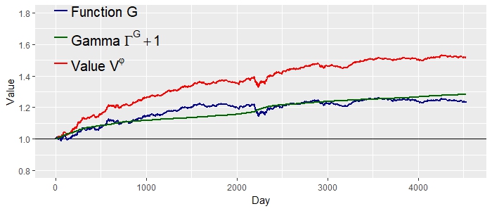
(a) Example 6.1
Original entropy, $p=9$

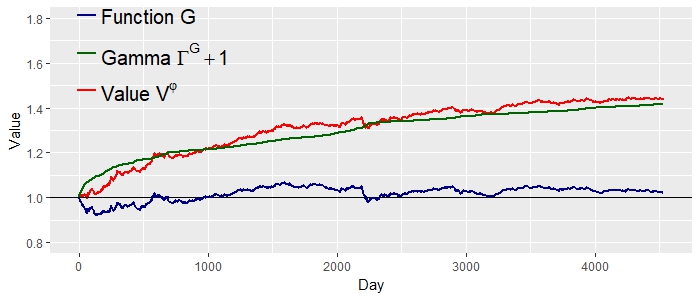
(b) Example 6.3
Entropy with running maximum, $p=9$

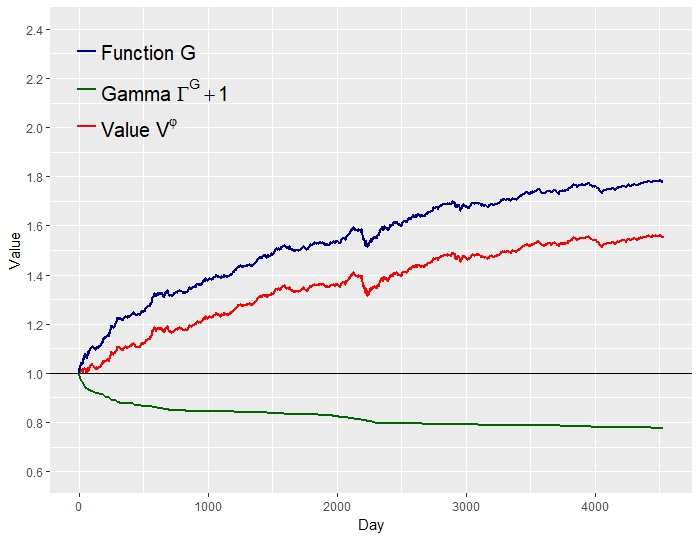
(c) Example 6.4
Entropy with running minimum, $p=9$

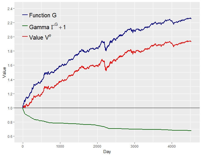
(d) Example 6.6
Iterated entropy with running minimum, $p=9$, $r=5$

Figure 1 confirms that all trading strategies additively generated in Section 6 outperform the market as the values $V^{\varphi}$ (red lines in the figure) gradually increase. In sub-figures (a) and (b), the growth of the value $V^{\varphi}$ comes from the growth of the Gamma function. In contrast, even though the Gamma function decreases, the value of trading strategy grows as the function $G$ increases substantially in sub-figures (c) and (d). In the sub-figure (d), we set the parameter $r=5$ as it is the largest integer satisfying the equation (6.27); initial market weights data give us $\max_{i}\mu_{i}(0)=0.065$ and $0.065<1/(5e)$ holds. We chose the same parameter $p=9$ (See Remark 6.2) in all sub-figures for fair comparison, but this is a very sloppy choice of the parameter $p$ for (a), (b), and (c). If we chose the value of $p$ using statistical estimation elaborately in each examples, the performance of portfolio would be improved, as Figure 2 represents in the case of Example 6.1.

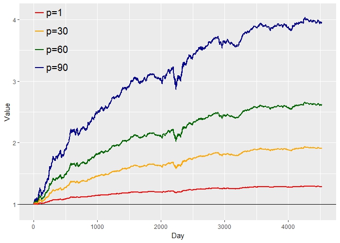
Figure 2: Value of additively generated trading strategies from Example 6.1 with different $p$ values

Figure 2 shows the values of additively generated portfolios in Example 6.1 with different choices of the parameter $p$. We can verify that trading strategy with bigger value of $p$ performs better as described in Remark 6.2. From the data, the Gibbs entropy $-\sum_{i=1}^{1085}\mu_{i}(t)\log\mu_{i}(t)$ of market weights ranged from $4.954$ to $5.726$ during 4528 days. Thus, $p=90$ is a safe estimation of the parameter $p$ which guarantees the non-negativity of the function $G$ in (6.2) as $\log 90<4.5<4.954$ holds.

Finally, ‘dollar values’ $W(\cdot)$ of portfolios from four examples of Section 6, which are defined as in (7.1), along with the total market value $\Sigma(\cdot)$ of $d=1085$ stocks from the start of 2000 to the end of 2017, are illustrated in Figure 3. Dollar values are normalized by replacing $W(\cdot)$ by $W(\cdot)/W(0)$. In Figure 3, while the market capitalization had been approximately doubled during $18$ years, the dollar values of all other portfolios had been grown more than $4.5$ times. Parameters are appropriately chosen using statistical estimation in each portfolio.

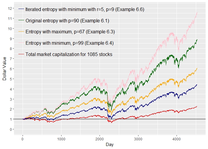
Figure 3: (Normalized) Dollar values of portfolios over 18 years

8 Conclusion

Karatzas and Ruf, (2017) introduced an alternative “additive” way of functional generation of trading strategies and compared it to the original “multiplicative” way of E.R. Fernholz. This new approach weakens the assumption on the asset prices from Itô processes to continuous semimartingales, characterizes the class of functions called “Lyapunov functions” which generate trading strategies leading to strong arbitrage with respect to the market, and gives a very simple sufficient condition for strong arbitrage. The present paper takes more generalized approaches to these two ways of functional generation. The results of this paper can be summarized as follows:

1. We show how to generate both additively and multiplicatively, trading strategies without any probabilistic assumptions on the market model. This is done by using the celebrated pathwise Itô calculus, and the only analytic assumption we impose is that the market weights admit continuous covariations in a pathwise sense. In the practical sense, we do not have to care about this analytic assumption because market weights data are given as the form of discrete time-series and such data always admit pathwise covariations.

2. We extend the class of functions which generate trading strategies by introducing an additional argument of finite variation other than market weights as the input. Inserting this argument in the generating function gives extra flexibility in portfolio construction and this has been dealt with in other literatures. However, we present some new examples of such extra argument which gives us simple sufficient condition leading to strong arbitrage relative to the market.

3. We also extend the class of functions which generate additive and multiplicative strong relative arbitrage by giving new sufficient conditions. The new conditions allow the function not be “Lyapunov”, or concave with respect to the market weights, in order to generate strong relative arbitrage or to outperform the market portfolio in the long run. We also present empirical results of portfolios which indeed outperform the market.

4. We further extend the class of portfolio-generating-functions from twice-differentiable to less smoother, namely absolutely continuous, functions with help of the pathwise Tanaka formula. Using Tanaka formula involves the concept of local times and this yields new interesting types of portfolios and corresponding strong arbitrage conditions.

While this paper generalizes the functional generation of portfolios in several respects, we suggest some new questions. First, this paper assumes a ‘closed market’, in other words, the number of stocks $d$ is fixed. In this respect, it fails to represent or resemble the real market. As explained in Remark 7.1, an ‘open market’ models the real world better, but nothing seems to be known on how to construct trading strategies in this open market. Secondly, the market weights in this paper should have finite second variation along a sequence of time partitions; can something be said, along the lives of Cont and Perkowski, (2018), regarding price dynamics, or market weights, with finite $p$-th variation for $p>2$?

Appendix A Proofs

Proof of Theorem 2.3.

Using the telescoping sum representation, we obtain

$$f\big{(}X(t),A(t)\big{)}-f\big{(}X(0)),A(0)\big{)} =\sum_{\begin{subarray}{c}[t_{j},t_{j+1}]\in\mathbb{T}_{n}\\ t_{j}\leq t\end{subarray}}\Big{\{}f\big{(}X(t_{j+1}),A(t_{j+1})\big{)}-f\big{(}X(t_{j}),A(t_{j})\big{)}\Big{\}}$$

$$=\sum_{\begin{subarray}{c}[t_{j},t_{j+1}]\in\mathbb{T}_{n}\\ t_{j}\leq t\end{subarray}}\Big{\{}f\big{(}X(t_{j+1}),A(t_{j+1})\big{)}-f\big{(}X(t_{j+1}),A(t_{j})\big{)}\Big{\}}$$ (A.1)

$$+\sum_{\begin{subarray}{c}[t_{j},t_{j+1}]\in\mathbb{T}_{n}\\ t_{j}\leq t\end{subarray}}\Big{\{}f\big{(}X(t_{j+1}),A(t_{j})\big{)}-f\big{(}X(t_{j}),A(t_{j})\big{)}\Big{\}}.$$ (A.2)

The Taylor expansion, applied to the components of the function $A$ in the sum (A.1), gives

$$~{}~{}~{}~{}~{}\sum_{\begin{subarray}{c}[t_{j},t_{j+1}]\in\mathbb{T}_{n}\\ t_{j}\leq t\end{subarray}}\Big{\{}f\big{(}X(t_{j+1}),A(t_{j+1})\big{)}-f\big{(}X(t_{j+1}),A(t_{j})\big{)}\Big{\}}$$ (A.3)

$$=\sum_{\begin{subarray}{c}[t_{j},t_{j+1}]\in\mathbb{T}_{n}\\ t_{j}\leq t\end{subarray}}\sum_{\ell=1}^{m}D_{\ell}f\big{(}X(t_{j+1}),A(t_{j})\big{)}\big{(}A_{\ell}(t_{j+1})-A_{\ell}(t_{j})\big{)}+\sum_{\begin{subarray}{c}[t_{j},t_{j+1}]\in\mathbb{T}_{n}\\ t_{j}\leq t\end{subarray}}\sum_{\ell=1}^{m}r\big{(}A_{\ell}(t_{j+1})-A_{\ell}(t_{j})\big{)},$$

where the last remainder term is bounded by

$$r\big{(}A_{\ell}(t_{j+1})-A_{\ell}(t_{j})\big{)}\leq\phi\Big{(}\max_{t_{j}}\big{|}A_{\ell}(t_{j+1})-A_{\ell}(t_{j})\big{|}\Big{)}\Big{|}A_{\ell}(t_{j+1})-A_{\ell}(t_{j})\Big{|}$$

for some function $\phi$ with the property $\lim_{x\rightarrow 0}\phi(x)=0$. Since $A$ is continuous and of bounded variation, the last double sum of the right-hand side of (A.3) goes to zero as $n\rightarrow\infty$ and the sum (A.1) converges to the Lebesgue-Stieltjes integral

$$\sum_{\ell=1}^{m}\int_{0}^{t}D_{\ell}f\big{(}X(s),A(s)\big{)}dA_{\ell}(s),$$

as $n\rightarrow\infty$. On the other hand, again by the Taylor expansion applied to the components of the function $X$ in the sum (A.2), we obtain

$$~{}~{}~{}~{}~{}\sum_{\begin{subarray}{c}[t_{j},t_{j+1}]\in\mathbb{T}_{n}\\ t_{j}\leq t\end{subarray}}\Big{\{}f\big{(}X(t_{j+1}),A(t_{j})\big{)}-f\big{(}X(t_{j}),A(t_{j})\big{)}\Big{\}}$$

$$=\sum_{\begin{subarray}{c}[t_{j},t_{j+1}]\in\mathbb{T}_{n}\\ t_{j}\leq t\end{subarray}}\sum_{i=1}^{d}\partial_{i}f\big{(}X(t_{j}),A(t_{j})\big{)}\big{(}X_{i}(t_{j+1})-X_{i}(t_{j})\big{)}$$ (A.4)

$$~{}~{}~{}+\frac{1}{2}\sum_{\begin{subarray}{c}[t_{j},t_{j+1}]\in\mathbb{T}_{n}\\ t_{j}\leq t\end{subarray}}\sum_{i,k=1}^{d}\partial^{2}_{i,k}f\big{(}X(t_{j}),A(t_{j})\big{)}\big{(}X_{i}(t_{j+1})-X_{i}(t_{j})\big{)}\big{(}X_{k}(t_{j+1})-X_{k}(t_{j})\big{)}$$ (A.5)

$$~{}~{}~{}+\sum_{\begin{subarray}{c}[t_{j},t_{j+1}]\in\mathbb{T}_{n}\\ t_{j}\leq t\end{subarray}}\sum_{i,k=1}^{d}r\big{(}X_{i,k}(t_{j+1})-X_{i,k}(t_{j})\big{)},$$ (A.6)

where the last remainder term (A.6) is bounded by

$$r\big{(}X_{i,k}(t_{j+1})-X_{i,k}(t_{j})\big{)}\leq\psi\Big{(}\max_{t_{j},i,k}\big{|}X_{i,k}(t_{j+1})-X_{i,k}(t_{j})\big{|}\Big{)}\big{(}X_{i}(t_{j+1})-X_{i}(t_{j})\big{)}\big{(}X_{k}(t_{j+1})-X_{k}(t_{j})\big{)},$$

for some function $\psi$ with the property $\lim_{x\rightarrow 0}\psi(x)=0$. Again, by the continuity of $X$ and by the fact that $X$ admits the pathwise quadratic covariation in the sense of (2.1), the double sum (A.6) approaches zero as $n\rightarrow\infty$. The sum (A.5) converges to the Lebesgue-Stieltjes integral

$$\frac{1}{2}\sum_{i,k=1}^{d}\int_{0}^{t}\partial^{2}_{i,k}f\big{(}X(s),A(s)\big{)}d\langle X_{i},X_{k}\rangle(s),$$

again by the existence of the pathwise quadratic covariation of $X$. As all the other terms converge, the remaining sum (A.4) should converge to some limit, which we call ‘Föllmer-Itô integral’ as in (2.5). ∎

Proof of Theorem 5.5.

For any two real numbers $a$ and $b$, by applying the integration by parts formula with the notation (5.4), we have the equation

$$f(b)-f(a) =\int_{a}^{b}f^{\prime}(x)dx$$

$$=\begin{cases}~{}~{}~{}\int_{a}^{b}f^{\prime}(x)(b-x)^{0}dx=-f^{\prime}(x)(b-x)\big{|}^{b}_{x=a}+\int_{(a,b]}(b-x)df^{\prime}(x),~{}\quad\text{if}~{}~{}~{}a\leq b\\ \\ -\int_{b}^{a}f^{\prime}(x)(b-x)^{0}dx=f^{\prime}(x)(b-x)\big{|}^{a}_{x=b}-\int_{(b,a]}(b-x)df^{\prime}(x),\qquad\text{if}~{}~{}~{}b<a\end{cases}$$

$$=\begin{cases}f^{\prime}(x)(b-a)+\int_{(a,b]}(b-x)df^{\prime}(x),\qquad\text{if}~{}~{}~{}a\leq b\\ \\ f^{\prime}(x)(b-a)-\int_{(b,a]}(b-x)df^{\prime}(x),\qquad\text{if}~{}~{}~{}b<a\end{cases}$$

$$=f^{\prime}(x)(b-a)+\int_{\mathbb{R}}\mathbbm{1}_{\llparenthesis a,b\rrbracket}(x)|b-x|df^{\prime}(x).$$ (A.7)

Thus, using the telescoping sum

$$f(X_{t})-f(X_{0})=\sum_{\begin{subarray}{c}[t_{j},t_{j+1}]\in\mathbb{T}_{n}\\ t_{j}\leq t\end{subarray}}\big{(}f(X_{t_{j+1}})-f(X_{t_{j}})\big{)}$$

for the sequence of partitions $\mathbb{T}=(\mathbb{T}_{n})_{n\in\mathbb{N}}$ of $[0,T]$, the above equality becomes

$$f(X_{t})-f(X_{0}) -\sum_{\begin{subarray}{c}[t_{j},t_{j+1}]\in\mathbb{T}_{n}\\ t_{j}\leq t\end{subarray}}f^{\prime}(X_{t_{j}})(X_{t_{j+1}}-X_{t_{j}})$$ (A.8)

$$=\sum_{\begin{subarray}{c}[t_{j},t_{j+1}]\in\mathbb{T}_{n}\\ t_{j}\leq t\end{subarray}}\int_{\mathbb{R}}\mathbbm{1}_{\llparenthesis X_{t_{j}},X_{t_{j+1}}\rrbracket}(x)|X_{t_{j+1}}-x|df^{\prime}(x)=\int_{\mathbb{R}}L_{t}^{X,\mathbb{T}_{n}}(x)df^{\prime}(x),$$

thanks to the definition (5.5). The last integral on the right-hand side of (A.8) converges to the last integral of (5.7), since $L_{t}^{X,\mathbb{T}_{n}}$ converges uniformly to $L_{t}$, and the result follows. ∎

References

- Cont, (2016) Cont, R. (2016). Functional Itô calculus and functional Kolmogorov equations. In Stochastic Integration by Parts and Functional Itô Calculus, pages 115–201. CRM Barcelona, Birkhäuser Basel.
- Cont and Perkowski, (2018) Cont, R. and Perkowski, N. (2018). Pathwise integration and change of variable formulas for continuous paths with arbitrary regularity. Preprint, arXiv:1803.09269v2, To appear in Transactions of the AMS.
- Davis et al., (2018) Davis, M., Obłój, J., and Siorpaes, P. (2018). Pathwise stochastic calculus with local times. Ann. Inst. H. Poincaré Probab. Statist., 54(1):1–21.
- Fernholz, (2002) Fernholz, E. R. (2002). Stochastic Portfolio Theory, volume 48 of Applications of Mathematics (New York). Springer-Verlag, New York. Stochastic Modelling and Applied Probability.
- Fernholz et al., (2018) Fernholz, E. R., Karatzas, I., and Ruf, J. (2018). Volatility and arbitrage. Ann. Appl. Probab., 28(1):378–417.
- Fernholz, (1999) Fernholz, R. (1999). Portfolio generating functions. In Avellaneda, M., editor, Quantitative Analysis in Financial Markets. World Scientific.
- Fernholz and Karatzas, (2009) Fernholz, R. and Karatzas, I. (2009). Stochastic Portfolio Theory: an overview. In Bensoussan, A., editor, Handbook of Numerical Analysis, volume Mathematical Modeling and Numerical Methods in Finance. Elsevier.
- Föllmer, (1981) Föllmer, H. (1981). Calcul d’Itô sans probabilités. In Séminaire de Probabilités, XV (Lecture Notes in Mathematics, Volume 850), pages 143–150. Springer-Verlag, Berlin.
- Karatzas and Ruf, (2017) Karatzas, I. and Ruf, J. (2017). Trading strategies generated by Lyapunov functions. Finance and Stochastics, 21(3):753–787.
- Perkowski and Prömel, (2015) Perkowski, N. and Prömel, D. (2015). Local times for typical price paths and pathwise Tanaka formulas. Electron. J. Probab., 20:15 pp.
- Ruf and Xie, (2018) Ruf, J. and Xie, K. (2018). Generalised Lyapunov functions and functionally generated trading strategies. Preprint, arXiv:1801.07817v1.
- Schied et al., (2018) Schied, A., Speiser, L., and Voloshchenko, I. (2018). Model-free portfolio theory and its functional master formula. SIAM Journal on Financial Mathematics, 9(3):1074–1101.
- Strong, (2014) Strong, W. (2014). Generalizations of functionally generated portfolios with applications to statistical arbitrage. SIAM Journal on Financial Mathematics, 5(1):472–492.
- Wuermli, (1980) Wuermli, M. (1980). Lokalzeiten für Martingale. Diploma thesis, Universität Bonn.