Quantum Chameleons

Abstract

We initiate a quantum treatment of chameleon-like particles, deriving classical and quantum forces directly from the path integral. It is found that the quantum force can potentially dominate the classical one by many orders of magnitude. We calculate the quantum chameleon pressure between infinite plates, which is found to interpolate between the Casimir and the integrated Casimir-Polder pressures, respectively in the limits of full screening and no screening. To this end we calculate the chameleon propagator in the presence of an arbitrary number of one-dimensional layers of material. For the Eöt-Wash experiment, the five-layer propagator is used to take into account the intermediate shielding sheet, and it is found that the presence of the sheet enhances the quantum pressure by two orders of magnitude. As an example of implication, we show that in both the standard chameleon and symmetron models, large and previously unconstrained regions of the parameter space are excluded once the quantum pressure is taken into account.

I Introduction

A wealth of Dark Energy models involve a scalar field with an extremely low mass which plays a role on cosmological scales Brax (2013), explaining the accelerated expansion of the Universe. At shorter distances, such as the Solar System scale, screening mechanisms must take place to suppress the long-range force induced by the new scalar, since such scenario would be otherwise excluded by stringent experimental tests Bertotti et al. (2003); Williams et al. (2012). Screening mechanisms of the long-range force can naturally occur as a result of the scalar coupling to matter. Indeed, whenever the local matter density is high enough with respect to the other scales of the problem, the properties of the scalar (mass or couplings) tend to change in the local environment and, typically, the scalar tends to get invisible where one could observe it Khoury and Weltman (2004a, b); Brax et al. (2004a, 2010a). We will refer to any scalar with such property as a chameleon-like field (and will sometimes use only “chameleon” for short). For instance for the original chameleon model the mass of the field increases in dense environments whilst in the symmetron model Pietroni (2005); Olive and Pospelov (2008); Hinterbichler and Khoury (2010) screening occurs as the coupling to matter decreases with an increasing matter density. The existence of chameleon-like fields can be tested by laboratory experiments, for instance by neutrons Brax and Pignol (2011); Jenke et al. (2014); Lemmel et al. (2015); Cronenberg et al. (2018) or atomic spectroscopy Burrage and Copeland (2016); Jaffe et al. (2017). The pressure between two parallel plates is also suited to test the potential presence of chameleons Brax et al. (2007, 2010b) which could become within reach in the near future Almasi et al. (2015).

The effects of chameleon-like fields are typically treated in a classical approximation. However at short enough distances – such as the submicron scale in the Eöt-Wash experiment Adelberger et al. (2007), a quantum treatment of the chameleon mechanism becomes mandatory. In this work we develop the formalism to describe “quantum chameleons” and present some of its consequences. The formalism also sheds new light on the quantum field theory calculation of the Casimir pressure in its various regimes, providing for instance the general quantum pressure interpolating between the Casimir and the Casimir-Polder limits.

The paper is arranged as follows. In section II we calculate the force between bodies due to a chameleon-like field at the classical and quantum levels. In section III we restrict ourselves to the quantum chameleon force between parallel plates. We then apply our results to obtain constraints from fifth force experiments in section IV. We conclude in Sec. VI and more details on the Feynman propagators and the Casimir-Polder force are given in the Appendix.

II Chameleon forces from the path integral

Our focus in this work is on scalar-tensor theories with a conformal coupling between the scalar field and matter Damour and Esposito-Farese (1992). In the Einstein frame this translates into the general chameleon Lagrangian

$${\cal L}[\phi,J]=\frac{1}{2}(\partial_{\mu}\phi)^{2}-V(\phi)-A(\phi)J\,,$$ (1)

where gravity is described by its Einstein-Hilbert Lagrangian, $V(\phi)$ is the interaction potential of the scalar field, and $J$ is a source representing the density of pressure-less matter in the setting. The term $A(\phi)J$ describes how the chameleon couples to the source . In this works the source $J$ is considered as a matter density, i.e. $J(x)=\rho(x)$, which is assumed to be static and vanishes at infinity. In general $J$, $\phi$, $A(\phi)$ depend on space. Both $V$ and $A$ can contain higher dimensional operators, in which case the Lagrangian describes a low-energy effective field theory (EFT) valid for distances greater than some UV cutoff scale. In the following we define the effective potential

$$V_{J}=V+AJ\,.$$ (2)

The source is assumed to depend on an external parameter $L$, to be understood typically as measuring the distance between two objects, $L=|L^{i}|$. Our goal is to study how the quantum system reacts when changing $L$.

We are interested in calculating the energy of a configuration involving several objects acting as sources, all described by the distribution $J$. The energy involves both the classical energy due to the classical field configuration between the bodies and the quantum fluctuations around the classical value. The energy of the set of objects can be obtained by integrating over the scalar field. This can be performed using a path integral $Z[J]$ whose source term is the $J$ distribution representing the objects. The relevant information is contained in the generating functional of connected correlators, given by

$$W[J]=i\log Z[J]\,,\quad Z[J]=\int{\cal D}\phi e^{i\int d^{4}x{\cal L}[\phi,J]}\,.$$ (3)

This is the Lorentzian analog to the free-energy in Euclidian space (see e.g Peskin and Schroeder (1995)). When the source is static, $W[J]$ involves only a potential energy which is given by

$$E[J]=\frac{W[J]}{T}\,$$ (4)

where $T=\int dt$ is the integral over time. We will work with $T=1$ conventionally and refer to the potential $E[J]$ as the vacuum energy. Our conventions regarding spacetime coordinates are $x^{\mu}=(t,x^{i})$, $d^{4}x\equiv dtd^{3}x$, $d^{3}x\equiv dx^{1}dx^{2}dx^{3}$.

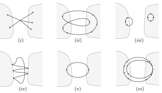
Figure 1: Sample Feynman diagrams for a chameleon field in the presence of two extended sources. (i): A generic classical contribution. (ii): A generic 1-loop contribution. (iii): Tadpoles. (iv): Casimir (Strong coupling to sources.) (v):Casimir-Polder (Weak coupling to sources.) (vi): A two-loop contribution from higher-dimensional coupling to matter.

All the information about the force (or pressure) that one source induces on another one in the presence of the chameleon-like field is contained in the variation of the vacuum energy with respect to $L$. This variation is given by

$$\partial_{L}E[J]=\frac{\int{\cal D}\phi\int d^{3}x\partial_{L}JA(\phi)e^{i\int d^{4}x{\cal L}[\phi,J]}}{\int{\cal D}\phi e^{i\int d^{4}x{\cal L}[\phi,J]}}\,.$$ (5)

As the numerator is simply a normalising constant, this can be rewritten as

$$\partial_{L}E[J]=\int d^{3}x\,\partial_{L}J\left(\frac{\int{\cal D}\phi A(\phi)e^{i\int d^{4}x{\cal L}[\phi,J]}}{\int{\cal D}\phi e^{i\int d^{4}x{\cal L}[\phi,J]}}\right)$$ (6)

where we have commuted the integrals and extracted the factor $\int d^{3}x\,\partial_{L}J$ from the functional integral as this is a field independent term. The term in brackets can be seen as the averaged value of $A$ over all the field configurations of $\phi$, leading to the general expression for the force

$$\partial_{L}E[J]=\int d^{3}x\,\partial_{L}J\,\langle A\rangle_{J}\,,$$ (7)

where

$$\langle A\rangle_{J}=\frac{\int{\cal D}\phi A(\phi)e^{i\int d^{4}x{\cal L}[\phi,J]}}{\int{\cal D}\phi e^{i\int d^{4}x{\cal L}[\phi,J]}}$$ (8)

depends on the sources $J$.

Notice that in the functional integral defining $E[J]$, only the source term depends on $L$ and therefore the variation with respect to $L$ is only operative on the source $J$. This is the reason why the variation of the vacuum energy Eq. (7) only involves $\partial_{L}J$. From a functional derivative viewpoint, $\langle A\rangle_{J}$ is given by $\langle A\rangle_{J}=\delta E[J]/\delta J$, i.e. Eq. (7) is simply an elaborate version of the chain rule. Namely, the formula decouples the quantum average leading to $\langle A\rangle_{J}\$ and the change in the positions of the bodies captured by $\partial_{L}J$. In a sense, Eq. (7) is deceptively simple as the calculation of the quantum average $\langle A\rangle_{J}$ is highly non-trivial and can in general be evaluated only in the loop expansion of quantum field theory.

To go further, let us thus perform the $\hbar$ expansion. Writing the chameleon field as $\phi=\phi_{\rm cl}+\eta$ where $\eta$ represents the quantum fluctuations around the classical field $\phi_{\rm cl}$, we find the first two terms in the $\hbar$ expansion to be

$$\partial_{L}E =\int d^{3}x\partial_{L}JA(\phi_{\rm cl})+\frac{1}{2}\int d^{3}x\partial_{L}JA^{\prime\prime}\Delta_{J}(x,x)+O(\hbar^{2})$$

$$=F_{\rm cl}+F_{\rm quant}+O(\hbar^{2})\,,$$ (9)

where $\Delta_{J}(x,x^{\prime})$ is the Feynman propagator of the fluctuation, which satisfies the equation of motion

$$(\partial^{2}_{x}+V^{\prime\prime}+A^{\prime\prime}J)\Delta_{J}(x,x^{\prime})=-i\delta^{(4)}(x-x^{\prime})\,,$$ (10)

where $V^{\prime\prime}=\frac{d^{2}V}{d\phi^{2}}|_{\phi=\phi_{\rm cl}}$, $A^{\prime\prime}=\frac{d^{2}A}{d\phi^{2}}|_{\phi=\phi_{\rm cl}}$. The convention adopted here is that $F>0$ for an attractive force. The Feynman prescription will be specified below and in appendix B. An efficient way to obtain the general result Eq. (9) is to expand $\phi$ in Eq. (8), which gives $\langle A(\phi)\rangle=A(\phi_{\rm cl})+\frac{1}{2}A^{\prime\prime}(\phi_{\rm cl})\langle\eta(x)^{2}\rangle+O(\hbar^{2})$, and realise that $\langle\eta(x)^{2}\rangle$ is the connected correlator of $\eta$ in presence of the source term, i.e. $\Delta_{J}(x,x)$. A more pedestrian derivation using the 1-loop functional determinant will be described further below and in App. A.

The first term in Eq. (9) is the classical force, pictured in Fig. 1i. This term does not involve relativistic retardation and only requires to solve the background equation of motion. When for instance $A(\phi)=y\phi$, $V(\phi)=\frac{1}{2}m^{2}\phi^{2}$, one recovers exactly the Yukawa force (note one can use $\langle\phi\rangle(x)=y\int d^{4}x^{\prime}i\Delta(x,x^{\prime})J(x^{\prime})$) giving the same result as in Brax and Davis (2015).

One can also notice that when writing explicitly the source as describing two bodies $a$ and $b$ in the form $J(x^{i})=J_{a}(x^{i}-L^{i})+J_{b}(x^{i})$, using $\partial_{L^{i}}J_{a}=-\partial_{i}J_{a}$, and using the fact that the bodies vanish at infinity, we obtain

$$F_{i}=\int d^{3}x\,\rho_{a}(x^{i})\partial_{i}A(\phi_{\rm cl})\,$$ (11)

after integrating by part. This matches the classical result used in Brax and Davis (2015) and used to calculate classical forces in scalar-tensor theories.

The second term in Eq. (9) is the quantum force at one-loop order, pictured in Fig. 1ii. One method to obtain it is to use the explicit evaluation of $E[J]$, which contains the 1-loop functional determinant (see e.g Peskin and Schroeder (1995))

$$E[J] \supset-\frac{i}{2}{\rm Tr}\log(\partial^{2}+V^{\prime\prime}+A^{\prime\prime}J)$$ (12)

$$=\frac{i}{2}\left(\sum_{n=1}^{\infty}\frac{1}{n}{\rm Tr}\left(-\frac{A^{\prime\prime}J}{\partial^{2}+V^{\prime\prime}}\right)^{n}-{\rm Tr}\log(\partial^{2}+V^{\prime\prime})\right).$$

The variation of $E[J]$ with respect to $L$ is detailed in App. A and gives

$$\partial_{L}E[J]\supset\frac{i}{2}\int d^{3}xA^{\prime\prime}\partial_{L}J(-i)\Delta_{J}(x,x)+O(\hbar^{2})$$ (13)

where the quantity

$$\Delta_{J}(x,x^{\prime})=-i(\partial^{2}+V^{\prime\prime})^{-1}\sum_{n=0}^{\infty}{\rm Tr}\left(-\frac{A^{\prime\prime}J}{\partial^{2}+V^{\prime\prime}}\right)^{n}$$ (14)

has appeared, which is precisely the geometric series representation of $\Delta_{J}$ satisfying Eq. (10). The result Eq. (13) reproduces the quantum force formula given in Eq. (9).

The vacuum energy (in)famously contains infinities which usually have to be subtracted by hand (see e.g. Weinberg (1989); Milton (2003)). In our approach all divergences automatically disappear thanks to the $\partial_{L}$ as they are $L$-independent, as should be the case as $\partial_{L}E[J]$ is an observable. Indeed, in the functional determinant, the $\partial_{L}$ removes all diagrams which do not link a source to the other one, i.e. the “tadpole” diagrams of the extended sources, pictured in Fig. 1iii. Thus in Eq. (9) the infinite part of $\Delta(x,x)$ (which is $L$-independent) does not contribute and one can readily use its finite part $\Delta^{\rm fin}(x,x)$. More details are given in App. B.

II.1 An aside: Boundary integral representation

Before discussing further the properties of the chameleon quantum force, it is worth pointing out another representation which applies to the general force Eq. (9), or to any of the term of the $\hbar$ expansion separately. The following formalism applies to bodies with sharp boundaries, whose volumes $V_{a,b}$ can be described in the form

$$f_{a}(x^{i}-L^{i})\geq 0\,,\quad f_{b}(x^{i})\geq 0\,.$$ (15)

The source $a$ can generically be modeled as

$$J_{a}(x^{i})=\rho_{a}(x^{i})\Theta(f_{a}(x^{i}-L^{i}))$$ (16)

with a space-varying density $\rho_{a}(x^{i})$, and similarly for $b$. Such modeling of the sources applies to essentially all physically relevant situations.

Let us remark that the variation of source $a$ with respect to $L^{i}$ gives

$$\partial_{L^{i}}J_{a}=-\rho_{a}(x^{i})\partial_{i}f_{a}(x^{i}-L^{i})\delta(f_{a}(x^{i}-L^{i}))\,.$$ (17)

Using Eq. (17), the force is given by an integral over the boundary $S$ of $V_{a}$. Parametrizing the boundary manifold using coordinates $\xi_{\alpha}$ $(\alpha=1,2)$ with induced metric $g_{\alpha\beta}$, we have

$$F^{i}=-\int_{S}d^{2}\xi\sqrt{g}\,n^{i}\,\rho(x^{i})\langle A\rangle_{J}$$ (18)

where

$$n^{i}=\frac{\partial_{i}f_{a}(x^{i}-L^{i})}{|\partial_{i}f_{a}(x^{i}-L^{i})|}\,$$ (19)

is the unit vector normal to $S$ and oriented inwards $V_{a}$.

To study the modulus of the force, let us chose a coordinate system such that $L^{i}=(0,0,L^{z})$ without loss of generality. In these coordinates the force modulus is given by

$$|F|=F^{z}=-\int_{S}d^{2}\xi\sqrt{g}\,n^{z}\,\rho(x^{i})\langle A\rangle_{J}$$ (20)

Since the volume is closed, $n^{z}$ can take both signs. This naturally splits the integral into a positive contribution from $S_{+}=(\xi^{\alpha}|n^{z}\geq 0)$ and a negative contribution from $S_{-}=(\xi^{\alpha}|n^{z}<0)$. The presence of these two opposite-sign contributions in the boundary integral is helpful to understand how infinite contributions cancel in the quantum case. This will be explicitly illustrated in the case of plates in Sec. III.

II.2 The chameleon quantum force

Computing the quantum force (Eq. (9)) requires to calculate the $\Delta_{J}$ propagator. However some important general properties can be deduced prior to any calculation. Whenever the source term $A^{\prime\prime}J$ is large with respect to other scales involved in the interaction potential, the Green’s function should vanish (i.e. be “screened”) inside the source and vanish at its surface, as illustrated in Fig. 1iv, see appendix B. These are precisely the conditions for the standard Casimir effect.

In the opposite limit, when the coupling to the source $A^{\prime\prime}J$ can be treated perturbatively, the functional determinant Eq. (12) can be truncated at quadratic order, in which case it is the limit of no screening where the force is

$$F_{\rm quant}= \frac{i}{2}\int d^{3}x\int d^{4}x^{\prime}$$ (21)

$$A^{\prime\prime}(x)\partial_{L}J(x)\Delta_{0}(x,x^{\prime})A^{\prime\prime}(x^{\prime})J(x^{\prime})\Delta_{0}(x^{\prime},x)\,.$$

This corresponds to the bubble diagram shown in Fig. 1v, which is precisely the Casimir-Polder force integrated over extended sources, see appendix E. For point sources $J(x)=\delta^{(3)}(x^{i})+\delta^{(3)}(x^{i}-L^{i})$, $|L^{i}|=L$, we obtain the potential

$$V_{\rm CP}(L)=-A^{\prime\prime}(0)A^{\prime\prime}(L)\frac{1}{32\pi^{3}}\frac{V^{\prime\prime}}{L^{2}}K_{1}(2V^{\prime\prime}L)\,.$$ (22)

This is a generalisation of the Casimir-Polder potential in the presence of an unscreened scalar, which matches results of Refs. Fichet (2018); Brax et al. (2018a) when taking $A(\phi)=\frac{\phi^{2}}{2M}$ and $V(\phi)=\frac{m^{2}}{2}\phi^{2}$.

The chameleon-like models are effective theories whose predictions are valid below a cutoff scale, specific to each experimental situation. When self-interactions such as ${\cal L}\supset\phi^{n}/\Lambda^{n-4}$ are present, the cutoff is expected to be $\sim 4\pi\Lambda$ since higher order diagrams are expected to produce fast-growing $1/(\Lambda L)^{n}$ contributions to the force which cannot be neglected when $L\sim 1/4\pi\Lambda$. The cutoff resulting from the interactions with matter is more subtle because of screening. Consider the contributions to the force from the leading interaction $M^{-2}\phi^{2}J$ and a next-to-leading interaction of order $M^{-4}\phi^{4}J$ (shown in Fig. 1vi), which contributes at two-loop as

$${\rm 2-loop}\sim M^{-2}\int d^{3}x\partial_{L}J(\Delta(x,x))^{2}\,.$$ (23)

We obtain that the two loop contribution is negligible for 

$$\Delta^{\rm fin}_{J}(x_{bd},x_{bd})\ll M^{2}\,.$$ (24)

In the presence of screening, one has

$$\Delta^{\rm fin}_{J}(x_{bd},x_{bd})\rightarrow 0\,,$$ (25)

see appendix B, and therefore the range of validity of the calculation of the quantum force is largely extended. This is not surprising as the Casimir pressure should not depend on the coupling to the plates, only on the mass and degrees of freedom of the field living between the plates. Also, this screening is a familiar effect in compact extra-dimension theories Brax et al. (2004b): a large brane mass term repels the field and amounts to a Dirichlet boundary condition Carena et al. (2002, 2003). Yet, it is remarkable that the presence of screening reduces the contributions from $n>1-$loop diagrams, hence improving on the $\hbar$ expansion.

Our conclusions about the validity of the chameleon-like EFT differ from those drawn in Ref. Upadhye et al. (2012) for the following reason. The reasoning of Ref. Upadhye et al. (2012) would hold if the source occupied the whole space. However one should take into account that whenever an empty region exists, the fluctuation gets confined there when the effective mass induced by the source becomes large (as pictured in Fig. 1iv). As a consequence the contributions to the $1-$loop potential in the source region are suppressed by the vanishing wave function of the fluctuation, and the chameleon-like EFT is not violated—even when the effective mass induced by the source becomes infinite.

III Quantum force between plates

We now study the case of a chameleon-like field in an environment whose constant density changes piece-wise along the direction $z$. We construct configurations with two facing plates, by first taking the plates to be of finite width to guarantee that the density vanishes at infinity and then taking the limit of infinite width.

The classical component of the chameleon force in this geometry has been extensively studied. It can be obtained using for instance Eq. (11) or Eq. (18), which gives $F_{\rm cl}/S=\rho_{3}|A(L)-A(\infty)|$, and can be further transformed to

$$\frac{F_{\rm cl}}{S}=|V_{J}(\phi_{\rm vac})-V_{J}(\phi_{0})|$$ (26)

where $\phi_{\rm vac}$ is the values of the field in the absence of the plates and $\phi_{0}$ is the value of the field midway between the plates, see Brax and Davis (2015). We will recall the expressions of the classical pressure for inverse power-law chameleons Khoury and Weltman (2004a) and symmetrons Hinterbichler and Khoury (2010) in the next sections. The present section is about the quantum component force.

We model the mass of the chameleon fluctuation as a piecewise constant along $z$. This piecewise mass model is important as it is a sensible approximation whenever the profile of $\phi_{\rm cl}$ near the interfaces is irrelevant compared the distance $L$. This piecewise constant mass approximation is especially accurate for symmetron models Brax and Pitschmann (2018).

Let us then consider three regions, for which the effective mass $V_{J}^{\prime\prime}\equiv m^{2}(z)$ takes the form

$$m^{2}(z)=m_{1}^{2} \Theta(-z_{\infty}<z<0)+m_{2}^{2}\Theta(0<z<L)$$

$$+m_{3}^{2}\Theta(L<z<z_{\infty})\,,$$ (27)

where $|z_{\infty}|$ is near infinity, i.e. larger than all other length scales of the problem. This model can be readily used to calculate the chameleon pressure between plates of homogeneous mass density $\rho$, in which case $m_{2}^{2}$ is seen as the intrinsic mass and the sources in regions 1, 3 are identified with $M^{-2}J_{1,3}=(M)^{-2}\,\rho_{1,3}=m^{2}_{1,3}-m_{2}^{2}$.

Defining $\omega(z)=\sqrt{(p_{0})^{2}-(p_{1})^{2}-(p_{2})^{2}+i\epsilon-m^{2}(z)}$, the equation of motion becomes

$$(\partial_{z}^{2}+\omega^{2}(z))\phi(z)=0\,.$$ (28)

The solution in regions $i=1,2,3$ is simply $(\phi_{i}^{+},\phi_{i}^{-})=(e^{i\omega_{i}z},e^{-i\omega_{i}z})$. The solution everywhere can be found by continuity of the solution and its derivative at each of the interfaces, defining momentum-dependent transfer matrices of the form

$$(\phi_{2}^{+},\phi_{2}^{-})^{t}=T_{21}(\phi_{1}^{+},\phi_{1}^{-})^{t}\,,\quad(\phi_{3}^{+},\phi_{3}^{-})^{t}=T_{32}T_{21}(\phi_{1}^{+},\phi_{1}^{-})^{t}\,.$$ (29)

More details about the propagator are given in the Appendices B, which also includes details about the Feynman prescription and analytic continuation.

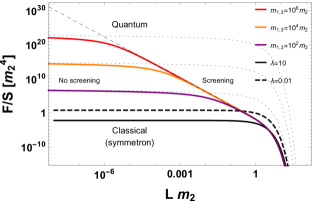
Figure 2: Top: The quantum pressure between plates as a function of $L$ for fixed $m_{2}$ (or vice-versa). Thin dashed line shows the Casimir pressure for a massive scalar. Thin dotted lines show the integrated Casimir-Polder force. The exact result interpolates between these two regimes. The classical pressure in the symmetron model where $m^{2}_{2}=2\mu^{2}$ is also shown. Bottom: Lower bound on $ML$ needed for the perturbative expansion to be valid.

The quantum force induced by the fluctuation between regions 1 and 3 is obtained by varying $E[J]$ with respect to $L$, as described in Eq. (9). The variation of the source gives $A^{\prime\prime}\partial_{L}J=(m_{2}^{2}-m_{3}^{2})\left(\delta(z-L)-\delta(z-z_{\infty})\right)$. This makes appear the quantity $\Delta_{p}(L,L)-\Delta_{p}(z_{\infty},z_{\infty})\equiv\Delta^{\rm fin}_{p}(L,L)$, where

$$\Delta_{p}(L,L)=\frac{(\omega_{1}+\omega_{2})+e^{2iL\omega_{2}}(\omega_{2}-\omega_{1})}{(\omega_{1}+\omega_{2})(\omega_{2}+\omega_{3})-e^{2iL\omega_{2}}(\omega_{2}-\omega_{1})(\omega_{2}-\omega_{3})}\,$$ (30)

and $\Delta_{p}(z_{\infty},z_{\infty})=1/(\omega_{2}+\omega_{3})$. The final expression for the pressure between regions $1$ and $3$ is then

$$\frac{F_{\rm quant}}{S}=\int_{0}^{\infty}\frac{d\rho\rho^{2}}{2\pi^{2}}$$ (31)

$$\frac{\gamma_{2}(\gamma_{2}-\gamma_{1})(\gamma_{2}-\gamma_{3})}{e^{2L\gamma_{2}}(\gamma_{1}+\gamma_{2})(\gamma_{2}+\gamma_{3})-(\gamma_{2}-\gamma_{1})(\gamma_{2}-\gamma_{3})}\,\,$$

where one has performed a Wick rotation and introduced $\omega_{i}=i\gamma_{i}=i\sqrt{\rho^{2}+m^{2}_{i}}$.

Let us consider some limiting cases. For $m_{1,3}\rightarrow\infty$, the expression gives the Casimir pressure from a massive scalar,

$$\frac{F_{\rm quant}}{S}=\int_{0}^{\infty}\frac{d\rho\rho^{2}}{2\pi^{2}}\frac{\gamma_{2}}{e^{2L\gamma_{2}}-1}\,\,$$ (32)

which is $\pi^{2}/(480L^{4})$ if $m_{2}=0$.

On the other hand, weak coupling is defined by $(m^{2}_{1,3}-m_{2}^{2})/m^{2}_{2}\ll 1$ in which case a perturbative expansion is possible. The leading order in the expansion is quadratic and gives

$$\frac{F_{\rm quant}}{S}=(m^{2}_{1}-m_{2}^{2})(m^{2}_{3}-m_{2}^{2})\int_{0}^{\infty}\frac{d\rho\rho^{2}}{2\pi^{2}}\frac{e^{-2L\gamma_{2}}}{16(\gamma_{2})^{3}}\,.$$ (33)

This corresponds exactly to the Casimir-Polder force integrated over regions 1 and 3.

Although the limits taken above are conceptually simple, the transition between both as a function of $L$ is non trivial, as shown in Fig. 2. We see that the transition occurs over 3 orders of magnitude in $L$ and takes place near $L\sim 1/m_{1,3}$. Qualitatively, this is the typical distance for which the chameleon-like fluctuation has high enough momentum to start travelling in the $1,3$ regions. This behaviour can be seen as a validity cutoff on the Casimir pressure, in the sense that at close enough distance the pressure becomes constant instead of keeping growing. This behaviour can be see in Fig. 2 at low values of $L$. An $O(1)$ estimate of the pressure in this regime, taking $m_{1}\sim m_{3}$, is given by

$$\frac{F_{\rm quant}}{S}\sim-\frac{(m^{2}_{1}-m_{2}^{2})(m^{2}_{3}-m_{2}^{2})}{32\pi^{2}}\log m_{1,3}L\,,$$ (34)

and applies both for $m_{1,3}\gg m_{2}$ (strong coupling) and $m_{1,3}\sim m_{2}$ (weak coupling).

The validity cutoff of the prediction of the quantum force in the presence of a higher-dimensional coupling to matter is shown in Fig. 2. The minimum value allowed for $ML$, defined as $(ML)_{\rm val}\equiv L\sqrt{\Delta^{\rm fin}_{J}(x_{\rm bd},x_{\rm bd})}$ following Eq. (24), reaches a maximal value of $\sim 0.02$, which is similar to $\sim 1/4\pi$. This corresponds to the lowest possible scale $M$ for a given $L$. Conversely, for a given $M$ this gives the domain of validity of the EFT as a function of $L$. In the screening limit $m_{1,3}\gg 1/L$ the range of validity is largely widened. We have that $\Delta^{\rm fin}_{J}(x_{\rm bd},x_{\rm bd})\simeq\frac{\pi^{2}}{480m_{1,3}^{2}L^{4}}$ hence the EFT validity condition Eq. (24) takes the simple form

$$L\gg\frac{1}{\sqrt{Mm_{1,3}}}\,$$ (35)

which goes to much shorter length scales than $1/4\pi M$ .

IV Quantum force in the Eöt-Wash experiment

The torsion pendulum Eöt-Wash experiment involves two plates separated by a distance $L$ in which holes have been drilled regularly on a circle. The two plates rotate with respect to each other. The scalar interaction induce a torque on the plates which depends on the potential energy of the configuration. The potential energy is obtained by calculating the amount of work required to approach one plate from infinity Brax et al. (2008); Upadhye (2012). Defining by $S(\theta)$ the surface area of the two plates which face each other at any given time, the torque is obtained as the derivative of the potential energy of the configuration with respect to the rotation angle $\theta$ and is given by

$$T\sim a_{\theta}\int_{L}^{\infty}dx\;\frac{F}{S}(x)\,,$$ (36)

where $a_{\theta}=\frac{dS}{d\theta}$ depends on the experiment. For the 2006 Eöt-Wash experiment Kapner et al. (2007), we consider the bound obtained for a separation between the plates of $D=55\mu{\rm m}$,

$$|T|\leq a_{\theta}\Lambda_{T}^{3},$$ (37)

where $\Lambda_{T}=0.35\Lambda$ Brax et al. (2008) where $\Lambda\sim 2.4$ meV is the dark energy scale. Importantly, a thin electrostatic shielding sheet is placed between the plates. It turns out that the presence of this sheet modifies both the classical and quantum components of the torque induced by the putative chameleon field, as we will see in the following.

The Eöt-Wash experiment is sensitive to many modified gravity models, it is thus interesting to evaluate the quantum force from a chameleon-like field in this setup. We use, as above, the piecewise constant mass approximation for the chameleon-like fluctuations. Because of the electrostatic shielding sheet present between the plates, the chameleon particle propagates in 5 different regions. The 5-layer propagator is obtained using the method described in Sec. III, and the subsequent change in force is shown in Fig. 3 for a massless particle. We see that when the sheet is dense enough, it screens the propagation and the quantum force is enhanced by a factor 16, as the pressure is now between the plate and the sheet, twice closer than the opposite plate. The full expression for the force in 5 regions is heavy and not very illuminating. But in the screening limit of the sheet the Casimir pressure is found to be $\pi^{2}/(30(L-W_{\rm sheet})^{4})$, where $W_{\rm sheet}$ is the width of the sheet ($L=55$ $\mu$m, $W_{\rm sheet}=10$ $\mu$m for Adelberger et al. (2007)).

Interestingly, without the sheet, the $L=55$ $\mu$m Eöt-Wash measurement is already close to be sensitive to the Casimir pressure induced by a chameleon-like particle. Once the effect of the sheet is taken into account, the pressure is enhanced and Eöt-Wash then becomes sensitive to the chameleon Casimir pressure.

V Quantum bounds on chameleon-like models

Here we consider the implications of the previous results for two well-known models for which the piecewise constant mass approximation can be safely used. In each model we first define the masses $m_{i}$ and give the classical force. The quantum force is obtained using the formalism developed in this paper.

Standard chameleon. The standard chameleon potential is

$$V_{J}(\phi)=\frac{\Lambda^{4+n}}{\phi^{n}}+e^{\frac{\phi}{M}}J\,.$$ (38)

and has been studied in great details Burrage and Sakstein (2016); Brax et al. (2018b). The mass between the plates is given by

$$m_{2}L\approx\sqrt{\frac{2(n+1)}{n}}B\left(\frac{1}{2},\frac{1}{2}+\frac{1}{n}\right)$$ (39)

where $B$ is the Euler function. This is true as long as $L\gg m_{1,3}^{-1}$ where the masses in the plates are $m_{1,3}^{2}=\Lambda^{n+4}/\phi_{1,3}^{n+2}$ and the fields in the plates are given by $\phi_{1,3}^{n+1}=n\Lambda^{n+4}MJ_{1,3}$. The classical Casimir pressure is then

$$\frac{F_{\rm cl}}{S}\approx\Lambda^{4}\left(\frac{\sqrt{2}n}{B(\frac{1}{2},\frac{1}{2}+\frac{1}{n})}\Lambda L\right)^{-2n/(n+2)}$$ (40)

which is a power law as a function of $L$.

Focussing on $n=1$, the chameleon mass between the plates is $m_{2}\approx\pi/L$. We find that the most precise Casimir force experiments Bordag (2009); Decca et al. (2007a, b) are sensitive to the small extra Casimir pressure induced by the chameleon. It turns out that exclusions from classical and quantum forces are complementary, and the quantum force excludes a large region inaccessible to other experiments, as shown in Fig. 3.

Symmetron. The symmetron model relies on the restoration of a $Z_{2}$ symmetry in the presence of matter and is usually realised as

$$V_{J}(\phi)=\frac{1}{2}\left(\frac{1}{M^{2}}J-\mu^{2}\right)\phi^{2}+\frac{\lambda}{4}\phi^{4}\,.$$ (41)

When $J>\mu^{2}M^{2}$ the expected value of the field is $\phi_{\rm cl}=0$ and the mass of the fluctuation is $\sqrt{M^{-2}J-\mu^{2}}$ whilst for smaller densities the field is $\phi_{\rm cl}=\frac{\mu}{\sqrt{\lambda}}\equiv\phi_{\rm vac}$ and the the mass is $\sqrt{2}\mu$. In the case of plates, one can show that the classical solution between plates vanishes when $L\lesssim\pi/\mu$, in which case the classical pressure is given by

$$\frac{F_{\rm cl}}{S}\approx\frac{\mu^{4}}{4\lambda}\,.$$ (42)

When $L\gtrsim\pi/\mu$ the classical solution between the plates increases until it reaches $\phi_{\rm vac}$ when $L\to\infty$. The classical symmetron force between plates is suppressed and is approximated by

$$\frac{F_{\rm cl}}{S}\approx\frac{\mu^{4}}{\lambda}e^{-2\sqrt{2}\mu L}\,.$$ (43)

As made clear in Fig. 2, the classical force is suppressed with respect to the quantum one by $\sim(\mu L)^{4}/\lambda$ which is small at distances $L<1/\mu$, for which the forces become active.

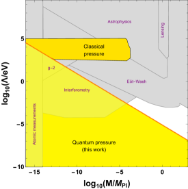
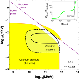
Figure 3: Bounds on chameleon-like models. Top: Exclusion regions on the standard chameleon with $n=1$, including bounds from Casimir experiments on the quantum and classical chameleon pressures. Bottom: Exclusion regions on the symmetron from Eöt-Wash on quantum and classical torques in presence of the intermediate sheet. Insert: Enhancement of the quantum force from an intermediate sheet as a function of its width.

A simple bound on the symmetron comes from molecular spectroscopy, in which case the Casimir-Polder force between nuclei is unscreened and results from Fichet (2018); Brax et al. (2018a) can be applied. For masses below the meV range (see Fig. 2 in Brax et al. (2018a)), the main bound on the symmetron comes from the Eöt-Wash experiment.

Interestingly the Eöt-Wash experiment is sensitive to the symmetron Casimir pressure because of the intermediate shield. The $L=55\,\mu$m measurement excludes a large part of the symmetron parameter space as shown in Fig. 3. A sensitivity up to $M\sim 1$ TeV and to $\mu\sim 58$ meV is obtained. In comparison, the classical exclusion region Upadhye (2013); Brax and Davis (2015) is finite, depends on $\lambda$ and vanishes for $\lambda\gtrsim 0.4$. The exclusion region near the transition requires a treatment of the VEV profile at the interface which is beyond the piecewise constant mass approximation used here.

Let us finally comment on the cosmological symmetron Hinterbichler and Khoury (2010); Hinterbichler et al. (2011). In such case the parameters of the symmetron model are typically chosen to satisfy $\mu^{2}M^{2}\sim H_{0}^{2}M_{\rm Pl}^{2}$, $\lambda\sim\frac{M_{\rm Pl}^{2}\mu^{2}}{M^{4}}$. Solar system tests require the coupling scale $M$ to be $M\lesssim 10^{-3}M_{\rm Pl}$. It turns out that the classical pressure Eq. (42) is overwhelmed by the quantum pressure at the scale of laboratory experiments. The main constraint comes thus from the Eot-Wash bound on the quantum pressure shown in Fig. 3. Since the lower bound on $M$ reaches only $\sim 1$ TeV, this leaves plenty of order of magnitudes in $M$ where the cosmological symmetron can exist. In terms of distance scales, the bound from the quantum pressure implies that the range of the symmetron force has to be larger than $\sim 3\cdot 10^{7}$ km. Similar conclusions apply to astrophysically relevant symmetrons, which tend to have larger masses $\mu$ and similar coupling scales $M$ O’Hare and Burrage (2018); Burrage et al. (2019).

VI Conclusion

We have studied the forces induced by chameleon-like particles in a fully-fledged quantum approach. Our formalism elucidates the role of screening in the quantum picture and naturally interpolates between the limits of Casimir and Casimir-Polder pressures. We have computed propagators with piecewise constant masses in an arbitrary number of 1D regions and analyzed in details the quantum chameleon pressure between plates. Our conclusions relative to the validity of the chameleon EFT differ from Upadhye et al. (2012) and are less restrictive. In the Eöt-Wash experiment we find that the sensitivity to the quantum pressure from chameleon-like fields is enhanced by the presence of the intermediate sheet. For both symmetron and standard chameleon models, the bounds on the quantum pressure exclude large and previously unconstrained regions of the parameter spaces.

Appendix A Variation of the vacuum energy

Here we detail the one-loop calculation of the vacuum energy and its variation with the source term $J$. We start with the partition function

$$Z[J]=\int{\cal D}\phi\,e^{i\int d^{4}x\left(\frac{1}{2}(\partial_{\mu}\phi)^{2}-V(\phi)-A(\phi)J\right)}\,.$$ (44)

Introducing $\phi=\phi_{\rm cl}+\eta$, where $\phi_{\rm cl}$ satisfies the classical equations of motion in the presence of the source $J$, gives

$$Z[J]=\int{\cal D}\eta\,e^{i\int d^{4}x\left(\frac{1}{2}(\partial_{\mu}(\phi_{\rm cl}+\eta))^{2}-V(\phi_{\rm cl}+\eta)-A(\phi_{\rm cl}+\eta)J\right)}.$$ (45)

An infinitesimal change in the source $J\rightarrow J+\delta J$ as the one induced by the variation in $L$ also changes the classical field $\phi_{\rm cl}\rightarrow\phi_{\rm cl}+\delta\phi_{\rm cl}$. The partition function, once the source has been shifted, is explicitly given by

$$Z[J+\delta J]=\int{\cal D}\eta\,$$ (46)

$$e^{-\int d^{4}x\left(\frac{1}{2}(\partial_{\mu}(\phi_{\rm cl}+\delta\phi_{\rm cl}+\eta))^{2}-V(\phi_{\rm cl}+\delta\phi_{\rm cl}+\eta)-A(\phi_{\rm cl}+\delta\phi_{\rm cl}+\eta)(J+\delta J)\right)}\,.$$

However the shift in $\phi_{\rm cl}$ can be absorbed in the integration variable using $\tilde{\eta}\equiv\eta+\delta\phi_{\rm cl}$, leaving

$$Z[J+\delta J]=$$ (47)

$$\int{\cal D}\tilde{\eta}\,e^{i\int d^{4}x\left(\frac{1}{2}(\partial_{\mu}(\phi_{\rm cl}+\tilde{\eta}))^{2}-V(\phi_{\rm cl}+\tilde{\eta})-A(\phi_{\rm cl}+\tilde{\eta})(J+\delta J)\right)}\,.$$

Notice that the source variation $\delta J$ now only appears in the last term of the action. Let us perform the functional derivative of $E[J]$ built from this variation. This gives us the quantum average of $\langle A\rangle_{J}$ as the variation only acts on the term in $A(\phi_{\rm cl}+\eta)(J+\delta J)$

$$\frac{E[J+\delta J]-E[J]}{\delta J}=\frac{i}{Z[J]}\frac{Z[J+\delta J]-Z[J]}{\delta J}=\langle A\rangle_{J}$$ (48)

in agreement with Eqs. (7), (8). Finally, on performs the $\eta$ integration of the $Z[J]$’s up to one-loop order, which is just the functional Gaussian integral

$$Z[J]\approx e^{i\int d^{4}x\left(\frac{1}{2}(\partial_{\mu}\phi_{\rm cl})^{2}-V(\phi_{\rm cl})-A(\phi_{\rm cl})J\right)}$$ (49)

$$\cdot\left({\rm det}\left[\partial+V^{\prime\prime}+A^{\prime\prime}J\right]\right)^{-1/2}\,,$$

$$Z[J+\delta J]\approx e^{i\int d^{4}x\left(\frac{1}{2}(\partial_{\mu}\phi_{\rm cl})^{2}-V(\phi_{\rm cl})-A(\phi_{\rm cl})(J+\delta J)\right)}$$ (50)

$$\cdot\left({\rm det}\left[\partial+V^{\prime\prime}+A^{\prime\prime}(J+\delta J)\right]\right)^{-1/2}\,.$$

The first line in Eqs. (49), (50) contains the classical action whose variation gives the classical force. The second line in these equations is the 1-loop functional determinant. Using these expressions in Eq. (48) gives the general formula Eq. (9) of Sec. II after some manipulations described in Eqs. (12)-(14).

Appendix B Green’s functions

B.1 Universal mass

In position-momentum space, the Feynman propagator takes the form

$$\Delta(z,z^{\prime})=\frac{e^{i\omega|z-z^{\prime}|}}{2\omega}\,$$ (51)

where one has introduced

$$\omega=\sqrt{(p_{0})^{2}-(p_{1})^{2}-(p_{2})^{2}+i\epsilon-m^{2}}\,.$$ (52)

This propagator can for instance be obtained by taking the Fourier transform of the usual 4-momentum space expression,

$$\int\frac{dp_{z}}{2\pi}\frac{i}{p^{2}-m^{2}+i\epsilon}e^{-ip_{z}(z-z^{\prime})}$$

$$=\int\frac{dp_{z}}{2\pi}\frac{-i}{p_{z}^{2}-\omega^{2}-i\epsilon}e^{-ip_{z}(z-z^{\prime})}$$

$$=\frac{-i}{2\pi}\begin{cases}(-2\pi i)\frac{e^{i\omega(z-z^{\prime})}}{-2\omega}\quad z>z^{\prime}\\ (2\pi i)\frac{e^{-i\omega(z-z^{\prime})}}{2\omega}\quad z<z^{\prime}\end{cases}$$

We can see that, as a result of the $i\epsilon$ prescription, the propagator vanishes at infinity. Note this is the boundary condition to impose if one calculates the position-momentum propagator directly from the equation of motion.

B.2 Piecewise constant mass

Position-momentum space is convenient to treat the case of a $z$-dependent mass $m(z)$. Here we give the key steps to calculate the general case of $N$ regions ${\cal D}_{i}$,

$$m^{2}(z)=\sum_{i=1}^{N}m^{2}_{i}\Theta(z\in{\cal D}_{i})\,,$$ (54)

with $\cup_{i=1}^{N}{\cal D}_{i}=\mathbf{R}$ and the interface between regions $j,j+1$ lies at the position $z_{j,j+1}$. The Green’s function satisfies

$$\partial_{z}^{2}\Delta(z,z^{\prime})-m^{2}(z)\Delta(z,z^{\prime})=i\delta(z-z^{\prime})\,.$$ (55)

The Feynman propagator is selected amongst the Green’s function by imposing that it vanishes at infinity. Defining $\omega(z)=\sqrt{(p_{0})^{2}-(p_{1})^{2}-(p_{2})^{2}+i\epsilon-m^{2}(z)}$, the solutions in each region are given by $\phi^{\pm}(z)=e^{\pm i\omega_{i}z}$. Requiring continuity of the solution and of its derivative, the solution over the full space reads

$$\phi=\begin{pmatrix}A^{+},A^{-}\end{pmatrix}\cdot\sum_{i=i}^{N}\left[{\cal C}_{i}\begin{pmatrix}\phi^{+}_{i}(x)\\ \phi^{-}_{i}(x)\end{pmatrix}\Theta(z\in{\cal D}_{i})\right]$$ (56)

with ${\cal C}_{i}=\prod_{j=i}^{i}{\cal T}_{j,j+1}\,$ where

$${\cal T}_{j,j+1}=\frac{1}{2\gamma_{j+1}}$$ (57)

$$\begin{pmatrix}(\gamma_{j}+\gamma_{j+1})e^{ix_{j,{j+1}}(\gamma_{j}-\gamma_{j+1})}&(\gamma_{j+1}-\gamma_{j})e^{ix_{j,{j+1}}(\gamma_{j}+\gamma_{j+1})}\\ (\gamma_{j+1}-\gamma_{j})e^{-ix_{j,{j+1}}(\gamma_{j}+\gamma_{j+1})}&(\gamma_{j}+\gamma_{j+1})e^{ix_{j,{j+1}}(\gamma_{j+1}-\gamma_{j})}\end{pmatrix}$$

is the transfer matrix given by the continuity conditions. The rest of the calculation of the Green’s function is given by standard ODE solving techniques, see for instance the appendix of Fichet for more details.

B.3 The two-regions case

In case of two regions, the Feynman propagator is found to be

$$\Delta(z,z^{\prime})=\begin{cases}\frac{e^{i\omega_{2}(z_{>}-z_{<})}}{2\omega_{2}}E_{2}(z_{<})\quad\quad z_{12}<z_{<}\\ \frac{e^{i(\omega_{2}(z_{>}-z_{12})-\omega_{1}(z_{<}-z_{12})}}{\omega_{1}+\omega_{2}}\quad z_{<}<z_{12}<z_{>}\\ \frac{e^{i\omega_{1}(z_{>}-z_{<})}}{2\omega_{1}}E_{1}(z_{>})\quad\quad z_{>}<z_{12}\end{cases}\,$$ (58)

where

$$E_{1}(z)=1+e^{i2(z_{12}-z)\omega_{1}}\frac{\omega_{1}-\omega_{2}}{\omega_{1}+\omega_{2}}$$

$$E_{2}(z)=1+e^{i2(z-z_{12})\omega_{2}}\frac{\omega_{2}-\omega_{1}}{\omega_{1}+\omega_{2}}\,$$

and where $x_{<}=\min(x,x^{\prime})$ and $x_{>}=\max(x,x^{\prime})$. The $E_{1}$, $E_{2}$ functions essentially describe how the presence of the boundary affects the propagator with both endpoints in the same region. When the boundary $x_{12}$ is rejected to infinity, one recovers the usual expression for fully homogeneous space.

Appendix C Vanishing at the boundary

Let us consider two regions of arbitrary shape ${\cal D}_{1}$, ${\cal D}_{2}$ where the mass takes values $m_{1}$, $m_{2}$. When $m_{2}\rightarrow\infty$ while other scales remain fixed, the homogeneous equation of motion in ${\cal D}_{2}$ corresponds to $m_{2}^{2}\Phi=0$ which is satisfied only if $\Phi=0$ at any point in ${\cal D}_{2}$. Moreover, since one requires continuity of the solution in the whole space, the value of $\Phi$ at the interface is also set to zero when $m_{2}\rightarrow\infty$. As a result, the problem is equivalent to having a field living in ${\cal D}_{1}$ and a Dirichlet boundary condition at the boundary of ${\cal D}_{2}$. This property can be directly seen in the planar case in, for instance, Eq. (58). For $\omega_{2}\rightarrow\infty$, it is clear that the propagator tends to zero inside ${\cal D}_{2}$ and at its boundary.

Appendix D Analytic structure

The quantum force at one loop has been calculated in Sec. III using a Wick rotation in $p_{0}$.

Let us first verify that the integrand $\Delta_{p}(L,L)$ (and $\Delta_{p}(z_{\infty},z_{\infty})$) are analytic in the first and third quadrant of the $p_{0}$ complex plane. The function $\Delta_{p}(L,L)$ depends on the $w_{i}^{\prime}s$ which have branch cuts on intervals along the real axis. The $i\epsilon$ prescription shifts the branch cuts just below the real axis for $p_{0}>0$ and just above the real axis for $p_{0}<0$. Thus the integrals in the $p_{0}$ plane along the real axis avoid the branch cuts, and no branch cut is crossed during the Wick rotation. Let us analyse the poles of the integrand. They would appear for

$$\frac{\omega_{1}-\omega_{2}}{\omega_{1}+\omega_{2}}\frac{\omega_{2}-\omega_{3}}{\omega_{2}+\omega_{3}}=e^{-2i\omega_{2}x_{0}}.$$ (60)

In the first quadrant of the $p_{0}$ complex plane and writing $\omega_{i}=|\omega_{i}|e^{i\theta_{i}}$ we have $\theta_{1,3}>\theta_{2}$ as $m_{1,3}>m_{2}$. These angles are all in the first quadrant too. This implies that

$$\left|\frac{\omega_{1}-\omega_{2}}{\omega_{1}+\omega_{2}}\frac{\omega_{2}-\omega_{3}}{\omega_{2}+\omega_{3}}\right|<1$$ (61)

whilst $|e^{-2i\omega_{2}x_{0}}|=1$. Hence the integrand has no poles in the first quadrant of the complex $p_{0}$ plane and one can perform a Wick’s rotation to the imaginary axis. A similar analysis applies to the third quadrant.

Finally, the $\Delta_{p}(L,L)-\Delta_{p}(z_{\infty},z_{\infty})$ integrand tends exponentially to zero at infinity on the arcs in the first and third quadrant, including on the real axis because of the $i\epsilon$ shift, hereby ensuing that the Wick rotation is valid just like in the familiar case of a universal mass.

Appendix E The Casimir-Polder force

In the main text, the Casimir-Polder force between plates (33) has been obtained as the unscreened limit of the general result Eq. (11), which is given by the path integral approach introduced in this work. Here we present an alternative calculation of the Casimir-Polder force between plates, done by first calculating the Casimir-Polder force between point-like sources using the Feynman diagram approach and then integrating over the plates. The result matches the unscreened limit (33) obtained in the main text.

Rewrite the source term as

$${\cal L}\supset A^{\prime\prime}J(x)=\frac{1}{2}m_{2}^{2}\eta^{2}+\frac{1}{2}\eta^{2}(\Theta(x<0)(m_{1}^{2}-m_{2}^{2})$$

$$+\Theta(r<x)(m_{3}^{2}-m_{2}^{2})).$$

We consider the presence of the plates as small perturbations, related to the coupling to individual nucleons via

$$(m_{i}^{2}-m_{2}^{2})=\frac{\rho_{i}}{\Lambda^{2}}=\frac{m_{N}n_{i}}{\Lambda^{2}}=\frac{m_{N}N_{i}}{V_{i}\Lambda^{2}}$$ (63)

where $\rho_{i}$ is the mass density, $n_{i}$ is the number density, $N_{i}$ is the total number of particles homogeneously distributed in the volume $V_{i}$.

We first compute the potential between two point sources (the single static nucleons), replacing $\rho$ by $m_{N}\delta^{(3)}(x)$. The corresponding source term is

$${\cal L}\supset AJ(x)=\frac{1}{2}\eta^{2}\left(\frac{m_{N}}{\Lambda^{2}}\delta^{(3)}(x^{i}-x^{i}_{a})+\frac{m_{N}}{\Lambda^{2}}\delta^{(3)}(x^{i}-x^{i}_{b})\right)\,.$$ (64)

The bubble diagram is

$$i{\cal M}=-\frac{m_{N}^{2}}{\Lambda^{4}}\,4m_{N}^{2}\,\frac{1}{2}\int\frac{dk^{3}}{(2\pi)^{3}}\frac{e^{i\omega_{2}|z_{1}-z_{2}|)}}{2\omega_{2}}\frac{e^{i\omega^{\prime}_{2}|z_{1}-z_{2}|)}}{2\omega^{\prime}_{2}}$$ (65)

where $\omega_{2}=\sqrt{k^{2}-m_{2}^{2}}$, $\omega^{\prime}_{2}=\sqrt{(k+p)^{2}-m_{2}^{2}}$. We have used the explicit expression for the Feynman propagator. In this formalism $k,p$ are 3-momenta, $k=(k^{0},k^{1},k^{2})$ for example. The scattering potential is given by

$$\tilde{V}(p,z_{1}-z_{2})=-\frac{\cal{M}}{4m_{N}^{2}}$$

$$=-i\frac{m_{N}^{2}}{\Lambda^{4}}\frac{1}{2}\int\frac{dk^{3}}{(2\pi)^{3}}\frac{e^{i\gamma_{2}|z_{1}-z_{2}|)}}{2\omega_{2}}\frac{e^{i\omega_{2}^{\prime}|z_{1}-z_{2}|)}}{2\omega_{2}^{\prime}}\,.$$

The sources are static hence $p_{0}$ can readily be set to zero. The spatial potential is given by the Fourier transform of this,

$$V\left(\sqrt{(z_{1}-z_{2})^{2}+x_{\parallel}^{2}}\right)=\int\frac{d^{2}p_{\parallel}}{(2\pi)^{2}}\tilde{V}(p_{\parallel},z_{1},z_{2})e^{ip_{\parallel}\cdot x_{\parallel}}$$ (67)

where $x_{\parallel}=(x^{1},x^{2})$. We are also going to average the potential over plates with separation $L$,

$$V_{\rm plates}=N_{1}V_{1}^{-1}N_{3}V_{3}^{-1}\times$$

$$\int d^{2}x_{\parallel}\int_{-\infty}^{0}dz_{1}\int d^{2}x^{\prime}_{\parallel}\int^{\infty}_{L}dz_{2}\int\frac{d^{2}p_{\parallel}}{(2\pi)^{2}}\tilde{V}(p_{\parallel},z_{1},z_{2})e^{ip_{\parallel}\cdot x_{\parallel}}$$

where $V_{1}$, $V_{3}$ are the volumes of regions 1 and 3. One has $\int d^{2}x^{\prime}_{\parallel}=S$. We can see that the integrals simplify since

$$\int d^{2}x_{\parallel}\frac{d^{2}p_{\parallel}}{(2\pi)^{2}}e^{ip_{\parallel}\cdot x_{\parallel}}F(p_{\parallel})=F(0)\,.$$ (69)

Thus the potential is simply

$$V_{\rm plates} =Sn_{1}n_{3}\int_{-\infty}^{0}dz_{1}\int^{\infty}_{L}dz_{2}\tilde{V}(0,z_{1},z_{2})$$ (70)

$$=-iSn_{1}n_{3}\frac{m_{N}^{2}}{\Lambda^{4}}\frac{1}{2}\int\frac{dk^{3}}{(2\pi)^{3}}\int_{-\infty}^{0}dz_{1}\int^{\infty}_{L}dz_{2}\frac{e^{i2\omega_{2}(z_{2}-z_{1})}}{4\omega^{2}_{2}}$$ (71)

$$=Sn_{1}n_{3}\frac{m_{N}^{2}}{\Lambda^{4}}\,\int\frac{dk_{E}^{3}}{(2\pi)^{3}}\int_{-\infty}^{0}dz_{1}\int^{\infty}_{L}dz_{2}\frac{e^{-2\gamma_{2}(z_{2}-z_{1})}}{-8(\gamma_{2})^{2}}$$ (72)

$$=-Sn_{1}n_{3}\frac{m_{N}^{2}}{\Lambda^{4}}\,\int\frac{dk_{E}^{3}}{(2\pi)^{3}}\frac{e^{-2\gamma_{2}L}}{32(\gamma_{2})^{4}}$$ (73)

$$=-S(m_{1}^{2}-m_{2}^{2})(m_{3}^{2}-m_{2}^{2})\frac{m_{N}^{2}}{\Lambda^{4}}\,\int\frac{dk_{E}^{3}}{(2\pi)^{3}}\frac{e^{-2\gamma_{2}L}}{32(\gamma_{2})^{4}}\,.$$ (74)

In the last line one has used $\frac{n_{i}\,m_{N}}{\Lambda^{2}}=m_{i}^{2}-m_{2}^{2}$. Finally the pressure is obtained by taking the derivative

$$P=S^{-1}\partial_{L}V_{\rm plates}=(m_{1}^{2}-m_{2}^{2})(m_{3}^{2}-m_{2}^{2})\,\int\frac{dk_{E}^{3}}{(2\pi)^{3}}\frac{e^{-2\gamma_{2}L}}{16(\gamma_{2})^{3}}\,.$$ (75)

This reproduces (33 ) in the main text.

References

References

- Brax (2013) P. Brax, Class. Quant. Grav. 30, 214005 (2013).
- Bertotti et al. (2003) B. Bertotti, L. Iess, and P. Tortora, Nature 425, 374 (2003).
- Williams et al. (2012) J. G. Williams, S. G. Turyshev, and D. Boggs, Class. Quant. Grav. 29, 184004 (2012), arXiv:1203.2150 [gr-qc] .
- Khoury and Weltman (2004a) J. Khoury and A. Weltman, Phys.Rev.Lett. 93, 171104 (2004a), arXiv:astro-ph/0309300 [astro-ph] .
- Khoury and Weltman (2004b) J. Khoury and A. Weltman, Phys. Rev. D69, 044026 (2004b), arXiv:astro-ph/0309411 .
- Brax et al. (2004a) P. Brax, C. van de Bruck, A.-C. Davis, J. Khoury, and A. Weltman, Phys. Rev. D70, 123518 (2004a), arXiv:astro-ph/0408415 .
- Brax et al. (2010a) P. Brax, C. van de Bruck, D. F. Mota, N. J. Nunes, and H. A. Winther, Phys. Rev. D82, 083503 (2010a), arXiv:1006.2796 [astro-ph.CO] .
- Pietroni (2005) M. Pietroni, Phys.Rev. D72, 043535 (2005), arXiv:astro-ph/0505615 [astro-ph] .
- Olive and Pospelov (2008) K. A. Olive and M. Pospelov, Phys. Rev. D77, 043524 (2008), arXiv:0709.3825 [hep-ph] .
- Hinterbichler and Khoury (2010) K. Hinterbichler and J. Khoury, Phys. Rev. Lett. 104, 231301 (2010), arXiv:1001.4525 [hep-th] .
- Brax and Pignol (2011) P. Brax and G. Pignol, Phys. Rev. Lett. 107, 111301 (2011), arXiv:1105.3420 [hep-ph] .
- Jenke et al. (2014) T. Jenke et al., Phys. Rev. Lett. 112, 151105 (2014), arXiv:1404.4099 [gr-qc] .
- Lemmel et al. (2015) H. Lemmel, P. Brax, A. N. Ivanov, T. Jenke, G. Pignol, M. Pitschmann, T. Potocar, M. Wellenzohn, M. Zawisky, and H. Abele, Phys. Lett. B743, 310 (2015), arXiv:1502.06023 [hep-ph] .
- Cronenberg et al. (2018) G. Cronenberg, P. Brax, H. Filter, P. Geltenbort, T. Jenke, G. Pignol, M. Pitschmann, M. Thalhammer, and H. Abele, Nature Phys. 14, 1022 (2018).
- Burrage and Copeland (2016) C. Burrage and E. J. Copeland, Contemp. Phys. 57, 164 (2016), arXiv:1507.07493 [astro-ph.CO] .
- Jaffe et al. (2017) M. Jaffe, P. Haslinger, V. Xu, P. Hamilton, A. Upadhye, B. Elder, J. Khoury, and H. Müller, Nature Phys. 13, 938 (2017), arXiv:1612.05171 [physics.atom-ph] .
- Brax et al. (2007) P. Brax, C. van de Bruck, A.-C. Davis, D. F. Mota, and D. J. Shaw, Phys. Rev. D76, 124034 (2007), arXiv:0709.2075 [hep-ph] .
- Brax et al. (2010b) P. Brax, C. van de Bruck, A. C. Davis, D. J. Shaw, and D. Iannuzzi, Phys. Rev. Lett. 104, 241101 (2010b), arXiv:1003.1605 [quant-ph] .
- Almasi et al. (2015) A. Almasi, P. Brax, D. Iannuzzi, and R. I. P. Sedmik, Phys. Rev. D91, 102002 (2015), arXiv:1505.01763 [physics.ins-det] .
- Adelberger et al. (2007) E. G. Adelberger, B. R. Heckel, S. A. Hoedl, C. D. Hoyle, D. J. Kapner, and A. Upadhye, Phys. Rev. Lett. 98, 131104 (2007), arXiv:hep-ph/0611223 [hep-ph] .
- Damour and Esposito-Farese (1992) T. Damour and G. Esposito-Farese, Class. Quant. Grav. 9, 2093 (1992).
- Note (1) Our conventions follow the ones of Peskin and Schroeder (1995).
- Peskin and Schroeder (1995) M. E. Peskin and D. V. Schroeder, An introduction to quantum field theory (Westview, Boulder, CO, 1995).
- Brax and Davis (2015) P. Brax and A.-C. Davis, Phys. Rev. D91, 063503 (2015), arXiv:1412.2080 [hep-ph] .
- Weinberg (1989) S. Weinberg, Rev. Mod. Phys. 61, 1 (1989), [,569(1988)].
- Milton (2003) K. A. Milton, Phys. Rev. D68, 065020 (2003), arXiv:hep-th/0210081 [hep-th] .
- Fichet (2018) S. Fichet, Phys. Rev. Lett. 120, 131801 (2018), arXiv:1705.10331 [hep-ph] .
- Brax et al. (2018a) P. Brax, S. Fichet, and G. Pignol, Phys. Rev. D97, 115034 (2018a), arXiv:1710.00850 [hep-ph] .
- Note (2) The two-loop contribution also renormalizes the leading order coupling. For instance in the case of plates studied in Sec. III, the two loop contribution is . The main divergence cancels and the remaining divergence is absorbed in the renormalization of the leading coupling, leaving only the finite term .
- Brax et al. (2004b) P. Brax, C. van de Bruck, and A. C. Davis, JCAP 0411, 004 (2004b), arXiv:astro-ph/0408464 [astro-ph] .
- Carena et al. (2002) M. Carena, T. M. P. Tait, and C. E. M. Wagner, Acta Phys. Polon. B33, 2355 (2002), arXiv:hep-ph/0207056 [hep-ph] .
- Carena et al. (2003) M. Carena, E. Ponton, T. M. P. Tait, and C. E. M. Wagner, Phys. Rev. D67, 096006 (2003), arXiv:hep-ph/0212307 [hep-ph] .
- Upadhye et al. (2012) A. Upadhye, W. Hu, and J. Khoury, Phys. Rev. Lett. 109, 041301 (2012), arXiv:1204.3906 [hep-ph] .
- Brax and Pitschmann (2018) P. Brax and M. Pitschmann, Phys. Rev. D97, 064015 (2018), arXiv:1712.09852 [gr-qc] .
- Brax et al. (2008) P. Brax, C. van de Bruck, A.-C. Davis, and D. J. Shaw, Phys. Rev. D78, 104021 (2008), arXiv:0806.3415 [astro-ph] .
- Upadhye (2012) A. Upadhye, Phys. Rev. D86, 102003 (2012), arXiv:1209.0211 [hep-ph] .
- Kapner et al. (2007) D. J. Kapner, T. S. Cook, E. G. Adelberger, J. H. Gundlach, B. R. Heckel, C. D. Hoyle, and H. E. Swanson, Phys. Rev. Lett. 98, 021101 (2007), arXiv:hep-ph/0611184 [hep-ph] .
- Burrage and Sakstein (2016) C. Burrage and J. Sakstein, JCAP 1611, 045 (2016), arXiv:1609.01192 [astro-ph.CO] .
- Brax et al. (2018b) P. Brax, A.-C. Davis, B. Elder, and L. K. Wong, Phys. Rev. D97, 084050 (2018b), arXiv:1802.05545 [hep-ph] .
- Bordag (2009) M. Bordag, Advances in the Casimir Effect, International Series of Monogr (OUP Oxford, 2009).
- Decca et al. (2007a) R. S. Decca, D. Lopez, E. Fischbach, G. L. Klimchitskaya, D. E. Krause, and V. M. Mostepanenko, Eur. Phys. J. C51, 963 (2007a), arXiv:0706.3283 [hep-ph] .
- Decca et al. (2007b) R. S. Decca, D. Lopez, E. Fischbach, G. L. Klimchitskaya, D. E. Krause, and V. M. Mostepanenko, Phys. Rev. D75, 077101 (2007b), arXiv:hep-ph/0703290 [hep-ph] .
- Upadhye (2013) A. Upadhye, Phys. Rev. Lett. 110, 031301 (2013), arXiv:1210.7804 [hep-ph] .
- Hinterbichler et al. (2011) K. Hinterbichler, J. Khoury, A. Levy, and A. Matas, Phys. Rev. D84, 103521 (2011), arXiv:1107.2112 [astro-ph.CO] .
- O’Hare and Burrage (2018) C. A. O’Hare and C. Burrage, Phys. Rev. D98, 064019 (2018), arXiv:1805.05226 [astro-ph.CO] .
- Burrage et al. (2019) C. Burrage, E. J. Copeland, C. Käding, and P. Millington, Phys. Rev. D99, 043539 (2019), arXiv:1811.12301 [astro-ph.CO] .
- (47) S. Fichet, To appear.