High Performance Zero-Memory Overhead Direct Convolutions

Abstract

The computation of convolution layers in deep neural networks typically rely on high performance routines that trade space for time by using additional memory (either for packing purposes or required as part of the algorithm) to improve performance. The problems with such an approach are two-fold. First, these routines incur additional memory overhead which reduces the overall size of the network that can fit on embedded devices with limited memory capacity. Second, these high performance routines were not optimized for performing convolution, which means that the performance obtained is usually less than conventionally expected. In this paper, we demonstrate that direct convolution, when implemented correctly, eliminates all memory overhead, and yields performance that is between 10% to 400% times better than existing high performance implementations of convolution layers on conventional and embedded CPU architectures. We also show that a high performance direct convolution exhibits better scaling performance, i.e. suffers less performance drop, when increasing the number of threads.

1 Introduction

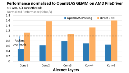
Figure 1: High performance direct convolution implementation achieves higher performance than a high performance matrix multiplication routine, whereas matrix-multiplication based convolution implementations suffers from packing overheads and is limited by the performance of the matrix multiplication routine

Conventional wisdom suggests that computing convolution layers found in deep neural nets via direct convolution is not efficient. As such, many existing methods for computing convolution layers (Jia et al., 2014; Cho & Brand, 2017) in deep neural networks are based on highly optimized routines (e.g. matrix-matrix multiplication) found in computational libraries such as the Basic Linear Algebra Subprograms (BLAS) (Dongarra et al., 1990). In order to utilize the matrix-matrix multiplication routine, these frameworks reshape and selectively duplicate parts of the original input data (collectively known as packing); thereby incurring additional memory space for performance.

There are two problems with this approach: First, the additional work of reshaping and duplicating elements of the input data is a bandwidth-bounded operation that incurs an additional, and non-trivial time penalty on the overall system performance. Second, and more importantly, matrices arising from convolution layers often have dimensions that are dissimilar from matrices arising from traditional high performance computing (HPC) application. As such, the matrix-matrix multiplication routine typically does not achieve as good a performance on convolution matrices as compared to HPC matrices.

To illustrate these drawbacks of existing methods, consider the 4-thread performance attained on various convolution layers in AlexNet using an AMD Piledriver architecture shown in Figure 1. In this plot, we present performance of 1) a traditional matrix-multiply based convolution implementation linked to OpenBLAS (OpenBLAS, ) (blue) and 2) our proposed high performance direct convolution implementation (yellow). Performance of both implementations are normalized to the performance of only the matrix-matrix multiplication routine (dashed line). This dashed line is the performance attained by matrix-matrix multiplication if packing is free. Notice that the performance of OpenBLAS + Packing achieves less than 80% of the performance of matrix multiplication itself. This implies that the packing routine degrades the overall performance by more than 20%. In contrast, our custom direct convolution implementation yields performance that exceeds the expert-implemented matrix-matrix multiplication routine, even if packing was free. In addition, we attained the performance without any additional memory overhead.

It is timely to revisit how convolution layers are computed as machine learning tasks based on deep neural networks are increasingly being placed on edge devices (Schuster, 2010; Lee & Verma, 2013). These devices are often limited in terms of compute capability and memory capacity (Gokhale et al., 2014; Dundar et al., ). This means that existing methods that trade memory capacity for performance are no longer viable solutions for these devices. Improving performance and reducing memory overheads also bring about better energy efficiency (Zhang et al., 2014). While many work have focused on reducing the memory footprint of the convolution layer through the approximation (Kim et al., 2015), quantilization(Gong et al., 2014), or sparsification of the weights (Han et al., 2016), few work tackle the additional memory requirements required in order to use high performance routines.

Contributions. Herein lies the contributions of this paper:

• High performance direct convolution. We show that a high performance implementation of direct convolution can out-perform a expert-implemented matrix-matrix multiplication based convolution in terms of amount of actual performance, parallelism, and reduced memory overhead. This demonstrates that that direct convolution is a viable means of computing convolution layers.

• Data layouts for input/output feature maps and kernel weights. We proposed new data layouts for storing the input, output and kernel weights required for computing a convolution layer using our direct convolution algorithm. The space required for these new data layouts is identical to the existing data storage scheme for storing the input, output and kernel weights prior to any packing or duplication of elements.

2 Inefficiency of Non-direct Convolutions

In this section, we highlight the inefficiency of computing convolution with existing methods used in many deep learning frameworks.

2.1 Fast Fourier Transform-based Implementations

Fast Fourier Transform (FFT)-based implementations (Vasilache et al., 2014; Mathieu et al., 2013) of convolution were proposed as a means of reducing the number of floating point operations that are performed when computing convolution in the frequency domain. However, in order for the computation to proceed, the kernel weights have to be padded to the size of the input image, incurring significantly more memory than necessary, specially when the kernels themselves are small (e.g. $3\times 3$).

Alternative approaches have been proposed to subdivide the image into smaller blocks or tiles (Dukhan, ). However, such approaches also require additional padding of the kernel weights to a convenient size (usually a power of two) in order to attain performance. Even padding the kernel weights to small multiples of the architecture register size (e.g. 8 or 16) will result in factors of 7 to 28 increase in memory requirement. This additional padding and transforming the kernel to the frequency domain can be minimized by performing the FFT on-the-fly as part of the computation of the convolution layer. This, however, incurs significant performance overhead, especially on embedded devices, as we will show in the performance section (Section 5).

2.2 Matrix Multiplication-based Implementations

Another common approach is to cast the inputs (both the image and kernel weights) into matrices and leverage the high performance matrix-matrix multiplication routine found in the Level 3 Basic Linear Algebra Subprogram (BLAS) (Dongarra et al., 1990) for computation. There are two major inefficiencies with this approach:

• Additional memory requirements. In order to cast the image into a matrix, a lowering operation is performed to cast the three dimensional image into a two dimensional matrix. Typically, this is performed via an operation conventionally called im2col that copies the $W_{i}\times H_{i}\times C_{i}$ image into a $(H_{f}\times W_{f}\times C_{i})\times(H_{o}\times W_{o})$ matrix which is then used as an input to the matrix-matrix multiplication call. During this lowering process, appropriate elements are also duplicated. The additional memory required grows quadratically with the problem size (Cho & Brand, 2017).

  Cho and Brand (Cho & Brand, 2017) proposed an alternative lowering mechanism that is more memory efficient by reducing the amount of duplication required during the packing process. In their lowering routine, the memory footprint is reduced by an average factor of 3.2 times over im2col. This is achieved by eliminating the amount of duplication required at the expense of additional matrix-matrix multiplication calls. Nonetheless, this is still an additional memory requirement, and their computation still relies on a matrix-matrix multiplication that is often sub-optimal for matrices arising from convolution.

• Sub-optimal matrix matrix multiplication. In most BLAS libraries (e.g. GotoBLAS (Goto & van de Geijn, 2008), OpenBLAS (OpenBLAS, ), BLIS (Van Zee & van de Geijn, 2015)), the matrix-matrix multiplication routine achieves the best performance when the inner dimensions, i.e. the dimension that is common between the two input matrices, of the input matrices are small compared to the overall dimensions of the output matrix. This particular set of matrix shapes is commonly found in scientific and engineering codes, for which these libraries are optimized. However, this particular set of shapes exercise only one out of six possible algorithms for matrix-matrix multiplication (Goto & van de Geijn, 2008).

  Recall that the im2col reshapes the input into a $(H_{f}\times W_{f}\times C_{i})\times(H_{o}\times W_{o})$ matrix. This means that the inner dimensions of the input matrices are often the larger of two dimensions (See Figure 2). As such, the performance of matrix matrix multiplication on this particular set of input shapes is often significantly below the best achievable performance. It has been shown that alternative algorithms for computing matrix multiplications should be pursued for shapes similar to that arising from convolution layers (Gunnels et al., 2001).

  Another reason that matrix-matrix multiplication is inefficient for convolution layers is that parallelism in existing BLAS libraries are obtained by partitioning the rows and columns of the input matrices (Smith et al., 2014). This partitioning of the matrices skews the matrix shapes even farther away from the shapes expected by the matrix-matrix multiplication routine. As such, the efficiency of the routine suffers as the number of threads increases.

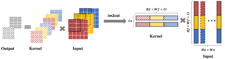
Figure 2: The $5\times 5$ input image with 3 different channels (denoted with different colors) is convolved with two separate kernels to obtain a $3\times 3$ output with two output channels. Packing is performed to turn three dimensional input images (left) into a two dimensional matrix (right) in order to utilize a high performance matrix multiplication routine. As $C_{o}$ and/or $(H_{o}\times W_{o})$ are often less than $H_{f}\times W_{f}\times C_{i}$, performance of standard matrix-matrix multiplication in many BLAS libraries are often sub-optimal.

3 High Performance Direct Convolution

Algorithm 1 Naive Convolution Algorithm

  Input: Input $\mathcal{I}$, Kernel Weights $\mathcal{F}$, stride $s$;

  Output: Output $\mathcal{O}$

  for $i=1$ to $C_{i}$ do

     for $j=1$ to $C_{o}$ do

        for $k=1$ to $W_{o}$ do

           for $\ell=1$ to $H_{o}$ do

              for $m=1$ to $W_{f}$ do

                 for $n=1$ to $H_{f}$ do

                    $\mathcal{O}_{j,k,\ell}+=\mathcal{I}_{i,k\times s+m,\ell\times s+n}\times\mathcal{F}_{i,j,m,n}$

A naive implementation of direct convolution (See Algorithm 1) is essentially six perfectly-nested loops around a multiply-and-accumulate computational statement that computes a single output element. Any permutation of the ordering of the loops will yield the correct result. However, in order to obtain a high performance implementation of direct convolution, it is essential that these loops and their order are appropriately mapped to the given architecture.

3.1 Strategy for mapping loops to architecture

Our strategy for mapping the loops to a model architecture is similar to the analytical model for high performance matrix-matrix multiplication (Low et al., 2016). (1) We first introduce the model architecture used by high performance matrix-matrix multiplication. (2) Next, we identify loops that utilize the available computational units efficiently. (3) Finally, we identify the order of the outer loops in order to improve data reuse, which in turn will reduce the amount of performance-degrading stalls introduced into the computation. In this discussion, we use the index variables show in Algorithm 1 ($i,j,k,\ell,m,n$) to differentiate between the loops.

3.1.1 Model architecture

We use the model architecture used the analytical model for high performance matrix-multiplication (Low et al., 2016). The model architecture is assumed to have the following features:

• Vector registers. We assume that our model architecture uses single instruction multiple data (SIMD) instruction sets. This means that each operation simultaneously performs its operation on $N_{\mbox{vec}}$ scalar output elements. We also make the assumption that $N_{\mbox{vec}}$ is a power of two. When $N_{\mbox{vec}}$ is one, this implies that only scalar computations are available. In addition, a total of $N_{\mbox{reg}}$ logical registers are addressable.

• FMA instructions. We assume the presence of $N_{\mbox{fma}}$ units that can compute fused multiply-add instructions (FMA). Each FMA instruction computes a multiplication and an addition. Each of these $N_{\mbox{fma}}$ units can compute one FMA instruction every cycle (i.e., the units can be fully pipelined), but each FMA instruction has a latency of $L_{\mbox{fma}}$ cycles. This means that $L_{\mbox{fma}}$ cycles must pass since the issuance of the FMA instruction before a subsequent dependent FMA instruction can be issued.

• Load/Store architecture. We assume that the architecture is a load/store architecture where data has to be loaded into registers before operations can be performed on the loaded data. On architectures with instructions that compute directly from memory, we assume that those instructions are not used.

3.1.2 Loops to saturate computations

The maximum performance on our model architecture is attained when all $N_{\mbox{fma}}$ units are computing one FMA per cycle. However, because each FMA instruction has a latency of $L_{\mbox{fma}}$ cycles, this means that there must at least be $L_{\mbox{fma}}$ independent FMA instructions issued to each computational unit. As each FMA instruction can compute $N_{\mbox{vec}}$ output elements, this means that

$$\mathcal{E}\geq N_{\mbox{vec}}N_{\mbox{fma}}L_{\mbox{fma}},$$ (1)

where $\mathcal{E}$ is the minimum number of independent output elements that has to be computed in each cycle in order to reach the maximum attainable performance.

Having determine that at least $\mathcal{E}$ output elements must be computed in each cycle, the next step is to determine the arrangement of these output elements within the overall output of the convolution layer. Notice that the output has three dimensions ($H_{o}\times W_{o}\times C_{o}$) where $H_{o}$ and $W_{o}$ are primarily a function of the input sizes, while $C_{o}$ is a design parameter of the convolution layer. Since $\mathcal{E}$ must be a multiple of $N_{vec}$, i.e. a power-of-two, and $C_{o}$ can be chosen (and is the case in practice) to be a power-of-two, the $j$ loop is chosen as the inner-most loop.

As the minimum number $\mathcal{E}$ is highly dependent on the number and capability of the FMA computation units, we want to ensure that there are sufficient output elements to completely saturate computation. As such, the $k$ loop that iterates over the elements in the same row of the output image is chosen to be the loop around the $j$ loop .

3.1.3 Loops to optimize data reuse

The subsequent loops are ordered to bring data to the computational units as efficiently as possible.

Recall that the inner two loops ($j$ and $k$) iterate over multiple output elements to ensure that sufficient independent FMA operations can be performed to avoid stalls in the computation units. As our model architecture is a load/store architecture, this means that these output elements are already in registers. Therefore, we want to bring in data that allows us to accumulate into these output elements.

Recall that to compute a single output element, all $H_{f}\times W_{f}\times C_{i}$ weights are multiplied with the appropriate element from the input image and accumulated into the output element. This naturally means that the next three loops in sequence from the inner-most to outer-most are the $i,m,n$ loops. This order of the loops is determined based on the observation that the input of most convolution layers is the output of another convolution layer. This means that it would be advisable if data from both the input and output are accessed in the same order. As such, we want to access the input elements in the channels ($i$) before rows ($n$), which gives us the $i,n,m$ ordering of the loops.

Having decided on five of the original six loops, this means that outermost loop has to be the $l$ loop. This loop traverses over the remaining through different rows of the output. The original loop order as shown in Algorithm 1 ($i,j,k,l,m,n$) is transformed to the ($l,n,m,i,k,j$) loop ordering as shown in Algorithm 2.

Algorithm 2 Reorder Convolution Algorithm

  Input: Input $\mathcal{I}$, Kernel Weights $\mathcal{F}$, stride $s$;

  Output: Output $\mathcal{O}$

  for $\ell=1$ to $H_{o}$ do

     for $n=1$ to $H_{f}$ do

        for $m=1$ to $W_{f}$ do

           for $i=1$ to $C_{i}$ do

              for $k=1$ to $W_{o}$ do

                 for $j=1$ to $C_{o}$ do

                    $\mathcal{O}_{j,k,\ell}+=\mathcal{I}_{i,k\times s+m,\ell\times s+n}\times\mathcal{F}_{i,j,m,n}$

3.1.4 Blocking for the memory hierarchy

Register Blocking.The astute reader will recognize that we have conveniently ignored the fact that $\mathcal{E}$, the number of minimum output elements required to sustain peak performance,is upper bounded by the number of registers as described by the following inequality:

$$\mathcal{E}\leq N_{\mbox{reg}}{N_{\mbox{vec}}}.$$ (2)

This upper bound imposed by the number of available registers means that at most $N_{\mbox{reg}}N_{\mbox{vec}}$ elements can be kept in the registers. This means that instead of iterating over all $C_{o}\times W_{o}$ elements, loop blocking/tiling (Wolfe, 1989) with block sizes of $C_{o,b}$ and $W_{o,b}$ has to be applied to the two inner-most loops to avoid register-spilling that will degrade performance.

Applying loop blocking to the original $j$ and $k$ loops decomposes a row from each of the output channel into smaller output images, each of which having a row width and output channel of $W_{o,b}$, and $C_{o,b}$ respectively. Since loop blocking decomposes the overall convolution into smaller convolutions, the loop ordering previously described remains applicable. However, we now need to determine how to traverse over the smaller convolutions.

The loops $j^{\prime}$ and $k^{\prime}$ iterate over the blocks in the channel and row dimensions of the output, respectively. In addition, loops $jj$ and $kk$ iterate with the respective blocks of channels and rows. We make the observation accessing input elements in the same row will require us to also access kernel weights in the same row. This suggest that the ordering of the loop should be similar to the loops traversing across the kernel weights. As such, the $k^{\prime}$ loop is nested between $\ell$ and $n$ loops. The $j^{\prime}$ loop is set to be the outermost loop since it is a parallel loop that facilitates parallelization.

Cache Blocking. On architecture with more levels in the memory hierarchy, i.e. architectures with caches, we can further partition the input dataset into smaller partitions such that they fit into the appropriate levels of the cache. Recall that the loops around $jj$ and $kk$ accumulates $H_{f}\times W_{f}\times C_{i}$ intermediate results into the output stored in the register. Since $H_{f}$ and $W_{f}$, i.e. the size of the kernel weights, are typically smaller than $C_{i}$, we choose to partition the $i$ loop which iterates over $C_{i}$ input channels for the next level in the memory hierarchy.

The final algorithm for high performance direct convolution is shown in Algorithm 3.

Algorithm 3 Parallelized Direct Convolution Algorithm

  Input: Input $\mathcal{I}$, Kernel Weights $\mathcal{F}$, stride $s$;

  Output: Output $\mathcal{O}$

  for $j^{\prime}=1$ to $C_{o}/C_{o,b}$ in Parallel do

     for $i^{\prime}=1$ to $C_{i}/C_{i,b}$  do

        for $\ell=1$ to $H_{o}$  do

           for $k^{\prime}=1$ to $W_{o}/W_{o,b}$ do

              for $n=1$ to $H_{f}$ do

                 for $m=1$ to $W_{f}$ do

                    for $ii=1$ to $C_{i,b}$ do

                       for $kk=1$ to $W_{o,b}$ do

                          for $jj=1$ to $C_{o,b}$ do

                              $\begin{array}[]{l}\mathcal{O}_{j^{\prime}C_{o,b}+jj,{k^{\prime}W_{o,b}}+kk,\ell}\quad+=\\ \quad\mathcal{I}_{{i^{\prime}C_{i,b}}+ii,{sk^{\prime}W_{o,b}}+kk+m,\ell s+n}~{}\times\\ \quad\mathcal{F}_{{i^{\prime}C_{i,b}}+ii,j^{\prime}\times C_{o,b}+jj,m,n}\end{array}$

3.2 Parallelism

In order to identify possible parallel algorithms, we first make the observation that all output elements can be computed in parallel. Since the output is a three dimensional object ($H_{o}\times W_{o}\times C_{o}$), this means that parallelism can be extracted in at least three different dimensions.

Our direct convolution implementation extracts parallelism in the output channel ($C_{o}$) dimension. Each thread is assigned a block of output elements to compute, where each block of output elements is of size $H_{o}\times W_{o}\times C_{o}/p$, where $p$ is the number of threads used.

4 Convolution-Friendly Data Layout

We proposed new data layouts for the input and kernel data so that data is accessed in unit stride as much as possible. This improves data access and avoids costly stalls when accessing data from lower levels of the memory hierarchy. A key criteria in revising the layout is that the output and the input image should have the same data layout. This is because the input of most convolution layers is the output of another convolution layer. Keeping them in the same data layout will avoid costly data reshape between convolution layers. However, to ensure compatibility with original input images, we do not impose the proposed layout on the inputs to the first convolution layer.

4.1 Input/Output Layout

We want to access the output data in unit stride. Therefore, we determine the output data layout by considering how the elements are accessed using the loop ordering shown in Algorithm 3. Data accessed in the inner loops should be arranged closer together in memory than data accessed in the outer loops.

Five loops ($j,k,\ell,kk,jj$) iterate over the output data, which suggests a five-dimensional data layout. However, this is sub-optimal if we were to use it for the input data. This is because $W_{f}$ elements in an input row is required to compute one output element. With the five-dimensional layout, a row of the input is blocked into blocks of $W_{o,b}$ elements. This means that output elements that require input elements from two separate $W_{o,b}$ blocks will incur a large penalty as these input elements are separated over a large distance in memory. As such we do not layout the data according to the $kk$ loop.

The proposed input/output layout is shown in Figure 3 (left). The output data is organized into sequential blocks of $H_{o}\times W_{o}\times C_{o,b}$, where in each block, elements are first laid out in the channel dimension, before being organized into a $H_{o}\times W_{o}$ row-major-order matrix of pencils of length $C_{o,b}$.

4.2 Kernel Layout

Similar to the input/output layout, we use the loop ordering to determine how to order the kernel weights into sequential memory. Notice that the $\ell,k^{\prime},kk$ loops in Algorithm 3 iterates over the height and width of the output in a single output channel. As all output elements in the same output channel share the same kernel weights, these loops provide no information as to how the kernel weights should be stored. As such, we only consider the remaining six loops.

The kernel layout proposed by the remaining six loops is shown in Figure 3 (right). The fastest dimension in the kernel layout is the blocked output channel ($C_{o,b}$) dimension, and is dictated by the inner-most loop. The remaining dimensions from fastest to slowest are the blocked input channel ($C_{i,b}$), followed by the columns ($W_{f}$) and rows ($H_{f}$) of the kernel, the input channels ($C_{i}/C_{i,b}$) and finally the output channels ($C_{o}/C_{o,b}$).

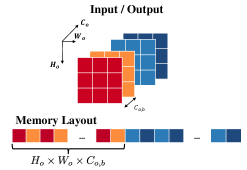
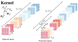
Figure 3: Convolution-friendly layout for input/output (left) and kernel weights (right). The output data is organized into sequential blocks of $H_{o}\times W_{o}\times C_{o,b}$, where in each block, the fastest dimension is in the channel dimension, followed by the column and row dimension of the output. The kernel weights are organized into blocks of $H_{o}\times W_{o}\times C_{o,b}\times C_{i,b}$. The fastest dimension is the blocked output channel, followed by the blocked input channels, kernel width and height, input channels and then the output channels.

4.3 Backward compatibility

Given the successful deployment of convolution neural nets (CNN)in the field, the proposed change in data layout will mean that trained networks are unable to directly benefit from our proposed direct convolution implementation. However, in order for a trained network to use our proposed algorith, there is only a one-time cost of rearranging the kernel weights into the proposed data layout. Other network layers such as skip layers (He et al., 2015), and activation layers are point-wise operations that should not require any significant change in the implementation. Nonetheless, reordering the loops used to compute these layers will likely yield better performance.

5 Results

In this section, we present performance results of our direct CNN implementation against existing convolution approaches on a variety of architecture. A mix of traditional CPU architectures (Intel and AMD) and embedded processor (ARM) found on embedded devices are chosen.

5.1 Experimental Setup

Platform We run our experiments on Intel Core i7-4770K, AMD FX(tm)-8350, ARM Cortex-A57 architectures. The architecture details of those platforms are shown in Table .

Table 1: Details of specific architectures used

	Intel	AMD	ARM
	i7-4770K	FX(tm)-8350	Cortex-A57
Architecture	Haswell	Piledriver	ARMv8
Frequency	3.5GHz	4GHz	1.1GHz
Cores	4	4	2
$N_{vec}$	8	8	4

Software. We implement our direct convolution using techniques from the HPC community (Veras et al., 2016). We compare performance our direct convolution implementation against matrix-multiplication based convolution linked to high performance BLAS libraries. For matrix-multiplication based convolution, the input data is first packed into the appropriate matrix using Caffe’s im2col routine before a high performance single-precision matrix-multiplication (SGEMM) routine is called. The SGEMM routine used is dependent on the architecture. On Intel architecture, we linked to Intel’s Math Kernel Library (MKL) (Intel, 2015), while OpenBLAS (OpenBLAS, ) is used on the other two architectures. We also provide comparison against the FFT-based convolution implementation provided by NNPACK (Dukhan, ), a software library that underlies the FFT-based convolutions in Caffe 2 (caffe, 2). As NNPACK provides multiple FFT-based (inclusive of Winograd) implementations, we only report performance attained by the best (fastest) implementation. We use the benchmark program supplied by NNPACK to perform our tests.

Benchmarks. All implementations were ran against all convolution layers found in AlexNet (Krizhevsky et al., 2012), GoogLeNet (Szegedy et al., 2015) and VGG (Simonyan & Zisserman, 2014). The different convolution layers in these three CNNs span a wide range of sizes of input, output and kernel weights. They are also commonly used as benchmarks for demonstrating the performance of convolution implementations.

5.2 Performance

The relative performance of the different implementations normalized to the SGEMM+ packing method are shown in Figure 4. Our direct convolution implementations out-performs all SGEMM-based convolutions on all architectures by at least 10% and up to 400%. Our direct convolution out-performs SGEMM even when the BLAS library (MKL) optimizes for the appropriate matrix shapes arising from convolution. Against a BLAS library (OpenBLAS) that only optimizes for HPC matrices, we see a minimum of 1.5 times performance gain on 4 threads.

In comparison with the FFT-based implementations provided by NNPack, the direct convolution implementation significantly out-performs FFT-based implementations for all layers on the ARM. As FFTs are known to be memory-bandwidth bound, we suspect that the FFT may be the bottleneck on a smaller architecture such as the ARM where available bandwidth may be limited. On the Intel architecture, the results are similar with direct convolution outperforming FFT-based implementations. However, in this case the FFT-based implementations are able to out-peform the SGEMM-based approach only when the dataset is “sufficiently large” to amortize the cost of performing the FFT itself. The AMD architecture is not supported by NNPACK.

Figure 4: Performance of direct convolution against existing high performance FFT-based and SGEMM-based convolution implementations. Performances of all implementations are normalized to the performance of SGEMM +im2col routine. Direct convolution is highly competitive against all other implementations achieving between 10% and 400% improvement in performance even against a BLAS library (Intel MKL) that optimizes for matrix shapes arising from convolution layers.

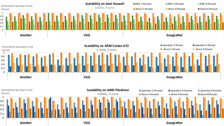
Figure 5: Scaling behavior with increasing number of threads. Our direct convolution implementation retains high GFLOPs per core performance as we increase the number of threads from 1 to the number of available cores. This is indicative of an efficient parallelized algorithm. When the number of threads exceeds the number of cores, excessive contention results in a significant drop in performance per core. In contrast, SGEMM has poor scalability even when the number of threads is low (e.g. 2).

5.3 Parallel Performance

In Figure 5, we compare the scalability of our convolution performance by parallelizing the implementation with increasing number of threads. On all architecture, we report performance per core for multi-threaded implementations normalized to the performance attained on one thread. Notice that the performance per core for existing matrix-multiplication based convolutions decrease significantly as we increase the number of threads. This is an indication that as we increase the number of threads, the processors are utilized less efficiently by the existing matrix-multiplication based implementations. Our direct CNN implementation demonstrates minimal drop in performance per core as we increase the number of threads. It is only when the number of threads is twice as much as the number of physical cores does the performance per core of our implementation drops significantly. This is expected and important as it indicates that our implementation utilizes the compute units effectively and increasing the number of threads beyond the number of physical compute units creates excessive contention for the compute resources, thereby resulting in a sharp drop in performance per core.

6 Conclusions

In this paper, we demonstrate that direct convolution, a computational technique largely ignored for computing convolution layers, is competitive with existing state of the art convolution layer computation. We show that a high performance direct convolution implementation not only eliminates all additional memory overhead, but also attains higher performance than the expert-implemented matrix-matrix-multiplication based convolution. We also show that our implementation scales to larger number of processors without degradation in performance as our implementation exploits the dimension of the kernel that has the highest amount of parallelism. In contrast, current high performance matrix-multiply based implementations do not scale as well to a larger number of processors.

Our direct convolution implementation currently attains 87.5%, 58.2% and 88.9% of the theoretical peak of the Intel, AMD, and ARM architecture, where as the SGEMM on HPC matrices attains peaks of 89% 54% and 92% the same architecture. While we have shown that our direct convolution implementation is competitive (within 3% of peak SGEMM performance), we believe that the performance gap between our direct convolution, and SGEMM on HPC matrices can be closed by taking an auto-tuning (Bilmes et al., 1997; Whaley & Dongarra, 1998) or analytical approach (Yotov et al., 2005; Low et al., 2016) to identifying the blocking parameters of the different loops. These approaches will also allow the exploration of different combinations of parallelism to determine suitable parallelism strategies. This is something we intend to pursue in the near future.

Another possible direction arising from this work is to use similar design techniques to optimize the backward process to update both in image and kernel. Given the similarity of the forward and backward process, we believe that only minor changes to the loop ordering are required.

Finally, we believe that our direct convolution algorithm can be ported to the GPU. Our proposed data layouts are similar to the layout required for the StridedBatchedGemm operation (Shi et al., 2016). As this operation and data layout is currently supported on Nvidia GPUs using cuBLAS 8.0 (Nvidia, 2017), this lends support to our belief that our algorithm can be easily ported to the GPU.

References

- Bilmes et al. (1997) Bilmes, J., Asanović, K., whye Chin, C., and Demmel, J. Optimizing matrix multiply using PHiPAC: a Portable, High-Performance, ANSI C coding methodology. In Proceedings of International Conference on Supercomputing, Vienna, Austria, July 1997.
- caffe (2) caffe2. caffe2. https://caffe2.ai/.
- Cho & Brand (2017) Cho, M. and Brand, D. MEC: memory-efficient convolution for deep neural network. CoRR, abs/1706.06873, 2017.
- Dongarra et al. (1990) Dongarra, J. J., Du Croz, J., Hammarling, S., and Duff, I. A set of level 3 basic linear algebra subprograms: Model implementation and test programs. ACM Trans. Math. Soft., 16(1):18–28, March 1990.
- (5) Dukhan, M. Nnpack. https://github.com/Maratyszcza/NNPACK.
- (6) Dundar, A., Jin, J., Gokhale, V., Krishnamurthy, B., Canziani, A., Martini, B., and Culurciello, E. Accelerating deep neural networks on mobile processor with embedded programmable logic.
- Gokhale et al. (2014) Gokhale, V., Jin, J., Dundar, A., Martini, B., and Culurciello, E. A 240 g-ops/s mobile coprocessor for deep neural networks. In Proceedings of the IEEE Conference on Computer Vision and Pattern Recognition Workshops, pp. 682–687, 2014.
- Gong et al. (2014) Gong, Y., Liu, L., Yang, M., and Bourdev, L. Compressing deep convolutional networks using vector quantization. arXiv preprint arXiv:1412.6115, 2014.
- Goto & van de Geijn (2008) Goto, K. and van de Geijn, R. Anatomy of high-performance matrix multiplication. ACM Trans. Math. Soft., 34(3):12:1–12:25, May 2008. ISSN 0098-3500.
- Gunnels et al. (2001) Gunnels, J. A., Henry, G. M., and Van De Geijn, R. A. A family of high-performance matrix multiplication algorithms. In International Conference on Computational Science, pp. 51–60. Springer, 2001.
- Han et al. (2016) Han, S., Liu, X., Mao, H., Pu, J., Pedram, A., Horowitz, M. A., and Dally, W. J. Eie: efficient inference engine on compressed deep neural network. In Proceedings of the 43rd International Symposium on Computer Architecture, pp. 243–254. IEEE Press, 2016.
- He et al. (2015) He, K., Zhang, X., Ren, S., and Sun, J. Deep residual learning for image recognition. CoRR, abs/1512.03385, 2015.
- Intel (2015) Intel. Math Kernel Library. https://software.intel.com/en-us/intel-mkl, 2015.
- Jia et al. (2014) Jia, Y., Shelhamer, E., Donahue, J., Karayev, S., Long, J., Girshick, R., Guadarrama, S., and Darrell, T. Caffe: Convolutional architecture for fast feature embedding. In Proceedings of the 22nd ACM international conference on Multimedia, pp. 675–678. ACM, 2014.
- Kim et al. (2015) Kim, Y.-D., Park, E., Yoo, S., Choi, T., Yang, L., and Shin, D. Compression of deep convolutional neural networks for fast and low power mobile applications. arXiv preprint arXiv:1511.06530, 2015.
- Krizhevsky et al. (2012) Krizhevsky, A., Sutskever, I., and Hinton, G. E. Imagenet classification with deep convolutional neural networks. In Pereira, F., Burges, C. J. C., Bottou, L., and Weinberger, K. Q. (eds.), Advances in Neural Information Processing Systems 25, pp. 1097–1105. Curran Associates, Inc., 2012.
- Lee & Verma (2013) Lee, K. H. and Verma, N. A low-power processor with configurable embedded machine-learning accelerators for high-order and adaptive analysis of medical-sensor signals. IEEE Journal of Solid-State Circuits, 48(7):1625–1637, 2013.
- Low et al. (2016) Low, T. M., Igual, F. D., Smith, T. M., and Quintana-Orti, E. S. Analytical modeling is enough for high-performance blis. ACM Transactions on Mathematical Software (TOMS), 43(2):12, 2016.
- Mathieu et al. (2013) Mathieu, M., Henaff, M., and LeCun, Y. Fast training of convolutional networks through ffts. CoRR, abs/1312.5851, 2013.
- Nvidia (2017) Nvidia. cuBLAS. https://developer.nvidia.com/cublas, 2017.
- (21) OpenBLAS. http://www.openblas.net, 2015.
- Schuster (2010) Schuster, M. Speech recognition for mobile devices at google. In Pacific Rim International Conference on Artificial Intelligence, pp. 8–10. Springer, 2010.
- Shi et al. (2016) Shi, Y., Niranjan, U. N., Anandkumar, A., and Cecka, C. Tensor contractions with extended blas kernels on cpu and gpu. In High Performance Computing (HiPC), 2016 IEEE 23rd International Conference on, pp. 193–202. IEEE, 2016.
- Simonyan & Zisserman (2014) Simonyan, K. and Zisserman, A. Very deep convolutional networks for large-scale image recognition. CoRR, abs/1409.1556, 2014.
- Smith et al. (2014) Smith, T. M., van de Geijn, R., Smelyanskiy, M., Hammond, J. R., and Zee, F. G. V. Anatomy of high-performance many-threaded matrix multiplication. In Proceedings of the 2014 IEEE 28th International Parallel and Distributed Processing Symposium, IPDPS ’14, pp. 1049–1059, Washington, DC, USA, 2014. IEEE Computer Society. ISBN 978-1-4799-3800-1. doi: 10.1109/IPDPS.2014.110. URL http://dx.doi.org/10.1109/IPDPS.2014.110.
- Szegedy et al. (2015) Szegedy, C., Liu, W., Jia, Y., Sermanet, P., Reed, S., Anguelov, D., Erhan, D., Vanhoucke, V., and Rabinovich, A. Going deeper with convolutions. In 2015 IEEE Conference on Computer Vision and Pattern Recognition (CVPR), pp. 1–9, June 2015.
- Van Zee & van de Geijn (2015) Van Zee, F. G. and van de Geijn, R. A. Blis: A framework for rapidly instantiating blas functionality. ACM Trans. Math. Softw., 41(3):14:1–14:33, June 2015. ISSN 0098-3500. doi: 10.1145/2764454. URL http://doi.acm.org/10.1145/2764454.
- Vasilache et al. (2014) Vasilache, N., Johnson, J., Mathieu, M., Chintala, S., Piantino, S., and LeCun, Y. Fast convolutional nets with fbfft: A gpu performance evaluation. arXiv preprint arXiv:1412.7580, 2014.
- Veras et al. (2016) Veras, R., Popovici, D. T., Low, T. M., and Franchetti, F. Compilers, hands-off my hands-on optimizations. In Proceedings of the 3rd Workshop on Programming Models for SIMD/Vector Processing, WPMVP ’16, pp. 4:1–4:8, New York, NY, USA, 2016. ACM. ISBN 978-1-4503-4060-1. doi: 10.1145/2870650.2870654. URL http://doi.acm.org/10.1145/2870650.2870654.
- Whaley & Dongarra (1998) Whaley, R. C. and Dongarra, J. J. Automatically tuned linear algebra software. In Proceedings of SC’98, 1998.
- Wolfe (1989) Wolfe, M. Iteration space tiling for memory hierarchies. In Proceedings of the Third SIAM Conference on Parallel Processing for Scientific Computing, pp. 357–361, Philadelphia, PA, USA, 1989. Society for Industrial and Applied Mathematics. ISBN 0-89871-228-9.
- Yotov et al. (2005) Yotov, K., Li, X., Garzarán, M. J., Padua, D., Pingali, K., and Stodghill, P. Is search really necessary to generate high-performance BLAS? Proceedings of the IEEE, special issue on “Program Generation, Optimization, and Adaptation”, 93(2), 2005.
- Zhang et al. (2014) Zhang, J., Low, T. M., Guo, Q., and Franchetti, F. A 3d-stacked memory manycore stencil accelerator system. 2014.