Local chiral interactions and magnetic structure of few-nucleon systems

Abstract

The magnetic form factors of ²H, ³H, and ³He, deuteron photodisintegration cross sections at low energies, and deuteron threshold electrodisintegration cross sections at backward angles in a wide range of momentum transfers, are calculated with the chiral two-nucleon (and three-nucleon) interactions including $\Delta$ intermediate states that have recently been constructed in configuration space. The $A\,$= 3 wave functions are obtained from hyperspherical-harmonics solutions of the Schrödinger equation. The electromagnetic current includes one- and two-body terms, the latter induced by one- and two-pion exchange (OPE and TPE, respectively) mechanisms and contact interactions. The contributions associated with $\Delta$ intermediate states are only retained at the OPE level, and are neglected in TPE loop (tree-level) corrections to two-body (three-body) current operators. Expressions for these currents are derived and regularized in configuration space for consistency with the interactions. The low-energy constants that enter the contact few-nucleon systems. The predicted form factors and deuteron electrodisintegration cross section are in excellent agreement with experiment for momentum transfers up to 2–3 fm^-1. However, the experimental values for the deuteron photodisintegration cross section are consistently underestimated by theory, unless use is made of the Siegert form of the electric dipole transition operator. A complete analysis of the results is provided, including the clarification of the origin of the aforementioned discrepancy.

I Introduction

The last few years have seen the development of chiral two-nucleon ($2N$) interactions that are local in configuration space Gezerlis:2013 ; Piarulli:2015 ; Piarulli:2016 and therefore well suited for use in quantum Monte Carlo (QMC) calculations of light-nuclei spectra and neutron-matter properties Gezerlis:2014 ; Lynn:2014 ; Lynn:2016 ; Tews:2016 ; Gandolfi:2017 ; Lynn:2017 ; Piarulli:2018 . In conjunction with these, chiral (and local) three-nucleon ($3N$) interactions have also been constructed Epelbaum:2002 ; Piarulli:2018 , and the low-energy constants (LECs) that characterize their contact terms—the LECs $c_{D}$ and $c_{E}$—have been constrained either by fitting exclusively strong-interaction observables Lynn:2016 ; Tews:2016 ; Lynn:2017 ; Piarulli:2018 or by relying on a combination of strong- and weak-interaction ones Gazit:2009 ; Marcucci:2012 ; Baroni:2018 . This last approach is made possible by the relation, established in $\chi$EFT Gardestig:2006 , between $c_{D}$ in the three-nucleon contact interaction and the LEC in the $2N$ contact axial current Gazit:2009 ; Marcucci:2012 ; Schiavilla:2017 , which allows one to use nuclear properties governed by either the strong or weak interactions to constrain simultaneously the $3N$ interaction and $2N$ axial current.

In the present study we adopt the $2N$ and $3N$ interactions constructed by our group Piarulli:2015 ; Piarulli:2016 ; Piarulli:2018 ; Baroni:2018 . The $2N$ interactions consist of an electromagnetic-interaction component, including up to quadratic terms in the fine-structure constant, and a strong-interaction component characterized by long- and short-range parts Piarulli:2015 ; Piarulli:2016 . The long-range part retains one- and two-pion exchange (respectively, OPE and TPE) terms from leading and sub-leading $\pi N$ Fettes:2000 and $\pi N\Delta$ Krebs:2007 chiral Lagrangians up to next-to-next-leading order (N2LO) in the low-energy expansion. In coordinate space, this long-range part is represented by charge-independent central, spin, and tensor components with and without isospin-dependence ${\bm{\tau}}_{i}\cdot{\bm{\tau}}_{j}$ (the so-called $v_{6}$ operator structure), and by central and tensor components induced by OPE and proportional to the isotensor operator $T_{ij}\,$=$\,3\,\tau_{i,z}\,\tau_{j,z}-{\bm{\tau}}_{i}\cdot{\bm{\tau}}_{j}$. The radial functions multiplying these operators are singular at the origin, and are regularized by a coordinate space cutoff of the form given in Eq. (23) below. The short-range part is described by charge-independent contact interactions up to N3LO, specified by a total of 20 LECs, and charge-dependent ones up to NLO, characterized by 6 LECs Piarulli:2016 . By utilizing Fierz identities, the resulting charge-independent interaction can be made to contain, in addition to the $v_{6}$ operator structure, spin-orbit, ${\bf L}^{2}$ (${\bf L}$ is the relative orbital angular momentum), and quadratic spin-orbit components, while the charge-dependent one retains central, tensor, and spin-orbit components. Both are regularized by multiplication of a Gaussian cutoff  Piarulli:2016 .

Two classes of interactions were constructed, which only differ in the range of laboratory energy over which the fits to the $2N$ database Perez:2013 were carried out, either 0–125 MeV in class I or 0–200 MeV in class II. For each class, three different sets of cutoff radii $(R_{\rm S},R_{\rm L})$ were considered $(R_{\rm S},R_{\rm L})\,$=$\,(0.8,1.2)$ fm in set a, (0.7,1.0) fm in set b, and (0.6,0.8) fm in set c. The $\chi^{2}$/datum achieved by the fits in class I (II) was $\lesssim 1.1$ $(\lesssim 1.4)$ for a total of about 2700 (3700) data points. We have been referring to these high-quality $2N$ interactions generically as the Norfolk $v_{ij}$’s (NV2s), and have been designating those in class I as NV2-Ia, NV2-Ib, and NV2-Ic, and those in class II as NV2-IIa, NV2-IIb, and NV2-IIc. Owing to the poor convergence of the hyperspherical-harmonics (HH) expansion and the severe fermion-sign problem of the Green’s function Monte Carlo (GFMC) method, however, models Ic and IIc have not been used so far in actual calculations of light nuclei.

The $3N$ interactions consist Epelbaum:2002 of a long-range piece mediated by TPE, including $\Delta$ intermediate states Piarulli:2018 , at LO and NLO, and a short-range piece parametrized in terms of two contact interactions, which enter formally at NLO, proportional to the LECs $c_{D}$ and $c_{E}$. Two distinct sets were constructed. In the first, $c_{D}$ and $c_{E}$ were determined by simultaneously reproducing the experimental trinucleon ground-state energies and $nd$ doublet scattering length for each of the $2N$ models considered, namely NV2-Ia/b and NV2-IIa/b Piarulli:2018 . In the second set, these LECs were constrained by fitting, in addition to the trinucleon energies, the empirical value of the Gamow-Teller matrix element in tritium $\beta$ decay Baroni:2018 . The resulting Hamiltonian models were designated as NV2+3-Ia/b and NV2+3-IIa/b (or Ia/b and IIa/b for short) in the first case, and as NV2+3-Ia^∗/b^∗ and NV2+3-IIa^∗/b^∗ (or Ia^∗/b^∗ and IIa^∗/b^∗) in the second. These two different procedures for fixing $c_{D}$ and $c_{E}$ produced rather different values for these LECs, particularly for $c_{E}$ which was found to be relatively large and negative in models Ia/b and IIa/b, but quite small, and not consistently negative, in models Ia^∗/b^∗ and IIa^∗/b^∗. This in turn impacts predictions for the spectra of light nuclei and the equation of state of neutron matter, since a negative $c_{E}$ leads to repulsion in light nuclei, but attraction in neutron matter. In particular, while model Ia provides an excellent description of the energy levels and level ordering of nuclei in the mass range $A\,$= 4–12 Piarulli:2018 , it collapses neutron matter already at relatively low densities Piarulli:2018a , and cannot sustain the existence of neutron stars of twice solar masses, in conflict with recent observations Demorest:2010 ; Antoniadis:2013 . By contrast, there are indications that the smaller values of $c_{E}$ characteristic of models Ia^∗/b^∗ and IIa^∗/b^∗, mitigate, if not resolve, the collapse problem, while still predicting light-nuclei spectra in reasonable agreement with experimental data Piarulli:2018a .

Electromagnetic properties of few-nucleon systems are among the observables of choice for testing models of nuclear interactions and associated electromagnetic charge and current operators. Nuclear electromagnetic charge and current operators in a $\chi$EFT formulation with nucleon and pion degrees of freedom were derived up to one loop originally by Park et al. Park:1993 ; Park:1996 in covariant perturbation theory. Subsequently, two independent derivations, based on time-ordered perturbation theory (TOPT), appeared in the literature, one by some of the present authors Pastore:2009 ; Pastore:2011 ; Piarulli:2013 and the other by Kölling et al. Koelling:2009 ; Koelling:2011 . These two derivations differ in the way in which non-iterative terms are isolated in reducible contributions. The authors of Refs. Koelling:2009 ; Koelling:2011 use TOPT in combination with the unitary transformation method Okubo:1954 to decouple, in the Hilbert space of pions and nucleons, the states consisting of nucleons only from those including, in addition, pions. In contrast, we construct an interaction such that, when iterated in the Lippmann-Schwinger equation, generates a $T$-matrix matching, order by order in the power counting, the $\chi$EFT amplitude calculated in TOPT Pastore:2011 ; Pastore:2008 . These two different formulations lead to the same formal expressions for the electromagnetic current operator up to one loop (or N3LO). However, some differences remain in the electromagnetic charge operator, specifically in some of the pion-loop corrections to its short-range part Piarulli:2013 . They are not relevant here (and will not be discussed any further), since we are primarily interested in magnetic structure and response.

A partial derivation of the electromagnetic current in a $\chi$EFT formulation which explicitly accounts for $\Delta$ intermediate states in TPE contributions was carried out in Ref. Pastore:2008 . However, a systematic study of these contributions in two-body (as well as three-body) currents is not yet available (within $\chi$EFT). In the present work, we only retain $\Delta$ contributions at the OPE level, which formally enter at N2LO in the chiral expansion, and ignore altogether their contributions to TPE mechanisms at N3LO. There are indications from an earlier study Marcucci:1998 which approximately accounted for explicit $\Delta$ components in nuclear ground states with the transition-correlation-operator method Schiavilla:1992 , that the latter are much smaller than the former in the low-momentum transfer region of the trinucleon magnetic form factors of interest here (see Figs. 13–14 and 18–19 of Ref. Marcucci:1998 ). Thus, we do not expect the present incomplete treatment of $\Delta$ effects to significantly affect our predictions for the two- and three-body observables we consider here.

This paper is organized as follows. In Sec. II we list explicitly the configuration-space expressions for the electromagnetic current up to N3LO. Those up to N2LO are well known, and are reported here for completeness and clarity of presentation. However, the configuration-space expressions for the loop corrections at N3LO were, to the best of our knowledge, not previously known; they are derived in Appendix A of the present paper. In Sec. III we determine the unknown LECs that enter the current at N3LO by fitting the magnetic moments of ²H, ³H, and ³He for each of the Hamiltonian models considered (Ia^∗/b^∗ and IIa^∗/b^∗), and in Sec. IV present predictions for the magnetic form factors of these nuclei, the deuteron photodisintegration cross section for photon energies ranging from threshold up to 30 MeV, and the deuteron threshold electrodisintegration cross section at backward angles for momentum transfers up to about 5.5 fm^-1 corresponding to these models (as well as models Ia/b and IIa/b for the trinucleon form factors), along with a fairly detailed analysis of these results. Finally, we offer some concluding remarks in Sec. V.

II Electromagnetic current up to N3LO

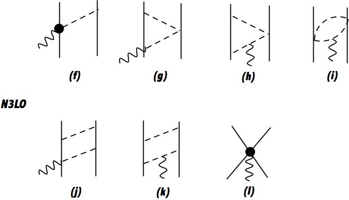
Figure 2: Diagrams illustrating the contributions to the electromagnetic current at N3LO (with power scaling $Q$) without the inclusion of $\Delta$ intermediate states. Nucleons, pions, and external fields are denoted by solid, dashed, and wavy lines, respectively. The solid circle in panel (f) is associated with $\gamma\pi N$ interaction vertices generated by ${\cal L}^{(3)}_{\pi N}$ Fettes:2000 .

We illustrate the contributions to the two-body electromagnetic current in a $\chi$EFT with nucleon, $\Delta$-isobar, and pion degrees of freedom up to N2LO in Fig. 1, and the contributions at N3LO excluding $\Delta$ intermediate states in Fig. 2. They have been derived in a number of papers in approaches based on either covariant perturbation theory Park:1993 ; Park:1996 or, more recently, time-ordered perturbation theory Pastore:2009 ; Koelling:2009 ; Pastore:2011 ; Koelling:2011 ; Piarulli:2013 . For completeness and ease of presentation, we report below the configuration-space expressions of these various terms.

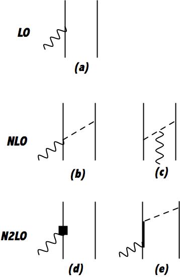
Figure 1: Diagrams illustrating the contributions to the electromagnetic current up to N2LO (with power scaling up to $Q^{0}$). Nucleons, $\Delta$-isobars, pions, and external fields are denoted by solid, thick-solid, dashed, and wavy lines, respectively. The square in panel (d) represents relativistic corrections to the LO current. Only a single time ordering is shown in panels (b), (c), and (e).

The LO one in panel (a), which scales as $Q^{-2}$ in the power counting ($Q$ denotes generically a low-momentum scale), reads

$${\bf j}^{\rm LO}({\bf q})=\frac{\epsilon_{i}}{2\,m}\,\left\{{\bf p}_{i}\,\,,\,\,{\rm e}^{i{\bf q}\cdot{\bf r}_{i}}\right\}+i\,\frac{\mu_{i}}{2\,m}\,\,{\rm e}^{i{\bf q}\cdot{\bf r}_{i}}\,\,{\bm{\sigma}}_{i}\times{\bf q}\,+(i\rightleftharpoons j)\ ,$$ (1)

where ${\bf p}_{k}\,$=$\,-i\,{\bm{\nabla}}_{k}$ and ${\bm{\sigma}}_{k}$ are the momentum and Pauli spin operators of nucleon $k$, $m$ is its mass ($m\,$= 938.9 MeV), ${\bf q}$ is the external field momentum, and we have defined the isospin operators

$$\epsilon_{k} = (1+\tau_{k,z})/2\ ,\qquad\mu_{k}=(\mu^{S}+\mu^{V}\tau_{k,z})/2\ .$$ (2)

Here $\mu^{S}$ and $\mu^{V}$ are the isoscalar and isovector combinations of the nucleon magnetic moments ($\mu^{S}\,$=$\,0.8798$ n.m. and $\mu^{V}\,$=$\,4.7059$ n.m.). The NLO terms in panels (b) and (c) with scaling $Q^{-1}$ are written as

$${\bf j}^{\rm NLO}({\bf q}) = \left[{\rm e}^{i\,{\bf q}\cdot{\bf r}_{i}}\,\left({\bm{\tau}}_{i}\times{\bm{\tau}}_{j}\right)_{z}\,I_{0}^{\pi}(\mu_{ij})\,{\bm{\sigma}}_{i}\,\,{\bm{\sigma}}_{j}\cdot\hat{\bf r}_{ij}+\!(i\rightleftharpoons j)\right]+\,{\rm e}^{i\,{\bf q}\cdot{\bf R}_{ij}}\,\left({\bm{\tau}}_{i}\times{\bm{\tau}}_{j}\right)_{z}\,\,{\bm{\sigma}}_{i}\cdot\left({\bm{\nabla}}^{\mu}_{ij}+i\,\frac{\bf q}{2\,m_{\pi}}\right)$$ (3)

$$\times{\bm{\sigma}}_{j}\cdot\left({\bm{\nabla}}_{ij}^{\mu}-i\,\frac{\bf q}{2\,m_{\pi}}\right){\bm{\nabla}}^{\mu}_{ij}\,L_{0}^{\pi}({\bm{\mu}}_{ij},{\bf q})\ ,$$

where

$${\bf r}_{ij}={\bf r}_{i}-{\bf r}_{j}\ ,\qquad{\bf R}_{ij}=\left({\bf r}_{i}+{\bf r}_{j}\right)/2\ ,\qquad{\bm{\mu}}_{ij}=m_{\pi}\,{\bf r}_{ij}\ ,$$ (4)

the gradients ${\bm{\nabla}}^{\mu}_{ij}$ are relative to the adimensional variables ${\bm{\mu}}_{ij}$, and the correlation functions $I_{0}^{\pi}(\mu)$ and $L_{0}^{\pi}({\bm{\mu}},{\bf q})$ are defined as

$$I_{0}^{\pi}(\mu) = -\frac{g^{2}_{A}}{16\,\pi}\,\frac{m_{\pi}^{2}}{f_{\pi}^{2}}\,(1+\mu)\,\frac{e^{-\mu}}{\mu^{2}}\ ,$$ (5)

$$L_{0}^{\pi}({\bm{\mu}},{\bf q}) = \frac{g^{2}_{A}}{16\,\pi}\,\frac{m_{\pi}^{2}}{f_{\pi}^{2}}\int_{-1/2}^{1/2}dz\,\,{\rm e}^{-i\,z\left({\bf q}/m_{\pi}\right)\cdot{\bm{\mu}}}\,\,\frac{e^{-\mu\,L(z,q)}}{L(z,q)}\ ,$$ (6)

with

$$L(z,q)=\sqrt{1+\frac{q^{2}}{4\,m_{\pi}^{2}}\left(1-4\,z^{2}\right)}\ ,$$ (7)

and $g_{A}$ and $f_{\pi}$ are, respectively, the nucleon axial coupling constant ($g_{A}\,$=$\,1.29$) and pion-decay amplitude ($f_{\pi}\,$=$\,92.4$ MeV), and $m_{\pi}$ is average pion mass ($m_{\pi}\,$= 138.039 MeV) (these values are taken from Ref. Piarulli:2015 ). The N2LO terms (with scaling $Q^{0}$) consist of relativistic corrections (RC) to the LO current, panel (d), and contributions involving $\Delta$ intermediate states ($\Delta$), panel (e),

$${\bf j}^{\rm N2LO}_{\rm RC}({\bf q}) = -\frac{\epsilon_{i}}{16\,m^{3}}\left\{2\left(p_{i}^{2}+\frac{q^{2}}{4}\right)\big{(}2\,{\bf p}_{i}+i\,{\bm{\sigma}}_{i}\times{\bf q}\big{)}+{\bf p}_{i}\cdot{\bf q}\,\left({\bf q}+2\,i\,{\bm{\sigma}}_{i}\times{\bf p}_{i}\right)\,\,,\,\,{\rm e}^{i{\bf q}\cdot{\bf r}_{i}}\right\}$$ (8)

$$-i\,\frac{\mu_{i}-\epsilon_{i}}{16\,m^{3}}\left\{{\bf p}_{i}\cdot{\bf q}\big{(}4\,{\bm{\sigma}}_{i}\times{\bf p}_{i}-i\,{\bf q}\big{)}-\left(2\,i\,{\bf p}_{i}-{\bm{\sigma}}_{i}\times{\bf q}\right)\frac{q^{2}}{2}+2\,\left({\bf p}_{i}\times{\bf q}\right)\,{\bm{\sigma}}_{i}\cdot{\bf p}_{i}\,\,,\,\,{\rm e}^{i{\bf q}\cdot{\bf r}_{i}}\right\}+(i\rightleftharpoons j)\ ,$$

$${\bf j}^{\rm N2LO}_{\Delta}({\bf q}) = -i\,{\rm e}^{i{\bf q}\cdot{\bf r}_{i}}\,\tau_{j,z}\left[I^{\Delta}_{1}(\mu_{ij})\,{\bm{\sigma}}_{j}+I_{2}^{\Delta}(\mu_{ij})\,\,{\bm{\sigma}}_{j}\cdot\hat{\bf r}_{ij}\,\,\hat{\bf r}_{ij}\right]\times\frac{{\bf q}}{m_{\pi}}$$ (9)

$$+\frac{i}{4}\,{\rm e}^{i\,{\bf q}\cdot{\bf r}_{i}}\,\left({\bm{\tau}}_{i}\times{\bm{\tau}}_{j}\right)_{z}\left[I^{\Delta}_{1}(\mu_{ij})\,{\bm{\sigma}}_{i}\times{\bm{\sigma}}_{j}+I^{\Delta}_{2}(\mu_{ij})\,{\bm{\sigma}}_{j}\cdot\hat{\bf r}_{ij}\,\,{\bm{\sigma}}_{i}\times\hat{\bf r}_{ij}\right]\times\frac{{\bf q}}{m_{\pi}}+(i\rightleftharpoons j)\ ,$$

where the correlation functions $I^{\Delta}_{k}(\mu)$ are

$$I^{\Delta}_{1}(\mu) = -\left(\frac{g_{A}\,h_{A}}{18\,\pi}\,\frac{\mu_{\Delta N}}{2\,m}\,\frac{m_{\pi}^{2}}{m_{\Delta N}}\frac{m_{\pi}^{2}}{f_{\pi}^{2}}\right)(1+\mu)\,\frac{e^{-\mu}}{\mu^{3}}\ ,$$ (10)

$$I^{\Delta}_{2}(\mu) = \left(\frac{g_{A}\,h_{A}}{18\,\pi}\,\frac{\mu_{\Delta N}}{2\,m}\,\frac{m_{\pi}^{2}}{m_{\Delta N}}\frac{m_{\pi}^{2}}{f_{\pi}^{2}}\right)(3+3\,\mu+\mu^{2})\,\frac{e^{-\mu}}{\mu^{3}}\ ,$$ (11)

and $h_{A}$ and $\mu_{\Delta N}$ are, respectively, the nucleon-to-$\Delta$ transition axial coupling constant ($h_{A}\,$= 2.74) and magnetic moment ($\mu_{\Delta N}\,$= 3 n.m. Carlson:1986 ), and $m_{\Delta N}$ is $\Delta$-nucleon mass difference ($m_{\Delta N}\,$= 293.1 MeV). The N3LO terms are written as the sum of an isoscalar OPE contribution, panel (f),

$${\bf j}^{\rm N3LO}_{\rm OPE}({\bf q})=-i\,{\rm e}^{i{\bf q}\cdot{\bf r}_{i}}\,{\bm{\tau}}_{i}\cdot{\bm{\tau}}_{j}\left[I^{\pi}_{1}(\mu_{ij})\,{\bm{\sigma}}_{j}+I^{\pi}_{2}(\mu_{ij})\,\,{\bm{\sigma}}_{j}\cdot\hat{\bf r}_{ij}\,\,\hat{\bf r}_{ij}\right]\times\frac{{\bf q}}{m_{\pi}}+(i\rightleftharpoons j)\ ,$$ (12)

isovector TPE contributions, panels (g)-(k),

$${\bf j}^{{\rm N3LO}}_{\rm TPE}({\bf q}) = i\,\tau_{j,z}\,\,{\rm e}^{i{\bf q}\cdot{\bf R}_{ij}}\left\{\left[F^{(0)}_{0}(\lambda_{ij})+F^{(1)}_{2}(\lambda_{ij})\right]{\bm{\sigma}}_{i}+F^{(2)}_{2}(\lambda_{ij})\,{\bm{\sigma}}_{i}\cdot\hat{\bf r}_{ij}\,\,\hat{\bf r}_{ij}\right\}\times\frac{{\bf q}}{2\,m_{\pi}}$$ (13)

$$-\frac{1}{2}({\bm{\tau}}_{i}\times{\bm{\tau}}_{j})_{z}\,\,{\rm e}^{i{\bf q}\cdot{\bf R}_{ij}}\,\hat{\bf r}_{ij}\,\left[\lambda_{ij}\,\frac{v^{\rm NLO}_{\,2\pi}(\lambda_{ij})}{2\,m_{\pi}}\right]+(i\rightleftharpoons j)\ ,$$

and both isoscalar and isovector contact contributions, panel (l), from minimal (MIN) and non-minimal (NM) couplings and from the regularization scheme in configuration space we have adopted for the TPE current (and labeled CT) in Appendix A, respectively,

$${\bf j}^{\rm N3LO}_{\rm MIN}({\bf q}) = \frac{1}{8}\,\,\left({\bm{\tau}}_{i}\times{\bm{\tau}}_{j}\right)_{z}\,\,{\rm e}^{i{\bf q}\cdot{\bf R}_{ij}}\ C^{(1)}_{R_{\rm S}}(z_{ij})\Big{[}\,m_{\pi}^{4}\left(C_{2}+3\,C_{4}+C_{7}\right)\hat{\bf r}_{ij}+m_{\pi}^{4}\left(C_{2}-C_{4}-C_{7}\right)\,\hat{\bf r}_{ij}\,\,{\bm{\sigma}}_{i}\cdot{\bm{\sigma}}_{j}$$ (14)

$$+\,m_{\pi}^{4}\,C_{7}\left({\bm{\sigma}}_{i}\cdot\hat{\bf r}_{ij}\,\,{\bm{\sigma}}_{j}+{\bm{\sigma}}_{j}\cdot\hat{\bf r}_{ij}\,\,{\bm{\sigma}}_{i}\right)\Big{]}-\frac{1}{8}m_{\pi}^{4}\,C_{5}\,{\rm e}^{i{\bf q}\cdot{\bf R}_{ij}}\Big{[}\left(\tau_{i,z}-\tau_{j,z}\right)\,C^{(1)}_{R_{\rm S}}(z_{ij})\left({\bm{\sigma}}_{i}+{\bm{\sigma}}_{j}\right)\times\hat{\bf r}_{ij}$$

$$+\,i\,C^{(0)}_{R_{\rm S}}(z_{ij})\left({\bm{\sigma}}_{i}+{\bm{\sigma}}_{j}\right)\times\frac{\bf q}{m_{\pi}}\Big{]}\ ,$$

$${\bf j}^{\rm N3LO}_{\rm NM}({\bf q}) = -i\,{\rm e}^{i{\bf q}\cdot{\bf R}_{ij}}\,C^{(0)}_{R_{\rm S}}(z_{ij})\Big{[}m_{\pi}^{4}\,C_{15}^{\prime}\left({\bm{\sigma}}_{i}+{\bm{\sigma}}_{j}\right)+m_{\pi}^{4}\,C_{16}^{\prime}\,(\tau_{i,z}-\tau_{j,z})\left({\bm{\sigma}}_{i}-{\bm{\sigma}}_{j}\right)\Big{]}\,\times\frac{{\bf q}}{m_{\pi}}\ ,$$ (15)

$${\bf j}^{{\rm N3LO}}_{\rm CT}({\bf q}) = i\,\tau_{j,z}\,\,{\rm e}^{i{\bf q}\cdot{\bf R}_{ij}}\,\,F^{(0)}_{0}(z_{ij};\infty)\,\,{\bm{\sigma}}_{i}\times\frac{{\bf q}}{2\,m_{\pi}}+(i\rightleftharpoons j)\ ,$$ (16)

where we have introduced the notation

$$\lambda_{ij}=2\,m_{\pi}\,r_{ij}\ ,\qquad z_{ij}=r_{ij}/R_{\rm S}\ ,$$ (17)

and in the contact terms the $\delta$-function has been smeared by a Gaussian cutoff and hence

$$C^{(0)}_{R_{\rm S}}(z)=\frac{1}{\pi^{3/2}\,(m_{\pi}\,R_{\rm S})^{3}}\,{\rm e}^{-z^{2}}\ ,\qquad C^{(1)}_{R_{\rm S}}(z)=\frac{1}{m_{\pi}\,R_{\rm S}}\,\frac{d\,C^{(0)}_{R_{\rm S}}(z)}{dz}\ .$$ (18)

The correlation functions $I^{\pi}_{1}(\mu)$ and $I^{\pi}_{2}(\mu)$ in Eq. (12) are defined as in Eqs. (10) and (11), but for the combination of constants in front of those equations being replaced by

$$\left(\frac{g_{A}\,h_{A}}{18\,\pi}\,\frac{\mu_{\Delta N}}{2\,m}\,\frac{m_{\pi}^{2}}{m_{\Delta N}}\frac{m_{\pi}^{2}}{f_{\pi}^{2}}\right)\longrightarrow\left(\frac{g_{A}}{16\,\pi}\,\frac{m_{\pi}^{2}}{f_{\pi}^{2}}\,m_{\pi}^{2}\,d_{9}^{\prime}\right)\ .$$ (19)

The derivation of the loop correlation functions $F_{0}^{(0)}(z_{ij};\infty)$, $F_{0}^{(0)}(\lambda)$, $F_{2}^{(1)}(\lambda)$, and $F_{2}^{(2)}(\lambda)$ is somewhat involved and is relegated in Appendix A—the relevant equations, where these functions are defined, are (60), (A.2), and (83)–(84), respectively.

Several comments are now in order. First, we have not accounted for explicit $\Delta$ intermediate states in the corrections at N3LO. These enter in loops in two-body operators—indeed, a partial derivation of them was already given in Ref. Pastore:2008 —and at tree-level in three-body operators (note that there are no such terms at N3LO in a $\chi$EFT with nucleon and pion degrees of freedom only Girlanda:2010 ). Indeed, contributions due to these higher-order $\Delta$ currents have yet to be studied quantitatively in calculations of electro- and photo-nuclear observables. In this context, we also note that the isovector OPE current at N3LO from the Lagrangian ${\cal L}^{(3)}_{\pi N}$ Fettes:2000 , which depends on the LECs $d_{8}^{\prime}$ and $d_{21}^{\prime}$ in the notation of Ref. Piarulli:2013 , has been assumed here to be saturated by the three-level $\Delta$ current of panel (e).

Second, the longitudinal term in the loop corrections of Eq. (13) involves the TPE interaction $v_{2\pi,ij}^{\rm NLO}\!=\!v_{2\pi}^{\rm NLO}(r_{ij})\,{\bm{\tau}}_{i}\cdot{\bm{\tau}}_{j}$ which one obtains at NLO Pastore:2009 ; Piarulli:2013 (with nucleons and pions only). However, the chiral interactions adopted in the present study receive TPE contributions also from $\Delta$ intermediate states at both NLO and N2LO Piarulli:2016 ; as a matter of fact, up to N2LO included, they have the following operator structure Piarulli:2015 ; Piarulli:2016

$$\widetilde{v}_{2\pi,ij}^{\,\rm N2LO}=\sum_{p=1}^{6}\widetilde{v}_{\,2\pi}^{\,(p)}(r_{ij})\,O^{(p)}_{ij}\ ,\qquad O^{(p=1,\dots,6)}_{ij}=\left[{\bf 1}\,,\,{\bm{\sigma}}_{i}\cdot{\bm{\sigma}}_{j}\,,\,S_{ij}\right]\otimes\left[{\bf 1}\,,\,{\bm{\tau}}_{i}\cdot{\bm{\tau}}_{j}\right]\ ,$$ (20)

where $S_{ij}$ is the standard tensor operator. Hereafter, we will make the replacement

$$v_{2\pi}^{\rm NLO}(r_{ij})\longrightarrow\widetilde{v}_{\,2\pi}^{\,(2)}(r_{ij})+\widetilde{v}_{\,2\pi}^{\,(4)}(r_{ij})\,\,{\bm{\sigma}}_{i}\cdot{\bm{\sigma}}_{j}+\widetilde{v}_{\,2\pi}^{\,(6)}(r_{ij})\,\,S_{ij}$$ (21)

in the longitudinal term of Eq. (13), where $\widetilde{v}_{\,2\pi}^{\,(p)}(r_{ij})\,O^{(p)}_{ij}$ with $p$ even denote the isospin-dependent central, spin-spin, and tensor components. While such a replacement is not consistent from a power-counting perspective, it ensures, nevertheless, that the resulting TPE current satisfies the continuity equation (with the corresponding interaction components) in the limit of small momentum transfers, see Appendix A.

Third, in the contact terms the LECs $C_{i}$ are taken from Ref. Piarulli:2016 , where they have been determined by fits to $pp$ and $np$ cross sections and polarization observables, including $pp$, $np$, and $nn$ scattering lengths and effective ranges. The determination of the LECs $C_{15}^{\prime}$ and $C_{16}^{\prime}$ in the non-minimal current, and $d_{9}^{\prime}$ in the isoscalar OPE current at N3LO, is discussed in the following section.

Finally, the OPE and TPE correlation functions as well as the OPE ones resulting from the application of the gradients to $L_{0}^{\pi}(\mu)$, denoted generically with $X(m_{\pi}r)$ below, are each regularized by multiplication of a configuration-space cutoff as in the case of the local chiral interactions of Refs. Piarulli:2015 ; Piarulli:2016 ; Baroni:2018 , namely

$$X(m_{\pi}r)\longrightarrow C_{R_{\rm L}}(r)\,X(m_{\pi}r)\ ,$$ (22)

with

$$C_{R_{\rm L}}(r)=1-\frac{1}{\left(r/R_{\rm L}\right)^{p}\,{\rm e}^{(r-R_{\rm L})/a_{\rm L}}+1}\ ,$$ (23)

where $a_{\rm L}\,$=$\,R_{\rm L}/2$, and the exponent $p$ is taken as $p\,$=$\,6$ for consistency with the interactions (note that the correlation functions in the TPE currents behave as ${\rm ln}\,r/r^{3}$ in the limit $r\rightarrow 0$).

III Determination of low-energy constants

As already mentioned, the LECs $C_{i}$, $i=1,\dots,7$, in the minimal contact current are taken from fits to nucleon-nucleon scattering data Piarulli:2016 . In reference to the LECs entering the OPE and non-minimal contact currents at N3LO, it is convenient to introduce the adimensional set $d_{i}^{S,V}$ (in units of $m_{\pi}$) as

$$C_{15}^{\prime}=d_{1}^{S}/m_{\pi}^{4}\ ,\qquad d_{9}^{\prime}=d_{2}^{S}/m_{\pi}^{2}\ ,\qquad C_{16}^{\prime}=d_{1}^{V}/m_{\pi}^{4}\ ,$$ (24)

where the superscript $S$ or $V$ on the $d^{S,V}_{i}$ characterizes the isospin of the associated operator, i.e., whether it is isoscalar or isovector. The values of these LECs are listed in Table 1: $d_{1}^{S}$ and $d_{2}^{S}$ have been fixed by reproducing the experimental deuteron magnetic moment $\mu_{d}$ and isoscalar combination $\mu_{S}$ of the trinucleon magnetic moments, while $d_{1}^{V}$ has been determined by their isovector combination. Naive power counting would indicate that the values for these LECs are natural. Indeed, since the NLO and N3LO non-minimal (NM) contact contributions scale as (hereafter, the low momentum scale $Q$ is assumed to be of order $m_{\pi}$)

$${\rm NLO}\sim\frac{g_{A}^{2}}{4\,f_{\pi}^{2}}\,\frac{1}{m_{\pi}}\ ,\qquad{\rm N3LO(NM)}\sim\frac{1}{m^{3}_{\pi}}\,d_{1}^{S,V}\ ,$$ (25)

and since the ratio ${\rm N3LO(NM)}/{\rm NLO}$ is expected to be suppressed by $m^{2}_{\pi}/\Lambda_{\chi}^{2}$, where $\Lambda_{\chi}$ is the hard scale which we take as $\Lambda_{\chi}\,$$\sim$ 1 GeV, it follows that

$$d_{1}^{S,V}\sim\frac{g_{A}^{2}}{4}\,\frac{m_{\pi}^{2}}{f_{\pi}^{2}}\,\frac{m_{\pi}^{2}}{\Lambda_{\chi}^{2}}\sim 0.018\ .$$ (26)

A similar argument leads to the expectation that the LEC in the OPE (isoscalar) contribution at N3LO has a magnitude of the order

$$d_{2}^{S}\sim g_{A}\,\frac{m_{\pi}^{2}}{\Lambda_{\chi}^{2}}\sim 0.025\ .$$ (27)

Both these values are not out of line with those reported in Table 1.

	Ia∗	Ib∗	IIa∗	IIb∗
$d_{1}^{S}$	$-0.009\,99$	$-0.025\,11$	$-0.011\,70$	$-0.049\,55$
$d_{2}^{S}$	$-0.065\,71$	$-0.023\,84$	$-0.047\,14$	$-0.079\,47$
$d_{1}^{V}$	$-0.051\,20$	$-0.035\,09$	$-0.051\,28$	$-0.038\,80$

Table 1: Adimensional values of the isoscalar and isovector LECs corresponding to the nuclear Hamiltonians NV2+3-Ia^∗/b^∗ and NV2+3-IIa^∗/b^∗ Baroni:2018 , designated as Ia^∗/b^∗ and IIa^∗/b^∗ for brevity.

The calculations of the observables are based on the (chiral) two-nucleon interactions of Ref. Piarulli:2016 for the deuteron, augmented by the (chiral) three-nucleon interactions developed in Refs. Piarulli:2018 ; Baroni:2018 for ³He/³H, and use, for the trinucleon case, wave functions obtained from hyperspherical-harmonics (HH) solutions of the Schrödinger equation with these interactions (see Ref. Kievsky:2008 for a review of HH methods). The corresponding Hamiltonians are denoted as NV2+3-Ia^∗/b^∗ and NV2+3-IIa^∗/b^∗ (or Ia^∗/b^∗ and IIa^∗/b^∗ for short), where I or II, and a or b, specify, respectively, the energy range over which the fits to the two-nucleon database were carried out (for the two-nucleon interactions Piarulli:2016 )—either 0–125 MeV (I) or 0–200 MeV (II)—and the set of cutoff radii $(R_{\rm S},R_{\rm L})$ considered—either (0.8,1.2) fm (a) or (0.7,1.0) fm (b). In combination with each of these, the LECs $c_{D}$ and $c_{E}$ that characterize the contact terms in the three-nucleon interaction Piarulli:2018 have been constrained by fitting the trinucleon binding energies and Gamow-Teller matrix element contributing to tritium $\beta$ decay Baroni:2018 . We note that in an earlier version of these three-nucleon interactions, rather than the Gamow-Teller matrix element, the neutron-deuteron doublet scattering length had been reproduced Piarulli:2018 . The corresponding Hamiltonians, designated as NV2+3-Ia/b and NV2+3-IIa/b (or simply Ia/b and IIa/b), will also be used below in some cases.

	Eqs.
LO	(1)
NLO	(3)
N2LO(RC)	(8)
N2LO($\Delta$)	(9)
N3LO(LOOP)	(13)+(16)
N3LO(MIN)	(14)
N3LO(NM)	(15)
N3LO(OPE)	(12)

Table 2: Notation adopted for the various terms in the current operator; N2LO and N3LO denote respectively the sum of all terms at N2LO and N3LO.

Magnetic form factors and magnetic moments of spin $J\,$=1/2 and 1 systems can be obtained by evaluating the matrix element Carlson:2015

$$F_{M}(q;A)=-i\,\frac{2\,m}{q}\,\langle A;JJ|j_{y}(q\,\hat{\bf x})|A;JJ\rangle\ ,\qquad\mu_{A}=F_{M}(0;A)\ ,$$ (28)

where $|A;JJ\rangle$ represents the ground state of the nucleus $|A;JM_{J}\rangle$ in the stretched configuration having $M_{J}\,$=$\,J$, and $j_{y}(q\,\hat{\bf x})$ is the $y$-component of the current operator with the momentum transfer ${\bf q}$ taken in the $x$-direction. Both $A\,$=2 and 3 matrix elements of interest here have been calculated by Monte Carlo integration techniques based on the Metropolis algorithm Metropolis:1953 and utilizing random walks with, respectively, $\sim\,$$10^{6}$ and $\sim\,$$\,5\times 10^{5}$ samples (see Ref. Carlson:2015 for a recent review of Monte Carlo methods as applied in nuclear physics). Statistical errors are typically well below 1% for each individual contribution to the current (in fact, at the level of a few parts in $10^{4}$ for the LO and, typically, a few parts in $10^{3}$ for the higher orders), and will not be quoted in the results reported below unless explicitly noted.

	Ia∗	Ib∗	IIa∗	IIb∗
LO	$0.8498$	$0.8485$	$0.8501$	$0.8501$
N2LO(RC)	$-0.0062$	$-0.0061$	$-0.0065$	$-0.0072$
N3LO(MIN)	$0.0002$	$0.0005$	$0.0002$	$0.0009$
N3LO(NM)	$0.0093$	$0.0211$	$0.0110$	$0.0396$
N3LO(OPE)	$0.0042$	$-0.0065$	$0.0026$	$-0.0260$

Table 3: Individual contributions to the deuteron magnetic moment in units of n.m., corresponding to the nuclear Hamiltonians Ia^∗/b^∗ and IIa^∗/b^∗. The experimental value is $0.8574$ n.m., and is reproduced by adding all contributions.

Individual contributions, associated with the various terms as designated in Table 2, to $\mu_{d}$, and $\mu_{S}$ and $\mu_{V}$, are reported in Tables 3 and 4, respectively. The NLO and N3LO(LOOP) current operators are isovector, and therefore do not contribute to isoscalar observables, such as $\mu_{d}$ (and the deuteron magnetic form factor, see below). At N3LO the only non-vanishing contributions to isoscalar observables are those from the OPE and minimal (MIN) and NM contact currents. Note, however, that since the HH trinucleon wave functions include components with total isospin 3/2 induced by isospin-symmetry-breaking terms from strong and electromagnetic interactions, purely isovector current operators—specifically, those at NLO, N2LO($\Delta$), and N3LO(LOOP)—give tiny contributions to $\mu_{S}$; conversely, the purely isoscalar current operator N3LO(OPE) gives a tiny contribution to $\mu_{V}$. Lastly, the sums of all contributions in Tables 3 and 4 reproduce (by design) the experimental values for $\mu_{d}$, and $\mu_{S}$ and $\mu_{V}$.

	$\mu_{S}$				$\mu_{V}$
	Ia∗	Ib∗	IIa∗	IIb∗	Ia∗	Ib∗	IIa∗	IIb∗
LO	$0.4089$	$0.4075$	$0.4091$	$0.4089$	$-2.1823$	$-2.1755$	$-2.1815$	$-2.1787$
NLO	$0.0015$	$0.0020$	$0.0012$	$0.0018$	$-0.1967$	$-0.2257$	$-0.1967$	$-0.2255$
N2LO	$-0.0062$	$-0.0043$	$-0.0052$	$-0.0071$	$-0.0388$	$-0.0657$	$-0.0395$	$-0.0617$
N3LO(LOOP)	$0.0004$	$0.0004$	$0.0003$	$0.0002$	$-0.0290$	$-0.0233$	$-0.0287$	$-0.0205$
N3LO(MIN)	$0.0001$	$0.0005$	$0.0002$	$0.0010$	$0.0035$	$0.0038$	$0.0033$	$0.0035$
N3LO(NM)	$0.0130$	$0.0269$	$0.0148$	$0.0488$	$-0.1098$	$-0.0668$	$-0.1100$	$-0.0704$
N3LO(OPE)	$0.0094$	$-0.0063$	$0.0065$	$-0.0269$	$-0.0002$	$-0.0001$	$0.0000$	$0.0002$

Table 4: Individual contributions to the isoscalar and isovector combinations of the trinucleon magnetic moments in units of n.m., corresponding to the nuclear Hamiltonians Ia^∗/b^∗ and IIa^∗/b^∗. The experimental values are $0.4257$ n.n. and $-2.553$ n.m., respectively, and are reproduced by adding all contributions.

As it can be surmised from the difference between models a and b in both classes I and II, the LO contribution to the $A\,$= 2 and 3 magnetic moments is very weakly dependent on the pair of cutoff radii $(R_{\rm S},R_{\rm L})$ characterizing the two- and three-nucleon interactions from which the ²H, and ³H and ³He wave functions are derived. In contrast the cutoff dependence is much more pronounced in the case of the N2LO($\Delta$) and N3LO contributions, since for these the short- and long-range regulators directly enter the correlation functions of the corresponding transition operators. This cutoff dependence is in turn reflected in the significant variation of the LECs $d_{i}^{S}$ and $d_{1}^{V}$ between models a and b. The N2LO(RC) correction, which is nominally suppressed by two powers of the expansion parameter $Q/\Lambda_{\chi}$, being inversely proportional to the cube of the nucleon mass, itself of order $\Lambda_{\chi}$, is in fact further suppressed than the naive N2LO power counting would imply; as a matter of fact, it is typically an order of magnitude smaller than the N2LO($\Delta$) contribution.

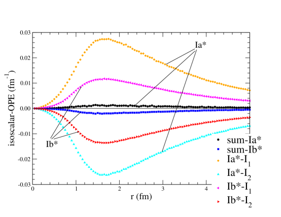
Figure 3: (Color online). The “densities” relative to $\mu_{d}$ and corresponding to the terms proportional to $I_{1}^{\pi}$ and $I_{2}^{\pi}$ in the N3LO(OPE) current of Eq. (12) (curves labeled $I_{1}$ and $I_{2}$) as well to the full current (curve labeled “sum”), shown as functions of the internucleon separation $r$ for models Ia^∗ and Ib^∗.

The isoscalar N3LO(OPE) contribution to $\mu_{d}$ and $\mu_{S}$ exhibits the most striking cutoff dependence—it changes sign in going from models a^∗ to b^∗. The origin of this dependence becomes apparent when the contributions of the terms proportional to the correlation functions $I_{1}^{\pi}(\mu)$ and $I_{2}^{\pi}(\mu)$ in the matrix element of the ${\bf j}^{\rm N3LO}_{\rm OPE}$ current are calculated independently: they turn out to be large and of opposite sign. In Fig. 3 we show the “densities”, as functions of the relative distance $r$ between the two nucleons, associated with these terms (curves labeled $I_{1}$ and $I_{2}$) as well as with their sum for the deuteron magnetic moment matrix element—integration over $r$ gives the corresponding contribution, in particular integration of the curve labeled “sum” leads to the full N3LO(OPE) contribution to $\mu_{d}$ in Table 3. The $I_{1}$ and $I_{2}$ curves are very sensitive to the cutoff radius $R_{\rm L}$ (differences between models a and b), and for a given model almost completely cancel each other out.

The isovector contributions to $\mu_{V}$ at N3LO, in particular those from N3LO(NM), are not suppressed by $(m_{\pi}/\Lambda_{\chi})^{2}$ relative to the NLO ones, even though $d_{1}^{V}$ is of natural size. However, the argument outlined above ignores the fact that the (regularized) correlation functions of these NLO and N3LO(NM) currents have drastically different magnitudes and ranges. To illustrate this point, consider the isovector magnetic moment operators

$${\bm{\mu}}^{\rm NLO} = -\frac{1}{4\,m_{\pi}}\left({\bm{\tau}}_{i}\times{\bm{\tau}}_{j}\right)_{z}\,\mu_{ij}\,I_{0}^{\pi}(\mu_{ij})\left[{\bm{\sigma}}_{i}\times\hat{\bf r}_{ij}\,\,{\bm{\sigma}}_{j}\cdot\hat{\bf r}_{ij}-{\bm{\sigma}}_{j}\times\hat{\bf r}_{ij}\,\,{\bm{\sigma}}_{i}\cdot\hat{\bf r}_{ij}\right]+\dots\ ,$$ (29)

$${\bm{\mu}}^{\rm N3LO}({\rm NM}) = -\frac{1}{m_{\pi}}(\tau_{i,z}-\tau_{j,z})\,d_{1}^{V}\,C^{(0)}_{R_{\rm S}}(z_{ij})\,\left({\bm{\sigma}}_{i}-{\bm{\sigma}}_{j}\right)\ ,$$ (30)

where the $\dots$ indicate additional terms from the pion-in-flight current that are ignored here for simplicity. The correlation functions $\mu\,I_{0}^{\pi}(\mu)/4$ and $d_{1}^{V}\,C^{(0)}(z)$ are shown in Fig. 4 for the two sets of cutoff radii $(R_{\rm S},R_{\rm L})\,$=(0.8,1.2) fm for model Ia^∗ and (0.7,1.0) fm for model Ib^∗.

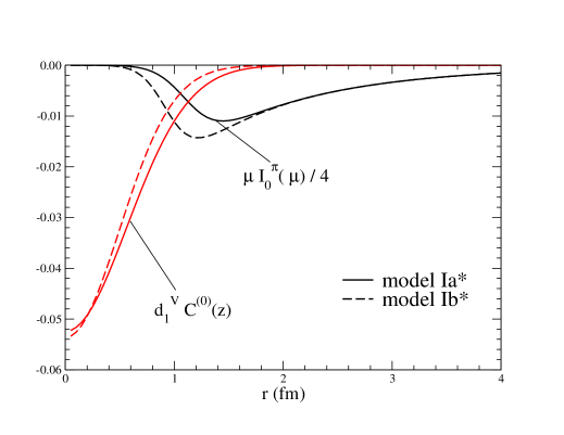
Figure 4: (Color online). Regularized correlation functions associated with the NLO and N3LO(NM) magnetic moment operators.

	$\mu(^{3}$He)		$\mu(^{3}$H)
	LO	N3LO	LO	N3LO
Ia	$-1.769$	$-2.119$	$2.585$	$2.969$
Ib	$-1.765$	$-2.122$	$2.579$	$2.970$
IIa	$-1.770$	$-2.126$	$2.588$	$2.973$
IIb	$-1.769$	$-2.131$	$2.586$	$2.981$

Table 5: The ³He and ³H magnetic moments in units of n.m., corresponding to the nuclear Hamiltonians Ia/b and IIa/b with current operators at LO and up to N3LO. The experimental values are $-2.126$ n.n. and $2.979$ n.m., respectively.

Finally, in Table 5 we report the ³He and ³H magnetic moments obtained with the Hamiltonians Ia/b and IIa/b Piarulli:2018 which differ from Ia^∗/b^∗ and IIa^∗/b^∗ only in the values adopted for the LECs $c_{D}$ and $c_{E}$ in the three-nucleon contact interaction. The results obtained with the three LECs in Table 1 (that is, without refitting $\mu_{d}$, $\mu_{S}$ and $\mu_{V}$) and by summing all corrections up to N3LO are well within less than a % of the experimental values, indicating that the wave functions of models a and b are close to those of models a^∗ and b^∗ (which reproduce these experimental values by design). As shown below, this conclusion remains valid also in the case of the magnetic form factors for momentum transfers $\lesssim 3$ fm^-1.

IV Predictions for selected electromagnetic observables

In this section we present predictions for the magnetic form factors of ²H, ³He, and ³H, deuteron photodisintegration at low energies (up to 30 MeV), and deuteron threshold electrodisintegration at backward angles up to four-momentum transfers $Q^{2}\lesssim 30$ fm^-2. (In this section, $Q$ denotes, rather than the generic low-momentum scale introduced earlier, the four-momentum transfer defined as $Q^{2}\,$=$\,q^{2}-\omega^{2}$, where $q$ and $\omega$ are the three-momentum and energy transfers, respectively.) There are extensive sets of experimental data on elastic electromagnetic cross sections and polarization observables of few-nucleon systems, and an up-to-date list of references to these can be found in the recent compilation by Marcucci et al. Marcucci:2016 . The experimental values for the form factors presented in the figures below result from fits to these data sets (the world data)—see Ref. Marcucci:2016 for a discussion of the procedure utilized to carry out the analysis. Experimental data on the deuteron low-energy photodisintegration and threshold electrodisintegration cross sections are from, respectively, Refs. Bishop:1950 ; Snell:1950 ; Colgate:1951 ; Carver:1951 ; Birenbaum:1985 ; Moreh:1989 ; DeGraeve:1992 and Rand:1967 ; Ganichot:1972 ; Simon:1979 ; Bernheim:1981 ; Auffret:1985 ; Schmitt:1997 (the deuteron electrodisintegration measurements at SLAC Arnold:1990 ; Frodyma:1993 are not considered here, since for these $Q^{2}\gtrsim 30$ fm^-2). The electrodisintegration data have been averaged over the interval 0–3 MeV of the recoiling $np$ center-of-mass energy (note that for the SLAC data this interval was 0–10 MeV).

Before comparisons with experimental data can be made, however, we need to include hadronic electromagnetic form factors in the current operators of Sec. II. These could be consistently calculated in chiral perturbation theory Kubis:2001 , but the convergence of these calculations in powers of the momentum transfer appears to be rather poor. For this reason, in the results reported below for the $A\,$= 2–3 form factors and deuteron electrodisintegration, they are taken from fits to available electron scattering data, as detailed in Ref. Piarulli:2013 ; specifically, in the LO and N2LO(RC) currents the replacements

$$\epsilon_{k}\longrightarrow\left[G_{E}^{S}(Q^{2})+G_{E}^{V}(Q^{2})\,\tau_{k,z}\right]\!/2\qquad{\rm and}\qquad\mu_{k}\longrightarrow\left[G_{M}^{S}(Q^{2})+G_{M}^{V}(Q^{2})\,\tau_{k,z}\right]\!/2\ ,$$ (31)

are made, where $G^{S/V}_{E}(Q^{2})$ and $G^{S/V}_{M}(Q^{2})$ denote the isoscalar/isovector combinations of the proton and neutron electric ($E$) and magnetic ($M$) form factors, normalized as $G^{S}_{E}(0)\,$=$\,G^{V}_{E}(0)$=$\,1$, $G^{S}_{M}(0)\,$=$\,\mu^{S}$, and $G^{V}_{M}(0)\,$=$\,\mu^{V}$ (we use the dipole parameterization Marcucci:2016 , including the Galster factor for the neutron electric form factor). The NLO and N3LO(LOOP) currents, and the isovector (isoscalar) terms of the N3LO(MIN) and N3LO(NM) currents, are multiplied by $G_{E}^{V}(Q^{2})$ [$G_{E}^{S}(Q^{2})$]. While for the NLO, N3LO(LOOP), and N3LO(MIN) currents a reasonable argument can be made based on current conservation for multiplying them by $G_{E}^{S}(Q^{2})$ and $G_{E}^{V}(Q^{2})$ Piarulli:2013 ; Marcucci:2016 , there is no a priori justification for the use of these nucleon form factors in the non-minimal contact current—they are simply included in order to provide a reasonable falloff of the interaction vertex with increasing $Q^{2}$. Lastly, the N2LO($\Delta$) current is multiplied by the $\gamma N\Delta$ electromagnetic form factor, taken from an analysis of $\gamma N$ data in the $\Delta$-resonance region Carlson:1986 and parametrized as

$$\frac{G_{\gamma N\Delta}(Q^{2})}{\mu_{\Delta N}}=\frac{1}{(1+Q^{2}/\Lambda_{\Delta,1}^{2})^{2}\sqrt{1+Q^{2}/\Lambda_{\Delta,2}^{2}}}\ ,$$ (32)

where $\mu_{\Delta N}$ is the nucleon-to-$\Delta$ transition magnetic moment introduced earlier, and cutoffs $\Lambda_{\Delta,1}\,$=$\,0.84$ GeV and $\Lambda_{\Delta,2}\,$=$\,1.2$ GeV, while the isoscalar N3LO(OPE) current, which in a resonance saturation picture reduces to the $\gamma\pi\rho$ current Pastore:2009 , is multiplied by a $\gamma\pi\rho$ transition form factor. By assuming vector-meson dominance, we parametrize it as

$$G_{\gamma\pi\rho}(Q^{2})=\frac{1}{1+Q^{2}/m_{\omega}^{2}}\ ,$$ (33)

where $m_{\omega}$ is the $\omega$-meson mass.

IV.1 Deuteron magnetic form factor

The magnetic form factor obtained with models Ia^∗/b^∗ and IIa^∗/b^∗ and currents at LO and by including corrections up to N3LO are compared to data in the left panel of Fig. 5. There is generally good agreement between theory and experiment for four-momentum transfer values $Q$ up to $\simeq\,$3 fm^-1. At higher $Q$’s, theory overestimates the data by a large factor, when the current retains the N3LO corrections; in particular, the diffraction seen in the data at $Q\,$$\simeq\,$ 7 fm^-1 is absent in the calculations. The cutoff dependence, as reflected by differences in the Ia^∗ and Ib^∗, IIa^∗ and IIb^∗ results, is negligible at the lower $Q$’s and moderate at the highest $Q$’s.

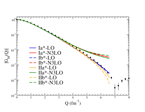
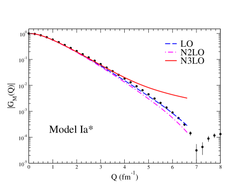
Figure 5: (Color online). Left panel: Predictions for the deuteron magnetic form factor, obtained with currents at LO and up to N3LO for models Ia^∗/b^∗ and IIa^∗/b^∗, are compared to the experimental data. Right panel: Cumulative contributions to the deuteron magnetic form factor, obtained at LO, N2LO, and N3LO for models Ia^∗, are compared to experimental data; note that the contributions at NLO, being isovector, vanish for this observable.

The cumulative contributions obtained with the LO, N2LO, and N3LO currents are illustrated for model I$a^{*}$ in the right panel of Fig. 5. Note that only the N2LO(RC), and N3LO(MIN), N3LO(NM), and N3LO(OPE) currents contribute to isoscalar observables. In particular, the N3LO(MIN) and N3LO(NM) ones have the same (isoscalar) operator structure and only differ in the LEC which multiplies it, either $m_{\pi}^{4}\,C_{5}/8$ for N3LO(MIN) or $d_{1}^{S}\,$=$\,m_{\pi}^{4}\,C_{15}^{\prime}$ for N3LO(NM). The combination $m_{\pi}^{4}\,C_{5}/8$ is Piarulli:2016 $\simeq$ –0.000195 (–0.000199) for model Ia^∗ (IIa^∗) and –0.000560 (–0.00108) for model Ib^∗ (IIb^∗), and should be compared to the values for $d_{1}^{S}$ reported in Table 1. Thus, the N3LO(MIN) contribution has the same sign as, but is suppressed by more than an order of magnitude relative to, the N3LO(NM) one. The N3LO(NM) and N3LO(OPE) contributions have the same (opposite) sign over the whole range of momentum transfers for models a^∗ (b^∗), see Fig. 6. The N3LO(NM) for models Ia^∗ and Ib^∗, and N3LO(OPE) for model Ia^∗, are the dominant contributions to the form factor in the high-$Q$ region. With the choice made for hadronic electromagnetic form factors noted above, it turns out that the momentum transfer falloff of the N3LO(NM) contribution is simply given by the isoscalar nucleon form factor $G_{E}^{S}(Q^{2})$, since the matrix element $\langle d|j^{\rm N3LO}_{{\rm NM},y}(q\hat{\bf x})|d\rangle/q$ is independent of $q$, see Eqs. (15) and (28). The sign and magnitude of the N3LO(OPE) contribution depend crucially on the interaction model—positive sign for models a and negative one for models b—for the reason explained in Sec. III.

Figure 6: (Color online). Magnitudes of individual contributions to the deuteron magnetic form factor (normalized to $\mu_{d}$ at $Q\,$=$\,0$) obtained with the N3LO(OPE) and N3LO(NM) currents for models Ia^∗ and Ib^∗. Note that the N3LO(MIN) contribution is not shown, since it is much smaller than the N3LO(NM) one (see text); also, to reduce clutter, since the LO and N2LO(RC) contributions for models Ia^∗ and Ib^∗ are very close to each other, they are only shown for model Ia^∗. The signs are as follows: positive for LO, N3LO(OPE)-Ia^∗, N3LO(NM) and negative for N2LO and N3LO(OPE)-Ib^∗ (for $Q\lesssim 6$ fm^-1).

It is interesting to compare the results obtained here for the deuteron magnetic form factor with those of Refs. Schiavilla:2002 and Piarulli:2013 . In Ref. Schiavilla:2002 a calculation of $G_{M}(Q)$ was carried out in the conventional meson-exchange picture based on the Argonne $v_{18}$ (AV18) interaction Wiringa:1995 . In Ref. Piarulli:2013 , instead, $G_{M}(Q)$ was studied both within a hybrid $\chi$EFT approach (i.e., based on the AV18 interaction and $\chi$EFT currents), and within a consistent $\chi$EFT approach, using the N3LO chiral interaction of Refs. Entem:2003 ; Machleidt:2011 (see also Ref. Marcucci:2016 ). In all theses cases, the complete calculation is unable to predict the magnetic form factor in the diffraction region $Q\simeq 7$ fm^-1, either underpredicting (in the case of the N3LO interaction) or overpredicting (in the case of the AV18 interaction, both within the conventional and hybrid approach) the experimental data.

IV.2 Trinucleon magnetic form factors

The magnetic form factors of ³He and ³H and their isoscalar and isovector combinations $F_{M}^{S}(Q)$ and $F_{M}^{V}(Q)$, normalized respectively as $\mu_{S}$ and $\mu_{V}$ at $Q\,$= 0, at LO for model Ia^∗, and with inclusion of corrections up to N3LO for all model interactions, are displayed in Fig. 7. As is well known from studies based on the conventional meson-exchange approach (see Ref. Carlson:1998 and references therein), two-body current contributions are crucial for filling in the zeros obtained in the LO calculation due to the interference between the S- and D-state components in the ground states of the trinucleons. For $Q\,$$\lesssim\,$2 fm^-1 there is excellent agreement between the present predictions and experimental data. However, as the momentum transfer increases, even after making allowance for the significant cutoff dependence (differences between a^∗ and b^∗ models), theory tends to underestimate the data; in particular, it predicts the zeros in the ³He and ³H magnetic form factors occurring at significantly lower values of $Q$ than observed. Inspection of the lower panels of Fig. 7 makes it clear that these discrepancies are primarily in the isovector form factor. Thus, the first diffraction region remains problematic for the present models, confirming results of calculations based both on meson-exchange phenomenology Carlson:1998 and earlier models of (momentum-space) chiral interactions Entem:2003 ; Machleidt:2011 and currents Piarulli:2013 .

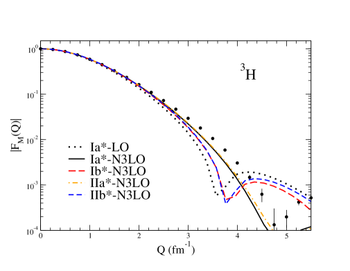
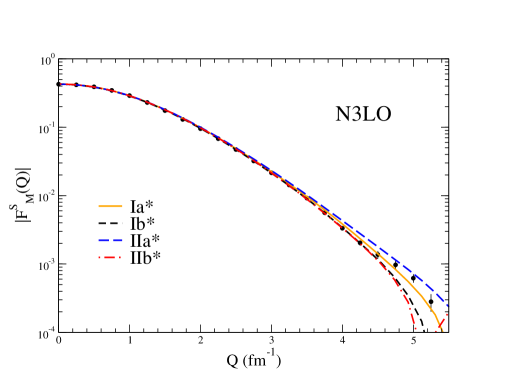
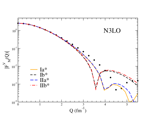
Figure 7: (Color online). Top panels: Predictions for the ³He and ³H magnetic form factors obtained with models Ia^∗/b^∗ and IIa^∗/b^∗ by including contributions up to N3LO in the current operator, are compared to data; also shown are the results for model Ia^∗ with the LO current operator. Bottom panels: Predictions for the isoscalar and isovector combinations of trinucleon magnetic form factors obtained with models Ia^∗/b^∗ and IIa^∗/b^∗ by including contributions up to N3LO in the current operator, are compared to data.

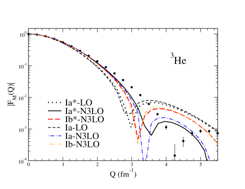
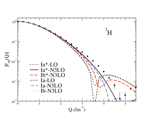
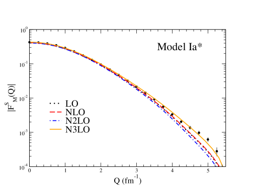
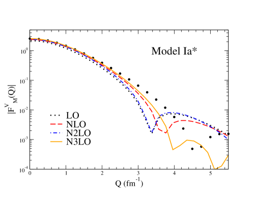
Figure 8: (Color online). Top panels: Predictions for the ³He and ³H magnetic form factors obtained with models Ia^∗/b^∗ and Ia/b by including contributions up to N3LO in the current operator, are compared to data; also shown are the results for models Ia^∗ and Ia with the LO current operator. Bottom panels: Cumulative contributions to the isoscalar and isovector combinations of trinucleon magnetic form factors, obtained at LO, NLO, N2LO, and N3LO for models Ia^∗, are compared to the experimental data.

The top panels of Fig. 8 illustrate the dependence of the LO and N3LO predictions on the three-nucleon interaction associated with the Hamiltonian models Ia/b and Ia^∗/b^∗. The variations are negligible at lower momentum transfer, and become perceptible only in the diffraction region of the form factors. The lower panels exhibit cumulatively the LO, NLO, N2LO, and N3LO contributions to the isoscalar and isovector form factors, obtained with model Ia^∗. Lastly, in Fig. 9 the contributions of the various terms in the current to these form factors are shown individually for models Ia^∗ and Ib^∗. The sign change of the N2LO($\Delta$) contribution at $Q\,$$\simeq\,$ 1.5 fm^-1 should be noted. As a consequence, while this contribution has the same sign as the NLO(OPE) and N3LO(NM) ones at low $Q$ ($\lesssim\,$ 1.5 fm^-1), it interferes destructively with them in the region $Q\,$$\simeq\,$ (3.0–3.4) fm^-1, where the LO form factor has a zero. This interference is largely responsible for the failure to reproduce the observed isovector form factor in the diffraction region.

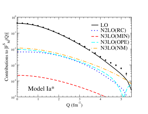
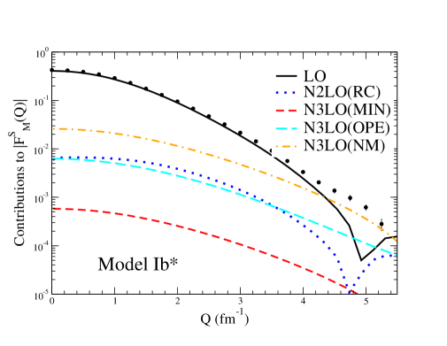
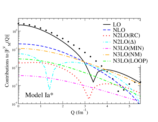
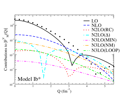
Figure 9: (Color online). Magnitudes of individual contributions to the isoscalar (top panels) and isovector (lower panels) form factors obtained for models Ia^∗ and Ib^∗. The signs for $F_{M}^{S}(Q)$ are as follows: positive for LO, N3LO(MIN), N3LO(OPE)-Ia^∗, N3LO(NM) and negative for N2LO and N3LO(OPE)-Ib^∗; the signs for $F_{M}^{V}(Q)$ are as follows: negative for LO, NLO, N2LO($\Delta$) (for $Q\,$$\lesssim\,$1.5 fm^-1), N3LO(NM), and N3LO(LOOP) and positive for N2LO(RC) and N3LO(MIN) for both models.

IV.3 Deuteron photodisintegration at low energies

At low energies, the photodisintegration process is dominated by the contributions of electric dipole ($E1$) and, to a much less but still significant extent, electric quadrupole ($E2$) transitions, connecting the deuteron to the $np$ ³P_J states with $J\,$=$\,0,1,2$ and ³S₁–³D₁ states, respectively (see, for example, Ref. Schiavilla:2005 ). As shown in the left panel of Fig. 10, the cross sections obtained with models Ia^∗/b^∗ and IIa^∗/b^∗ are weakly dependent on the set of cutoff radii $(R_{\rm S},R_{\rm L})$ regularizing the two-nucleon interactions and currents, and are systematically lower than the experimental data.

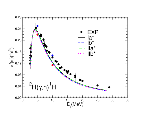
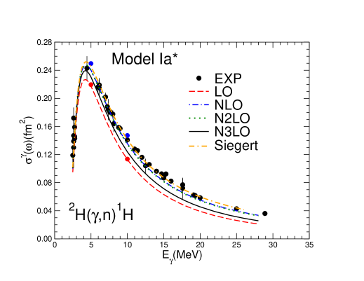
Figure 10: Left panel: The low-energy deuteron photodisintegration data (black, blue, and red filled circles) are compared to predictions obtained with models Ia^∗, Ib^∗, IIa^∗, and IIb^∗, including terms up to N3LO in the current operator. Right panel: Cumulative contributions to the low-energy deuteron photodisintegration cross section, obtained at LO, NLO, N2LO, and N3LO for models Ia^∗, are compared to experimental data; also shown are the results obtained with the Siegert form of the $E1$ transition operator.

In the right panel of Fig. 10, the cumulative contributions at LO, NLO, N2LO, and N3LO are displayed for model Ia^∗. The N2LO corrections to this observable are found to be negligible (the NLO and N2LO curves lay almost on top of each other). This is because the $\Delta$-excitation current—the leading among the terms at N2LO—has magnetic dipole character, and therefore primarily contributes to magnetic dipole ($M1$) transitions, whose strength is much suppressed relative to $E1$ in the energy regime of interest here. Of course, $M1$ transitions become important at threshold and a few-hundred keV’s above threshold; at higher energy, they play a role in polarization observables, as in $P^{\prime}_{y}$—the neutron induced polarization—which in fact results from interference of $E1$ and $M1$ transitions Schiavilla:2005 (unfortunately, experimental data on this observable in the few MeV range have large uncertainties, and for this reason $P^{\prime}_{y}$ has not been studied in the present work).

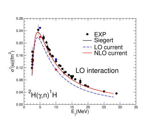
Figure 11: The low-energy deuteron photodisintegration cross section, obtained with the LO interaction of Ref. Piarulli:2016 and currents at LO and up to NLO; also shown are the results obtained with the Siegert form of the $E1$ transition operator: the curves labeled “Siegert” and “NLO current” overlap. The data are represented by the (black, blue, and red) filled circles.

Of course, $E1$ strength can also be calculated by making use of the Siegert form for the associated transition operator. Because of the way the calculations are carried out in practice (see Ref. Schiavilla:2005 for a summary of the methods), this is most easily implemented by exploiting the identity Schiavilla:2004

$${\bf j}({\bf q})={\bf j}({\bf q})-{\bf j}({\bf q}=0)+i\,\left[H\,,\,\int d{\bf x}\,{\bf x}\,\rho({\bf x})\right]\ ,$$ (34)

where $H$ is the nuclear Hamiltonian and $\rho({\bf x})=\delta({\bf x}-{\bf r}_{i})\,\epsilon_{i}+\delta({\bf x}-{\bf r}_{j})\,\epsilon_{j}$ is the charge density operator ($\epsilon_{i}$ is the proton projection operator introduced earlier). Hence, in evaluating matrix elements between the initial deuteron state and final $np$ scattering state, the commutator term simply reduces to

$$i\,\left[H\,,\,\int d{\bf x}\,{\bf x}\,\rho({\bf x})\right]\longrightarrow i\,q\,\sum_{i}\epsilon_{i}\,{\bf r}_{i}\ ,$$ (35)

where $q$ is the photon energy. It should be emphasized that the identity above assumes that the current ${\bf j}({\bf q})$ is conserved. The results of the calculation based on the r.h.s. of Eq. (34) are shown in the right panel of Fig. 10 (curve labeled Siegert): they are in agreement with data, thus suggesting that the discrepancies seen at N3LO arise because of the lack of current conservation.

In order to corroborate this interpretation, we have carried out a calculation using the interaction at LO (OPE plus LO contact terms proportional to $C_{S}$ and $C_{T}$) fitted to the deuteron binding energy and two-nucleon scattering data up to energies of 125 MeV, first row of Table I in Ref. Piarulli:2016 . With this interaction, the current including the LO and NLO terms of Eqs. (1) and (3) is exactly conserved in the low $q$ limit. Indeed at $q\,$= 0, specifically for the NLO current we have

$${\bf j}^{\rm NLO}(0)=-\frac{g_{A}^{2}}{48\,\pi}\,\frac{m^{2}_{\pi}}{f_{\pi}^{2}}\left({\bm{\tau}}_{i}\times{\bm{\tau}}_{j}\right)_{z}\,\hat{\bf r}_{ij}\,\,C_{R_{\rm L}}(r)\,\,{\rm e}^{-\mu}\left[\left(\frac{3}{\mu^{2}}+\frac{3}{\mu}+1\right)S_{ij}+{\bm{\sigma}}_{i}\cdot{\bm{\sigma}}_{j}\right]\ ,$$ (36)

and up to linear terms in the momentum transfer ${\bf q}\cdot{\bf j}^{\rm NLO}(0)=\left[v^{\rm LO}_{ij}\,,\,\rho({\bf q})\right]$, where $v^{\rm LO}_{ij}$ and $\rho({\bf q})={\rm e}^{i{\bf q}\cdot{\bf r}_{i}}\,\epsilon_{i}+{\rm e}^{i{\bf q}\cdot{\bf r}_{j}}\,\epsilon_{j}$ are, respectively, the LO interaction and Fourier transform of the LO charge operator introduced above. The results of this calculation are displayed in Fig. 11. As expected, the curves labeled “NLO current” and “Siegert” overlap each other.

Strict adherence to current conservation in the presence of N3LO corrections to the interaction requires going up to N5LO in the derivation of the electromagnetic operators Marcucci:2016 , a rather daunting task (even in a $\chi$EFT framework with nucleons and pions only, that ignores $\Delta$ isobars). It is also unclear how many new LECs would enter, in addition to the current three, at that order; if there were to be too many, this would obviously reduce substantially the predictive power of the theory, since there is only a limited number of electromagnetic observables in the few-nucleon systems (including single nucleons) to constrain these LECs.

IV.4 Deuteron threshold electrodisintegration at backward angles

The dominant component of the cross section for deuteron electrodisintegration near threshold at backward angles is the $M1$ transition between the bound deuteron and the ¹S₀ scattering state Hockert:1973 . As is well known, at large values of $Q$ this transition rate is dominated by two-body current contributions. The corrections from higher partial waves in the final $np$ scattering state are significantly smaller. Here we take into account all partial waves in the final state, with full account of the strong interaction in relatives waves with $J\leq 5$ ($J$ is the total angular momentum) Schiavilla:1991 . Final-state interaction effects in higher partial waves have been found to be numerically negligible.

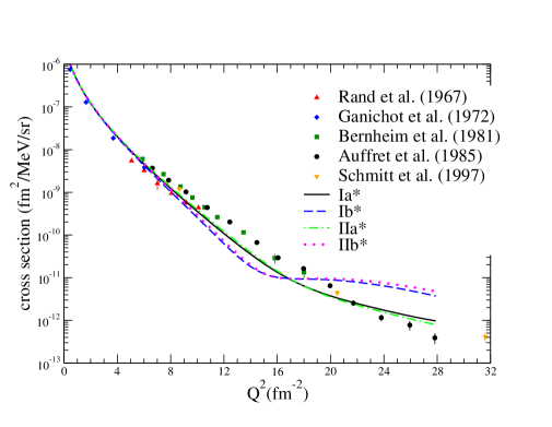
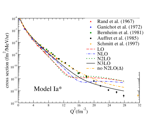
Figure 12: Left panel: The deuteron threshold electrodisintegration data at backward angles are compared to predictions obtained with interaction models Ia^∗, Ib^∗, IIa^∗, and IIb^∗, including terms up to N3LO in the current operator. Right panel: Cumulative contributions obtained with currents at LO, NLO, N2LO, and N3LO for model Ia^∗; also shown are the results at N3LO but excluding the N2LO($\Delta$) current.

In Fig. 12 we compare the calculated cross sections for backward electrodisintegration with the experimental values. While the data have been averaged over the interval 0–3 MeV of the final $np$-pair center-of-mass energy, the theoretical results have been computed at a fixed energy of 1.5 MeV. It is known that the effect of the width of the energy interval over which the cross section values are averaged is very small Schiavilla:1991 . The data, while well reproduced at low values of $Q^{2}$, are at variance with theory as $Q^{2}$ increases beyond 10 fm^-2, particularly for the set of harder cutoffs $(R_{\rm S},R_{\rm L})=(0.7,1.0)$ fm of the b models of interactions and currents. There is a large cutoff dependence (left panel of Fig. 12) for $Q\,$$\gtrsim\,$10 fm^-2, perhaps not surprisingly given that the largest four-momentum transfers are comparable, and in fact exceed, the hard scale $\Lambda_{\chi}$, below which the $\chi$EFT framework is well defined. Nevertheless, it is interesting to note that the trend seen in the present calculations, even at these high $Q^{2}$’s, is quantitatively similar to that obtained with interactions and currents derived from meson-exchange phenomenology, see Refs. Carlson:1998 ; Schiavilla:1991 .

Cumulative contributions at LO, NLO, N2LO, and N3LO are illustrated for model Ia^∗ in the right panel of Fig. 12. The sharp zero in the LO results seen when only the ¹S₀ $np$ final state is included Schiavilla:1991 , resulting from destructive interference between the transitions to this state from the S- and D-wave components of the deuteron, is filled in by the contributions of higher partial waves. As in the case of the trinucleon isovector magnetic form factor, for $Q^{2}\,$$\gtrsim\,$2 fm^-2 the signs of the contributions of the currents at LO and NLO, and at N2LO($\Delta$), are opposite, and the resulting cancellation significantly worsens the agreement between theory and experiment, see curve labeled “no N2LO($\Delta$)” in the right panel of Fig. 12.

V Conclusions

We have carried out a study of magnetic structure and response of the deuteron and trinucleons with chiral interactions and electromagnetic currents including $\Delta$ intermediate states. These interactions and currents have been derived and regularized in configuration space. While $\Delta$ contributions from leading and sub-leading $\pi N\Delta$ couplings are accounted for in the TPE component of the two-nucleon interaction Piarulli:2015 , only those at tree level from leading $\gamma N\Delta$ and $\pi N\Delta$ couplings are retained in the OPE and TPE components of, respectively, the two-body current and three-nucleon interaction Piarulli:2018 . The predicted magnetic form factors of deuteron and trinucleons are in excellent agreement with experimental data for momentum transfers corresponding to 3–4 pion masses, and exhibit a rather weak cutoff dependence in this range, as reflected by the differences between interaction models a and b. The present results confirm those of earlier studies Piarulli:2013 , based on chiral interactions Entem:2003 ; Machleidt:2011 and currents formulated in momentum space, and which did not include explicitly $\Delta$ degrees of freedom, albeit the cutoff variation here appears to be significantly reduced when compared to that seen in Ref. Piarulli:2013 , particularly at larger values of momentum transfers. In this higher momentum-transfer region, the calculations overestimate the observed deuteron magnetic form factor by an order of magnitude, and in particular do not reproduce the zero seen in the data at $Q\,$$\simeq$ 7 fm^-1. In this region the dominant contributions are from the non-minimal contact current and, in the case of the a models, the isoscalar OPE current. These currents are proportional to the LECs $d_{1}^{S}$ and $d_{2}^{S}$ which have been fixed by properties at vanishing momentum transfer (the magnetic moments $\mu_{d}$ and $\mu^{S}$), and include hadronic electromagnetic form factors, which we have taken, respectively, as $G_{E}^{S}(Q^{2})$—arbitrarily—and as $G_{\gamma\pi\rho}(Q^{2})$ by assuming vector dominance. So for these reasons, predictions at the higher $Q^{2}$ should be viewed as rather uncertain, even after setting aside justified concerns one might have about the validity of the present $\chi$EFT framework in a regime where the momentum transfer exceeds the hard scale $\Lambda_{\chi}\,$$\simeq\,$1 GeV.

The zeros in the magnetic form factors of ³He and ³H are shifted to lower momentum transfer than observed. Thus, the description of the experimental data at these larger momentum transfers remains problematic, a difficulty already exhibited by previous $\chi$EFT calculations Piarulli:2013 as well as by older calculations based on meson-exchange phenomenology Marcucci:1998 . This discrepancy is primarily in the isovector combination of the trinucleon form factors, and is likely to have its origin in a somewhat too weak overall strength of the isovector component of the electromagnetic current at large momentum transfer. By contrast, the calculated isoscalar combination is very close to data over the whole range of momentum transfers considered. It is interesting to note in this connection that the N2LO($\Delta$) contribution associated with the (isovector) $\Delta$-excitation current is comparable in magnitude to, and of opposite sign than, the NLO contribution in the diffraction region, see lower right panel of Fig. 9. This destructive interference then appears to be the culprit of the current failure of theory to reproduce experiment. Similar considerations also apply to the deuteron threshold electrodisintegration cross sections at backward angles, which are underestimated by theory for $Q^{2}\,$$\gtrsim\,$8 fm^-2—a failure known to occur in the older meson-exchange calculations too (see Ref. Carlson:1998 and references therein).

The sign change of the contribution associated with the $\Delta$-excitation current also occurred in the Marcucci et al. calculations of trinucleon form factors Marcucci:1998 , albeit at a larger momentum transfer than here ($Q\,$$\simeq\,$3 fm^-1 versus $\simeq\,$ 1.5 fm^-1), presumably due to the much harder cutoff adopted in that work. In the Marcucci et al. paper, contributions which in a $\chi$EFT approach would approximately correspond to TPE terms with $\Delta$ intermediate states in two- and three-body currents, were also considered, and found to have the same sign as, but to be suppressed by an order of magnitude relative to, those from the OPE current. Whether this estimate of $\Delta$ effects at the TPE level remains valid in the present $\chi$EFT framework is an open question we hope to address in the future.

Finally, we have shown that the inability of theory to provide a satisfactory description of the measured deuteron photodisintegration cross sections at low energies originates from the lack of current conservation. This flaw can be corrected, at least in processes in which electric-dipole transitions are dominant, by making use of the Siegert form of the $E1$ operator. In practical calculations this is most easily implemented via the replacements in the r.h.s. of Eqs. (34)–(35).

We conclude by noting that the present work complements that of Ref. Baroni:2018 . Together, these two papers provide the complete set of chiral electroweak currents at one loop with fully constrained LECs for use with the local chiral interactions developed in Ref. Piarulli:2016 (models Ia/b and IIa/b) and Ref. Baroni:2018 (models Ia^∗/b^∗ and IIa^∗/b^∗), thus opening up the possibility to study radiative and weak transitions in systems with mass number $A>4$ with QMC methods, and low-energy neutron and proton radiative captures on deuteron and ³H/³He, and proton weak capture on ³He (the Hep process) with HH techniques. Work along these lines is in progress.

One of the authors (R.S.) thanks the T-2 group in the Theoretical Division at LANL, and especially J. Carlson and S. Gandolfi, for the support and warm hospitality extended to him during a sabbatical visit in the Fall 2018, when part of this research was completed. The support of the U.S. Department of Energy, Office of Science, Office of Nuclear Physics, under contracts DE-AC05-06OR23177 (R.S.) and DE-AC02-06CH11357 (A.L., M.P., S.C.P., and R.B.W.), and award DE-SC0010300 (A.B.), is gratefully acknowledged. The work of A.L., S.P., M.P., S.C.P., and R.B.W. has been further supported by the NUclear Computational Low-Energy Initiative (NUCLEI) SciDAC project. Computational resources provided by the National Energy Research Scientific Computing Center (NERSC) are also thankfully acknowledged.

Appendix A Loop corrections to the electromagnetic current in configuration space

In this appendix we sketch the derivation of the configuration-space expressions for the loop corrections to the electromagnetic current. At low momentum transfer (denoted as q), these corrections read in momentum space Pastore:2009 ; Piarulli:2013

$${\widetilde{\bf j}}^{\,{\rm N3LO}}_{\,\rm TPE}({\bf k}_{ij})=i\,\tau_{j,z}\left[\widetilde{F}_{0}(k_{ij})\,{\bm{\sigma}}_{i}-\widetilde{F}_{2}(k_{ij})\,\frac{{\bf k}_{ij}\,{\bm{\sigma}}_{i}\cdot{\bf k}_{ij}}{k_{ij}^{2}}\right]\times\frac{{\bf q}}{2\,m_{\pi}}-i\,({\bm{\tau}}_{i}\times{\bm{\tau}}_{j})_{z}\,{\bm{\nabla}}_{{\!k}_{ij}}\,\widetilde{F}_{1}(k_{ij})+(i\rightleftharpoons j)\ ,$$ (37)

where we have defined

$${\bf k}_{ij}=({\bf k}_{i}-{\bf k}_{j})/2\ ,\qquad{\bf q}={\bf k}_{i}+{\bf k}_{j}\ ,$$ (38)

and

$$\widetilde{F}_{0}(k) = \frac{g_{A}^{2}}{128\,\pi^{2}}\,\frac{2\,m_{\pi}}{f_{\pi}^{4}}\,\left\{1-2\,g_{A}^{2}+\frac{8\,g_{A}^{2}\,m_{\pi}^{2}}{k^{2}+4\,m_{\pi}^{2}}+G(k)\left[2-2\,g_{A}^{2}-\frac{4\,(1+g_{A}^{2})\,m_{\pi}^{2}}{k^{2}+4\,m_{\pi}^{2}}+\frac{16\,g_{A}^{2}\,m_{\pi}^{4}}{(k^{2}+4\,m_{\pi}^{2})^{2}}\right]\right\}\ ,$$ (39)

$$\widetilde{F}_{1}(k) = \frac{1}{1536\,\pi^{2}\,f_{\pi}^{4}}\,G(k)\bigg{[}4m_{\pi}^{2}(1+4g_{A}^{2}-5g_{A}^{4})+k^{2}(1+10g_{A}^{2}-23g_{A}^{4})-\frac{48\,g_{A}^{4}m^{4}_{\pi}}{4\,m^{2}_{\pi}+k^{2}}\bigg{]}\ ,$$ (40)

$$\widetilde{F}_{2}(k) = \frac{g_{A}^{2}}{128\,\pi^{2}}\,\frac{2\,m_{\pi}}{f_{\pi}^{4}}\,\left\{2-6\,g_{A}^{2}+\frac{8\,g_{A}^{2}\,m_{\pi}^{2}}{k^{2}+4\,m_{\pi}^{2}}+G(k)\left[4\,g_{A}^{2}-\frac{4\,(1+3\,g_{A}^{2})\,m_{\pi}^{2}}{k^{2}+4\,m_{\pi}^{2}}+\frac{16\,g_{A}^{2}\,m_{\pi}^{4}}{(k^{2}+4\,m_{\pi}^{2})^{2}}\right]\right\}\ ,$$ (41)

with the loop function $G(k)$ given by

$$G(k)=\frac{\sqrt{4\,m_{\pi}^{2}+k^{2}}}{k}\ln\frac{\sqrt{4\,m_{\pi}^{2}+k^{2}}+k}{\sqrt{4\,m_{\pi}^{2}+k^{2}}-k}\ .$$ (42)

We note that the term $\widetilde{F}_{1}(k)$ is related to the TPE interaction ${\bm{\tau}}_{i}\cdot{\bm{\tau}}_{j}\,\widetilde{v}^{\,{\rm NLO}}_{\,2\pi}(k)$ (in a $\chi$EFT with nucleon and pion degrees of freedom only) via $\widetilde{F}_{1}(k)=\widetilde{v}^{\,{\rm NLO}}_{\,2\pi}(k)/2$, and that the longitudinal term proportional to $\widetilde{F}_{1}(k)$ satisfies current conservation with this interaction (in the limit of small $q$), namely

$$\left[\,\widetilde{v}^{\,{\rm NLO}}_{\,2\pi}(|{\bf k}_{ij}-{\bf q}/2|)\,{\bm{\tau}}_{i}\cdot{\bm{\tau}}_{j}\,\,,\,\,\frac{1+\tau_{i,z}}{2}\,\right]+(i\rightleftharpoons j)=-i\,({\bm{\tau}}_{i}\times{\bm{\tau}}_{j})_{z}\,{\bf q}\cdot{\bm{\nabla}}_{{\bf k}_{ij}}\,\widetilde{F}_{1}(k_{ij})+(i\rightleftharpoons j)\ .$$ (43)

In configuration space, we obtain

$${\bf j}^{\,{\rm N3LO}}_{\,\rm TPE}({\bf q}) = i\,\tau_{j,z}\,\,{\rm e}^{i{\bf q}\cdot{\bf R}_{ij}}\left[{\bm{\sigma}}_{i}\int_{\bf k}{\rm e}^{i{\bf k}\cdot{\bf r}_{ij}}\widetilde{F}_{0}(k)+\left(2\,m_{\pi}\right)^{2}\left({\bm{\sigma}}_{i}\cdot{\bm{\nabla}}^{{\lambda}_{ij}}\right)\,{\bm{\nabla}}^{{\lambda}_{ij}}\int_{\bf k}{\rm e}^{i{\bf k}\cdot{\bf r}_{ij}}\,\,\frac{\widetilde{F}_{2}(k)}{k^{2}}\,\right]\times\frac{{\bf q}}{2\,m_{\pi}}$$ (44)

$$-\frac{1}{2}({\bm{\tau}}_{i}\times{\bm{\tau}}_{j})_{z}\,\,{\rm e}^{i{\bf q}\cdot{\bf R}_{ij}}\,{\bf r}_{ij}\,v_{\,2\pi}^{\rm NLO}(r_{ij})+(i\rightleftharpoons j)\ ,$$

where ${\bm{\nabla}}^{{\lambda}_{ij}}={\partial}/{\partial{\bm{\lambda}}_{ij}}$ (${\bm{\lambda}}_{ij}\,$=$\,2\,m_{\pi}\,{\bf r}_{ij}$) and $\int_{\bf k}=\int\!{d{\bf k}}/{(2\pi)^{3}}$. The Fourier transforms of $\widetilde{F}_{0}(k)$ and $\widetilde{F}_{2}(k)/k^{2}$ in terms of $x=k/\left(2\,m_{\pi}\right)$ reduce to (dropping the subscripts $ij$)

$$\int_{\bf k}{\rm e}^{i{\bf k}\cdot{\bf r}}\,\widetilde{F}_{0}(k) = \frac{(2\,m_{\pi})^{3}}{2\,\pi^{2}}\,\frac{1}{\lambda}\int_{0}^{\infty}dx\,x\,{\rm sin}(x\lambda)\,\widetilde{F}_{0}(x)\ ,$$ (45)

$$\left(2\,m_{\pi}\right)^{2}\int_{\bf k}{\rm e}^{i{\bf k}\cdot{\bf r}}\,\frac{\widetilde{F}_{2}(k)}{k^{2}} = \frac{\left(2\,m_{\pi}\right)^{3}}{2\,\pi^{2}}\,\frac{1}{\lambda}\int_{0}^{\infty}dx\,\frac{{\rm sin}(x\lambda)}{x}\,\widetilde{F}_{2}(x)\ .$$ (46)

In order to carry out the sine transforms above, we find it convenient to express $G(x)$ in Eq. (42) as

$$G(x)=2+G^{\star}(x)\ ,\qquad G^{\star}(x)=\int_{0}^{1}dz\,{\rm ln}\left[1+x^{2}\left(1-z^{2}\right)\right]\ ,$$ (47)

and $G^{\star}(x)$ diverges logarithmically in the limit $|x|\gg 1$. In terms of the variable $x$, the functions $F_{i}(x)$ are written as

$$\frac{\left(2\,m_{\pi}\right)^{3}}{2\,\pi^{2}}\widetilde{F}_{i}(x)=A_{i}(x)+G^{\star}(x)\,B_{i}(x)\ ,$$ (48)

where

$$A_{0}(x) = \frac{g_{A}^{2}}{256\,\pi^{4}}\,\frac{\left(2\,m_{\pi}\right)^{4}}{f_{\pi}^{4}}\left[5-6\,g_{A}^{2}-\frac{2}{x^{2}+1}+\frac{2\,g_{A}^{2}}{\left(x^{2}+1\right)^{2}}\right]\ ,$$ (49)

$$B_{0}(x) = \frac{g_{A}^{2}}{256\,\pi^{4}}\,\frac{\left(2\,m_{\pi}\right)^{4}}{f_{\pi}^{4}}\left[2-2\,g_{A}^{2}-\frac{1+g_{A}^{2}}{x^{2}+1}+\frac{g_{A}^{2}}{\left(x^{2}+1\right)^{2}}\right]\ ,$$ (50)

$$A_{2}(x) = \frac{g_{A}^{2}}{128\,\pi^{4}}\,\frac{\left(2\,m_{\pi}\right)^{4}}{f_{\pi}^{4}}\left[1+g_{A}^{2}-\frac{1+2\,g_{A}^{2}}{x^{2}+1}+\frac{g_{A}^{2}}{\left(x^{2}+1\right)^{2}}\right]\ ,$$ (51)

$$B_{2}(x) = \frac{g_{A}^{2}}{256\,\pi^{4}}\,\frac{\left(2\,m_{\pi}\right)^{4}}{f_{\pi}^{4}}\left[4\,g_{A}^{2}-\frac{1+3\,g_{A}^{2}}{x^{2}+1}+\frac{g_{A}^{2}}{\left(x^{2}+1\right)^{2}}\right]\ .$$ (52)

We then obtain

$$\int_{\bf k}{\rm e}^{i{\bf k}\cdot{\bf r}}\,\widetilde{F}_{0}(k) = \frac{1}{2\,\lambda}\int_{-\infty}^{\infty}dx\,x\,{\rm sin}(x\lambda)\left[A_{0}(x)+G^{\star}(x)\,B_{0}(x)\right]\ ,$$ (53)

$$\left(2\,m_{\pi}\right)^{2}\int_{\bf k}{\rm e}^{i{\bf k}\cdot{\bf r}}\,\,\frac{\widetilde{F}_{2}(k)}{k^{2}} = \,\frac{1}{2\,\lambda}\int_{-\infty}^{\infty}dx\,\frac{{\rm sin}(x\lambda)}{x}\left[A_{2}(x)+G^{\star}(x)\,B_{2}(x)\right]\ ,$$ (54)

where the integration limits over $x$ have been extended to the range $(-\infty,\infty)$. The function $F_{0}(x)$ diverges in the limit $x\longrightarrow\infty$ and must be regularized before the sine transform can be carried out. To this end, we define

$$A_{0}^{\infty}(x) = \frac{g_{A}^{2}}{256\,\pi^{4}}\,\frac{\left(2\,m_{\pi}\right)^{4}}{f_{\pi}^{4}}\left(5-6\,g_{A}^{2}\right)\ ,$$ (55)

$$B^{\infty}_{0}(x) = \frac{g_{A}^{2}}{256\,\pi^{4}}\,\frac{\left(2\,m_{\pi}\right)^{4}}{f_{\pi}^{4}}\left(2-2\,g_{A}^{2}\right)\ ,$$ (56)

and then choose to subtract from $F_{0}(x)$ its asymptotic behavior proportional to $A^{\infty}_{0}(x)+G^{\star}(x)B_{0}^{\infty}(x)$, namely

$$\frac{\left(2\,m_{\pi}\right)^{3}}{2\,\pi^{2}}\overline{F}_{0}(x) = \frac{\left(2\,m_{\pi}\right)^{3}}{2\,\pi^{2}}\left[\widetilde{F}_{0}(x)-F_{0}^{\infty}(x)\right]=\overline{A}_{0}(x)+G^{\star}(x)\,\overline{B}_{0}(x)\ ,$$ (57)

where

$$\overline{A}_{0}(x) = -\frac{g_{A}^{2}}{128\,\pi^{4}}\,\frac{\left(2\,m_{\pi}\right)^{4}}{f_{\pi}^{4}}\frac{1}{x^{2}+1}\left(1-\frac{g_{A}^{2}}{x^{2}+1}\right)\ ,$$ (58)

$$\overline{B}_{0}(x) = -\frac{g_{A}^{2}}{256\,\pi^{4}}\,\frac{\left(2\,m_{\pi}\right)^{4}}{f_{\pi}^{4}}\frac{1}{x^{2}+1}\left(1+g_{A}^{2}-\frac{g_{A}^{2}}{x^{2}+1}\right)\ .$$ (59)

The Fourier transform of $F_{0}^{\infty}(k)$ is then regularized by multiplication of a Gaussian cutoff ${\rm exp}\left(-k^{2}R^{2}_{\rm S}/4\right)$ as in Eq. (18) to obtain ($z\,$=$\,r/R_{\rm S}$)

$$F^{(0)}(z;\infty) = \frac{g_{A}^{4}}{1024\,\pi^{2}}\,\frac{\left(2\,m_{\pi}\right)^{4}}{f_{\pi}^{4}}\left(\frac{1}{g_{A}^{2}}-2\right)C^{(0)}_{R_{\rm S}}(z)$$ (60)

$$+\frac{g_{A}^{4}}{1024\,\pi^{4}}\,\frac{\left(2\,m_{\pi}\right)^{4}}{f_{\pi}^{4}}\frac{1}{\left(m_{\pi}R_{\rm S}\right)^{3}}\left(\frac{1}{g_{A}^{2}}-1\right)\int_{0}^{\infty}\!\ dx\,x^{2}\,j_{0}(xz)\,G(x/R_{\rm S})\,{\rm e}^{-x^{2}/4}\ ,$$

where we have reinstated the function $G(k)$ in the second line of the above equation.

A.1 Sine transforms

We collect here the formulae needed for the sine transforms involving $G^{\star}(x)$ (those without $G^{\star}(x)$ are elementary)

$$\int_{-\infty}^{\infty}dx\,x\,{\rm sin}(x\lambda)\,\frac{G^{\star}(x)}{x^{2}+1}=\pi\!\!\int_{0}^{1}dz\,\Big{[}{\rm e}^{-\lambda}\,E_{1}\left(\lambda\,\alpha_{z}-\lambda\right)+{\rm e}^{\lambda}\,E_{1}\left(\lambda\,\alpha_{z}+\lambda\right)\Big{]}-2\,\pi\,{\rm e}^{-\lambda}\ ,$$ (64)

$$\int_{-\infty}^{\infty}dx\,x\,{\rm sin}(x\lambda)\,\frac{G^{\star}(x)}{(x^{2}+1)^{2}}=-\pi\,\lambda\,{\rm e}^{-\lambda}+\pi\,{\rm e}^{-\lambda}\int_{0}^{1}dz\,\frac{1}{\alpha_{z}^{2}-1}\left[1-{\rm e}^{-\lambda(\alpha_{z}-1)}\right]$$

$$\hskip 14.22636pt+\frac{\pi}{2}\int_{0}^{1}dz\Big{[}\lambda\,{\rm e}^{-\lambda}\,E_{1}\left(\lambda\,\alpha_{z}-\lambda\right)-\lambda\,{\rm e}^{\lambda}\,E_{1}\left(\lambda\,\alpha_{z}+\lambda\right)\Big{]}\ ,$$

$$\int_{-\infty}^{\infty}dx\,\frac{{\rm sin}(x\lambda)}{x}\,G^{\star}(x)=2\,\pi\int_{0}^{1}dz\,E_{1}(\lambda\,\alpha_{z})\ ,$$

$$\int_{-\infty}^{\infty}dx\,\frac{{\rm sin}(x\lambda)}{x}\,\frac{G^{\star}(x)}{x^{2}+1}=2\,\pi\left[{\rm e}^{-\lambda}+\int_{0}^{1}dz\,E_{1}\left(\lambda\,\alpha_{z}\right)\right]-\,\pi\int_{0}^{1}dz\,\Big{[}{\rm e}^{-\lambda}\,E_{1}\left(\lambda\,\alpha_{z}-\lambda\right)+{\rm e}^{\lambda}\,E_{1}\left(\lambda\,\alpha_{z}+\lambda\right)\Big{]}\ ,$$

$$\int_{-\infty}^{\infty}dx\,\frac{{\rm sin}(x\lambda)}{x}\,\frac{G^{\star}(x)}{(x^{2}+1)^{2}} = 2\,\pi\left(1+\frac{\lambda}{2}\right){\rm e}^{-\lambda}-\pi\,{\rm e}^{-\lambda}\int_{0}^{1}dz\,\frac{1}{\alpha_{z}^{2}-1}\left[1-{\rm e}^{-\lambda(\alpha_{z}-1)}\right]$$ (65)

$$-\pi\int_{0}^{1}dz\left[\left(1+\frac{\lambda}{2}\right){\rm e}^{-\lambda}\,E_{1}\left(\lambda\,\alpha_{z}-\lambda\right)+\left(1-\frac{\lambda}{2}\right){\rm e}^{\lambda}\,E_{1}\left(\lambda\,\alpha_{z}+\lambda\right)-2\,E_{1}\left(\lambda\,\alpha_{z}\right)\right]\ ,$$

where

$$\alpha_{z}=\frac{1}{\sqrt{1-z^{2}}}\geq 1\ ,$$ (66)

and we have introduced the exponential integral defined as Abramowitz:1972

$$E_{1}(x)=\int_{x}^{\infty}dt\,\frac{{\rm e}^{-t}}{t}\ ,$$ (67)

with the following series expansion and asymptotic behavior

$$E_{1}(x)=-\gamma-{\rm ln}\,x-\sum_{n=1}^{\infty}(-1)^{n}\,\frac{x^{n}}{n\,n!}\ ,\qquad E_{1}(x)=\frac{{\rm e}^{-x}}{x}\left(1-\frac{1!}{x}+\frac{2!}{x^{2}}-\frac{3!}{x^{3}}+\cdots\right)\,\,\,{\rm for}\,\,\,x\gg 1\ ,$$ (68)

and $\gamma$ is Euler’s number.

We will now illustrate the evaluation of one of the integrals above, which we carry out by contour integration in the complex plane by proceeding in a similar way as in Ref. Baroni:2018 . We consider

$$\!\!\!\!\!\!\!\int_{-\infty}^{\infty}dx\,x\,{\rm sin}(x\lambda)\,\frac{G^{\star}(x)}{x^{2}+a^{2}} = \!\int_{0}^{1}dz\,\,{\rm Im}\int_{-\infty}^{\infty}dx\,\frac{x}{x^{2}+a^{2}}\,{\rm e}^{i\,x\lambda}\,{\rm ln}\left[1+x^{2}\left(1-z^{2}\right)\right]$$ (69)

$$= \!\left[\int_{0}^{1}dz\,{\rm ln}\left(1-z^{2}\right)\right]{\rm Im}\int_{-\infty}^{\infty}dx\,\frac{x}{x^{2}+a^{2}}\,{\rm e}^{i\,x\lambda}+\int_{0}^{1}dz\,I(z,\lambda),$$

where $a$ is a parameter ($a=1$ is the value of interest) and

$$I(z,\lambda)={\rm Im}\int_{-\infty}^{\infty}dx\,\frac{x}{x^{2}+a^{2}}\,{\rm e}^{i\,x\lambda}\,{\rm ln}\left(\frac{1}{1-z^{2}}+x^{2}\right)\ ,$$ (70)

i.e., we perform the sine transform first and then the parametric integration over $z$.

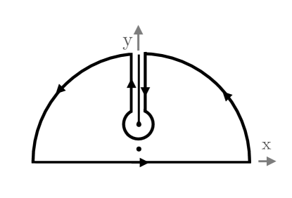
Figure 13: Integration contour.

We define the function of the complex variable $\eta$

$$f(\eta)={\rm e}^{i\,\eta\lambda}\,\frac{\eta}{\eta^{2}+a^{2}}\,\,{\rm ln}\left[(\eta-i\,\alpha_{z})(\eta+i\,\alpha_{z})\right]\ .$$ (71)

This function has branch points at $\eta=\pm\,i\,\alpha_{z}$ and simple poles at $\eta=\pm\,i\,a$ ($0<a\leq 1$), but is otherwise analytic. The upper cut is taken from $i\,\alpha_{z}$ to $+i\,\infty$ (along the positive imaginary axis), while the lower one from $-i\,\alpha_{z}$ to $-i\,\infty$ (along the negative imaginary axis). We consider the closed contour $C$ as in Fig. 13, so that

$$\oint_{C}d\eta\,f(\eta)=2\pi\,i\,{\rm Res}\,f(\eta)\mid_{\eta=i\,a}\ .$$ (72)

Before evaluating the integral above, we need to consider the values of $f(\eta)$ to the right and left of the cut running along the positive imaginary axis. To this end, we define

$$\eta-i\,\alpha_{z}=r_{+}\,{\rm e}^{i\,\theta_{+}}\,\,\,{\rm with}\,\,\,-\frac{3\,\pi}{2}\leq\theta_{+}\leq\frac{\pi}{2}\ ,\qquad\eta+i\,\alpha_{z}=r_{-}\,{\rm e}^{i\,\theta_{-}}\,\,\,{\rm with}\,\,\,-\frac{\pi}{2}\leq\theta_{-}\leq\frac{3\,\pi}{2}\ ,$$ (73)

the restrictions on $\theta_{\pm}$ ensuring that the cuts are not crossed. For a given $\eta$, the difference along the upper cut (corresponding to $\eta=i\,y$ with $y\geq\alpha_{z}$) is given by

$${\rm ln}\left(\eta^{2}+\alpha^{2}_{z}\right)\mid_{{\rm left\,\,\,of\,\,\,cut}}-{\rm ln}\left(\eta^{2}+\alpha^{2}_{z}\right)\mid_{{\rm right\,\,\,of\,\,\,cut}}=-\,2\,\pi\,i\ .$$ (74)

The contributions of the big arcs of radius $R$ and small circle of radius $r$ around the brach point $+\,i\,\alpha_{z}$ vanish as, respectively, $R\rightarrow\infty$ and $r\rightarrow 0$, while on the segments left and right of the upper cut we find

$$\int_{\rm left}d\eta\,f(\eta)-\int_{\rm right}d\eta\,f(\eta)=-2\,\pi\,i\int_{\alpha_{z}}^{\infty}dy\,{\rm e}^{-y\,\lambda}\,\frac{y}{y^{2}-a^{2}}\ .$$ (75)

Therefore from Eq. (72), after evaluating the residue, we arrive at

$$I(z,\lambda)-2\,\pi\int_{\alpha_{z}}^{\infty}dy\,{\rm e}^{-y\,\lambda}\,\frac{y}{y^{2}-a^{2}}=\pi\,{\rm e}^{-a\lambda}\,{\rm ln}(\alpha_{z}^{2}-a^{2})\ ,$$ (76)

from which we deduce

$$\int_{-\infty}^{\infty}dx\,x\,{\rm sin}(x\lambda)\,\frac{G^{\star}(x)}{x^{2}+a^{2}}=2\,\pi\int_{0}^{1}\!\!dz\,\int_{\alpha_{z}}^{\infty}\!dy\,{\rm e}^{-y\,\lambda}\,\frac{y}{y^{2}-a^{2}}+\,\pi\,{\rm e}^{-a\lambda}\int_{0}^{1}\!\!dz\left[{\rm ln}\left(1-z^{2}\right)+{\rm ln}\left(\frac{1}{1-z^{2}}-a^{2}\right)\right]\ .$$ (77)

The first term on the r.h.s. of the equation above can be expressed in terms of exponential functions by noting that

$$\int_{\alpha_{z}}^{\infty}dy\,{\rm e}^{-y\,\lambda}\,\frac{y}{y^{2}-a^{2}}=\frac{{\rm e}^{-a\lambda}}{2}\,E_{1}\left(\lambda\,\alpha_{z}-\lambda\,a\right)+\frac{{\rm e}^{a\lambda}}{2}\,E_{1}\left(\lambda\,\alpha_{z}+\lambda\,a\right)\ ,$$ (78)

so that

$$\int_{-\infty}^{\infty}dx\,x\,{\rm sin}(x\lambda)\,\frac{G^{\star}(x)}{x^{2}+a^{2}} = \pi\int_{0}^{1}dz\,\Big{[}{\rm e}^{-a\lambda}\,E_{1}\left(\lambda\,\alpha_{z}-\lambda\,a\right)+{\rm e}^{a\lambda}\,E_{1}\left(\lambda\,\alpha_{z}+\lambda\,a\right)\Big{]}$$ (79)

$$+\,2\,\pi\,{\rm e}^{-a\lambda}\left(\frac{\sqrt{1-a^{2}}}{a}\,{\rm arctan}\frac{a}{\sqrt{1-a^{2}}}-1\right)\ .$$

A.2 Correlation functions

Inserting the expressions above, we find the Fourier transforms of $\widetilde{F}_{0}(k)$ and $\widetilde{F}_{2}(k)/k^{2}$ to be given by

$$F_{0}^{(0)}(\lambda)\!=\!\int_{\bf k}{\rm e}^{i{\bf k}\cdot{\bf r}}\,\widetilde{F}_{0}(k)=\frac{g_{A}^{4}}{256\,\pi^{3}}\,\frac{\left(2\,m_{\pi}\right)^{4}}{f_{\pi}^{4}}\bigg{\{}\frac{{\rm e}^{-\lambda}}{\lambda}\left[1+\frac{1}{2}\int_{0}^{1}dz\,\frac{1-{\rm e}^{-\lambda(\alpha_{z}-1)}}{\alpha_{z}^{2}-1}\right]-\left[\left(\frac{1}{g_{A}^{2}}+1\right)\frac{1}{\lambda}-\frac{1}{2}\right]E^{(-)}_{1}(\lambda)$$

$$\hskip 199.16928pt-\left[\left(\frac{1}{g_{A}^{2}}+1\right)\frac{1}{\lambda}+\frac{1}{2}\right]E^{(+)}_{1}(\lambda)\bigg{\}}\ ,$$ (80)

$$F^{(0)}_{2}(\lambda)\!=\!(2\,m_{\pi})^{2}\!\int_{\bf k}{\rm e}^{i{\bf k}\cdot{\bf r}}\,\frac{\widetilde{F}_{2}(k)}{k^{2}}=-\frac{g_{A}^{4}}{256\,\pi^{3}}\,\frac{\left(2\,m_{\pi}\right)^{4}}{f_{\pi}^{4}}\bigg{\{}\frac{{\rm e}^{-\lambda}}{\lambda}\left[1+\frac{1}{2}\int_{0}^{1}dz\,\frac{1-{\rm e}^{-\lambda(\alpha_{z}-1)}}{\alpha_{z}^{2}-1}\right]-\left[\left(\frac{1}{g_{A}^{2}}+2\right)\frac{1}{\lambda}-\frac{1}{2}\right]\!E^{(-)}_{1}(\lambda)$$

$$\hskip 199.16928pt-\left[\left(\frac{1}{g_{A}^{2}}+2\right)\frac{1}{\lambda}+\frac{1}{2}\right]\!E^{(+)}_{1}(\lambda)+\left(\frac{1}{g_{A}^{2}}-2\right)\frac{1}{\lambda}\,E_{1}^{(0)}(\lambda)\bigg{\}}\ ,$$ (81)

where we have defined

$$E_{1}^{(\pm)}(\lambda)=\frac{{\rm e}^{\pm\lambda}}{2}\int_{0}^{1}dz\,E_{1}\left(\lambda\,\alpha_{z}\pm\lambda\right)\ ,\qquad E_{1}^{(0)}(\lambda)=\int_{0}^{1}dz\,E_{1}\left(\lambda\,\alpha_{z}\right)\ .$$ (82)

The correlation functions $F_{2}^{(1)}(\lambda)$ and $F_{2}^{(2)}(\lambda)$ in Eq. (13) are obtained as

$$F_{2}^{(1)}(\lambda)=\frac{1}{\lambda}\,\frac{d}{d\lambda}F^{(0)}_{2}(\lambda) = \frac{g_{A}^{4}}{256\,\pi^{3}}\,\frac{\left(2\,m_{\pi}\right)^{4}}{f_{\pi}^{4}}\bigg{\{}{\rm e}^{-\lambda}\left(\frac{1}{\lambda^{3}}+\frac{1}{\lambda^{2}}\right)\left[1+\frac{1}{2}\int_{0}^{1}dz\,\frac{1-{\rm e}^{-\lambda(\alpha_{z}-1)}}{\alpha_{z}^{2}-1}\right]$$ (83)

$$-\left[\left(\frac{1}{g_{A}^{2}}+2\right)\left(\frac{1}{\lambda^{3}}+\frac{1}{\lambda^{2}}\right)-\frac{1}{2\,\lambda}\right]\!E_{1}^{(-)}(\lambda)-\left[\left(\frac{1}{g_{A}^{2}}+2\right)\left(\frac{1}{\lambda^{3}}-\frac{1}{\lambda^{2}}\right)-\frac{1}{2\,\lambda}\right]\!E_{1}^{(+)}(\lambda)$$

$$+\left(\frac{1}{g_{A}^{2}}-2\right)\,\frac{1}{\lambda^{3}}\,E_{1}^{(0)}(\lambda)-\int_{0}^{1}dz\left(\frac{4}{\lambda^{3}}+\frac{1}{\alpha_{z}+1}\,\frac{1}{2\,\lambda^{2}}\right){\rm e}^{-\lambda\alpha_{z}}\bigg{\}}\ ,$$

$$F_{2}^{(2)}(\lambda) = \frac{d^{2}}{d\lambda^{2}}F^{(0)}_{2}(\lambda)-\frac{1}{\lambda}\,\frac{d}{d\lambda}F^{(0)}_{2}(\lambda)=-\frac{g_{A}^{4}}{256\,\pi^{3}}\,\frac{\left(2\,m_{\pi}\right)^{4}}{f_{\pi}^{4}}\bigg{\{}{\rm e}^{-\lambda}\left(\frac{3}{\lambda^{3}}+\frac{3}{\lambda^{2}}+\frac{1}{\lambda}\right)\left[1+\frac{1}{2}\int_{0}^{1}dz\,\frac{1-{\rm e}^{-\lambda(\alpha_{z}-1)}}{\alpha_{z}^{2}-1}\right]$$ (84)

$$\hskip 85.35826pt-\left[\left(\frac{1}{g_{A}^{2}}+2\right)\left(\frac{3}{\lambda^{3}}+\frac{3}{\lambda^{2}}+\frac{1}{\lambda}\right)-\frac{1}{2}\left(1+\frac{1}{\lambda}\right)\right]\!E_{1}^{(-)}(\lambda)$$

$$\hskip 85.35826pt-\left[\left(\frac{1}{g_{A}^{2}}+2\right)\left(\frac{3}{\lambda^{3}}-\frac{3}{\lambda^{2}}+\frac{1}{\lambda}\right)+\frac{1}{2}\left(1-\frac{1}{\lambda}\right)\right]\!E_{1}^{(+)}(\lambda)+\left(\frac{1}{g_{A}^{2}}-2\right)\frac{3}{\lambda^{3}}\,E_{1}^{(0)}(\lambda)$$

$$\hskip 85.35826pt-\int_{0}^{1}dz\left[\frac{16}{\lambda^{3}}+\left(4\,\alpha_{z}+\frac{3}{2}\,\frac{1}{\alpha_{z}+1}\right)\frac{1}{\lambda^{2}}\right]{\rm e}^{-\lambda\alpha_{z}}\bigg{\}}\ .$$

References

• (1) A. Gezerlis, I. Tews, E. Epelbaum, S. Gandolfi, K. Hebeler, A. Nogga, and A. Schwenk, Phys. Rev. Lett. 111, 032501 (2013).
• (2) M. Piarulli, L. Girlanda, R. Schiavilla, R. Navarro Pérez, J.E. Amaro, and E. Ruiz Arriola, Phys. Rev. C 91, 024003 (2015).
• (3) M. Piarulli, L. Girlanda, R. Schiavilla, A. Kievsky, A. Lovato, L.E. Marcucci, S.C. Pieper, M. Viviani, and R.B. Wiringa, Phys. Rev. C 94, 054007 (2016).
• (4) A. Gezerlis, I. Tews, E. Epelbaum, M. Freunek, S. Gandolfi, K. Hebeler, A. Nogga, and A. Schwenk, Phys. Rev. C 90, 054323 (2014).
• (5) J.E. Lynn, J. Carlson, E. Epelbaum, S. Gandolfi, A. Gezerlis, and A. Schwenk, Phys. Rev. Lett. 113, 192501 (2014).
• (6) J.E. Lynn, I. Tews, J. Carlson, S. Gandolfi, A. Gezerlis, K.E. Schmidt, and A. Schwenk, Phys. Rev. Lett. 116, 062501 (2016).
• (7) I. Tews, S. Gandolfi, A. Gezerlis, and A.  Schwenk, Phys. Rev. C 93, 024305 (2016).
• (8) S. Gandolfi, H.W. Hammer, P. Klos, J.E. Lynn, and A.  Schwenk, Phys. Rev. Lett. 118, 232501 (2017).
• (9) J.E. Lynn, I. Tews, J. Carlson, S. Gandolfi, A. Gezerlis, K.E. Schmidt, and A. Schwenk, Phys. Rev. C 96, 054007 (2017).
• (10) M. Piarulli, A. Baroni, L. Girlanda, A. Kievsky, A. Lovato, E. Lusk, L.E. Marcucci, S.C. Pieper, R. Schiavilla, M. Viviani, and R.B. Wiringa, Phys. Rev. Lett. 120, 052503 (2018).
• (11) E. Epelbaum, A. Nogga, W. Gloeckle, H. Kamada, U.-G. Meissner, and H. Witala, Phys. Rev. C 66, 064001 (2002).
• (12) D. Gazit, S. Quaglioni, and P. Navratil, Phys. Rev. Lett. 103, 102502 (2009).
• (13) L.E. Marcucci, A. Kievsky, S. Rosati, R. Schiavilla, and M. Viviani, Phys. Rev. Lett. 108, 052502 (2012); 121, 049901(E) (2018).
• (14) A. Baroni, R. Schiavilla, L.E. Marcucci, L. Girlanda, A. Kievsky, A. Lovato, S. Pastore, M. Piarulli, S.C. Pieper, M. Viviani, and R.B. Wiringa, Phys. Rev. C in press; arXiv:1806.10245.
• (15) A. Gardestig and D.R. Phillips, Phys. Rev. Lett. 96, 232301 (2006).
• (16) R. Schiavilla, unpublished.
• (17) N. Fettes, U.-G. Meissner, M. Mojzis, and S. Steininger, Ann. Phys. (N.Y.) 283, 273 (2000).
• (18) H. Krebs, E. Epelbaum, and U.-G. Meissner, Eur. Phys. J. A 32, 127 (2007).
• (19) R. Navarro Pérez, J.E. Amaro, and E. Ruiz Arriola, Phys. Rev. C 88, 024002 (2013); 88, 069902(E) (2013).
• (20) A. Lovato, M. Piarulli, and R.B. Wiringa, unpublished.
• (21) P.B. Demorest, T. Pennucci, S.M. Ransom, M.S.E. Roberts, and J.W.T. Hessels, Nature  467, 1081 (2010).
• (22) J. Antoniadis et al., Science  340, 1233232 (2013).
• (23) S.R. Beane, E. Chang, S. Cohen, W. Detmold, H.W. Lin, K. Orginos, A. Parreno, M.J. Savage, and B.C. Tiburzi (NPLQCD Collaboration), Phys. Rev. Lett. 113, 252001 (2014).
• (24) T.-S. Park, D.-P. Min, and M. Rho, Phys. Rep. 233, 341 (1993).
• (25) T.-S. Park, D.-P. Min, and M. Rho, Nucl. Phys. A596, 515 (1996).
• (26) S. Pastore, L. Girlanda, R. Schiavilla, M. Viviani, and R.B. Wiringa, Phys. Rev. C 80, 034004 (2009).
• (27) S. Pastore, L. Girlanda, R. Schiavilla, and M. Viviani, Phys. Rev. C 84, 024001 (2011).
• (28) M. Piarulli, L. Girlanda, L.E. Marcucci, S. Pastore, R. Schiavilla, and M. Viviani, Phys. Rev. C 87, 014006 (2013).
• (29) S. Kölling, E. Epelbaum, H. Krebs, and U.-G. Meissner, Phys. Rev. C 80, 045502 (2009).
• (30) S. Kölling, E. Epelbaum, H. Krebs, and U.-G. Meissner, Phys. Rev. C 84, 054008 (2011).
• (31) S. Okubo, Prog. Theor. Phys. 12, 603 (1954).
• (32) S. Pastore, R. Schiavilla, and J.L. Goity, Phys. Rev. C 78, 064002 (2008).
• (33) L.E. Marcucci, D.O. Riska, and R. Schiavilla, Phys. Rev. C 58, 3069 (1998).
• (34) R. Schiavilla, R.B. Wiringa, V.R. Pandharipande, and J. Carlson, Phys. Rev. C 45, 2628 (1992).
• (35) C.E. Carlson, Phys. Rev. D 34, 2704 (1986).
• (36) L. Girlanda, A. Kievsky, L.E. Marcucci, S. Pastore, R. Schiavilla, and M. Viviani, Phys. Rev. Lett. 105, 232502 (2010).
• (37) A. Kievsky, S. Rosati, M. Viviani, L.E. Marcucci, and L. Girlanda, J. Phys. G 35, 063101 (2008).
• (38) J. Carlson, S. Gandolfi, F. Pederiva, S.C. Pieper, R. Schiavilla, K.E. Schmidt, and R.B. Wiringa, Rev. Mod. Phys. 87, 1067 (2015).
• (39) N. Metropolis, A.W. Rosenbluth, M.N. Rosenbluth, A.H. Teller, and E. Teller, J. Chem.  Phys. 21 (6), 1087 (1953).
• (40) L.E. Marcucci, F. Gross, M.T. Pena, M. Piarulli, R. Schiavilla, I. Sick, A. Stadler, J.W. Van Orden, and M. Viviani, J. Phys. G43, 023002 (2016).
• (41) G.R. Bishop, C.H. Collie, H. Halban, A. Hedgran, K. Siegbahn, S. du Toit, and R. Wilson, Phys. Rev. 80, 211 (1950); Phys. Rev. 81, 644(E) (1951).
• (42) A.H. Snell, E.C. Barker, and R.L. Sternberg, Phys. Rev. 80, 637 (1950).
• (43) S.A. Colgate, Phys. Rev. 83, 1262 (1951).
• (44) J.H. Carver and D.H. Wilkinson, Nature (London) 167, 154 (1951).
• (45) Y. Birenbaum, S. Kahane, and R. Moreh, Phys. Rev. C 32, 1825 (1985).
• (46) R. Moreh, T.J. Kennett, and W.V. Prestwich, Phys. Rev. C 39, 1247 (1989).
• (47) A. De Graeve et al., Phys. Rev. C 45, 860 (1992).
• (48) R.E. Rand, R.F. Frosch, C.E. Littig, and M.R. Yearian. Phys. Rev. Lett. 18, 469 (1967).
• (49) D. Ganichot, B. Grossetête, and D.B. Isabelle, Nucl. Phys. A178, 545 (1972).
• (50) G.G. Simon, F. Borkowski, Ch. Schmitt, V.H. Walther, H. Arenhövel, and W. Fabian, Nucl. Phys. A324, 277 (1979).
• (51) M. Bernheim, E. Jans, J. Mougey, D. Royer, D. Tarnowski, S. Turck-Chieze, I. Sick, G.P. Capitani, E. De Sanctis, and S. Frullani, Phys. Rev. Lett. 46, 402 (1981).
• (52) D. Auffret et al., Phys. Rev. Lett. 55, 1362 (1985).
• (53) W.M. Schmitt et al., Phys. Rev. C 56, 1687 (1997).
• (54) R.G. Arnold et al., Phys. Rev. C 42, R1 (1990).
• (55) M. Frodyma et al., Phys. Rev. C 47, 1599 (1993).
• (56) B. Kubis and U.-G. Meissner, Nucl. Phys.  A679, 698 (2001).
• (57) R. Schiavilla and V.R. Pandharipande, Phys. Rev. C 65, 064009 (2002).
• (58) R.B. Wiringa, V.G.J. Stoks, and R. Schiavilla, Phys. Rev. C 51, 38 (1995).
• (59) D.R. Entem and R. Machleidt, Phys. Rev. C 68, 041001 (2003).
• (60) R. Machleidt and D.R. Entem, Phys. Rep. 503, 1 (2011).
• (61) J. Carlson and R. Schiavilla, Rev. Mod. Phys. 70, 743 (1998).
• (62) R. Schiavilla, Phys. Rev. C 72, 034001 (2005).
• (63) R. Schiavilla, J. Carlson, and M. Paris, Phys. Rev. C 70, 044007 (2004).
• (64) J. Hockert, D.O. Riska, M. Gari, and A. Huffman, Nucl. Phys. A217, 14 (1973).
• (65) R. Schiavilla and D.O. Riska, Phys. Rev.  C 43, 437 (1991).
• (66) M. Abramovitz and I.A. Stegun, Handbook of Mathematical Functions, U.S. Government Printing Office Washington, D.C. 20402 (1972).