On the asymptotic stability of the time–fractional Lengyel–Epstein system

Abstract

This paper concerns a time fractional version of the conventional Lengyel–Epstein CIMA reaction model. We define the invariant regions of the system and establish sufficient conditions for the unique equilibrium’s local and global asymptotic stability. Numerical results are presented to illustrate the effect of the fractional order on system dynamics.

1 Introduction

In this paper, we are interested in a fractional version of the Lengyel–Epstein reaction–diffusion system proposed in [1, 2] as a model of the chlorite–iodide malonic–acid (CIMA) chemical reaction [3]. The considered model has attracted the interest of many researchers since its inception in 1991. The reason for this interest is the fact that the CIMA reaction is one of the earliest experiments that confirmed the theoretical propositions of Alan Turing in 1952 [4] concerning the chemical basis for morphogenesis and more generally pattern formation. The CIMA reaction can be described by three chemical reaction schemes as follows

$$\left\{\begin{array}[]{l}MA+I_{2}\rightarrow IMA+I^{-}+H^{+},\\ CIO_{2}+I^{-}\rightarrow\frac{1}{2}I_{2}+CIO_{2}^{-},\\ CIO_{2}^{-}+4I^{-}+4H^{+}\rightarrow CI^{-}+2I_{2}+2H_{2}O.\end{array}\right.$$ (1.1)

Considering the empirical rate laws corresponding to these processes and ignoring constant factors, the model for this reaction was reduced to the conventional Lengyel–Epstein model with two dependent variables $u$ and $v$ representing the time evolution of the concentrations of $\left[I^{-}\right]$ and $\left[CIO_{2}^{-}\right]$, respectively. The general dynamics of the Lengyel–Epstein system have been examined in a number of studies. Sufficient conditions for its local and global asymptotic stability can be found in [5, 6, 7, 8]. In [6, 9], the authors establish sufficient conditions for the Turing or diffusion–driven instability of the system. More details on the formation of patterns in the Lengyel–Epstein model can be found in [10]. Also, results related to the Hopf–bifurcation for the Lengyel–Epstein system are presented and analyzed in [11, 6, 9]. In addition, many studies have also examined modified versions of the system including [12, 13, 14, 15, 16, 17, 18, 19, 20, 21, 22, 23, 24] with the aim of relaxing existing asymptotic stability and Turing instability conditions.

In [25], the authors considered the model

$$\left\{\begin{array}[]{l}\dfrac{\partial u}{\partial t}=\nabla^{\gamma}u+a-u-\dfrac{4uv}{1+u^{2}},\\ \dfrac{\partial v}{\partial t}=\sigma\left[c\nabla^{\gamma}v+b\left(u-\dfrac{uv}{1+u^{2}}\right)\right],\end{array}\right.$$ (1.2)

which accounts for anomalous diffusion in a fractal medium for example. The term $\nabla^{\gamma}$ denotes the Riesz fractional operator with $1<\gamma<2$. The authors established sufficient conditions for the existence of Turing patterns and examined their nature. Note that system (1.2) is fractional in the spatial sense. In our work, we aim to propose and study the dynamics of the time–fractional system corresponding to the Lengyel–Epstein model.

The following section states some of the necessary notation and theory related to fractional systems. Section 3 describes the proposed system and examines its invariant regions. Section 4 establishes conditions for the asymptotic stability of the proposed system. Section 5 illustrates the analytical conditions through numerical examples. Finally, Section 6 summarizes the findings of this study and poses open questions for future investigation.

2 Fractional Calculus

In this section, we start with some of the necessary notation and stability theory related to the subject.

Definition 1

[34] The Riemann–Liouville fractional derivative of order $\delta$ of an integrable function $f\left(t\right)$ is defined as

$${}_{t_{0}}D_{t}^{-\delta}f\left(t\right)=\frac{1}{\Gamma\left(\delta\right)}\int_{t_{0}}^{t}\frac{f\left(\tau\right)}{\left(t-\tau\right)^{1-\delta}}d\tau.$$ (2.1)

where $0<\delta\in\mathbb{R}^{+}$ and $\Gamma\left(\delta\right)=\int_{0}^{\infty}e^{-t}t^{\delta-1}dt$ is the Gamma function.

Definition 2

[26] The Caputo fractional derivative of order $\delta>0$ of a function $f\$of class $C^{n}$ for $t>t_{0}$ is defined as

$${}_{t_{0}}^{C}D_{t}^{\delta}f\left(t\right)=\frac{1}{\Gamma\left(n-\delta\right)}\int_{t_{0}}^{t}\frac{f^{\left(n\right)}\left(\tau\right)}{\left(t-\tau\right)^{\delta-n-1}}d\tau,$$ (2.2)

with $n=\min\left\{k\in\mathbb{N}\ |\ k>\delta\right\}$ and $\Gamma$ representing the gamma function.

Note that the constant $\left(u^{\ast},v^{\ast}\right)$ is an equilibrium for the Caputo fractional non–autonomous dynamic system

$$\left\{\begin{array}[]{l}{}_{t_{0}}^{C}D_{t}^{\delta}u=F\left(u,v\right),\text{ \ \ \ \ \ \ in }\mathbb{R}^{+},\vskip 6.0pt plus 2.0pt minus 2.0pt\\ {}_{t_{0}}^{C}D_{t}^{\delta}v=G\left(u,v\right),\text{ \ \ \ \ \ in }\mathbb{R}^{+},\end{array}\right.$$ (2.3)

if and only if

$$F\left(u^{\ast},v^{\ast}\right)=G\left(u^{\ast},v^{\ast}\right)=0.$$ (2.4)

The following lemmas hold.

Lemma 1

Let $u\left(t\right)$ be a continuous and differentiable real function. For any time instant $t\geq t_{0}$,

$${}_{t_{0}}^{C}D_{t}^{\delta}u^{2}\left(t\right)\leq 2u\left(t\right)_{t_{0}}^{C}D_{t}^{\delta}u\left(t\right),$$ (2.5)

with $\delta\in\left(0,1\right]$.

Lemma 2

[29] An equilibrium point $\left(u^{\ast},v^{\ast}\right)$ of (2.3) is locally asymptotically stable iff

$$\left|\arg\left(\lambda_{i}\right)\right|>\frac{\delta\pi}{2},\ \ \ i=1,2,$$ (2.6)

where $\lambda_{i}$ are the eigenvalues of the Jacobian matrix $J\left(u^{\ast},v^{\ast}\right)$ and $\arg\left(\cdot\right)$ denotes the argument of a complex number.

Lemma 3

If an equilibrium point $\left(u^{\ast},v^{\ast}\right)$ of (2.3) is locally asymptotically stable for the standard system

$$\left\{\begin{array}[]{l}u_{t}=F\left(u,v\right),\text{ \ \ \ \ \ \ in }\mathbb{R}^{+},\vskip 6.0pt plus 2.0pt minus 2.0pt\\ v_{t}=G\left(u,v\right),\text{ \ \ \ \ \ in }\mathbb{R}^{+},\end{array}\right.$$ (2.7)

then, it is also locally asymptotically stable for (2.3).

Proof 1

Assuming that $\left(u^{\ast},v^{\ast}\right)$ is a locally asymptotically stable equilibrium for (2.7), then all the eigenvalues of the Jacobian matrix have negative real parts, i.e.

$$\left|\arg\left(\lambda_{i}\right)\right|>\frac{\pi}{2},\ \ \ i=1,2.$$

Since $\delta<1$, it is trivial to see that (2.6) holds, which leads to the local asymptotic stability of $\left(u^{\ast},v^{\ast}\right)$ as an equilibrium of (2.3).

Corollary 1

In the diffusion case, if an equilibrium point $\left(u^{\ast},v^{\ast}\right)$ of (2.3) is locally asymptotically stable for the integer system

$$\left\{\begin{array}[]{l}u_{t}-d_{1}\Delta u=F\left(u,v\right),\text{ \ \ \ \ \ \ in }\mathbb{R}^{+}\times\Omega,\vskip 6.0pt plus 2.0pt minus 2.0pt\\ v_{t}-d_{2}\Delta v=G\left(u,v\right),\text{ \ \ \ \ \ in }\mathbb{R}^{+}\times\Omega,\end{array}\right.$$

then it is also locally asymptotically stable for

$$\left\{\begin{array}[]{l}{}_{0}^{C}D_{t}^{\delta}u-d_{1}\Delta u=F\left(u,v\right),\text{ \ \ \ \ \ \ in }\mathbb{R}^{+}\times\Omega,\vskip 6.0pt plus 2.0pt minus 2.0pt\\ {}_{0}^{C}D_{t}^{\delta}v-d_{2}\Delta v=G\left(u,v\right),\text{ \ \ \ in }\mathbb{R}^{+}\times\Omega.\end{array}\right.$$

3 System Model

In this paper, we consider the time fractional Lengyel–Epstein system

$$\left\{\begin{array}[]{l}{}_{0}^{C}D_{t}^{\delta}u-d_{1}\Delta u=a-u-\frac{4uv}{1+u^{2}}=:F\left(u,v\right),\text{ \ \ \ \ \ \ in }\mathbb{R}^{+}\times\Omega,\vskip 6.0pt plus 2.0pt minus 2.0pt\\ {}_{0}^{C}D_{t}^{\delta}v-d_{2}\Delta v=\sigma b\left(u-\frac{uv}{1+u^{2}}\right)=:G\left(u,v\right),\text{ \ \ \ in }\mathbb{R}^{+}\times\Omega,\end{array}\right.$$ (3.1)

where $\Omega$ is a bounded domain in $\mathbb{R}^{n}$ ($n=2,3$ in practice) with smooth boundary $\partial\Omega$, $\Delta=\underset{i=1}{\overset{n}{\sum}}\frac{\partial^{2}}{\partial x_{i}^{2}}$, $0<\delta\leq 1$ is the fractional order, ${}_{0}^{C}D_{t}^{\delta}$ denotes the Caputo fractional derivative over $\left(0,\infty\right)$ as defined in (2.2), and $d_{1},d_{2},a$ and $\sigma$ are strictly positive constants. We assume the nonnegative initial conditions

$$0\leq u\left(0,x\right)=u_{0}\left(x\right),\text{ \ }0\leq v\left(0,x\right)=v_{0}\left(x\right),\text{\ \ \ \ in }\Omega,$$ (3.2)

with $u_{0},v_{0}\in C^{2}\left(\Omega\right)\cap C\left(\overline{\Omega}\right)$, and impose homogeneous Neumann boundary conditions

$$\dfrac{\partial u}{\partial\nu}=\dfrac{\partial v}{\partial\nu}=0\ \ \text{\ \ \ \ \ on \ \ \ }\mathbb{R}^{+}\times\partial\Omega,$$ (3.3)

where $\nu$ is the unit outer normal to $\partial\Omega$.

Before we study the local and global asymptotic stability of the solutions of the proposed system, let us define its invariant region. We start with a definition of the term invariant region following the lines of [31, 7]. Note that when $F\left(u,v\right)=0$, the curves in the $u$–$v$ plane are called $u$–isoclines. Similarly, they are called $v$–isoclines when $G\left(u,v\right)=0$. in addition, if the vector field $\left(F,G\right)$ does not point outwards at the boundary of a certain rectabgle $\partial\Re$, then $\Re$ is said to be an invariant rectangle. This is similar to following definition.

Definition 3

A rectangle $\Re$ is said to be an invariant rectangle if the vector field $\left(F,G\right)$ on the boundary $\partial\Re$ points inside, i.e.

$$\left\{\begin{array}[]{l}F\left(0,v\right)\geq 0\text{ and }F\left(r_{1},v\right)\leq 0\text{ for }0<v<r_{2},\vskip 6.0pt plus 2.0pt minus 2.0pt\\ G\left(u,0\right)\geq 0\text{ and }G\left(u,r_{2}\right)\leq 0\text{ for }0<u<r_{1}.\end{array}\right.$$ (3.4)

The following proposition describes the invariant region of the proposed system (3.1).

Proposition 1

System (3.1) admits the region of attraction

$$\Re_{a}=\left(0,a\right)\times\left(0,1+a^{2}\right).$$ (3.5)

4 Asymptotic Stability Conditions

4.1 Local Stability

In this section, we derive sufficient conditions for the local asymptotic stability of the equilibrium point of (3.1). The free diffusions system corresponding to (3.1) is

$$\left\{\begin{array}[]{l}{}_{0}^{C}D_{t}^{\delta}u=a-u-\frac{4uv}{1+u^{2}},\vskip 6.0pt plus 2.0pt minus 2.0pt\\ {}_{0}^{C}D_{t}^{\delta}v=\sigma b\left(u-\frac{uv}{1+u^{2}}\right).\end{array}\right.$$ (4.1)

Proposition 2

System (4.1) has the unique equilibrium

$$\left(u^{\ast},v^{\ast}\right)=\left(\alpha,1+\alpha^{2}\right),$$ (4.2)

with

$$\alpha=\frac{a}{5}.$$ (4.3)

Subject to

$$\Upsilon=\left(\frac{3\alpha^{2}-5-\sigma b\alpha}{1+\alpha^{2}}\right)^{2}-20\frac{\sigma b\alpha}{\alpha^{2}+1}\geq 0,$$

$\left(u^{\ast},v^{\ast}\right)$ is asymptotically stable if

$$\text{tr}J<0,$$

and unstable if

$$\text{tr}J>0,$$

where

$$J=\left(\begin{array}[]{cc}\frac{3\alpha^{2}-5}{1+\alpha^{2}}&-\frac{4\alpha}{1+\alpha^{2}}\\ \sigma b\frac{2\alpha^{2}}{1+\alpha^{2}}&-\sigma b\frac{\alpha}{1+\alpha^{2}}\end{array}\right).$$

Alternatively, if $\Upsilon<0$, then $\left(u^{\ast},v^{\ast}\right)$ is asymptotically stable whenever tr$J\leq 0$ or

$$\left|\arg\left(\lambda_{1}\right)\right|>\delta\frac{\pi}{2}\text{ and }\left|\arg\left(\lambda_{2}\right)\right|>\delta\frac{\pi}{2},$$ (4.4)

where

$$\lambda_{1,2}=\frac{1}{2}\left[\frac{3\alpha^{2}-5-\sigma b\alpha}{1+\alpha^{2}}\pm i\sqrt{-\Upsilon}\right].$$ (4.5)

Proof 2

The Jacobian matrix in $\left(u^{\ast},v^{\ast}\right)$ is given by

$$J\left(u^{\ast},v^{\ast}\right)=\left(\begin{array}[]{cc}\frac{3\alpha^{2}-5}{1+\alpha^{2}}&-\frac{4\alpha}{1+\alpha^{2}}\\ \sigma b\frac{2\alpha^{2}}{1+\alpha^{2}}&-\sigma b\frac{\alpha}{1+\alpha^{2}}\end{array}\right).$$

Its determinant and trace are given by

$$\det J\left(u^{\ast},v^{\ast}\right)=5\sigma b\frac{\alpha}{\alpha^{2}+1},$$

and

$$\text{tr}J\left(u^{\ast},v^{\ast}\right)=\frac{3\alpha^{2}-5-\sigma b\alpha}{1+\alpha^{2}},$$

respectively.

The characteristic equation of the Jacobian matrix is

$$\lambda^{2}-\left(\text{tr}J\right)\lambda+\det J=0,$$

and its discriminant is

$$\Upsilon=\left(\text{tr}J\right)^{2}-4\det J.$$

We study the different cases separately. First, if $\Upsilon>0$, then the eigenvalues $\lambda_{1,2}$ are real and can be rewritten as

$$\lambda_{1,2}=\frac{1}{2}\left[\text{tr}J\pm\sqrt{\Upsilon}\right].$$

Note that $\det J>0$. Hence, the negativity of the eigenvalues rests on the sign of the trace $\text{tr}J$:

• If $\text{tr}J<0$, then

  $$\lambda_{1}=\frac{1}{2}\left[\text{tr}J-\sqrt{\Upsilon}\right]<0,$$

  and, therefore, $\arg\left(\lambda_{1}\right)=\pi$. Since both eigenvalues are real, the trace is negative, and the determinant is positive, it is evident that $\left|\arg\left(\lambda_{2}\right)\right|=\left|\arg\left(\lambda_{1}\right)\right|=\pi>\frac{\delta\pi}{2}$ as $\delta\in\left(0,1\right]$. It follows that the equilibrium $\left(u^{\ast},v^{\ast}\right)$ is asymptotically stable.

• If $\text{tr}J>0$, we have

  $$\text{tr}J-\sqrt{\Upsilon}>0,$$

  leading to

  $$\lambda_{1}=\frac{1}{2}\left[\text{tr}J-\sqrt{\Upsilon}\right]>0,$$

  and thus

  $$\left|\arg\left(\lambda_{1}\right)\right|=0.$$

  So, $\left(u^{\ast},v^{\ast}\right)$ is asymptotically unstable.

• If $\text{tr}J=0$, then

  $$\Upsilon>0\Rightarrow-4\det J>0,$$

  which is a contradiction. Hence, this case does not show up.

Next, we consider the case of the discriminant $\Upsilon$ being equal to zero. Since $\det J>0$, then it is impossible that $\text{tr}J=0$. The eigenvalues reduce to

$$\lambda_{1,2}=\frac{1}{2}\text{tr}J.$$

The sign of the eigenvalues is identical to that of the trace. Consequently, $\left(u^{\ast},v^{\ast}\right)$ is asymptotically stable for all $\delta\in\left(0,1\right]$ if $\text{tr}J<0$ and unstable if $\text{tr}J>0$.

Finally, if the discriminant $\Upsilon<0$, then

$$\lambda_{1,2} =\frac{1}{2}\left[\text{tr}J\pm\sqrt{\Upsilon}\right]$$

$$=\frac{1}{2}\left[\text{tr}J\pm i\sqrt{-\Upsilon}\right].$$

We, now, have three cases:

• If tr$J<0$, then by means of Lemma 3, $\left(u^{\ast},v^{\ast}\right)$ is asymptotically stable.

• If $\text{tr}J=0$, then

  $$\left|\arg\left(\lambda_{1,2}=\pm\frac{1}{2}i\sqrt{-\Upsilon}\right)\right|=\frac{\pi}{2}.$$

  Hence, for $\delta<1$, $\left(u^{\ast},v^{\ast}\right)$ is asymptotically stable.

• If tr$J>0$, then $\left(u^{\ast},v^{\ast}\right)$ is asymptotically stable subject to (4.4).

The proof is complete.

Now, let us move on to the complete system (3.1). For this, we are going to use the eigenfunction expansion method [32]. We denote the eigenvalues of the spectral problem with Neumann boundary conditions by $0=\lambda_{0}\leq\lambda_{1}\leq\lambda_{2}\leq\cdots\leq\lambda_{k}\leq\cdots$ and the corresponding normalized eigenfunctions by $\phi_{0},\cdots,\phi_{k},\cdots$. Let us set

$$J_{i}=\left(\begin{array}[]{cc}F_{0}-d_{1}\lambda_{i}&F_{1}\\ \sigma G_{0}&\sigma G_{1}-d_{2}\lambda_{i}\end{array}\right),$$ (4.6)

and

$$L=\left(\begin{array}[]{cc}d_{1}\Delta+F_{0}&F_{1}\\ \sigma G_{0}&d_{2}\Delta+\sigma G_{1}\end{array}\right),$$ (4.7)

where

$$F_{0}=\frac{3\alpha^{2}-5}{1+\alpha^{2}},\ F_{1}=-\frac{4\alpha}{1+\alpha^{2}},\ G_{0}=b\frac{2\alpha^{2}}{1+\alpha^{2}},\ \text{and}\ G_{1}=-b\frac{\alpha}{1+\alpha^{2}}.$$ (4.8)

In addittion, if $d_{1}>d_{2}$, we define $\lambda_{01}<\lambda_{02}$ as the roots of

$$\Upsilon_{i}=\left(d_{1}-d_{2}\right)^{2}\lambda_{i}^{2}+2\left(d_{1}-d_{2}\right)\left(-F_{0}+\sigma G_{1}\right)\lambda_{i}+\Upsilon.$$ (4.9)

The following proposition describes the conditions for the asymptotic stability of the steady state assuming $F_{0}>0$.

Proposition 3

If $d_{1}=d_{2}$, then the asymptotic stability conditions are identical to the free diffusions case as stated in Proposition 2. Alternatively, if $d_{1}\not=d_{2}$, $\text{tr}J<0$ and $\Upsilon>0$, then $\left(u^{\ast},v^{\ast}\right)$ is an asymptotically stable constant steady state if $d_{1}<d_{2}$ and

$$\left\{\begin{array}[]{lll}\lambda_{1}d_{1}\geq F_{0},&\text{or}&\vskip 6.0pt plus 2.0pt minus 2.0pt\\ \lambda_{1}d_{1}<F_{0}&\text{and}&0<d_{2}<\tilde{d},\end{array}\right.$$ (4.10)

where

$$d_{i}=\sigma b\frac{\alpha}{1+\alpha^{2}}\frac{\left(\lambda_{i}d_{1}+5\right)}{\left(F_{0}-\lambda_{i}d_{1}\right)\lambda_{i}},$$ (4.11)

and

$$\tilde{d}=\min_{i\geq 0}d_{i}.$$ (4.12)

If $d_{1}>d_{2}$, the euilibrium $\left(u^{\ast},v^{\ast}\right)$ is asymptotically stable if $\lambda_{1}d_{1}\geq F_{0}$ and the eigenvalues

$$\xi_{1,2}\left(\lambda_{i}\right)=\frac{1}{2}\left[\text{tr}J_{i}\pm i\sqrt{4\det J_{i}-\left(\text{tr}J_{i}\right)^{2}}\right]$$ (4.13)

satisfy

$$\left|\arg\left(\xi_{1}\left(\lambda_{i}\right)\right)\right|>\delta\frac{\pi}{2}\text{ and }\left|\arg\left(\xi_{2}\left(\lambda_{i}\right)\right)\right|>\delta\frac{\pi}{2}$$ (4.14)

for all $\lambda_{i}\in\left(\lambda_{01},\lambda_{02}\right)$.

Proof 3

In order to study the local asymptotic stability in the PDE sense, we will linearize the system. Following the standard linear operator theory (see [32]), and keeping in mind the fractional nature of the system, we can state that $\left(u^{\ast},v^{\ast}\right)$ is asymptotically stable if the eigenvalues of the linearized system satisfy the conditions of Lemma 2.

Suppose that $\left(\phi\left(x\right),\psi\left(x\right)\right)$ is an eigenfunction of $L$ corresponding to the eigenvalue $\xi$. Then,

$$\left(\begin{array}[]{cc}d_{1}\Delta+F_{0}-\xi\left(\lambda_{i}\right)&F_{1}\\ \sigma G_{0}&d_{2}\Delta+\sigma G_{1}-\xi\left(\lambda_{i}\right)\end{array}\right)\left(\begin{array}[]{c}\phi\\ \psi\end{array}\right)=\left(\begin{array}[]{c}0\\ 0\end{array}\right).$$

With

$$\phi=\sum_{0\leq i\leq\infty,1\leq j\leq m_{i}}a_{ij}\Phi_{ij}\text{ and }\psi=\sum_{0\leq i\leq\infty,1\leq j\leq m_{i}}b_{ij}\Phi_{ij},$$

we obtain

$$\sum_{0\leq i\leq\infty,1\leq j\leq m_{i}}\left(\begin{array}[]{cc}F_{0}-d_{1}\lambda_{i}-\xi\left(\lambda_{i}\right)&F_{1}\\ \sigma G_{0}&\sigma G_{1}-d_{2}\lambda_{i}-\xi\left(\lambda_{i}\right)\end{array}\right)\left(\begin{array}[]{c}a_{ij}\\ b_{ij}\end{array}\right)\Phi_{ij}=\left(\begin{array}[]{c}0\\ 0\end{array}\right).$$

It holds that

$$\left(\begin{array}[]{cc}F_{0}-d_{1}\lambda_{i}-\xi\left(\lambda_{i}\right)&F_{1}\\ \sigma G_{0}&\sigma G_{1}-d_{2}\lambda_{i}-\xi\left(\lambda_{i}\right)\end{array}\right)=J_{i}-\xi\left(\lambda_{i}\right)I,$$

with $J_{i}$ as defined in (4.6). The characteristic equation of matrix $J_{i}$ is

$$\xi^{2}\left(\lambda_{i}\right)-\text{tr}J_{i}\text{ }\xi\left(\lambda_{i}\right)+\det J_{i}=0,$$ (4.15)

where

$$\text{tr}J_{i}=-\left(d_{1}+d_{2}\right)\lambda_{i}+\text{tr}J,$$

and

$$\det J_{i}=\left(\lambda_{i}d_{1}-F_{0}\right)\lambda_{i}d_{2}+\frac{\sigma b\alpha}{1+\alpha^{2}}\left(\lambda_{i}d_{1}+5\right).$$

In order to investigate the stability of $\left(u^{\ast},v^{\ast}\right)$, we examine the nature of the eigenvalues by taking the discriminant of (4.15), which is given by

$$\Upsilon_{i} =\left(\text{tr}J_{i}\right)^{2}-4\det J_{i}\vskip 6.0pt plus 2.0pt minus 2.0pt$$

$$=\left(d_{1}-d_{2}\right)^{2}\lambda_{i}^{2}+2\left(d_{1}-d_{2}\right)\left(-F_{0}+\sigma G_{1}\right)\lambda_{i}+\left(\left(-F_{0}+\sigma G_{1}\right)^{2}+4\sigma F_{1}G_{0}\right)\vskip 6.0pt plus 2.0pt minus 2.0pt$$

$$=\left(d_{1}-d_{2}\right)^{2}\lambda_{i}^{2}+2\left(d_{1}-d_{2}\right)\left(-F_{0}+\sigma G_{1}\right)\lambda_{i}+\Upsilon.$$

The sign of $\Upsilon_{i}$ is important for the stability of $\left(u^{\ast},v^{\ast}\right)$. The discriminant of $\Upsilon_{i}$ with respect to $\lambda_{i}$ is

$$\Delta_{\lambda}=32\left(d_{1}-d_{2}\right)^{2}\sigma b\frac{\alpha^{3}}{\left(1+\alpha^{2}\right)^{2}}.$$

We have a number of cases for $\Delta_{\lambda}$:

• If $d_{1}=d_{2}$, we notice that

  $$\Upsilon_{i}=\Upsilon_{0}=\Upsilon.$$

  Hence, the exact same conditions for OFDE stability as described in Proposition 2 apply here.

• If $d_{1}\not=d_{2}$, then $\Delta_{\lambda}>0$. Hence, $\Upsilon_{i}$ has two real roots and we have two cases:

  • If $d_{1}<d_{2}$, then using tr$J_{i}>0$, we have

    $$2\left(d_{1}-d_{2}\right)\left(-F_{0}+\sigma G_{1}\right)>0.$$

    Thus, since $\Upsilon>0$, the solutions $\lambda_{01}$ and $\lambda_{02}$ of the equation $\Upsilon_{i}=0$ are both negative regardless of $i$. Hence, $\Upsilon_{i}>0$ for all $i$ and the roots of (4.15)

    $$\xi_{1}\left(\lambda_{i}\right)=\frac{\text{tr}J_{i}-\sqrt{\left(\text{tr}J_{i}\right)^{2}-4\det J_{i}}}{2},$$

    and

    $$\xi_{2}\left(\lambda_{i}\right)=\frac{\text{tr}J_{i}+\sqrt{\left(\text{tr}J_{i}\right)^{2}-4\det J_{i}}}{2}.$$

    are real. Note that

    $$\text{tr}J<0\Rightarrow\text{tr}J_{i}<0,$$

    which leads to $\xi_{1}\left(\lambda_{i}\right)<0$. Also, if $\lambda_{1}d_{1}\geq F_{0}$, then $\xi_{2}\left(\lambda_{i}\right)<0$. This leads to

    $$\left|\arg\left(\xi_{1}\left(\lambda_{i}\right)\right)\right|=\left|\arg\left(\xi_{2}\left(\lambda_{i}\right)\right)\right|=\pi,$$

    which guarantees the asymptotic stability of $\left(u^{\ast},v^{\ast}\right)$.

    Alternatively, if $\lambda_{1}d_{1}<F_{0}$ and $0<d_{2}<\tilde{d}$, then

    $$\lambda_{i}d_{1}<F_{0}\text{ and }d_{2}<d_{i}\text{ for }i\in\left[1,i_{\alpha}\right].$$

    It follows that $\det J_{i}>0$ for all $i\in\left[1,i_{\alpha}\right]$. Furthermore, if $i>i_{\alpha}$ then $\lambda_{i}d_{1}\geq F_{0}$ and $\det J_{i}>0$. The argument leads to the asymptotic stability of $(u^{\ast},v^{\ast})$ again.

  • If $d_{1}>d_{2}$, we have

    $$2\left(d_{1}-d_{2}\right)\left(-F_{0}+\sigma G_{1}\right)>0,$$

    and since $\Upsilon>0$, we have $0<\lambda_{01}\leq\lambda_{02}$. Hence,

    $$\left\{\begin{array}[]{c}\lambda_{i}\geq\lambda_{02}\vskip 6.0pt plus 2.0pt minus 2.0pt\\ \text{or}\vskip 6.0pt plus 2.0pt minus 2.0pt\\ \lambda_{i}\leq\lambda_{01}\end{array}\right.\Rightarrow\Upsilon_{i}\geq 0,$$

    which takes us back to the previous case. Again, for $\lambda_{1}d_{1}\geq F_{0}$, we have $\det J_{i}>0$ and thus $\xi_{1}$ and $\xi_{2}$ are negative. Next, if $\lambda_{01}<\lambda_{i}<\lambda_{02}$, we have $\Upsilon_{i}<0$ and $\det J_{i}>0$. The eigenvalues are, thus, complex, see (4.13). Hence, $\left(u^{\ast},v^{\ast}\right)$ is an asymptotically stable equilibrium subject to (4.14) for all $\lambda_{i}$ in the interval $\left(\lambda_{01},\lambda_{02}\right)$.

4.2 Global Stability

In this section, we derive conditions for the global asymptotic stability. First of all, let us define the function

$$f_{a}\left(u\right)=\frac{a-u}{\varphi\left(u\right)},$$ (4.16)

where

$$\varphi\left(u\right)=\frac{u}{1+u^{2}}.$$ (4.17)

Obviously, we have

$$f_{a}\left(u^{\ast}\right)=\frac{4\alpha}{\varphi\left(\alpha\right)}.$$ (4.18)

Also, setting

$$U=u-u^{\ast}\text{ and }V=v-v^{\ast},$$ (4.19)

we obtain the modified system

$$\left\{\begin{array}[]{l}{}_{t_{0}}^{C}D_{t}^{\delta}U-d_{1}\Delta U=\varphi\left(U+u^{\ast}\right)\left[\left(f_{a}\left(U+u^{\ast}\right)-f_{a}\left(u^{\ast}\right)\right)-4V\right],\vskip 6.0pt plus 2.0pt minus 2.0pt\\ {}_{t_{0}}^{C}D_{t}^{\delta}V-d_{2}\Delta V=\sigma b\varphi\left(U+u^{\ast}\right)\left[U\left(U+2u^{\ast}\right)-V\right].\end{array}\right.$$ (4.20)

Theorem 1

Subject to

$$0<a^{2}\leq 27,$$ (4.21)

equilibrium $\left(u^{\ast},v^{\ast}\right)$ is globally asymptotically stable.

Proof 4

In order to establish the global asymptotic stability, we use the Lyapunov method. Let

$$L\left(t\right)=\int_{\Omega}\left[\frac{\sigma b}{3}U^{3}+\sigma bu^{\ast}U^{2}+2V^{2}\right]dx.$$ (4.22)

Taking the fractional Caputo derivative of (4.22) and using (2.5), we obtain

$${}_{t_{0}}^{C}D_{t}^{\delta}L\left(t\right) =\int_{\Omega}\left[\left(\frac{\sigma b}{3}\right)\text{ }_{t_{0}}^{C}D_{t}^{\alpha}U^{3}+\left(\sigma bu^{\ast}\right)\ _{t_{0}}^{C}D_{t}^{\alpha}U^{2}+2_{t_{0}}^{C}D_{t}^{\alpha}V^{2}\right]dx\vskip 6.0pt plus 2.0pt minus 2.0pt$$

$$\leq\int_{\Omega}\left[\sigma bU^{2}{}_{t_{0}}^{C}D_{t}^{\alpha}U+2\left(\sigma bu^{\ast}\right)U\ _{t_{0}}^{C}D_{t}^{\alpha}U+4V\ _{t_{0}}^{C}D_{t}^{\alpha}V\right]dx,$$

see [33]. Further simplification yields

$${}_{t_{0}}^{C}D_{t}^{\delta}L\left(t\right) \leq\int_{\Omega}\left[\sigma bU\left(U+2u^{\ast}\right)\ _{t_{0}}^{C}D_{t}^{\alpha}U+4V\ _{t_{0}}^{C}D_{t}^{\alpha}V\right]dx\vskip 6.0pt plus 2.0pt minus 2.0pt$$

$$\leq\int_{\Omega}\varphi\left(U+u^{\ast}\right)\left\{\sigma bU\left(U+2u^{\ast}\right)\left[\left(f_{a}\left(U+u^{\ast}\right)-f_{a}\left(u^{\ast}\right)\right)-4V\right]\right.$$

$$\ \ \ \ \ \left.+4V\sigma b\left[U\left(U+2u^{\ast}\right)-V\right]\right\}dx+\int_{\Omega}\sigma bU\left(U+2u^{\ast}\right)d_{1}\Delta Udx$$

$$\ \ \ \ \ +\int_{\Omega}4Vd_{2}\Delta Vdx\vskip 6.0pt plus 2.0pt minus 2.0pt$$

$$\leq\int_{\Omega}\sigma b\varphi\left(U+u^{\ast}\right)\left\{U\left(U+2u^{\ast}\right)\left(f_{a}\left(U+u^{\ast}\right)-f_{a}\left(u^{\ast}\right)\right)\right.$$

$$\ \ \ \ \ \left.-4U\left(U+2u^{\ast}\right)V+4VU\left(U+2u^{\ast}\right)-4V^{2}\right\}dx$$

$$\ \ \ \ \ +\sigma b\int_{\Omega}U\left(U+2u^{\ast}\right)d_{1}\Delta Udx+4d_{2}\int_{\Omega}V\Delta Vdx,$$

leading to

$${}_{t_{0}}^{C}D_{t}^{\delta}L\left(U,V\right) \leq\underset{I_{1}\left(t\right)}{\underbrace{\sigma b\int_{\Omega}\varphi\left(U+u^{\ast}\right)\left\{U\left(U+2u^{\ast}\right)\left(f_{a}\left(U+u^{\ast}\right)-f_{a}\left(u^{\ast}\right)\right)-4V^{2}\right\}dx}}+$$

$$\ \ \ \ \ +\underset{I_{2}\left(t\right)}{\underbrace{\sigma bd_{1}\int_{\Omega}U\left(U+2u^{\ast}\right)\Delta Udx+4d_{2}\int_{\Omega}V\Delta Vdx}}.$$ (4.23)

We note that the function $f_{a}$ is strictly decreasing over the interval $\left(0,a\right)$ when $0<a^{2}\leq 27$. Hence, by the mean value theorem, there exists some $c$ between $u$ and $u^{\ast}$ such that

$$f_{a}\left(U+u^{\ast}\right)-f_{a}\left(u^{\ast}\right)=Uf_{a}^{\prime}\left(c\right).$$

Substituting in $I_{1}\left(t\right)$ yields

$$I_{1}\left(t\right)=\sigma b\int_{\Omega}\varphi\left(U+u^{\ast}\right)\left\{U^{2}\left(U+2u^{\ast}\right)f_{a}^{\prime}\left(c\right)-4V^{2}\right\}<0.$$

For $I_{2}\left(t\right)$, we have

$$I_{2}\left(t\right) =\sigma bd_{1}\int_{\Omega}U\left(U+2u^{\ast}\right)\Delta Udx+4d_{2}\int_{\Omega}V\Delta Vdx\vskip 6.0pt plus 2.0pt minus 2.0pt$$

$$=-\sigma bd_{1}\int_{\Omega}\nabla\left(U^{2}+2u^{\ast}U\right)\nabla Udx-4d_{2}\int_{\Omega}\left|\nabla V\right|^{2}dx\vskip 6.0pt plus 2.0pt minus 2.0pt$$

$$=-\sigma bd_{1}\int_{\Omega}2\left(U+u^{\ast}\right)\left|\nabla U\right|^{2}dx-4d_{2}\int_{\Omega}\left|\nabla V\right|^{2}dx<0.$$

Hence,

$${}_{t_{0}}^{C}D_{t}^{\delta}L\left(U,V\right)<0$$

and ${}_{t_{0}}^{C}D_{t}^{\delta}L\left(t\right)=0$ if and only if $\left(U,V\right)=\left(0,0\right)$. Therefore, by the direct Lyapunov method, the constant steady state $\left(u^{\ast},v^{\ast}\right)$ is globally asymptotically stable subject to (4.21).

5 Numerical Examples

In this section, we present some numerical examples to show the effect of $\delta$ on the dynamics of the fractional Lengyel–Epstein system (3.1). Consider the parameter set $\left(a,b,\sigma,d_{1},d_{2}\right)=\left(15,1,7,1,10\right)$ and initial conditions

$$\left\{\begin{array}[]{l}u\left(x,0\right)=1+0.3\sin\left(\frac{x}{2}\right),\vskip 6.0pt plus 2.0pt minus 2.0pt\\ v\left(x,0\right)=2+0.6\sin\left(\frac{x}{2}\right).\end{array}\right.$$ (5.1)

The solutions of system (3.1) with zero Neumann boundary conditions and different values of $\delta$ were obtained numerically for $t\in\left[0,10\right]$ and $x\in\left[0,20\right]$ with $\Delta t=0.001$ and $\Delta x=0.5$. Figures 1 and 2 show the one–dimensional spatio–temporal states $u\left(x,t\right)$ and $v\left(x,t\right)$, respectively. We see that for $\delta=1$, the solution is oscillatory in nature and thus asymptotically unstable. This is confirmed by means of the phase–space plot taken at a single spatial point $x=10$ as depicted in Figure 3. The solution converges to an ellipse signifying a periodic nature. As $\delta$ is made smaller, the solution becomes asymptotically stable and converges to the unique spatially homogeneous constant steady state

$$\left(u^{\ast},v^{\ast}\right)=\left(\frac{a}{5},1+\left(\frac{a}{5}\right)^{2}\right)=\left(3,10\right).$$ (5.2)

Furthermore, we see that the smaller $\delta$, the faster the solution converges to the steady state. This strong dependence of the asymptotic stability on $\delta$ is very interesting as it gives us a new perspective into the control and dynamics of the CIMA chemical reaction.

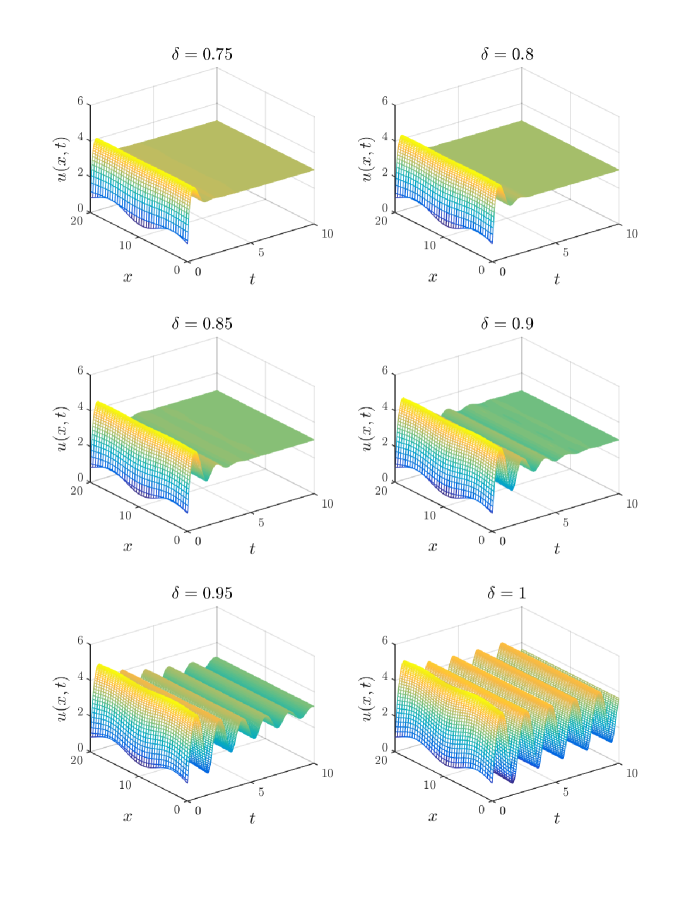
Figure 1: One dimensional concentration $u\left(x,t\right)$ as a solution of (3.1) with $\left(a,b,\sigma,d_{1},d_{2}\right)=\left(15,1,7,1,10\right)\,$, initial conditions (5.1), zero Nuemann boundaries, and different values for $\delta$.

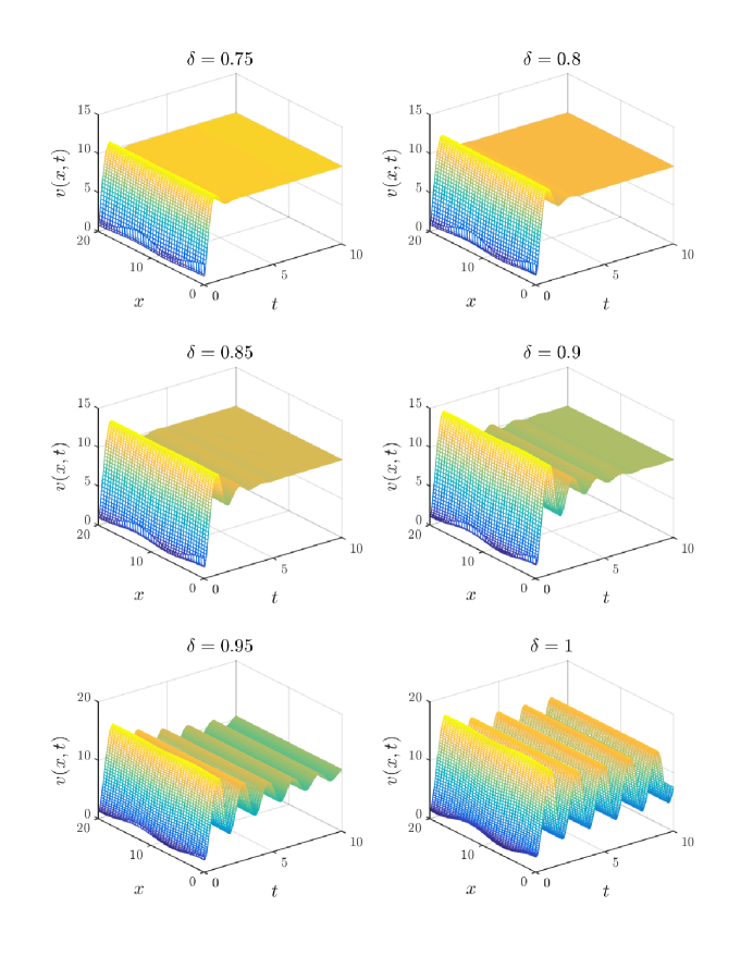
Figure 2: One dimensional concentration $v\left(x,t\right)$ as a solution of (3.1) with $\left(a,b,\sigma,d_{1},d_{2}\right)=\left(15,1,7,1,10\right)\,$, initial conditions (5.1), zero Nuemann boundaries, and different values for $\delta$.

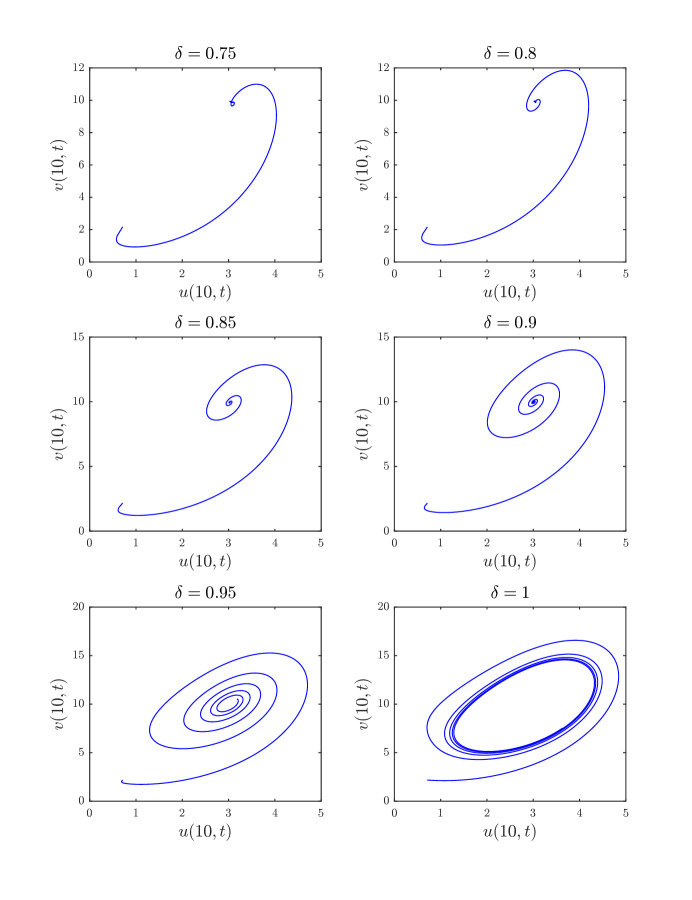
Figure 3: Phase plot of system (3.1) taken at $x=10$ with $\left(a,b,\sigma,d_{1},d_{2}\right)=\left(15,1,7,1,10\right)\,$, initial conditions (5.1), zero Nuemann boundaries, and different values for $\delta$.

In addition to these one–dimensional examples, we have also examined the two–dimensional case. We consider the parameter set $\left(a,b,\sigma,d_{1},d_{2}\right)=\left(15,1.2,8,1,24\right)$ with initial conditions

$$\left\{\begin{array}[]{l}u\left(x,y,0\right)=3.5\left(1+0.2w_{u}\left(x,y\right)\right),\vskip 6.0pt plus 2.0pt minus 2.0pt\\ v\left(x,y,0\right)=10.5\left(1+0.2w_{v}\left(x,y\right)\right).\end{array}\right.$$ (5.3)

with $w_{u}\left(x,y\right)$ and $w_{v}\left(x,y\right)$ being Gaussian distributed random functions with zero mean and unit variance. Figure 4 shows snap shots of the concentrations $u\left(x,y,t\right)$ and $v\left(x,y,t\right)$ taken at time instances $t=0$, $t=5$, and $t=20$ with $\delta=1$. We see that the diffusion–driven or Turing instability leads to the formation of patterns in the form of dots and stripes. Reducing the fractional order to $\delta=0.98$ leads to a different type of patterns as shown in Figure 5. This means that the fractional order has an impact on the Turing patterns evolving over time, which is an interesting observation. Reducing the fractional order further to $\delta=0.95$ also yields slightly different patterns as shown in Figure 6.

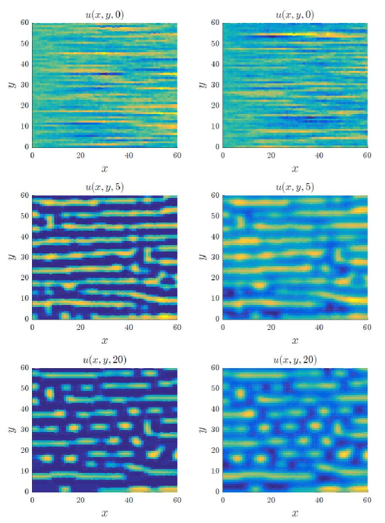
Figure 4: Two dimensional concentrations $u\left(x,y,t\right)$ and $v\left(x,y,t\right)$ for $\left(a,b,\sigma,d_{1},d_{2}\right)=\left(15,1.2,8,1,24\right)\,$, initial conditions (5.3), zero Nuemann boundaries, and $\delta=1$.

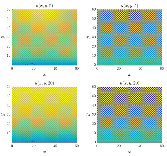
Figure 5: Two dimensional concentrations $u\left(x,y,t\right)$ and $v\left(x,y,t\right)$ for $\left(a,b,\sigma,d_{1},d_{2}\right)=\left(15,1.2,8,1,24\right)\,$, initial conditions (5.3), zero Nuemann boundaries, and $\delta=0.98$.

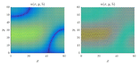
Figure 6: Two dimensional concentrations $u\left(x,y,t\right)$ and $v\left(x,y,t\right)$ for $\left(a,b,\sigma,d_{1},d_{2}\right)=\left(15,1.2,8,1,24\right)\,$, initial conditions (5.3), zero Nuemann boundaries, and $\delta=0.95$.

6 Concluding Remarks

In this paper, we have considered a time–fractional version of the Lengyel–Epstein system modeling the chlorite–iodide malonic acid (CIMA) chemical reaction. The Lengyel–Epstein model is well known for exhibiting Turing patterns, which makes it of interest to researchers in mathematics, chemistry, and biology. Introducing fractional time derivatives has recently been shown to model natural phenomena more accurately especially in chemical reactions. We have established sufficient conditions for the local asymptotic stability of the system’s unique equilibrium in the ODE and PDE senses through the linearization method. In addition, we have employed the direct Lyapunov method to establish the global asymptotic stability of the steady state solution.

Through numerical investigation, we have seen that a periodic solution in the standard case, which corresponds to pattern formation, became asymptotically stable when the differentiation order decreased below $1$. This is an important observation that requires closer investigation and analysis as it provides a new perspective into the control and applications of the Lengyel–Epstein system. We have also seen that the presence of diffusion alters the stability conditions of the system, which is not at all unlike the standard case. Furthermore, we saw that the type of patterns that form as a result of the diffusion–driven instability changes as the fractional order is varied. More investigation will be performed in future studies to explore these observations.

References

- [1] I. Lengyel, I. R. Epstein, A chemical approach to designing Turing patterns in reaction-diffusion system, Proc. Nat. Acad. Sci USA, 89 (1992) 3977-3979.
- [2] I. Lengyel, I. R. Epstein, Modeling of Turing structures in the chlorite–iodide–malonic acid–starch reaction system, Science, 251 (1991) 650-652.
- [3] P. DeKepper, I. R. Epstein, M. Orban, K. Kustin, Batch Oscillations and Spatial Wave Patterns in Chlorite Oscillating Systems, J. Phys. Chem., Vol. 86 (1982), pp. 170–171.
- [4] A.Turing, The chemical basis of morphogenesis, Philos.Trans. R. Soc. Lond. Ser. 237 (641)(1952) 37–72.
- [5] W. M. Ni, M. Tang, Turing patterns in the Lengyel–Epstein system for the CIMA reaction, Trans. Amer. Math. Soc. 357 (2005) 3953–3969.
- [6] F. Yi, J. Wei, J. Shi, Diffusion-driven instability and bifurcation in the Lengyel–Epstein system, Nonlinear Anal. RWA 9 (2008) 1038–1051.
- [7] F. Yi, J. Wei, J. Shi, Global asymptotic behavior of the Lengyel–Epstein reaction–diffusion system, Appl. Math. Lett. 22 (2009) 52–55.
- [8] B. Lisena, On the global dynamics of the Lengyel–Epstein system, Appl. Math. &Comp. 249, 67–75 (2014).
- [9] L. Wang, H. Zhao, Hopf bifurcation and Turing instability of 2–D Lengyel–Epstein system with reaction–diffusion terms, Appl. Math. Comput. 219 (2013) 9229–9244.
- [10] F.A. dos S. Silva, R.L. Viana, S.R. Lopes, Pattern formation and Turing instability in an activator–inhibitor system with power–law coupling, Physica A, Vol. 419 (2015), pp. 487–497.
- [11] J. Jang, W. Ni, M. Tang, Global bifurcation and structure of Turing patterns in the 1D Lengyel–Epstein model, J. Dyn. Diff. Eqs., Vol. 16(2) (2004), pp. 297–320.
- [12] A.K. Horvath, M. Dolnik, A.M. Zhabotinsky, I.R. Epstein, Kinetics of photoresponse of the chlorine dioxide-iodine-malonic acid reaction, J. Phys. Chem. A, Vol. 104(24) (2000), 5766.
- [13] S. Rudiger, D. G. Miguez, A. P. Munuzuri, F. Sagués, J. Casademunt, Dynamics of Turing patterns under spatiotemporal forcing, Phys. Rev. Lett., Vol. 90 (2003), 128301.
- [14] D.G. Miguez, S. Alonso, A.P. Munuzuri, F. Sagues, Experimental evidence of localized oscillations in the photosensitive chlorine dioxide-iodine-malonic acid reaction, Phys. Rev. Letters, Vol. 97 (2006), 178301.
- [15] D. Cuias-Vazquez, J. Carballido-Landeira, V. Pérez-Villar, A. P. Munuzuri1, Chaotic behaviour induced by modulated illumination in the Lengyel-Epstein model under Turing considerations, Chaotic Modeling and Simulation (CMSIM), Vol. 1 (2012), pp. 45–51.
- [16] C. Scholz, Morphology of experimental and simulated Turing patterns, Friedrich-Alexander-University, Germany, (2009).
- [17] J. Zheng, Time optimal controls of the Lengyel–Epstein model with internal control, Appl. Math. Optim., Vol. 70 (2014), pp. 345–371.
- [18] G. Gambino, M.C. Lombardo, M. Sammartino, Turing instability and pattern formation for the Lengyel–Epstein system with nonlinear diffusion, Acta. Appl. Math., Vol. 132 (2014), pp. 283–294.
- [19] J. Zheng, Optimal control problem for Lengyel–Epstein model with obstacles and state constraints, Nonlinear Analysis: Modelling and Control, Vol. 21(1) (2016), pp. 18–39.
- [20] X. Wei, J. Wei, Stability and bifurcation analysis in the photosensitive CDIMA system with delayed feedback control, Int. J. Bifurcation and Chaos, Vol. 27(11) (2017), 1750177.
- [21] S. Abdelmalek, S. Bendoukha, On the global asymptotic stability of solutions to a generalized Lengyel-Epstein system, Nonlinear Analysis: Real World Applications, Vol. 35 (2017), pp. 397-413.
- [22] S. Abdelmalek, S. Bendoukha, and B. Rebiai, On the stability and nonexistence of Turing patterns for the generalised Lengyel-Epstein model. Math Meth Appl Sci. 2017;1-11. https://doi.org/10.1002/mma.4457.
- [23] S. Abdelmalek, S. Bendoukha, B. Rebiai, M. Kirane, Extended Global Asymptotic Stability Conditions for a Generalized Reaction–Diffusion System, to appear in Acta Appl Math, Springer Nature B.V. 2018.
- [24] S. Abdelmalek, S. Bendoukha, M. Kirane, The global existence and asymptotic stability of solutions for a reaction-diffusion system, to appear.
- [25] B. Liu, R. Wu, N. Iqbal, Turing patterns in the Lengyel–Epstein system with superdiffusion, Int. J. Bifurcation and Chaos, Vol. 27(8) (2017), 1730026.
- [26] A. Kilbas, H. Srivastava, J. Trujillo, Theory and applications of fractional differential equations, Elsevier, (2006).
- [27] Y. Li, Y.Q. Chen, I. Podlubny, Stability of fractional-order nonlinear dynamic systems: Lyapunov direct method and generalized Mittag–Leffler stability, Computers & Mathematics with Applications, Vol. 59(5) (2010), pp. 1810–1821.
- [28] N. Aguila–Camacho, M.A. Duarte–Mermoud, J.A. Gallegos, Lyapunov functions for fractional order systems, Commun Nonlinear Sci Numer Simulat, Vol. 19 (2014), pp. 2951–2957.
- [29] D. Matignon, Stability results for fractional differential equations with applications to control processing, Proceedings of the IMACS–SMC, Vol. 2 (1996), pp. 963–968.
- [30] W. Deng, C, Li, J. Lu, Stability analysis of linear fractional differential system with multiple time delays, Nonlinear Dynamics, Vol. 48 (2007), pp. 409–416.
- [31] P. De Mottoni, F. Rothe, Convergence to homogeneous equilibrium state for generalized Volterra–Lotka systems with diffusion, SIAM J. Appl. Math., Vol. 37 (3) (1979) 648–663.
- [32] R. G. Casten, C. J. Holland, Stability properties of solutions to systems of reaction-diffusion equations, SIAM J. Appl. Math., Vol. 33 (1977), pp. 353–364.
- [33] A. Alsaedi, B. Ahmad, M. Kirane, Maximum principle for certain generalized time and space fractional diffusion equations, Quarterly of Applied Math, Vol. 73(1) (2015), pp. 163–175.
- [34] I. Podlubny, K. V. Thimann : Fractional Differential Equations.Series: Mathematics in science and engineering 198, Academic Press, San Diego, 1999