Two-field Cosmological $\alpha$-attractors with Noether Symmetry

Lilia Anguelova^a, Elena Mirela Babalic^b and Calin Iuliu Lazaroiu<sup>c

a</sup> Institute for Nuclear Research and Nuclear Energy, BAS, Sofia, Bulgaria
^b Horia Hulubei National Institute for Physics and Nuclear Engineering (IFIN-HH), Bucharest-Magurele, Romania
^c Center for Geometry and Physics, Institute for Basic Science, Pohang 37673, Republic of Korea

Abstract

We study Noether symmetries in two-field cosmological $\alpha$-attractors, investigating the case when the scalar manifold is an elementary hyperbolic surface. This encompasses and generalizes the case of the Poincaré disk. We solve the conditions for the existence of a ‘separated’ Noether symmetry and find the form of the scalar potential compatible with such, for any elementary hyperbolic surface. For this class of symmetries, we find that the $\alpha$-parameter must have a fixed value. Using those Noether symmetries, we also obtain many exact solutions of the equations of motion of these models, which were studied previously with numerical methods.

1 Introduction

A period of an accelerated expansion in the Early Universe is thought to be necessary for explaining the large-scale properties of the present day Universe. The standard description of such an inflationary stage is given by coupling the space-time metric to one or more fundamental scalars, which have a nontrivial potential that temporarily dominates the energy density of the Universe. There is, in fact, a wide variety of such inflationary models. A particular class, called $\alpha$-attractors [1, 2] (see also the earlier related works [3, 4]), stands out as being in an especially good agreement with the current observational data.

This class of models has certain universal predictions for the important cosmological observables $n_{s}$ (scalar spectral index) and $r$ (tensor-to-scalar ratio). It has been understood that the key reason for this is a specific property of the kinetic terms of the scalars. More precisely, they are characterized by hyperbolic geometry [5, 6]. In fact, the original works on $\alpha$-attractors focused mostly on effectively single field models. The widest generalization in the context of two-field models, which brings into sharp focus the essential role of the hyperbolic geometry of the scalar kinetic terms and of uniformization theory, was introduced in [14] and further explored in [15, 16] by considering models whose scalar manifolds are arbitrary hyperbolic surfaces, which can be much more complicated than the Poincaré disk.

Although single-field inflationary models are the most studied, it is quite natural to consider models with more than one scalar field. The reason is that the underlying particle physics descriptions, including string compactifications, usually contain many scalars. So it makes sense to expect, in the context of a fundamental theory of matter and gravity, that more than one field would play an important role during an inflationary stage. In view of very recent developments in the literature, there may also be another motivation to be interested in multi-field cosmological models. Namely, it was conjectured in [18] that quantum gravity requires the scalar potential to satisfy a certain condition, which excludes dS minima and seems to be in severe tension with single-field slow-roll inflationary models [19, 20]. It was argued in [21] that one can reconcile slow-roll inflation with the conjecture of [18] by considering multi-field models. One should note, however, that there are already serious objections [22, 23, 24, 25, 26] to that conjecture, whose only motivation is that it is rather difficult to find well-under-control stringy constructions that have (meta-)stable dS minima. It could be helpful, in sorting out arguments for or against the conjecture, to better understand multi-field inflationary models and their embeddings in string compactifications. Regardless of whether one is motivated by the conjecture of [18] or by the general expectation that more than one scalar field could play an important role for inflation, it is natural to be interested in two-field models as the simplest case of multi-field ones.

Most of the time, the equations of motion of two-field cosmological models are solved numerically in the literature. See, in particular, [15, 16, 17] for such numerical investigations in two-field $\alpha$-attractor models. Our goal here will be to find exact solutions by imposing the requirement that the model possesses a Noether symmetry. This method is well-known in the context of extended theories of gravity, where it has long been used to find classes of exact solutions [27, 28, 29, 30]. The basic idea is that the presence of a Noether symmetry constrains the form of an otherwise arbitrary function in the action (in our context, the scalar potential) and allows one to simplify the equations of motion. In general, this method does not give all solutions of the field equations, but only a certain subset. However, having exact solutions to analyze is often more informative conceptually than performing numerical analysis. Furthermore, the relevant Noether symmetry may have a deeper meaning, if the two-field models under consideration could be embedded in some fundamental particle physics setup, like a class of string theory compactifications.

The Noether symmetry method was already applied to one-field $\alpha$-attractor models of inflation in [31]. However, due to the limitation to a single scalar field, that analysis could not illustrate the essential role played by the hyperbolic geometry of the scalar manifold. Here we will apply the Noether symmetry method to the two-field generalized $\alpha$-attractors of [14, 15, 16]. A key feature of this class of models is that the scalar manifold is a hyperbolic surface. For a Riemannian 2-manifold, hyperbolicity amounts to the condition that the Gaussian curvature is constant and negative. In fact, it is inversely proportional to the $\alpha$-parameter of these models. We will focus on the simplest class of hyperbolic surfaces, called elementary, of which there are three types: the Poincaré disk, the hyperbolic punctured disk and the hyperbolic annuli (see, for example, [15]). Using a separation-of-variables Ansatz, we show that two-field $\alpha$-attractor models, with scalar manifold given by any elementary hyperbolic surface, have a ‘separated’ Noether symmetry for a certain form of the scalar potential. The existence of such a symmetry requires a different form of the scalar potential for each of the three types of elementary hyperbolic surface. The hyperbolic geometry of the scalar kinetic terms will play an essential role in this derivation.

It turns out that the special kind of Noether symmetry, which we find using the separation of variables Ansatz, not only selects a particular form of the scalar potential, but also fixes the value of the otherwise arbitrary $\alpha$-parameter. That a specific value of the $\alpha$-parameter is required for a separated Noether symmetry may seem unexpected. However, it is also very intriguing. Recall that it is not uncommon, especially in the context of string theory, to have particular points in a certain parameter space, where an (enhanced) symmetry occurs, although there is no such symmetry at generic points of that parameter space. It would be very interesting to understand whether this peculiar feature can help find specific embeddings of two-field $\alpha$-attractor models with a separated Noether symmetry in a more fundamental particle physics framework.

We also find many exact solutions of the equations of motion of two-field $\alpha$-attractor models, which admit a separated Noether symmetry. To achieve this, we transform the relevant Lagrangian to a new system of generalized coordinates, which is adapted to the Noether symmetry. We investigate each of the elementary hyperbolic surfaces in detail and find a variety of exact solutions of the field equations in each case.

The organization of the present paper is the following. In Section 2, we briefly review the action for the class of cosmological models known as generalized two-field $\alpha$-attractors. The two-dimensional scalar manifold of those models is a hyperbolic surface. We write down the action for each elementary hyperbolic surface, namely the Poincaré disk, the hyperbolic punctured disk and the hyperbolic annuli. In Section 3, we write the cosmologically relevant point-particle Lagrangian (the so-called ‘minisuperspace Lagrangian’) and impose the condition that it has a Noether symmetry. This leads to a coupled system of seven PDEs. Using a separation-of-variables Ansatz, we find solutions of that system for each elementary hyperbolic surface, in particular determining the form of the scalar potential which is compatible with the separated Noether symmetry. In Section 4, we find new generalized coordinates that are adapted to this Noether symmetry. In Sections 5, 6 and 7, we investigate the equations of motion of the two-field $\alpha$-attractor Lagrangian in the new coordinate system for the Poincaré disk, hyperbolic punctured disk and hyperbolic annuli respectively. We find many exact solutions in each of the three cases. Section 8 summarizes our results and briefly mentions some directions for further research. Appendix A recalls the basic definitions and properties of elementary hyperbolic surfaces (whose geometry is described in detail in reference [15]). Appendix B illustrates some of the new exact solutions.

2 Two-field cosmological $\alpha$-attractor models

Generalized two-field $\alpha$-attractors are a class of inflationary models obtained from Einstein gravity coupled to a non-linear sigma-model with two real scalar fields, whose target space (known as the scalar manifold) is a hyperbolic surface. This system is described by the action

$$S=\int d^{4}x\,\sqrt{-g}\left[\,\frac{R}{2}-\frac{1}{2}\,G_{IJ}(\phi)\,\partial\phi^{I}\partial\phi^{J}-V(\phi)\,\right]\,,$$ (2.1)

where $R$ is the scalar curvature of the 4d space-time metric $g_{\mu\nu}$, the fields $\phi^{I}$ with $I=1,2$ are two real scalars and the non-linear sigma-model metric $G_{IJ}(\phi)$ is a complete hyperbolic metric, i.e. a complete metric of constant negative Gaussian curvature $K$ . For brevity, we use the notation $\partial\phi^{I}\partial\phi^{J}\equiv g^{\mu\nu}\partial_{\mu}\phi^{I}\partial_{\nu}\phi^{J}$.

The simplest example is obtained by taking the scalar manifold to be the Poincaré disk $\mathbb{D}$. In this case, using polar coordinates on $\mathbb{D}$ and considering only radial trajectories, one recovers the original one-field $\alpha$-attractors of [1, 2]. It was understood in [5, 6] that the universal properties of the latter arise from the hyperbolic geometry of the Poincaré disk. Later, reference [14] considered a very wide generalization of the Poincaré disk models, obtained by taking the scalar manifold to be an arbitrary hyperbolic surface and showed that the universal properties of the original one-field $\alpha$-attractors persist under certain conditions. Specific examples of generalized two-field $\alpha$-attractors were explored in more detail in [15, 16, 17]. In particular, [15] studied $\alpha$-attractors whose scalar manifold is an elementary hyperbolic surface, i.e. the Poincaré disk, the punctured hyperbolic disk or a hyperbolic annulus. We briefly review their definitions and properties in Appendix A.

Our goal here will be to show that, for each of the elementary hyperbolic surfaces, the cosmological model obtained from the action (2.1) possesses a Noether symmetry for a certain value of the parameter $\alpha$ and a particular form of the scalar potential $V(\phi)$. To achieve this goal, it will be useful to rewrite (2.1) in the form:

$$S=\int\!d^{4}x\,\sqrt{-g}\left[\frac{R}{2}-\frac{1}{2}(\partial\varphi)^{2}-\frac{f(\varphi)}{2}(\partial\theta)^{2}-V(\varphi,\theta)\right]\,,$$ (2.2)

where now the two real scalars are $\varphi$ and $\theta$ and all the information about the hyperbolic geometry of the sigma-model metric is contained in the function $f(\varphi)$. Such a rewriting can be achieved for any metric $G_{IJ}$, which admits a $U(1)$ isometry parameterized by $\theta$ and so, in particular, for any of the elementary hyperbolic surfaces. Namely:

$\bullet$  Poincaré disk:

When $G_{IJ}$ is the metric on the hyperbolic disk 𝔻, the action (2.1) can be written as:

$$S_{\hbox{\mybbb D}}=\int\!d^{4}x\,\sqrt{-g}\left[\frac{R}{2}-3\alpha\frac{\partial Z\partial\bar{Z}}{(1-Z\bar{Z})^{2}}-V(Z)\right]\,,$$ (2.3)

in terms of a complex scalar $Z=\phi^{1}+i\phi^{2}$. Writing the latter as:

$$Z=\rho e^{i\theta}$$ (2.4)

and performing the field redefinition:

$$\rho=\tanh\!\left(\frac{\varphi}{\sqrt{6\alpha}}\right)\,,$$ (2.5)

we find that (2.3) acquires the form (2.2) with the following function $f(\varphi)$:

$$f_{\hbox{\mybbb D}}(\varphi)=\frac{3\alpha}{2}\sinh^{2}\!\left(\sqrt{\frac{2}{3\alpha}}\,\varphi\right)\,\,\,.$$ (2.6)

$\bullet$  Hyperbolic punctured disk:

For $G_{IJ}$ the metric on the hyperbolic punctured disk $\mathbb{D}^{*}$, the action (2.1) can be written as:

$$S_{\hbox{\mybbb D}^{*}}=\int\!d^{4}x\,\sqrt{-g}\left[\frac{R}{2}-\frac{\alpha}{(\rho\ln\rho)^{2}}\left\{(\partial\rho)^{2}+\rho^{2}(\partial\theta)^{2}\right\}-V(\rho,\theta)\right]\,.$$ (2.7)

Hence, the field redefinition:

$$\varphi=\sqrt{2\alpha}\,\ln(|\ln\!\rho|)$$ (2.8)

transforms it into (2.2), where now the function $f(\varphi)$ is:

$$f_{\hbox{\mybbb D}^{*}}(\varphi)=2\alpha\,\exp\!\left(-\sqrt{\frac{2}{\alpha}}\,\varphi\right)\,\,\,.$$ (2.9)

$\bullet$  Hyperbolic annulus:

When $G_{IJ}$ is the metric on a hyperbolic annulus ${\mathbb{A}}$, (2.1) acquires the form:

$$S_{\hbox{\mybbb A}}=\int\!d^{4}x\,\sqrt{-g}\left[\frac{R}{2}-\frac{\alpha C_{R}^{2}}{[\rho\cos(C_{R}\ln\!\rho)]^{2}}\left\{(\partial\rho)^{2}+\rho^{2}(\partial\theta)^{2}\right\}-V(\rho,\theta)\right]\,,$$ (2.10)

where $C_{R}\equiv\frac{\pi}{2\ln\!\hat{R}}$. This can be transformed to the expression in (2.2) by the redefinition:

$$\varphi=\sqrt{2\alpha}\,\ln\!\left[\frac{1+\sin(C_{R}\ln\!\rho\,)}{\cos(C_{R}\ln\!\rho\,)}\right]\,,$$ (2.11)

which leads to the following function $f(\varphi)$:

$$f_{\hbox{\mybbb A}}(\varphi)=2\alpha C_{R}^{2}\,\cosh^{2}\!\left(\frac{\varphi}{\sqrt{2\alpha}}\right)\,\,\,.$$ (2.12)

3 Noether symmetries in two-field $\alpha$-attractors

We now investigate under what conditions the action (2.2), namely:

$$S=\int\!d^{4}x\,\sqrt{-g}\left[\frac{R}{2}-\frac{1}{2}(\partial\varphi)^{2}-\frac{f(\varphi)}{2}(\partial\theta)^{2}-V(\varphi,\theta)\right]\,,$$ (3.1)

has a Noether symmetry. As usual, we will consider the following Ansatz for the four-dimensional inflationary metric:

$$ds_{4}^{2}=-dt^{2}+a^{2}(t)d\vec{x}^{2}\,,$$ (3.2)

as well as spatially-homogeneous scalar fields $\varphi(x^{\mu})=\varphi(t)$ and $\theta(x^{\mu})=\theta(t)$. Substituting these in (3.1), we obtain:

$$S=\int\!d^{4}x\,a^{3}\!\left[\frac{3(\dot{a}^{2}+a\ddot{a})}{a^{2}}+\frac{\dot{\varphi}^{2}}{2}+\frac{f(\varphi)}{2}\dot{\theta}^{2}-V(\varphi,\theta)\right]\,.$$ (3.3)

Note that, since here $a$, $\varphi$ and $\theta$ depend only on time, the action per unit spatial volume in (3.3) can be viewed as the classical action of a mechanical system with three degrees of freedom.

To use the Noether method, we have to rewrite the Lagrangian in (3.3) in canonical form, namely as ${\cal L}(q^{i},\dot{q}^{i})$ in terms of some generalized configuration space coordinates $q^{i}$ and the corresponding generalized velocities $\dot{q}^{i}$. To achieve this, we use integration by parts in the $\ddot{a}$ term in (3.3). This allows us to write the action per unit spatial volume in (3.3) as $\int\!dt\,{\cal L}$ , with the following Lagrangian density:

$${\cal L}=-3a\dot{a}^{2}+\frac{a^{3}\dot{\varphi}^{2}}{2}+\frac{a^{3}f(\varphi)\,\dot{\theta}^{2}}{2}-a^{3}V(\varphi,\theta)\,\,\,.$$ (3.4)

In this point-like Lagrangian, we can view $\{a,\varphi,\theta\}$ as generalized coordinates on the configuration space ${\cal M}=\mathbb{R}^{2}\times\mathrm{S}^{1}$. Then $\{a,\dot{a},\varphi,\dot{\varphi},\theta,\dot{\theta}\}$ provide coordinates on the corresponding tangent bundle $T{\cal M}$. Let us now write down the conditions for (3.4) to have a Noether symmetry.

3.1 The Noether system

Recall that a symmetry generator is a vector field $X$ defined on $T{\cal M}$, which preserves the Lagrangian:

$$L_{X}{\cal L}=0~{}~{},$$ (3.5)

where $L_{X}$ is the Lie derivative along $X$. In fact, to generate a Noether symmetry of ${\cal L}$, the vector field $X$ has to be of the specific form:

$$X=\lambda_{a}\frac{\partial}{\partial a}+\dot{\lambda}_{a}\frac{\partial}{\partial\dot{a}}+\lambda_{\varphi}\frac{\partial}{\partial\varphi}+\dot{\lambda}_{\varphi}\frac{\partial}{\partial\dot{\varphi}}+\lambda_{\theta}\frac{\partial}{\partial\theta}+\dot{\lambda}_{\theta}\frac{\partial}{\partial\dot{\theta}}\,\,\,\,,$$ (3.6)

where the coefficients $\lambda_{a,\varphi,\theta}$ are functions of the configuration space coordinates $\{a,\varphi,\theta\}$. Hence, the condition (3.5) becomes:

$$\lambda_{a}\frac{\partial{\cal L}}{\partial a}+\dot{\lambda}_{a}\frac{\partial{\cal L}}{\partial\dot{a}}+\lambda_{\varphi}\frac{\partial{\cal L}}{\partial\varphi}+\dot{\lambda}_{\varphi}\frac{\partial{\cal L}}{\partial\dot{\varphi}}+\lambda_{\theta}\frac{\partial{\cal L}}{\partial\theta}+\dot{\lambda}_{\theta}\frac{\partial{\cal L}}{\partial\dot{\theta}}=0\,\,\,.$$ (3.7)

Let us now investigate the implications of this condition for the Lagrangian (3.4). First, note that all terms in (3.7) are either quadratic in the generalized velocities $\dot{a}$, $\dot{\varphi}$ and $\dot{\theta}$ or contain no velocity at all. So we can view the left-hand side of (3.7) as a second degree polynomial in the generalized velocities. Since we want to find functions $\lambda_{a,\varphi,\theta}(a,\varphi,\theta)$ , for which the symmetry condition (3.7) is satisfied identically, we have to require that each coefficient of this polynomial vanishes separately. Therefore, computing the various terms in (3.7) for the Lagrangian (3.4), we find the following coupled system (where in brackets we indicate the corresponding coefficient of the velocity polynomial):

$${\rm(E1)}\qquad (\mathrm{coeff.~{}of}~{}\dot{a}^{2}) :\qquad\hskip 5.69046pt \lambda_{a}+2a\frac{\partial\lambda_{a}}{\partial a}=0\,\,,$$

$${\rm(E2)}\qquad (\mathrm{coeff.~{}of}~{}\dot{\varphi}^{2}) :\qquad\hskip 5.69046pt \frac{3}{2}\lambda_{a}+a\frac{\partial\lambda_{\varphi}}{\partial\varphi}=0\,\,,$$

$${\rm(E3)}\qquad (\mathrm{coeff.~{}of}~{}\dot{\theta}^{2}) :\qquad\hskip 5.69046pt \frac{3}{2}f(\varphi)\lambda_{a}+\frac{a}{2}(\partial_{\varphi}f)\lambda_{\varphi}+a\,f(\varphi)\frac{\partial\lambda_{\theta}}{\partial\theta}=0\,\,,$$

$${\rm(E4)}\qquad (\mathrm{coeff.~{}of}~{}\dot{a}\dot{\varphi}) :\qquad\hskip 5.69046pt -6\frac{\partial\lambda_{a}}{\partial\varphi}+a^{2}\frac{\partial\lambda_{\varphi}}{\partial a}=0\,\,,$$

$${\rm(E5)}\qquad (\mathrm{coeff.~{}of}~{}\dot{a}\dot{\theta}) :\qquad\hskip 5.69046pt -6\frac{\partial\lambda_{a}}{\partial\theta}+a^{2}f(\varphi)\frac{\partial\lambda_{\theta}}{\partial a}=0\,\,,$$

$${\rm(E6)}\qquad (\mathrm{coeff.~{}of}~{}\dot{\varphi}\dot{\theta}) :\qquad\hskip 5.69046pt \frac{\partial\lambda_{\varphi}}{\partial\theta}+f(\varphi)\frac{\partial\lambda_{\theta}}{\partial\varphi}=0\,\,,$$

$${\rm(E7)}\quad ({\rm ind.\,\,of\,\,velocity}) :\qquad\hskip 5.69046pt 3V\lambda_{a}+aV_{\varphi}\lambda_{\varphi}+aV_{\theta}\lambda_{\theta}=0\,\,.$$ (3.8)

In the next subsections, we will show that equations (E1)-(E6) can be solved for any function $f(\varphi)$, such that the scalar manifold metric in (3.1) is hyperbolic, i.e. with a constant negative Gaussian curvature. Then, equation (E7) determines a particular form of the scalar potential. As in [31], we will look for solutions with the following separation-of-variables Ansatze:

$$\lambda_{a}(a,\varphi,\theta) = A_{1}(a)\Phi_{1}(\varphi)\Theta_{1}(\theta)\quad,$$

$$\lambda_{\varphi}(a,\varphi,\theta) = A_{2}(a)\Phi_{2}(\varphi)\Theta_{2}(\theta)\quad,$$

$$\lambda_{\theta}(a,\varphi,\theta) = A_{3}(a)\Phi_{3}(\varphi)\Theta_{3}(\theta)\quad.$$ (3.9)

Let us begin by considering equations (E1), (E2) and (E4), which do not depend on $f(\varphi)$ and hence have the same form for any elementary hyperbolic surface.

3.2 Solving equations (E1), (E2) and (E4)

Substituting (3.1) in equation (E1), we obtain the following first order ODE:

$$A_{1}(a)+2a\frac{dA_{1}}{da}=0\,\,.$$ (3.10)

Its general solution is:

$$A_{1}(a)=\frac{A}{\sqrt{a}}\,\,,$$ (3.11)

where $A$ is an arbitrary integration constant.

Equating the expressions for $\lambda_{a}$ obtained from (E1) and (E2) in (3.1), we have:

$$\frac{\partial\lambda_{a}}{\partial a}=\frac{1}{3}\frac{\partial\lambda_{\varphi}}{\partial\varphi}\,\,.$$ (3.12)

Substituting (3.1) in (3.12), we find the following set of equations:

$$\frac{dA_{1}}{da}=\frac{A_{2}(a)}{3}\quad,\quad\Phi_{1}(\varphi)=k\frac{d\Phi_{2}}{d\varphi}\quad,\quad\Theta_{1}(\theta)=\frac{1}{k}\Theta_{2}(\theta)\,\,,$$ (3.13)

where $k=const$. Using (3.11) in the first equation of (3.13) gives:

$$A_{2}(a)=-\frac{3}{2}\frac{A}{a^{3/2}}\,\,.$$ (3.14)

Let us now consider equation (E4). Substituting (3.1), (3.11) and (3.14) in this equation gives:

$$-8\frac{d\Phi_{1}}{d\varphi}\Theta_{1}(\theta)+3\Phi_{2}(\varphi)\Theta_{2}(\theta)=0\,\,.$$ (3.15)

This, together with the last relation in (3.13), implies that:

$$\Phi_{2}=\frac{8}{3k}\frac{d\Phi_{1}}{d\varphi}$$ (3.16)

Using the second equation of (3.13) in (3.16), we end up with the following ODE:

$$\frac{d^{2}\Phi_{2}(\varphi)}{d\varphi^{2}}-\frac{3}{8}\,\Phi_{2}(\varphi)=0\,\,,$$ (3.17)

whose general solution is:

$$\Phi_{2}(\varphi)=b_{1}\sinh\!\left(\sqrt{\frac{3}{8}}\,\varphi\right)+b_{2}\cosh\!\left(\sqrt{\frac{3}{8}}\,\varphi\right)\,\,,$$ (3.18)

where $b_{1,2}=const$. Using this in (3.13), we find:

$$\Phi_{1}(\varphi)=k\sqrt{\frac{3}{8}}\left[b_{1}\cosh\!\left(\sqrt{\frac{3}{8}}\,\varphi\right)+b_{2}\sinh\!\left(\sqrt{\frac{3}{8}}\,\varphi\right)\right]\,\,.$$ (3.19)

Note that our results above for $A_{1}(a)$, $A_{2}(a)$, $\Phi_{1}(\varphi)$ and $\Phi_{2}(\varphi)$ are consistent with those of [31], except that $b_{1}$ was set to zero in that work.

3.3 Solving equations (E5) and (E6)

Now we turn to equations (E5) and (E6) of (3.1). We will see below that, for an arbitrary function $f(\varphi)$, the (E5)-(E6) system does not have a solution compatible with (3.19). However, recall that we are only interested in functions $f$, such that the sigma-model metric in (3.1), namely the metric $ds^{2}=d\varphi^{2}+f(\varphi)d\theta^{2}$, is hyperbolic. We will show now that, for any such $f(\varphi)$, equations (E5) and (E6) can be solved in a manner compatible with (3.19).

Let us begin by substituting (3.1) in (E5). This gives

$$\Theta_{3}(\theta)=c\frac{d\Theta_{1}}{d\theta}\qquad{\rm with}\qquad c=const$$ (3.20)

and

$$A_{1}(a)-\beta a^{2}\frac{dA_{3}}{da}=0\qquad{\rm with}\qquad\beta=const\,\,,$$ (3.21)

as well as an equation for $\Phi_{3}(\varphi)$ which we will write down shortly. Using (3.11) allows us to solve (3.21) as:

$$A_{3}(a)=-\frac{2}{3}\frac{A}{\beta a^{3/2}}\,\,,$$ (3.22)

where we have set an additive integration constant to zero in order to ensure that $\frac{d\Phi_{3}}{d\varphi}\neq 0$ and $\frac{d\Theta_{2}}{d\theta}\neq 0$. Upon using (3.20) and (3.22), equation (E5) reduces to the following algebraic relation:

$$\Phi_{3}(\varphi)=\frac{6\beta}{c}\frac{1}{f(\varphi)}\,\Phi_{1}(\varphi)\,\,\,.$$ (3.23)

Let us now consider equation (E6) of (3.1). Substituting (3.14) and (3.22), one finds that the $a$-dependence factors out of this equation. Then, using the third relation of (3.13) together with (3.16), equation (E6) reduces to:

$$\frac{d\Phi_{3}}{d\varphi}=-\frac{6\beta}{c}\frac{1}{f(\varphi)}\frac{d\Phi_{1}}{d\varphi}\,\,\,.$$ (3.24)

Comparing the last relation with (3.23), we conclude that

$$\frac{1}{\Phi_{3}}\frac{d\Phi_{3}}{d\varphi}=-\frac{1}{\Phi_{1}}\frac{d\Phi_{1}}{d\varphi}\,\,\,,$$ (3.25)

which implies:

$$\Phi_{3}(\varphi)=\frac{\Phi_{0}}{\Phi_{1}(\varphi)}\,\,\,,$$ (3.26)

where $\Phi_{0}=const$. Substituting (3.26) in (3.23), we obtain:

$$\Phi_{1}(\varphi)=\sqrt{\frac{c\,\Phi_{0}}{6\beta}}\,\sqrt{f(\varphi)}$$ (3.27)

and thus

$$\Phi_{3}(\varphi)=\sqrt{\frac{6\beta\Phi_{0}}{c}}\frac{1}{\sqrt{f(\varphi)}}\,\,\,.$$ (3.28)

Clearly, for arbitrary $f(\varphi)$, the expression in (3.27) is not compatible with the $\Phi_{1}(\varphi)$ solution found in (3.19). However, we are interested only in functions $f(\varphi)$, for which the scalar manifold metric in (3.1) is hyperbolic. In other words, we are only considering $f(\varphi)$ such that the Gaussian curvature $K$ of the metric $ds^{2}=d\varphi^{2}+f(\varphi)d\theta^{2}$ is constant and negative. This restricts the form of the function $f$. To see how, let us compute the Gaussian curvature in question:

$$K=-\frac{1}{4}\frac{(2ff^{\prime\prime}-f^{\prime 2})}{f^{2}}\,\,\,,$$ (3.29)

where $f^{\prime}\equiv\partial_{\varphi}f$. Imposing the condition that $K=const<0$ , we can view (3.29) as an ODE for $f(\varphi)$. Solving it, we obtain:

$$f(\varphi)=\left[C_{1}^{\varphi}\cosh\!\left(\sqrt{|K|}\,\varphi\right)+C_{2}^{\varphi}\sinh\!\left(\sqrt{|K|}\,\varphi\right)\right]^{2}\qquad{\rm with}\qquad C_{1,2}^{\varphi}=const\,\,\,.$$ (3.30)

Substituting (3.30) in (3.27), we find that the result has the same form as (3.19). To completely match the two expressions for $\Phi_{1}(\varphi)$, we have to take

$$|K|=\frac{3}{8}\,\,\,.$$ (3.31)

Note that this will restrict the value of the $\alpha$-parameter in each of the three cases with $f$ given by (2.6), (2.9) and (2.12), as we will see shortly.

Let us now compare in more detail the solution (3.27), with $f$ given by (3.30), to the expression in (3.19), for each elementary hyperbolic surface. The general form of $f$ in (3.30) reduces to the specific form, in each of the three cases listed in equations (2.6), (2.9) and (2.12), for the following respective choices of the integration constants:

$$f=f_{\hbox{\mybbb D}} : \hskip 15.6491ptC_{1}^{\varphi}=0 {\rm and} \left(C_{2}^{\varphi}\right)^{2}=\frac{3\alpha}{2}\quad,$$

$$f=f_{\hbox{\mybbb D}^{*}} : \left(C_{1}^{\varphi}\right)^{2}=2\alpha {\rm and} C_{2}^{\varphi}=-C_{1}^{\varphi}\quad,$$

$$f=f_{\hbox{\mybbb A}} : \left(C_{1}^{\varphi}\right)^{2}=2\alpha C_{R}^{2} {\rm and} C_{2}^{\varphi}=0\quad.$$ (3.32)

Substituting these three cases for $f(\varphi)$ in relation (3.27) and comparing with (3.19) gives the following conditions for the existence of a solution:

𝔻 $$:\qquad b_{1}=0 ,\qquad b_{2}=\frac{1}{k}\sqrt{\frac{2\alpha c\,\Phi_{0}}{3\beta}} ,\qquad\alpha=\frac{16}{9}\quad,$$

$$\hbox{\mybb D}^{*} :\qquad b_{1}=\frac{2}{3k}\sqrt{\frac{2\alpha c\Phi_{0}}{\beta}} ,\qquad b_{2}=-b_{1} ,\qquad\alpha=\frac{4}{3}\quad,$$

𝔸 $$:\qquad b_{1}=\frac{2C_{R}}{3k}\sqrt{\frac{2\alpha c\Phi_{0}}{\beta}} ,\qquad b_{2}=0 ,\qquad\alpha=\frac{4}{3}\quad.$$ (3.33)

To recapitulate, we have shown that, upon choosing integration constants satisfying the constraints (3.3), the solutions of equations (E5) and (E6) are compatible with those of (E1), (E2) and (E4). More explicitly, the solutions for the functions $\Phi_{1,2}(\varphi)$ in the three cases of interest have the form:

$$\hbox{\mybb D}: \Phi_{1}(\varphi)=kb_{2}\sqrt{\frac{3}{8}}\,\sinh\!\left(\sqrt{\frac{3}{8}}\,\varphi\right)\quad,\quad\Phi_{2}(\varphi)=b_{2}\cosh\!\left(\sqrt{\frac{3}{8}}\,\varphi\right)\,\,\,,$$

$$\hbox{\mybb D}^{*}: \Phi_{1}(\varphi)=kb_{1}\sqrt{\frac{3}{8}}\,\exp\!\left(-\sqrt{\frac{3}{8}}\,\varphi\right)\quad,\quad\Phi_{2}(\varphi)=-b_{1}\exp\!\left(-\sqrt{\frac{3}{8}}\,\varphi\right)\,\,\,,$$

$$\hbox{\mybb A}: \Phi_{1}(\varphi)=kb_{1}\sqrt{\frac{3}{8}}\,\cosh\!\left(\sqrt{\frac{3}{8}}\,\varphi\right)\quad,\quad\Phi_{2}(\varphi)=b_{1}\sinh\!\left(\sqrt{\frac{3}{8}}\,\varphi\right)\,\,\,,$$ (3.34)

while $\Phi_{3}(\varphi)$ is given by (3.26) in all three cases. Also, for any function $f$, the solutions for $A_{1,2,3}(a)$ are:

$$A_{1}(a)=\frac{A}{a^{1/2}}\,\,\,\quad,\,\,\,\quad A_{2}(a)=-\frac{3}{2}\frac{A}{a^{3/2}}\,\,\,\quad,\,\,\,\quad A_{3}(a)=-\frac{2}{3}\frac{A}{\beta a^{3/2}}\,\,\,\quad,$$ (3.35)

as can be seen in (3.11), (3.14) and (3.22).

3.4 Solving equation (E3)

Next, we consider equation (E3) of the system (3.1). Substituting the solutions for $A_{1,2,3}(a)$ given in (3.35), we find that the $a$-dependence drops out from (E3). Then, using the third relation in (3.13), as well as (3.16) and (3.20), we find that (E3) reduces to:

$$3\left[f(\varphi)\Phi_{1}(\varphi)-\frac{4}{3}f^{\prime}\Phi_{1}^{\prime}\right]\Theta_{1}(\theta)-8\Phi_{1}(\varphi)\Theta_{1}^{\prime\prime}(\theta)=0\,\,\,.$$ (3.36)

Substituting (3.27) in (3.36) gives:

$$\left(3f^{2}-2f^{\prime 2}\right)\Theta_{1}(\theta)-8f(\varphi)\Theta_{1}^{\prime\prime}(\theta)=0\,\,\,.$$ (3.37)

Since the form of $f(\varphi)$ is fixed for each elementary hyperbolic surface, equation (3.37) is an ODE for the function $\Theta_{1}(\theta)$. This ODE admits solutions if and only if the following condition is satisfied:

$$\frac{\Theta_{1}^{\prime\prime}(\theta)}{\Theta_{1}(\theta)}=\frac{3f^{2}-2f^{\prime 2}}{8f}=const\equiv q\,\,\,.$$ (3.38)

It is easy to check that the expression $\frac{3f^{2}-2f^{\prime 2}}{8f}$ is indeed constant in each of the three cases of interest, namely the Poincaré disk, the punctured hyperbolic disk and the hyperbolic annuli. More precisely, substituting $f$ respectively from (2.6), (2.9) and (2.12) gives:

$$q_{\hbox{\mybbb D}}=-1\qquad,\qquad q_{\hbox{\mybbb D}^{*}}=0\qquad,\qquad q_{\hbox{\mybbb A}}=C_{R}^{2}\quad.$$ (3.39)

In fact, one can show directly that $\frac{3f^{2}-2f^{\prime 2}}{8f}=const$ for any $f(\varphi)$ , such that the scalar manifold metric in (3.1) is hyperbolic. Namely, using the form of $f(\varphi)$ given in (3.30) with $|K|=\frac{3}{8}$ , we obtain:

$$\frac{3f^{2}-2f^{\prime 2}}{8f}=\frac{3}{8}\left[(C_{1}^{\varphi})^{2}-(C_{2}^{\varphi})^{2}\right]\,\,\,.$$ (3.40)

Let us now study equation in (3.38) for each of the three values of $q$ given in (3.39).

$\bullet$  Poincaré disk:

For $q=-1$, relation (3.38) gives:

$$\Theta_{1}^{\prime\prime}(\theta)+\Theta_{1}(\theta)=0\,\,\,,$$ (3.41)

with the obvious solution

$$\Theta_{1}(\theta)=C_{1}\sin\theta+C_{2}\cos\theta\,\,.$$ (3.42)

Then (3.13) implies:

$$\Theta_{2}(\theta)=k\left(C_{1}\sin\theta+C_{2}\cos\theta\right)\,\,,$$ (3.43)

whereas (3.20) gives:

$$\Theta_{3}(\theta)=c\left(C_{1}\cos\theta-C_{2}\sin\theta\right)\,\,.$$ (3.44)

$\bullet$  Hyperbolic punctured disk:

For $q=0$, equation (3.38) becomes:

$$\Theta_{1}^{\prime\prime}(\theta)=0\,\,\,,$$ (3.45)

whose solution can be written as:

$$\Theta_{1}(\theta)=C_{3}\theta+\theta_{0}\qquad{\rm with}\qquad C_{3},\theta_{0}=const\,\,\,.$$ (3.46)

Using (3.46) as well as (3.13) and (3.20), we find:

$$\Theta_{2}(\theta)=k\!\left(C_{3}\theta+\theta_{0}\right)\qquad{\rm and}\qquad\Theta_{3}(\theta)=c\,C_{3}\,\,\,.$$ (3.47)

$\bullet$  Hyperbolic annulus:

For $q=C_{R}^{2}$, equation (3.38) takes the form:

$$\Theta_{1}^{\prime\prime}(\theta)-C_{R}^{2}\,\Theta_{1}(\theta)=0\,\,\,,$$ (3.48)

which has the general solution

$$\Theta_{1}(\theta)=C_{4}\cosh(C_{R}\theta)+C_{5}\sinh(C_{R}\theta)\,\,\,.$$ (3.49)

Hence, (3.13) and (3.20) give:

$$\Theta_{2}(\theta) = k\left[C_{4}\cosh(C_{R}\theta)+C_{5}\sinh(C_{R}\theta)\right]\,\,\,,$$

$$\Theta_{3}(\theta) = c\,C_{R}\left[C_{4}\sinh(C_{R}\theta)+C_{5}\cosh(C_{R}\theta)\right]\,\,\,.$$ (3.50)

3.5 Solving equation (E7): the scalar potential

So far, we have found functions $\lambda_{a,\varphi,\theta}(a,\varphi,\theta)$ , which solve equations (E1)-(E6) of the Noether system (3.1). Now we will show that the last equation of that system, namely (E7), determines the scalar potential $V(\varphi,\theta)$, if the latter is assumed to have the separation of variables form:

$$V(\varphi,\theta)=\tilde{V}(\varphi)\hat{V}(\theta)\,\,\,.$$ (3.51)

We begin by substituting (3.1) and (3.51) into (E7). Then, using the solutions for $A_{1,2,3}(a)$ given in (3.35) as well as the last relation in (3.13) (namely $\Theta_{2}=k\Theta_{1}$), we find that (E7) reduces to:

$$3\left[\tilde{V}(\varphi)\Phi_{1}(\varphi)-\frac{k}{2}\tilde{V}^{\prime}(\varphi)\Phi_{2}(\varphi)\right]\hat{V}(\theta)\Theta_{1}(\theta)-\frac{2}{3\beta}\tilde{V}(\varphi)\Phi_{3}(\varphi)\hat{V}(\theta)\Theta_{3}(\theta)=0\,\,\,.$$ (3.52)

Note that here we have not used any particular form of the function $f$. Hence, for any $f(\varphi)$, and thus for any $\Phi_{1,2,3}(\varphi)$ and $\Theta_{1,2,3}(\theta)$, we have the pair of equations

$$\frac{3\left[\tilde{V}(\varphi)\Phi_{1}(\varphi)-\frac{k}{2}\tilde{V}^{\prime}(\varphi)\Phi_{2}(\varphi)\right]}{\frac{2}{3\beta}\tilde{V}(\varphi)\Phi_{3}(\varphi)}=p=\frac{\hat{V}^{\prime}(\theta)\,\Theta_{3}(\theta)}{\hat{V}(\theta)\,\Theta_{1}(\theta)}\,\,\,,$$ (3.53)

where $p=const$. Clearly, then, one has two separate equations for the two functions $\tilde{V}(\varphi)$ and $\hat{V}(\theta)$. Let us now study these two equations for each of the three types of elementary hyperbolic surface.

$\bullet$  Poincaré disk:

Substituting the 𝔻 expressions from (3.3) and (3.3) into (3.53), we find the following equation for $\tilde{V}(\varphi)$:

$$\frac{d\tilde{V}(\varphi)}{d\varphi}+\frac{\sqrt{\frac{3}{8}}\left[\frac{p}{c}-2\sinh^{2}\!\left(\sqrt{\frac{3}{8}}\,\varphi\right)\right]}{\sinh\!\left(\sqrt{\frac{3}{8}}\,\varphi\right)\cosh\!\left(\sqrt{\frac{3}{8}}\,\varphi\right)}\,\tilde{V}(\varphi)=0\,\,\,.$$ (3.54)

Its general solution has the form:

$$\tilde{V}(\varphi)=\tilde{V}_{0}\cosh^{2}\!\left(\sqrt{\frac{3}{8}}\,\varphi\right)\coth^{\frac{p}{c}}\!\left(\sqrt{\frac{3}{8}}\,\varphi\right)\,\,\,,$$ (3.55)

where $\tilde{V}_{0}$ is an integration constant.

Using (3.42) and (3.44) inside (3.53), we obtain:

$$\frac{d\hat{V}(\theta)}{d\theta}-\frac{p}{c}\frac{(C_{1}\sin\theta+C_{2}\cos\theta)}{(C_{1}\cos\theta-C_{2}\sin\theta)}\,\hat{V}(\theta)=0\,\,\,,$$ (3.56)

whose solution is:

$$\hat{V}(\theta)=\hat{V}_{0}\left[C_{1}\cos\theta-C_{2}\sin\theta\right]^{-\frac{p}{c}}$$ (3.57)

with $\hat{V}_{0}=const$.

Therefore, for the case of the hyperbolic disk, the form of the scalar potential, that is compatible with Noether’s symmetry, is:

$$V(\varphi,\theta)=V_{0}\cosh^{2}\!\left(\sqrt{\frac{3}{8}}\,\varphi\right)\coth^{\frac{p}{c}}\!\left(\sqrt{\frac{3}{8}}\,\varphi\right)\left[C_{1}\cos\theta-C_{2}\sin\theta\right]^{-\frac{p}{c}}\,\,\,,$$ (3.58)

where $V_{0}=const$. Note that this expression reduces to the single-field result of [31] for $p=0$. It is also worth pointing out that the $\theta$-dependence in (3.57) allows as a special case the particular form needed for natural inflation. Indeed, by taking $C_{2}=0$ and $\frac{p}{c}=-2$, we have $\hat{V}(\theta)=const\times\cos^{2}\!\theta$. In that regard, it may be interesting to make a connection to the recent considerations of [8] on realizing natural inflation in two-field attractor models.

$\bullet$  Hyperbolic punctured disk:

Using the $\hbox{\mybb D}^{*}$ expressions from (3.3) and (3.3) in (3.53), we have:

$$\frac{d\tilde{V}(\varphi)}{d\varphi}+\sqrt{\frac{3}{2}}\left(1-\frac{p}{2c}\,e^{\sqrt{\frac{3}{2}}\,\varphi}\right)\tilde{V}(\varphi)=0\,\,\,,$$ (3.59)

whose solution is:

$$\tilde{V}(\varphi)=\tilde{V}_{0}\,\exp\!\left(\!-\sqrt{\frac{3}{2}}\,\varphi+\frac{p}{2c}e^{\sqrt{\frac{3}{2}}\varphi}\right)\,\,\,.$$ (3.60)

Now, substituting the solutions for $\Theta_{1,3}$ from (3.46) and (3.47) inside (3.53), we end up with:

$$\frac{d\hat{V}(\theta)}{d\theta}-\frac{p}{c}\!\left(\theta+\frac{\theta_{0}}{C_{3}}\right)\!\hat{V}(\theta)=0\,\,\,.$$ (3.61)

The solution of the last equation is:

$$\hat{V}(\theta)=\hat{V}_{0}\exp\!\left[{\frac{p\,\theta}{c}\!\left(\frac{\theta}{2}+\frac{\theta_{0}}{C_{3}}\right)}\!\right]\,\,\,.$$ (3.62)

Note that $p=0$ again gives a result independent of $\theta$ and thus leads to an effectively single-field system. It may be interesting to investigate this special case further and to see whether or how it differs from the single-field system studied in [31] (which arises from taking $p=0$ for the Poincaré disk).

$\bullet$  Hyperbolic annulus:

Finally, from the 𝔸 expressions in (3.3) and (3.3), substituted in (3.53), we obtain:

$$\frac{d\tilde{V}(\varphi)}{d\varphi}+\frac{\sqrt{\frac{3}{8}}\left[\frac{p}{cC_{R}^{2}}-2\cosh^{2}\!\left(\sqrt{\frac{3}{8}}\,\varphi\right)\right]}{\sinh\!\left(\sqrt{\frac{3}{8}}\,\varphi\right)\cosh\!\left(\sqrt{\frac{3}{8}}\,\varphi\right)}\,\tilde{V}(\varphi)=0\,\,\,.$$ (3.63)

Hence, in this case the solution for $\tilde{V}$ is:

$$\tilde{V}(\varphi)=\tilde{V}_{0}\sinh^{2}\!\left(\sqrt{\frac{3}{8}}\,\varphi\right)\coth^{\frac{p}{cC_{R}^{2}}}\!\left(\sqrt{\frac{3}{8}}\,\varphi\right)\,\,\,.$$ (3.64)

Now substituting (3.49) and (3.4) in (3.53), one finds the following equation for $\hat{V}$:

$$\frac{d\hat{V}(\theta)}{d\theta}-\frac{p}{cC_{R}}\frac{\left[C_{4}\cosh(C_{R}\theta)+C_{5}\sinh(C_{R}\theta)\right]}{\left[C_{4}\sinh(C_{R}\theta)+C_{5}\cosh(C_{R}\theta)\right]}\,\hat{V}(\theta)=0\,\,\,,$$ (3.65)

whose solution is given by:

$$\hat{V}(\theta)=\hat{V}_{0}\left[C_{4}\sinh(C_{R}\theta)+C_{5}\cosh(C_{R}\theta)\right]^{\frac{p}{cC_{R}^{2}}}\,\,\,.$$ (3.66)

4 New variables: cyclic coordinate

In this section, we will look for a suitable coordinate transformation $(a,\varphi,\theta)\rightarrow(u,v,w)$, such that $w$ is the cyclic coordinate corresponding to the symmetry with generator $X$ that we found above. This will be very useful for finding analytical solutions of the $\alpha$-attractor equations of motion for the following reason. In the new variables the symmetry generator will have the form $X=\frac{\partial}{\partial w}$ and thus the condition $L_{X}{\cal L}=0$ will become:

$$\frac{\partial{\cal L}}{\partial w}=0\,\,\,.$$ (4.1)

This will simplify the relevant equations of motion significantly, as we will see below. Note that, due to (4.1), the Euler-Lagrange equation for $w$ becomes:

$$\frac{d}{dt}\,\frac{\partial{\cal L}}{\partial\dot{w}}=0\,\,\,,$$ (4.2)

which shows that the generalized momentum $p_{w}\equiv\frac{\partial{\cal L}}{\partial\dot{w}}$ is conserved.

To find such coordinates, we must solve the conditions $i_{X}\mathrm{d}u=0$ ,  $i_{X}\mathrm{d}v=0$  and  $i_{X}\mathrm{d}w=1$, which amount to the system:

$$\lambda_{a}\frac{\partial u}{\partial a}+\lambda_{\varphi}\frac{\partial u}{\partial\varphi}+\lambda_{\theta}\frac{\partial u}{\partial\theta}=0\,\,\,,$$

$$\lambda_{a}\frac{\partial v}{\partial a}+\lambda_{\varphi}\frac{\partial v}{\partial\varphi}+\lambda_{\theta}\frac{\partial v}{\partial\theta}=0\,\,\,,$$

$$\lambda_{a}\frac{\partial w}{\partial a}+\lambda_{\varphi}\frac{\partial w}{\partial\varphi}+\lambda_{\theta}\frac{\partial w}{\partial\theta}=1\,\,\,,$$ (4.3)

Since the first two equations in (4) are formally identical, the general solutions for $u(a,\varphi,\theta)$ and $v(a,\varphi,\theta)$ will have the same form. Ensuring different functions for $u$ and $v$ will be due to choosing different values for (some of) the constants that characterize this general form, as will become clear below.

4.1 Finding the coordinates $u$ and $v$

In this subsection we consider the first equation in (4), namely

$$\lambda_{a}\frac{\partial u}{\partial a}+\lambda_{\varphi}\frac{\partial u}{\partial\varphi}+\lambda_{\theta}\frac{\partial u}{\partial\theta}=0\,\,\,.$$ (4.4)

As already pointed out, this will enable us to find not only $u$, but $v$ as well.

We will look for solutions with the separation of variables Ansatz:

$$u(a,\varphi,\theta)=A_{u}(a)\Phi_{u}(\varphi)\Theta_{u}(\theta)\,\,\,.$$ (4.5)

Using (3.1), (4.5) and the last relation in (3.13) (i.e. $\Theta_{2}=k\Theta_{1}$), equation (4.4) reduces to:

$$\left[A_{1}\Phi_{1}A_{u}^{\prime}\Phi_{u}+kA_{2}\Phi_{2}A_{u}\Phi_{u}^{\prime}\right]\Theta_{1}\Theta_{u}=-A_{3}\Phi_{3}A_{u}\Phi_{u}\Theta_{3}\Theta_{u}^{\prime}\,\,\,.$$ (4.6)

Separating out the $\theta$-dependence gives:

$$\frac{\Theta_{3}(\theta)}{\Theta_{1}(\theta)\Theta_{u}(\theta)}\frac{d\Theta_{u}(\theta)}{d\theta}=c_{\theta}$$ (4.7)

and

$$A_{1}\Phi_{1}A_{u}^{\prime}\Phi_{u}+kA_{2}\Phi_{2}A_{u}\Phi_{u}^{\prime}+c_{\theta}A_{3}\Phi_{3}A_{u}\Phi_{u}=0$$ (4.8)

for some $c_{\theta}=const$. Now, substituting $A_{1,2,3}(a)$ from (3.35) in (4.8), we find that the $a$-dependence factors out provided that:

$$\frac{dA_{u}}{da}=c_{a}\frac{A_{u}(a)}{a}$$ (4.9)

for some $c_{a}=const$. The last equation is solved by:

$$A_{u}(a)=a^{c_{a}}\,\,\,,$$ (4.10)

where for convenience we have set the overall multiplicative integration constant to one.

Substituting (4.10) and (3.35) in (4.8) gives:

$$\frac{3}{2}k\Phi_{2}\frac{d\Phi_{u}(\varphi)}{d\varphi}+\left(\frac{2}{3}\frac{c_{\theta}}{\beta}\Phi_{3}-c_{a}\Phi_{1}\!\right)\!\Phi_{u}(\varphi)=0\,\,\,.$$ (4.11)

This equation has different coefficients for each elementary hyperbolic surface, since the functions $\Phi_{1,2,3}(\varphi)$ differ in each case (see equation (3.3)). Before specializing to the various cases, we can further simplify (4.11) by using the expressions (3.27)-(3.28) and (3.16) for $\Phi_{1,2,3}$ in terms of the function $f(\varphi)$. This allow us to bring (4.11) to the form:

$$\frac{d\Phi_{u}(\varphi)}{d\varphi}+\frac{\left[\frac{2c_{\theta}}{c}-\frac{c_{a}}{2}f(\varphi)\right]}{f^{\prime}(\varphi)}\,\Phi_{u}(\varphi)=0\,\,\,.$$ (4.12)

To recapitulate, the solution for $A_{u}(a)$ is independent of $f$ and is given by (4.10). On the other hand, the solutions for $\Phi_{u}(\varphi)$ and $\Theta_{u}(\theta)$ do depend on the form of the function $f$ and are determined by equations (4.7) and (4.12), respectively. Let us now find $\Phi_{u}$ and $\Theta_{u}$ for each type of elementary hyperbolic surface.

$\bullet$  Poincaré disk:

For $f(\varphi)$ given in (2.6) with $\alpha=\frac{16}{9}$ (see the corresponding row in (3.3)), we find that (4.12) acquires the form:

$$\frac{d\Phi_{u}(\varphi)}{d\varphi}+\frac{\sqrt{\frac{3}{8}}\left[\frac{c_{\theta}}{c}-\frac{2c_{a}}{3}\sinh^{2}\!\left(\sqrt{\frac{3}{8}}\,\varphi\right)\right]}{\sinh\!\left(\sqrt{\frac{3}{8}}\,\varphi\right)\cosh\!\left(\sqrt{\frac{3}{8}}\,\varphi\right)}\,\Phi_{u}(\varphi)=0\,\,\,.$$ (4.13)

This equation has the general solution:

$$\Phi_{u}(\varphi)=\left[\coth\!\left(\sqrt{\frac{3}{8}}\,\varphi\right)\right]^{\frac{c_{\theta}}{c}}\left[\cosh\!\left(\sqrt{\frac{3}{8}}\,\varphi\right)\right]^{\frac{2c_{a}}{3}}\,\,\,,$$ (4.14)

where we have again set the overall integration constant to one for convenience. Note that the single-field result for $\Phi_{u}(\varphi)$ in (4.14) is obtained by taking $c_{\theta}=0$. Then, setting $c_{a}=3$, we find from (4.14) and (4.10) the same particular solution for $u(a,\varphi)=A_{u}(a)\Phi_{u}(\varphi)$, as that in [31].

Now, substituting (3.42) and (3.44) in (4.7), we find:

$$\frac{d\Theta_{u}(\theta)}{d\theta}-\frac{c_{\theta}}{c}\frac{(C_{1}\sin\theta+C_{2}\cos\theta)}{(C_{1}\cos\theta-C_{2}\sin\theta)}\,\Theta_{u}(\theta)=0\,\,\,,$$ (4.15)

whose solution is:

$$\Theta_{u}(\theta)=\left(C_{1}\cos\theta-C_{2}\sin\theta\right)^{-\frac{c_{\theta}}{c}}$$ (4.16)

with the overall integration constant once again set to one.

$\bullet$  Hyperbolic punctured disk:

Taking $f(\varphi)$ as in (2.9) with $\alpha=\frac{4}{3}$ (in accordance with the $\hbox{\mybb D}^{*}$ row of (3.3)), equation (4.12) becomes:

$$\frac{d\Phi_{u}(\varphi)}{d\varphi}+\sqrt{\frac{3}{8}}\left[\frac{2c_{a}}{3}-\frac{c_{\theta}}{c}\exp\!\left(\sqrt{\frac{3}{2}}\,\varphi\right)\right]\!\Phi_{u}(\varphi)=0\,\,\,.$$ (4.17)

This ODE is solved by

$$\Phi_{u}(\varphi)=\exp\left[-\frac{c_{a}}{\sqrt{6}}\,\varphi+\frac{c_{\theta}}{2c}\,\exp\!\left(\sqrt{\frac{3}{2}}\,\varphi\right)\right]\,\,,$$ (4.18)

where again the overall integration constant has been set to one.

The solution of (4.7), after substituting (3.46) and (3.47), is given by:

$$\Theta_{u}(\theta)=\exp\!\left[{\frac{c_{\theta}\,\theta}{c}\!\left(\frac{\theta}{2}+\frac{\theta_{0}}{C_{3}}\right)}\!\right]\,\,\,,$$ (4.19)

where the overall integration constant was set to one.

$\bullet$  Hyperbolic annulus:

For $f(\varphi)$ given by (2.12) with $\alpha=\frac{4}{3}$ (as in the 𝔸 line of (3.3)), equation (4.12) becomes:

$$\frac{d\Phi_{u}(\varphi)}{d\varphi}+\frac{\sqrt{\frac{3}{8}}\left[\frac{c_{\theta}}{cC_{R}^{2}}-\frac{2c_{a}}{3}\cosh^{2}\!\left(\sqrt{\frac{3}{8}}\,\varphi\right)\right]}{\sinh\!\left(\sqrt{\frac{3}{8}}\,\varphi\right)\cosh\!\left(\sqrt{\frac{3}{8}}\,\varphi\right)}\,\Phi_{u}(\varphi)=0\,\,\,.$$ (4.20)

Hence, the solution in this case is

$$\Phi_{u}(\varphi)=\left[\coth\!\left(\sqrt{\frac{3}{8}}\,\varphi\right)\right]^{\frac{c_{\theta}}{cC_{R}^{2}}}\left[\,\sinh\!\left(\sqrt{\frac{3}{8}}\,\varphi\right)\right]^{\frac{2c_{a}}{3}}\,\,\,.$$ (4.21)

Finally, the solution of (4.7), after substituting (3.49) and (3.4), has the form:

$$\Theta_{u}(\theta)=\left[C_{4}\sinh(C_{R}\theta)+C_{5}\cosh(C_{R}\theta)\right]^{\frac{c_{\theta}}{cC_{R}^{2}}}\,\,\,.$$ (4.22)

Remark on the coordinate $v$:

So far, we have found a function $u(a,\varphi,\theta)=A_{u}(a)\Phi_{u}(\varphi)\Theta_{u}(\theta)$, for each of the three cases under consideration, that solves the first equation in (4). As mentioned above, the second equation in (4) is then solved by a function $v(a,\varphi,\theta)=A_{v}(a)\Phi_{v}(\varphi)\Theta_{v}(\theta)$, such that $A_{v}$, $\Phi_{v}$ and $\Theta_{v}$ have the same general form as their $u$-indexed counterparts. To ensure that $v$ is a different function, one has to choose different values of the constants $c_{a}$ and $c_{\theta}$ than those taken for the function $u$.

4.2 Finding the cyclic coordinate $w$

Now we will consider the last equation in (4), namely:

$$\lambda_{a}\frac{\partial w}{\partial a}+\lambda_{\varphi}\frac{\partial w}{\partial\varphi}+\lambda_{\theta}\frac{\partial w}{\partial\theta}=1\,\,\,.$$ (4.23)

As usual, we will make the separation of variables Ansatz:

$$w(a,\varphi,\theta)=A_{w}(a)\Phi_{w}(\varphi)\Theta_{w}(\theta)\,\,\,.$$ (4.24)

Substituting (4.24), (3.1) and (3.35) in (4.23), it is easy to realize that the $a$-dependence can be canceled within each term by taking

$$A_{w}(a)=\frac{1}{A}\,a^{3/2}\,\,\,.$$ (4.25)

Using (4.25) and the relation $\Theta_{2}=k\Theta_{1}$ (see (3.13)), we find that (4.23) acquires the form:

$$\frac{3}{2}\left[\Phi_{1}\Phi_{w}-k\Phi_{2}\Phi_{w}^{\prime}\right]\Theta_{1}\Theta_{w}-\frac{2}{3\beta}\Phi_{3}\Phi_{w}\Theta_{3}\Theta_{w}^{\prime}=1\,\,\,.$$ (4.26)

Now we will show that one can remove the $\varphi$-dependence in (4.26) by a suitable choice of the function $\Phi_{w}(\varphi)$. The result will be an equation for $\Theta_{w}(\theta)$. Indeed, let us take:

$$\Phi_{w}(\varphi)=\frac{\phi_{0}}{\Phi_{3}(\varphi)}\qquad{\rm with}\qquad\phi_{0}=const\,\,\,.$$ (4.27)

Then, obviously, the second term in (4.26) becomes independent of $\varphi$. In addition, one can show that the combination $[\Phi_{1}\Phi_{w}-k\Phi_{2}\Phi_{w}^{\prime}]$ in the first term, with $\Phi_{w}$ given by (4.27), is a constant for each of the three cases in (3.3). In fact, one can see directly that this combination is constant for any function $f(\varphi)$ compatible with the hyperbolic geometry of the scalar manifold. Indeed, using (3.16), (4.27), (3.26) and (3.27), we obtain:

$$\Phi_{1}\Phi_{w}-k\Phi_{2}\Phi_{w}^{\prime}=\frac{\phi_{0}}{\Phi_{0}}\left[\Phi_{1}^{2}-\frac{8}{3}\,\Phi_{1}^{\prime 2}\right]=\frac{\phi_{0}c}{6\beta}\,\frac{\left(f^{2}-\frac{2}{3}f^{\prime 2}\right)}{f}\,\,\,.$$ (4.28)

Now recall relation (3.40), which holds for any $f(\varphi)$ of the form (3.30) with $|K|=\frac{3}{8}$. Using this relation, we find that (4.28) implies:

$$\Phi_{1}\Phi_{w}-k\Phi_{2}\Phi_{w}^{\prime}=\frac{\phi_{0}c}{6\beta}\left[\left(C_{1}^{\varphi}\right)^{2}-\left(C_{2}^{\varphi}\right)^{2}\right]=\frac{4}{9}\frac{\phi_{0}c}{\beta}q\,\,\,,$$ (4.29)

where for convenience we also wrote the result in terms of the constant $q$ defined in (3.38).

We are finally ready to extract an ODE for $\Theta_{w}(\theta)$. Substituting (4.27) and (4.29) into (4.26) gives:

$$\frac{2}{3}\frac{\phi_{0}}{\beta}\big{[}c\,q\,\Theta_{1}(\theta)\,\Theta_{w}(\theta)-\Theta_{3}(\theta)\,\Theta_{w}^{\prime}(\theta)\big{]}=1\,\,\,.$$ (4.30)

Then, using (3.20) and setting

$$\phi_{0}=-\frac{3}{2}\frac{\beta}{c}$$ (4.31)

in order to simplify the equation, we obtain from (4.30):

$$\Theta_{1}^{\prime}(\theta)\,\Theta_{w}^{\prime}(\theta)-q\,\Theta_{1}(\theta)\,\Theta_{w}(\theta)-1=0\,\,\,.$$ (4.32)

Let us now solve the last equation for each type of elementary hyperbolic surface.

$\bullet$  Poincaré disk:

In this case $q=-1$ (see (3.39)) and $\Theta_{1}(\theta)$ is given by (3.42). Therefore, (4.32) becomes:

$$\left[C_{1}\cos\theta-C_{2}\sin\theta\right]\frac{d\Theta_{w}}{d\theta}+\left[C_{1}\sin\theta+C_{2}\cos\theta\right]\Theta_{w}(\theta)-1=0\,\,\,.$$ (4.33)

The general solution of the last equation can be written as:

$$\Theta_{w}(\theta)=\frac{\sin\theta}{C_{1}}+\hat{C}_{\theta}\left[C_{1}\cos\theta-C_{2}\sin\theta\right]\qquad{\rm with}\qquad\hat{C}_{\theta}=const\,\,\,.$$ (4.34)

Note that, upon redefinition of the integration constant $\hat{C}_{\theta}$, the solution can also be written as:

$$\Theta_{w}(\theta)=\frac{\cos\theta}{C_{2}}+\hat{C}_{\theta}\left[C_{1}\cos\theta-C_{2}\sin\theta\right]$$ (4.35)

or as:

$$\Theta_{w}(\theta)=\frac{1}{2}\left(\frac{\sin\theta}{C_{1}}+\frac{\cos\theta}{C_{2}}\right)+\hat{C}_{\theta}\left[C_{1}\cos\theta-C_{2}\sin\theta\right]\,\,\,.$$ (4.36)

The last form might seem preferable, since it is symmetric with respect to interchange of the trigonometric functions sin and cos. However, this form requires both $C_{1}\neq 0$ and $C_{2}\neq 0$. On the other hand, the forms (4.34) and (4.35) allow one to take respectively the limits $C_{2}=0$ and $C_{1}=0$. Since we will be particularly interested in the limit $C_{2}=0$, we will use the form (4.34) in what follows (although we will comment more on using (4.36) below).

$\bullet$  Hyperbolic punctured disk:

In this case $q=0$ (see (3.39)). Also, $\Theta_{1}(\theta)$ has the form (3.46). Substituting these in (4.32), we obtain the ODE:

$$C_{3}\,\Theta_{w}^{\prime}(\theta)-1=0\,\,\,,$$ (4.37)

which has the solution:

$$\Theta_{w}(\theta)=\frac{\theta}{C_{3}}+const\,\,\,.$$ (4.38)

$\bullet$  Hyperbolic annulus:

In this case, relation (3.39) gives $q=C_{R}^{2}$ . Using this and the relevant $\Theta_{1}(\theta)$ expression (3.49), we find that (4.32) acquires the form:

$$C_{R}\big{[}C_{4}\sinh(C_{R}\theta)+C_{5}\cosh(C_{R}\theta)\big{]}\Theta_{w}^{\prime}(\theta)-C_{R}^{2}\big{[}C_{4}\cosh(C_{R}\theta)+C_{5}\sinh(C_{R}\theta)\big{]}\Theta_{w}(\theta)=1\,\,\,.$$ (4.39)

Similarly to the 𝔻 case above, the general solution of (4.39) can be written in three equivalent ways, namely:

$$\Theta_{w}(\theta)=\frac{\sinh(C_{R}\theta)}{C_{R}^{2}C_{5}}+\tilde{C}_{\theta}\big{[}C_{4}\sinh(C_{R}\theta)+C_{5}\cosh(C_{R}\theta)\big{]}$$ (4.40)

or

$$\Theta_{w}(\theta)=-\frac{\cosh(C_{R}\theta)}{C_{R}^{2}C_{4}}+\tilde{C}_{\theta}\big{[}C_{4}\sinh(C_{R}\theta)+C_{5}\cosh(C_{R}\theta)\big{]}$$ (4.41)

or

$$\Theta_{w}(\theta)=\frac{1}{2C_{R}^{2}}\left(\frac{\sinh(C_{R}\theta)}{C_{5}}-\frac{\cosh(C_{R}\theta)}{C_{4}}\right)+\tilde{C}_{\theta}\big{[}C_{4}\sinh(C_{R}\theta)+C_{5}\cosh(C_{R}\theta)\big{]}\,\,\,.$$ (4.42)

5 Equations of motion for the Poincaré disk

In this section our goal will be to find solutions to the equations of motion of the Lagrangian (3.4) for the case of the Poincaré disk. For that purpose, we will first rewrite the Lagrangian in terms of the new coordinates $(u,v,w)$ with the cyclic variable $w$. As already pointed out, this will lead to a significant simplification of the equations that will enable us to find analytical solutions.

Let us begin by summarizing the relevant results, which we have obtained so far for the two-field cosmological model based on the Poincaré disk. For $f(\varphi)$ given by (2.6) with $\alpha=\frac{16}{9}$ as in (3.3), the Lagrangian (3.4) has the form:

$${\cal L}=-3a\dot{a}^{2}+\frac{a^{3}\dot{\varphi}^{2}}{2}+\frac{4}{3}\,a^{3}\sinh^{2}\!\left(\sqrt{\frac{3}{8}}\,\varphi\right)\!\dot{\theta}^{2}-a^{3}V(\varphi,\theta)\,\,\,.$$ (5.1)

We found that (5.1) has a certain Noether symmetry, when the scalar potential is of the form (3.58), namely:

$$V(\varphi,\theta)=V_{0}\cosh^{2}\!\left(\sqrt{\frac{3}{8}}\,\varphi\right)\coth^{\frac{p}{c}}\!\left(\sqrt{\frac{3}{8}}\,\varphi\right)\left[C_{1}\cos\theta-C_{2}\sin\theta\right]^{-\frac{p}{c}}\,\,\,.$$ (5.2)

Also, according to (4.10), (4.14), (4.16), (4.25), (4.27) and (4.34), the general form of the new variables $u$, $v$ and $w$, with the latter being the cyclic coordinate corresponding to the Noether symmetry of Section 3, is the following:

$$u(a,\varphi,\theta) = a^{c_{a}^{u}}\left[\cosh\!\left(\sqrt{\frac{3}{8}}\,\varphi\right)\right]^{\frac{2c_{a}^{u}}{3}}\left[\coth\!\left(\sqrt{\frac{3}{8}}\,\varphi\right)\right]^{\frac{c_{\theta}^{u}}{c}}\left(C_{1}\cos\theta-C_{2}\sin\theta\right)^{-\frac{c^{u}_{\theta}}{c}}$$

$$v(a,\varphi,\theta) = a^{c_{a}^{v}}\left[\cosh\!\left(\sqrt{\frac{3}{8}}\,\varphi\right)\right]^{\frac{2c_{a}^{v}}{3}}\left[\coth\!\left(\sqrt{\frac{3}{8}}\,\varphi\right)\right]^{\frac{c_{\theta}^{v}}{c}}\left(C_{1}\cos\theta-C_{2}\sin\theta\right)^{-\frac{c^{v}_{\theta}}{c}}$$

$$w(a,\varphi,\theta) = C_{w}\,a^{3/2}\,\sinh\!\left(\sqrt{\frac{3}{8}}\,\varphi\right)\sin\theta\,\,\,,$$ (5.3)

where for convenience we have denoted $C_{w}\equiv-\frac{1}{AC_{1}}\sqrt{\frac{\beta}{c\,\Phi_{0}}}$ and have taken $\hat{C}_{\theta}=0$ in (4.34). Note that, to obtain this expression for the coefficient $C_{w}$ , one has to take into account (4.31), as well as the relevant coefficient for $\Phi_{1}(\varphi)$ according to (3.3)-(3.3). Finally, we have labeled the $c_{a}$ and $c_{\theta}$ constants, characterizing the functions $u(a,\varphi,\theta)$ and $v(a,\varphi,\theta)$ , with upper $u$ and $v$ indices, respectively, to underline the fact that their values in the two cases are independent of each other.

Now we are ready to rewrite the Lagrangian in terms of the variables $(u,v,w)$ and to study the resulting equations of motion. An important remark is in order, though, before we embark on that investigation. Namely, the Lagrangian (5.1) is subject to the Hamiltonian constraint $E_{\cal L}=0$, where

$$E_{\cal L}=\frac{\partial{\cal L}}{\partial\dot{q}^{i}}\,\dot{q}^{i}-{\cal L}$$ (5.4)

is the energy function corresponding to any point particle Lagrangian ${\cal L}(q^{i},\dot{q}^{i})$ with generalized coordinates $q^{i}$. It is well-known that the Hamiltonian $E_{\cal L}$ is conserved on any solutions of the Euler-Lagrange equations, i.e. that for such solutions one has $E_{\cal L}=const$. So imposing the constraint $E_{\cal L}=0$ (which is equivalent to the first order Einstein equation, often also called Friedman constraint) only results in a relation between the integration constants of the Euler-Lagrange equations; see for example [27]. Instead of just using the Hamiltonian constraint at the end of the computation, in order to eliminate one of the integration constants, it is tempting to try to utilize it from the start, in order to facilitate the search for solutions. However, since this constraint is generally (highly) non-linear, there is no guarantee that it will make a crucial difference for that purpose. In particular, for the cases that we will investigate below, it will turn out not to be useful in our search for analytical solutions.

5.1 Lagrangian in the new variables

To obtain the Lagrangian in terms of the new variables $u$, $v$ and $w$, we only need a particular coordinate transformation $(a,\varphi,\theta)\rightarrow(u,v,w)$. Hence, we can choose convenient values for the arbitrary constants $c_{a}^{u,v}$ and $c_{\theta}^{u,v}$ in (5). Particularly simple (and convenient for comparison with [31]) expressions are obtained for the following choices:

$$c^{u}_{\theta}=0\quad,\quad c^{u}_{a}=3\qquad\,\,\,{\rm and}\qquad\,\,\,c^{v}_{\theta}=-c\,\quad,\quad c^{v}_{a}=\frac{3}{2}\qquad.$$ (5.5)

Substituting (5.5) in (5) gives:

$$u = a^{3}\,\cosh^{2}\!\left(\sqrt{\frac{3}{8}}\,\varphi\right)\,\,\,,$$

$$v = a^{3/2}\,\sinh\!\left(\sqrt{\frac{3}{8}}\,\varphi\right)(C_{1}\cos\theta-C_{2}\sin\theta)\,\,\,\,,$$

$$w = C_{w}\,a^{3/2}\,\sinh\!\left(\sqrt{\frac{3}{8}}\,\varphi\right)\sin\theta\,\,\,\,.$$ (5.6)

Note that here we need $C_{1}\neq 0$, to ensure that $v$ and $w$ are independent variables. However, this was already tacitly assumed when using the $\Theta_{w}(\theta)$ solution (4.34) in (5); to allow for $C_{1}=0$, one would have to use the form (4.35) instead.

From now on, we will work with the coordinate transformation (5.1), whose inverse transformation is:

$$a = \left\{u-\left[\frac{1}{C_{1}^{2}}\left(\frac{v}{w}+\frac{C_{2}}{C_{w}}\right)^{2}+\frac{1}{C_{w}^{2}}\right]\!w^{2}\right\}^{1/3}\,\,\,,$$

$$\varphi = 2\sqrt{\frac{2}{3}}\,{\rm arccoth}\!\left(\sqrt{\frac{u}{w^{2}}}\left[\frac{1}{C_{1}^{2}}\left(\frac{v}{w}+\frac{C_{2}}{C_{w}}\right)^{2}+\frac{1}{C_{w}^{2}}\right]^{-1/2}\right)\,\,\,,$$

$$\theta = {\rm arccot}\!\left[\frac{C_{w}}{C_{1}}\!\left(\frac{v}{w}+\frac{C_{2}}{C_{w}}\right)\right]\,\,\,.$$ (5.7)

Note that, when $\theta=const$ , the variables $v$ and $w$ coincide up to a constant and the resulting expressions in (5.1) and (5.1) are consistent with the single-field ones obtained in [31].

Now, substituting (5.1) in (5.1)-(5.2), we find that in the new variables the Lagrangian is:

$${\cal L}=-\frac{1}{3}\frac{\dot{u}^{2}}{u}+\frac{4}{3}\frac{1}{C_{1}^{2}}\,\dot{v}^{2}+\frac{4}{3}\frac{1}{C_{w}^{2}}\left(1+\frac{C_{2}^{2}}{C_{1}^{2}}\right)\dot{w}^{2}+\frac{8}{3}\frac{C_{2}}{C_{1}^{2}C_{w}}\,\dot{v}\dot{w}-V_{0}\frac{u^{\frac{p}{2c}+1}}{v^{\frac{p}{c}}}\,\,\,.$$ (5.8)

As already mentioned above, the single-field case is obtained for $w=const\times v$ and $p=0$. In that case, the Lagrangian (5.8) is consistent with that in [31]. Also, note that the mixed term drops out for $C_{2}=0$, which is exactly the special case relevant for natural inflation as mentioned below (3.58).

Before we begin looking for solutions, let us underline again that (5.8) is subject to the Hamiltonian constraint $E_{\cal L}=0$, where

$$E_{\cal L}=\frac{\partial{\cal L}}{\partial\dot{u}}\,\dot{u}+\frac{\partial{\cal L}}{\partial\dot{v}}\,\dot{v}+\frac{\partial{\cal L}}{\partial\dot{w}}\,\dot{w}-{\cal L}\,\,\,,$$ (5.11)

as discussed above.

5.2 Solutions

It is convenient to introduce the notation:

$$m\equiv\frac{p}{c}\,\,\,.$$ (5.12)

Then the Euler-Lagrange equations of (5.8) are:

$$\left(1+\frac{C_{2}^{2}}{C_{1}^{2}}\right)\ddot{w}+\frac{C_{2}C_{w}}{C_{1}^{2}}\,\ddot{v} = 0\,\,\,,$$

$$V_{0}\,m\,\frac{u^{\frac{m}{2}+1}}{v^{m+1}}-\frac{8}{3}\left(\frac{1}{C_{1}^{2}}\,\ddot{v}+\frac{C_{2}}{C_{1}^{2}C_{w}}\,\ddot{w}\right) = 0\,\,\ ,$$

$$2u\ddot{u}-\dot{u}^{2}-3V_{0}\left(\frac{m}{2}+1\right)\frac{u^{\frac{m}{2}+2}}{v^{m}} = 0\,\,\,.$$ (5.13)

Note that in the single-field limit, which for us is given by $p=0$ (equivalently, $m=0$) and $v=const\times w$, this system is in complete agreement with [31].

To simplify the system (5.2), let us express $\ddot{w}$ from the first equation, namely

$$\ddot{w}=-\frac{C_{2}C_{w}}{C_{1}^{2}+C_{2}^{2}}\,\ddot{v}\,\,\,,$$ (5.14)

and introduce the function

$$\tilde{u}(t)\equiv\sqrt{u(t)}\,\,\,.$$ (5.15)

Substituting (5.14) and (5.15) in the second and third equations of (5.2) gives:

$$\ddot{v}-\frac{3}{8}V_{0}C_{0}\,m\,\frac{\tilde{u}^{m+2}}{v^{m+1}} = 0\,\,\,,$$

$$\ddot{\tilde{u}}-\frac{3}{8}V_{0}(m+2)\frac{\tilde{u}^{m+1}}{v^{m}} = 0\,\,\,,$$ (5.16)

where for convenience we have denoted $C_{0}\equiv C_{1}^{2}+C_{2}^{2}$.

Before we begin solving (5.2), let us make an important remark. Equation (5.14) can be solved immediately for $w$ in terms of $v$. One of the integration constants in this solution is determined by the constant of motion $\Sigma_{0}$, that is due to the Noether symmetry. Indeed, in general, $\Sigma_{0}$ is given by:

$$\Sigma_{0}\equiv\frac{\partial{\cal L}}{\partial\dot{w}}=\frac{8}{3}\frac{1}{C_{w}^{2}}\left(1+\frac{C_{2}^{2}}{C_{1}^{2}}\right)\dot{w}+\frac{8}{3}\frac{C_{2}}{C_{1}^{2}C_{w}}\,\dot{v}\,\,\,.$$ (5.17)

The first equation in (5.2) (equivalently, equation (5.14)) is precisely the time derivative of (5.17), due to the fact that $w$ is a cyclic coordinate. So the general solution for $w$ is:

$$w(t)=-\frac{C_{2}C_{w}}{(C_{1}^{2}+C_{2}^{2})}\,v(t)+\hat{\Sigma}_{0}\,t+C_{0}^{w}\,\,\,,$$ (5.18)

where $\hat{\Sigma}_{0}=\frac{3}{8}\frac{C_{1}^{2}C_{w}^{2}}{(C_{1}^{2}+C_{2}^{2})}\Sigma_{0}$ and $C_{0}^{w}=const$ . Hence, using (5.18) and (5.15) in (5.11), we have:

$$E_{\cal L}=-\frac{4}{3}\,\dot{\tilde{u}}^{2}+\frac{4}{3}\frac{\dot{v}^{2}}{(C_{1}^{2}+C_{2}^{2})}+V_{0}\frac{\tilde{u}^{m+2}}{v^{m}}+\frac{3}{16}\frac{C_{1}^{2}C_{w}^{2}}{(C_{1}^{2}+C_{2}^{2})}\Sigma_{0}^{2}\,\,\,.$$ (5.19)

As alluded to earlier, the constraint $E_{\cal L}=0$ is highly nonlinear and we have not found it helpful in looking for exact solutions. So we will utilize it only at the end, in order to fix one of the integration constants of the solutions of (5.2) that we will manage to find.

Now let us turn to solving the system (5.2). It simplifies significantly for three special choices of $m$, namely $m=0,-1,-2$. We will begin by investigating these special cases in order of increasing complexity. Finally, we will address the generic case with $m\neq 0,-1,-2$.

5.2.1 Special cases: $m=0,-1,-2$

The simplest special cases are $m=0$ and $m=-2$. So we will consider them first, before turning to the $m=-1$ case.

$\bullet$  $m=0$ case:

In this case, the system (5.2) reduces to:

$$\ddot{v} = 0\,\,\,,$$

$$\ddot{\tilde{u}}-\frac{3}{4}V_{0}\,\tilde{u} = 0\,\,\,,$$ (5.20)

with the general solution:

$$v(t) = C_{1}^{v}\,t+C_{2}^{v}\,\,\,,$$

$$\tilde{u}(t) = C^{u}_{1}\cosh\!\left(\frac{1}{2}\sqrt{3V_{0}}\,t\right)+C^{u}_{2}\sinh\!\left(\frac{1}{2}\sqrt{3V_{0}}\,t\right)\,\,\,,$$ (5.21)

where $C_{1,2}^{u}=const$ and $C_{1,2}^{v}=const$.

Substituting (5.2.1) in (5.19) with $m=0$ gives:

$$E_{\cal L}=\left[(C_{1}^{u})^{2}-(C_{2}^{u})^{2}\right]V_{0}+\frac{4}{3}\,\frac{(C_{1}^{v})^{2}}{(C_{1}^{2}+C_{2}^{2})}+\frac{3}{16}\frac{C_{1}^{2}C_{w}^{2}}{(C_{1}^{2}+C_{2}^{2})}\Sigma_{0}^{2}\,\,\,.$$ (5.22)

Hence, we can enforce the Hamiltonian constraint $E_{\cal L}=0$, for example, by taking:

$$(C_{1}^{v})^{2}=\frac{3}{4}\,(C_{1}^{2}+C_{2}^{2})\left[(C_{2}^{u})^{2}-(C_{1}^{u})^{2}\right]V_{0}-\frac{9}{64}C_{1}^{2}C_{w}^{2}\Sigma_{0}^{2}\,\,\,.$$ (5.23)

Note that, depending on the choice of integration constants, these $m=0$ solutions can have either $w=const\times v$ (which is the single-field limit) or $w\neq const\times v$. In Appendix B.1 we illustrate genuine two-field trajectories obtained in the latter case for certain values of the integration constants.

$\bullet$  $m=-2$ case:

In this case, (5.2) acquires the form:

$$\ddot{v}+\frac{3}{4}V_{0}C_{0}\,v = 0\,\,\,,$$

$$\ddot{\tilde{u}} = 0\,\,\,,$$ (5.24)

whose general solution is:

$$v(t) = C_{1}^{v}\sin\!\left(\frac{1}{2}\sqrt{3V_{0}C_{0}}\,t\right)+C_{2}^{v}\cos\!\left(\frac{1}{2}\sqrt{3V_{0}C_{0}}\,t\right)\,\,\,,$$

$$\tilde{u}(t) = C_{1}^{u}\,t+C_{2}^{u}\,\,\,.$$ (5.25)

Substituting (5.2.1) in (5.19) with $m=-2$, we find:

$$E_{\cal L}=\left[(C_{1}^{v})^{2}+(C_{2}^{v})^{2}\right]V_{0}-\frac{4}{3}(C_{1}^{u})^{2}+\frac{3}{16}\,\frac{C_{1}^{2}C_{w}^{2}}{(C_{1}^{2}+C_{2}^{2})}\,\Sigma_{0}^{2}\,\,\,.$$ (5.26)

So, to ensure that $E_{\cal L}=0$, we can take for instance:

$$(C_{1}^{u})^{2}=\frac{3}{4}\left[(C_{1}^{v})^{2}+(C_{2}^{v})^{2}\right]V_{0}+\frac{9}{64}\,\frac{C_{1}^{2}C_{w}^{2}}{(C_{1}^{2}+C_{2}^{2})}\,\Sigma_{0}^{2}\,\,\,.$$ (5.27)

Note that, for $m=-2$ and $C_{2}=0$ , our scalar potential is of the kind relevant for natural inflation, namely $V\sim\cos^{2}\theta$ . It would be interesting to compare the solution with Noether symmetry obtained here to the considerations of [8].

$\bullet$  $m=-1$ case:

In this case, the system (5.2) becomes:

$$\ddot{v}+\frac{3}{8}V_{0}C_{0}\,\tilde{u} = 0\,\,\,,$$

$$\ddot{\tilde{u}}-\frac{3}{8}V_{0}\,v = 0\,\,\,.$$ (5.28)

Denoting for convenience

$$Q\equiv\frac{3}{8}V_{0}\,\,\,,$$ (5.29)

we find from the first equation:

$$\tilde{u}=-\frac{\ddot{v}}{QC_{0}}\,\,\,.$$ (5.30)

Differentiating (5.30) twice gives:

$$\ddot{\tilde{u}}=-\frac{v^{(4)}}{QC_{0}}\,\,\,,$$ (5.31)

where $v^{(4)}\equiv\frac{d^{4}v}{dt^{4}}$. Substituting (5.31) in the second equation of (5.2.1), we end up with:

$$v^{(4)}+Q^{2}C_{0}\,v=0\,\,\,.$$ (5.32)

Recall that $C_{0}>0$ by definition. So the general solution of (5.32) has the form:

$$v(t)=C_{1}^{v}\cosh(\omega t)\cos(\omega t)+C_{2}^{v}\sinh(\omega t)\cos(\omega t)+C_{3}^{v}\cosh(\omega t)\sin(\omega t)+C_{4}^{v}\sinh(\omega t)\sin(\omega t)$$ (5.33)

with $\omega\equiv\sqrt{\frac{1}{2}Q}\,C_{0}^{1/4}=\frac{1}{4}\sqrt{3V_{0}}\,C_{0}^{1/4}$ . Hence, using (5.30), the solution for $\tilde{u}(t)$ is:

$$\tilde{u}=\tilde{C}_{1}^{v}\sinh(\omega t)\sin(\omega t)+\tilde{C}_{2}^{v}\cosh(\omega t)\sin(\omega t)-\tilde{C}_{3}^{v}\sinh(\omega t)\cos(\omega t)-\tilde{C}_{4}^{v}\cosh(\omega t)\cos(\omega t),$$ (5.34)

where $\tilde{C}_{i}^{v}=C_{i}^{v}/\sqrt{C_{0}}$ for $i=1,...,4$.

Using (5.33) and (5.34) in (5.19) with $m=-1$, we obtain:

$$E_{\cal L}=\frac{(C_{2}^{v}C_{3}^{v}-C_{1}^{v}C_{4}^{v})}{\sqrt{C_{1}^{2}+C_{2}^{2}}}\,V_{0}+\frac{3}{16}\,\frac{C_{1}^{2}C_{w}^{2}}{(C_{1}^{2}+C_{2}^{2})}\,\Sigma_{0}^{2}\,\,\,.$$ (5.35)

Clearly, we can ensure that $E_{\cal L}=0$ by choosing appropriately any one of the integration constants $C_{1,...,4}^{v}$ in terms of the remaining constants in (5.35).

5.2.2 Generic case: $m\neq 0,-1,-2$

For $m\neq 0,-2$ the two equations in (5.2) are always coupled. In principle, one could use a procedure similar to that used for the $m=-1$ case above, in order to reduce the system to a single fourth order ODE. Namely, we can express $\tilde{u}$ from the first equation in terms of $v$ and $\ddot{v}$. Upon differentiating this expression twice, we would obtain $\ddot{\tilde{u}}$ in terms of $v$ and its derivatives up to and including $v^{(4)}$. Finally, substituting the results for $\tilde{u}(v,\ddot{v})$ and $\ddot{\tilde{u}}(v,...,v^{(4)})$ in the second equation of (5.2), we would end up with a single 4th order ODE for $v(t)$. However, this equation is generally nonlinear and rather messy. Alternatively, one could substitute the expression for $\tilde{u}(v,\ddot{v})$, resulting from the first equation of (5.2), into (5.19) in order to obtain a 3rd order ODE for $v(t)$ from the constraint $E_{\cal L}=0$. This equation, however, is also highly nonlinear and quite messy. Despite not being able to solve (5.2) analytically in full generality, we will nevertheless manage to find particular classes of solutions for any $m<-2$ or $m>0$.

For that purpose, let us first note that the two equations in (5.2), together, imply the relation:

$$C_{0}\,m\,\ddot{\tilde{u}}\,\tilde{u}=(m+2)\,\ddot{v}\,v\,\,\,.$$ (5.36)

So we can view (5.36) and one of the equations in (5.2) as the two independent equations to solve. An obvious Ansatz solving (5.36) is

$$v=\pm\,C_{0}^{1/2}\sqrt{\frac{m}{m+2}}\,\tilde{u}\,\,\,.$$ (5.37)

However, notice that, in order to have real solutions with this Ansatz, we need to assume that $m<-2$ or $m>0$. Substituting (5.37) in any of the two equations of (5.2), we end up with:

$$\ddot{\tilde{u}}\,-\,\frac{3}{8}\,V_{0}\,C_{0}^{-m/2}\,(\pm 1)^{m}\,(m+2)\left(\frac{m+2}{m}\right)^{\!\!\frac{m}{2}}\tilde{u}\,=\,0\,\,\,.$$ (5.38)

Depending on the sign of the $\tilde{u}$ term, the solutions of (5.38) are:

$$\tilde{u}(t)=C_{1}^{u}\sinh\!\left(\tilde{\omega}t\right)+C_{2}^{u}\cosh\!\left(\tilde{\omega}t\right)\qquad{\rm for}\qquad(\pm 1)^{m}\,(m+2)>0$$ (5.39)

and

$$\tilde{u}(t)=C_{1}^{u}\sin\!\left(\tilde{\omega}t\right)+C_{2}^{u}\cos\!\left(\tilde{\omega}t\right)\qquad{\rm for}\qquad(\pm 1)^{m}\,(m+2)<0\,\,\,,$$ (5.40)

where

$$\tilde{\omega}=\frac{1}{2}\sqrt{\frac{3}{2}V_{0}C_{0}^{-m/2}\,|\,(\pm 1)^{m}\,(m+2)|\left(\frac{m+2}{m}\right)^{\!\!\frac{m}{2}}}\,\,\,.$$ (5.41)

Substituting (5.37) and (5.39) in (5.19), we have:

$$E_{\cal L}=V_{0}C_{0}^{-m/2}(\pm 1)^{m}\!\left(\frac{m+2}{m}\right)^{\!\!\frac{m}{2}}\!\left[(C_{2}^{u})^{2}-(C_{1}^{u})^{2}\right]+\frac{3}{16}\frac{C_{1}^{2}C_{w}^{2}}{(C_{1}^{2}+C_{2}^{2})}\Sigma_{0}^{2}\,\,\,,$$ (5.42)

while using (5.37) and (5.40) inside (5.19) gives:

$$E_{\cal L}=V_{0}C_{0}^{-m/2}(\pm 1)^{m}\!\left(\frac{m+2}{m}\right)^{\!\!\frac{m}{2}}\!\left[(C_{2}^{u})^{2}+(C_{1}^{u})^{2}\right]+\frac{3}{16}\frac{C_{1}^{2}C_{w}^{2}}{(C_{1}^{2}+C_{2}^{2})}\Sigma_{0}^{2}\,\,\,.$$ (5.43)

Clearly, one can always satisfy the Hamiltonian constraint $E_{\cal L}=0$ for the expression (5.42), upon fixing suitably an integration constant. On the other hand, (5.43) can vanish only for the minus sign in $(\pm 1)^{m}$ together with $m$ being odd. In that case, the condition $(\pm 1)^{m}(m+2)<0$, together with the earlier requirement $m\in(-\infty,-2)\cup(0,\infty)$, implies that $m>0$. Hence, the system (5.2) has particular solutions with $\tilde{u}(t)$ of the form (5.40), only for the “$-$” sign of the $v(t)$ expression in (5.37), as well as $m$ odd and positive.

To illustrate the above considerations, let us write down, for example, the particular solutions for $m=1$:

$$v(t) = \sqrt{\frac{C_{0}}{3}}\,\,\tilde{u}(t)\,\,\,,$$

$$\tilde{u}(t) = C_{1}^{u}\sinh\!\left(\tilde{\omega}t\right)+C_{2}^{u}\cosh\!\left(\tilde{\omega}t\right)$$ (5.44)

and

$$v(t) = -\,\sqrt{\frac{C_{0}}{3}}\,\,\tilde{u}(t)\,\,\,,$$

$$\tilde{u}(t) = C_{1}^{u}\sin\!\left(\tilde{\omega}t\right)+C_{2}^{u}\cos\!\left(\tilde{\omega}t\right)$$ (5.45)

with  $\tilde{\omega}=\frac{3}{2}\sqrt{\frac{3^{1/2}}{2}\,V_{0}C_{0}^{-1/2}}$  and  $(C_{1}^{u})^{2}=\frac{\sqrt{3}}{16}\frac{C_{1}^{2}C_{w}^{2}}{V_{0}C_{0}^{1/2}}\Sigma_{0}^{2}\pm(C_{2}^{u})^{2}$  , where the “+” corresponds to (5.2.2) and the “$-$” to (5.2.2).

In view of the $m=-1$ case considered above, relation (5.36) also seems to suggest looking for solutions with an Ansatz of the form $\tilde{u}=const\times\ddot{v}$. Unlike (5.37), however, such an Ansatz would lead to two independent equations for $v$ since it does not solve identically (5.36), but instead brings it in the form $v^{(4)}-const_{1}\times v=0$. Indeed, substituting the same Ansatz $\tilde{u}=const\times\ddot{v}$ in any of the two equations in (5.2), would lead to an equation of the form $\ddot{v}+const_{2}\times v=0$ . Since in general $const_{1}\neq const_{2}^{2}$ , the two equations for $v(t)$ would be incompatible. One can ensure $const_{1}=const_{2}^{2}$ by viewing it as a constraint relating $V_{0}$, $C_{0}$ and $m$ and then solving it for one of those constants in terms of the other two. In that case, one would still end up with a solution of the same kind as (5.39) or (5.40), but with at least one of the previously arbitrary integration constants now fixed.

6 Equations of motion for the hyperbolic punctured disk

In this section, we will look for solutions of the equations of motion for the case of the hyperbolic punctured disk. Let us begin with a summary of the necessary results from the previous sections.

For the hyperbolic punctured disk, we have $\alpha=\frac{4}{3}$ according to (3.3). Hence, using (2.9), the Lagrangian (3.4) acquires the form:

$${\cal L}=-3a\dot{a}^{2}+\frac{a^{3}\dot{\varphi}^{2}}{2}+\frac{4}{3}\,a^{3}\exp\!\left(-\sqrt{\frac{3}{2}}\,\varphi\right)\!\dot{\theta}^{2}-a^{3}V(\varphi,\theta)\,\,\,,$$ (6.1)

where the potential is

$$V(\varphi,\theta)=V_{0}\,\exp\!\left(\!-\sqrt{\frac{3}{2}}\,\varphi+\frac{p}{2c}e^{\sqrt{\frac{3}{2}}\varphi}\right)\exp\!\left(\,\frac{p}{2c}\,\theta^{2}\right)$$ (6.2)

in accord with (3.60) and (3.62); note that, for technical simplicity, here and in the following we will only consider the $\theta_{0}=0$ case. In addition, from (4.10), (4.18), (4.19), (4.25), (4.27) and (4.38), we have:

$$u(a,\varphi,\theta) = a^{c_{a}^{u}}\exp\!\left[-\frac{c_{a}^{u}}{\sqrt{6}}\,\varphi+\frac{c_{\theta}^{u}}{2c}\,\exp\!\left(\sqrt{\frac{3}{2}}\,\varphi\right)\right]\,\exp\!\left({\frac{c_{\theta}^{u}}{2c}\,\theta^{2}}\!\right)$$

$$v(a,\varphi,\theta) = a^{c_{a}^{v}}\exp\!\left[-\frac{c_{a}^{v}}{\sqrt{6}}\,\varphi+\frac{c_{\theta}^{v}}{2c}\,\exp\!\left(\sqrt{\frac{3}{2}}\,\varphi\right)\right]\,\exp\!\left({\frac{c_{\theta}^{v}}{2c}\,\theta^{2}}\!\right)$$

$$w(a,\varphi,\theta) = C_{w}\,a^{3/2}\,\theta\,\exp\!\left(-\sqrt{\frac{3}{8}}\,\varphi\right)\,\,\,,$$ (6.3)

where we have denoted $C_{w}=-\frac{1}{AC_{3}}\sqrt{\frac{\beta}{c\Phi_{0}}}$ and have taken $const=0$ in (4.38) for convenience. Notice that we used (4.31), (3.26) and the $\hbox{\mybb D}^{*}$ lines for $\Phi_{1}(\varphi)$ in (3.3)-(3.3), in order to obtain the expression for $C_{w}$ given above.

6.1 Lagrangian in the new variables

To rewrite the Lagrangian (6.1) in terms of $(u,v,w)$, let us first choose suitably the constants $c_{a}^{u,v}$ and $c_{\theta}^{u,v}$ in (6). It is convenient to take:

$$c^{u}_{\theta}=0\quad,\quad c^{u}_{a}=\frac{3}{2}\qquad\,\,\,{\rm and}\qquad\,\,\,c^{v}_{\theta}=c\,\quad,\quad c^{v}_{a}=0\qquad.$$ (6.4)

Using (6.4), the coordinate transformation (6) becomes:

$$u = a^{3/2}\exp\!\left(-\sqrt{\frac{3}{8}}\,\varphi\right)\,\,\,,$$

$$v = \exp\!\left(\frac{e^{\sqrt{\frac{3}{2}}\,\varphi}+\theta^{2}}{2}\right)\,\,\,,$$

$$w = C_{w}\,a^{3/2}\,\theta\,\exp\!\left(-\sqrt{\frac{3}{8}}\,\varphi\right)\,\,\,,$$ (6.5)

whose inverse transformation has the form:

$$a = u^{2/3}\left(\!2\ln v-\frac{w^{2}}{u^{2}C_{w}^{2}}\right)^{1/3}\,\,\,,$$

$$\varphi = (2/3)^{1/2}\,\ln\!\left(\!2\ln v-\frac{w^{2}}{u^{2}C_{w}^{2}}\right)\,\,\,,$$

$$\theta = \frac{w}{uC_{w}}\,\,\,.$$ (6.6)

Substituting (6.1) in (6.1)-(6.2) gives:

$${\cal L}=-\frac{8}{3}\,\dot{u}^{2}\ln v-\frac{8}{3}\,\dot{u}\,\dot{v}\,\frac{u}{v}+\frac{4}{3}\frac{1}{C_{w}^{2}}\,\dot{w}^{2}-V_{0}u^{2}v^{m}\,\,\,,$$ (6.7)

where for convenience we introduced the notation

$$m\equiv\frac{p}{c}\,\,\,,$$ (6.8)

as in the previous section. Notice that the Lagrangian (6.7) can be simplified upon exchanging $v$ for a new variable $\hat{v}$, defined through:

$$\hat{v}=u\ln v\,\,\,.$$ (6.9)

Indeed, equation (6.9) implies that $v=e^{\hat{v}/u}$. Substituting this in (6.7), we find:

$${\cal L}=-\frac{8}{3}\,\dot{u}\,\dot{\hat{v}}+\frac{4}{3}\frac{1}{C_{w}^{2}}\,\dot{w}^{2}-V_{0}\,u^{2}e^{m\hat{v}/u}\,\,\,.$$ (6.10)

Recall also that (6.10) is subject to the Hamiltonian constraint $E_{\cal L}=0$, as discussed in the previous Section.

Before we begin looking for solutions of the equations of motion, it is worth making a couple of remarks. First, one can easily see from (6.9) that the expression for $\hat{v}$ is not of the form (4.5), and consequently not of the same form as the $u$ and $v$ solutions in (6). Note, however, that the separation of variables Ansatz (4.5) only enables us to find a particular class of solutions of (4.4). Furthermore, for any $u$ and $v$ satisfying the latter equation, the expression $uf(v)$, where $f(v)$ is an arbitrary function of $v$, is clearly a solution of (4.4) too.

Finally, let us comment on the single-field case, which is again obtained for $m=0$. At first sight, it might seem that there is a problem, as (6.1) implies  $w=const\times u$  for $\theta=const$, whereas the Lagrangian (6.10) depends explicitly on $u$, and not on $\hat{v}$, after setting $m=0$. However, this is exactly the correct dependence, since the Lagrangian does not contain the usual kinetic terms for $u$ and $\hat{v}$, but only the mixed $\dot{u}\dot{\hat{v}}$ term. As a result, the $u$-variation gives the $v$-equation of motion and vice-versa. This will become apparent shortly.

6.2 Solutions

Let us now turn to investigating the equations of motion of the Lagrangian (6.10). Clearly, the $w$-equation is:

$$\ddot{w}=0\,\,\,,$$ (6.11)

Hence, we immediately have:

$$w(t)=\Sigma_{*}t+C_{0}^{w}\,\,\,,$$ (6.12)

where $C_{0}^{w}=const$ and $\Sigma_{*}$ is the Noether symmetry constant of motion, up to a numerical factor. Substituting (6.10) and (6.12) in the general expression (5.4), we find the Hamiltonian:

$$E_{\cal L}=-\frac{8}{3}\,\dot{u}\,\dot{\hat{v}}+V_{0}\,u^{2}e^{m\hat{v}/u}+\frac{4}{3}\frac{\Sigma_{*}^{2}}{C_{w}^{2}}\,\,\,\,.$$ (6.13)

As in the previous Section, the constraint $E_{\cal L}=0$ will not turn out to be helpful in finding new analytical solutions, due to its non-linearity. So we will use it only at the end, to fix one of the integration constants of the solutions of the Euler-Lagrange equations that we find.

The $u$ and $\hat{v}$ equations of motion, following from (6.10), are:

$$\ddot{u}-\frac{3}{8}V_{0}m\,u\,e^{m\hat{v}/u} = 0\,\,\,,$$

$$\ddot{\hat{v}}+\frac{3}{8}V_{0}(m\hat{v}-2u)e^{m\hat{v}/u} = 0\,\,\,.$$ (6.14)

Note that, due to the unusual kinetic term, the first equation in (6.2) arises from the $\hat{v}$-variation, i.e. from $\frac{\partial\cal L}{\partial\hat{v}}-\frac{d}{dt}\frac{\partial{\cal L}}{\partial\dot{\hat{v}}}=0$, while the second one comes from the $u$-variation. Clearly, taking $m=0$ simplifies greatly the system (6.2). So let us consider this case first.

$\bullet$  Special case: $m=0$

In this case, (6.2) acquires the form:

$$\ddot{u} = 0\,\,\,,$$

$$\ddot{\hat{v}}-\frac{3}{4}V_{0}\,u = 0\,\,\,.$$ (6.15)

Recall that, as pointed out above, $m=0$ corresponds to the single-field limit. Obviously, in view of (6.11), the first equation in (6.2) is consistent with the single-field identification $w=const\times u$ when $\theta=const$, that we discussed in Subsection 6.1. The solutions of (6.2) are:

$$u = C_{1}^{*}\,t+C_{2}^{*}\,\,\,,$$

$$\hat{v} = \frac{1}{8}V_{0}C_{1}^{*}\,t^{3}+\frac{3}{8}V_{0}C_{2}^{*}\,t^{2}+C_{3}^{*}\,t+C_{4}^{*}\,\,\,,$$ (6.16)

where $C_{i}^{*}$ with $i=1,...,4$ are integration constants. Note that this is quite different from the analogous solutions in the Poincaré disk case, given in (5.2.1). It may be worth exploring further what distinguishing features that may lead to for the punctured disk case, even with just one scalar field.

Now, substituting (6.2) in (6.13) with $m=0$, we obtain:

$$E_{\cal L}=(C_{2}^{*})^{2}\,V_{0}-\frac{8}{3}\,C_{1}^{*}C_{3}^{*}+\frac{4}{3}\frac{\Sigma_{*}^{2}}{C_{w}^{2}}\,\,\,.$$ (6.17)

To ensure that $E_{\cal L}=0$ , we can take for example:

$$(C_{2}^{*})^{2}=\frac{1}{V_{0}}\left[\frac{8}{3}\,C_{1}^{*}C_{3}^{*}-\frac{4}{3}\frac{\Sigma_{*}^{2}}{C_{w}^{2}}\right]\,\,\,.$$ (6.18)

Note that the solutions above can have $w\neq const\times u$, even though $m=0$, depending on the choice of integration constants. In Appendix B.2 we illustrate such two-field solutions for particular values of the constants.

$\bullet$  Generic case: $m\neq 0$

Now let us consider the generic case with $m\neq 0$ . Then, one could solve the first equation in (6.2) algebraically for $\hat{v}$, obtaining $\hat{v}=\frac{u}{m}\ln\!\left(\frac{8}{3V_{0}m}\frac{\ddot{u}}{u}\right)$ . Substituting this expression in the second equation of (6.2), one would find a fourth order ODE for $u(t)$. However, the resulting equation is highly non-linear and thus cannot be solved analytically in full generality. Alternatively, one could substitute $\hat{v}=\frac{u}{m}\ln\!\left(\frac{8}{3V_{0}m}\frac{\ddot{u}}{u}\right)$ in the constraint $E_{\cal L}=0$, in order to obtain a third order ODE for $u(t)$. This equation, though, is also highly nonlinear and unwieldy. So we will pursue a different route instead. Namely, we will use a certain Ansatz that will enable us to find particular analytical solutions for any $m>0$ .

Notice that, from the first equation in (6.2), we have $e^{m\hat{v}/u}=\frac{8}{3V_{0}m}\frac{\ddot{u}}{u}$ . Substituting this in the second equation of (6.2), we end up with:

$$m(u\ddot{\hat{v}}+\ddot{u}\hat{v})-2u\ddot{u}=0\,\,\,.$$ (6.19)

Clearly, one can view (6.19) and one of (6.2) as the two independent equations to solve. Therefore, an obvious Ansatz, that solves (6.19) identically, is:

$$\hat{v}=\frac{u}{m}\,\,\,.$$ (6.20)

Substituting (6.20) in any of the two equations in (6.2), we obtain:

$$\ddot{u}(t)\,-\,\frac{3}{8}V_{0}me\,\,u(t)\,=\,0\,\,\,.$$ (6.21)

The solutions of this equation are:

$$u(t)=C_{1}^{*}\sinh(\omega_{*}t)+C_{2}^{*}\cosh(\omega_{*}t)\qquad{\rm for}\qquad m>0$$ (6.22)

and

$$u(t)=C_{1}^{*}\sin(\omega_{*}t)+C_{2}^{*}\cos(\omega_{*}t)\qquad{\rm for}\qquad m<0\,\,\,,$$ (6.23)

where

$$\omega_{*}=\sqrt{\frac{3}{8}V_{0}e|m|}\,\,\,.$$ (6.24)

Let us now impose the Hamiltonian constraint. Substituting (6.20) and (6.22) in (6.13), we obtain:

$$m>0\,:\qquad\,\,E_{\cal L}=eV_{0}\left[(C_{2}^{*})^{2}-(C_{1}^{*})^{2}\right]+\frac{4}{3}\frac{\Sigma_{*}^{2}}{C_{w}^{2}}\,\,\,,$$ (6.25)

while substituting (6.20) and (6.23) in (6.13) gives:

$$m<0\,:\qquad\,\,E_{\cal L}=eV_{0}\left[(C_{2}^{*})^{2}+(C_{1}^{*})^{2}\right]+\frac{4}{3}\frac{\Sigma_{*}^{2}}{C_{w}^{2}}\,\,\,.$$ (6.26)

Clearly, one can ensure that (6.25) satisfies the constraint $E_{\cal L}=0$ by fixing suitably $C_{1}^{*}$ or $C_{2}^{*}$. On the other hand, the expression (6.26), following from (6.23), is incompatible with the Hamiltonian constraint. Hence, this constraint allows only particular solutions of the form (6.22).

Note that (6.20), together with (6.9), implies that $v=const$. Nevertheless, this is not a degenerate case, since from (6.1) we can see that all of $a(t)$, $\varphi(t)$ and $\theta(t)$ are nontrivial functions. For $v=const$, however, it is evident that $\varphi$ and $\theta$ become functionally dependent. So this particular solution corresponds to yet another effectively single-field system, although it has $m\neq 0$. It would be very interesting to understand whether there is a deeper reason for this outcome.

7 Equations of motion for the hyperbolic annuli

In this section, we turn to finding analytical solutions of the equations of motion for the hyperbolic annuli case. As before, we begin by summarizing the relevant results from Sections 3 and 4.

In the 𝔸 case, we have from (3.3) that $\alpha=\frac{4}{3}$ . Using this and (2.12), we find that the Lagrangian (3.4) becomes:

$${\cal L}=-3a\dot{a}^{2}+\frac{a^{3}\dot{\varphi}^{2}}{2}+\frac{4}{3}\,a^{3}C_{R}^{2}\cosh^{2}\!\left(\sqrt{\frac{3}{8}}\,\varphi\right)\!\dot{\theta}^{2}-a^{3}V(\varphi,\theta)$$ (7.1)

with potential given by:

$$V(\varphi,\theta)=V_{0}\sinh^{2}\!\left(\sqrt{\frac{3}{8}}\,\varphi\right)\coth^{\frac{p}{cC_{R}^{2}}}\!\left(\sqrt{\frac{3}{8}}\,\varphi\right)\left[C_{4}\sinh(C_{R}\theta)+C_{5}\cosh(C_{R}\theta)\right]^{\frac{p}{cC_{R}^{2}}}\,,$$ (7.2)

according to (3.64) and (3.66). In addition, the new variables $u$, $v$ and $w$, with $w$ being the cyclic coordinate, have the form:

$$u(a,\varphi,\theta)\!\!\! = \!\!\!a^{c_{a}^{u}}\!\left[\,\sinh\!\left(\!\sqrt{\frac{3}{8}}\,\varphi\!\right)\right]^{\frac{2c_{a}^{u}}{3}}\left[\coth\!\left(\!\sqrt{\frac{3}{8}}\,\varphi\!\right)\right]^{\frac{c_{\theta}^{u}}{cC_{R}^{2}}}\left[C_{4}\sinh(C_{R}\theta)+C_{5}\cosh(C_{R}\theta)\right]^{\frac{c_{\theta}^{u}}{cC_{R}^{2}}}$$

$$v(a,\varphi,\theta)\!\!\! = \!\!\!a^{c_{a}^{v}}\!\left[\,\sinh\!\left(\!\sqrt{\frac{3}{8}}\,\varphi\!\right)\right]^{\frac{2c_{a}^{v}}{3}}\left[\coth\!\left(\!\sqrt{\frac{3}{8}}\,\varphi\!\right)\right]^{\frac{c_{\theta}^{v}}{cC_{R}^{2}}}\left[C_{4}\sinh(C_{R}\theta)+C_{5}\cosh(C_{R}\theta)\right]^{\frac{c_{\theta}^{v}}{cC_{R}^{2}}}$$

$$w(a,\varphi,\theta)\!\!\! = \!\!\!C_{w}\,a^{3/2}\cosh\!\left(\!\sqrt{\frac{3}{8}}\,\varphi\!\right)\sinh\!\left(C_{R}\theta\right)\,\,\,,$$ (7.3)

where we have used (4.10), (4.21), (4.22), (4.25), (4.27) and (4.40). Also, for convenience we have denoted $C_{w}\equiv-\frac{1}{AC_{R}C_{5}}\sqrt{\frac{\beta}{c\Phi_{0}}}$ and have taken $\tilde{C}_{\theta}=0$ in (4.40). Finally, note that, similarly to Sections 5 and 6, we have obtained the expression for $C_{w}$ here by using (3.26), the 𝔸 lines for $\Phi_{1}(\varphi)$ in (3.3)-(3.3), (4.27), (4.31) and (4.40).

7.1 Lagrangian in the new variables

In the hyperbolic annuli case, it is convenient to choose the constants, defining the coordinate transformation $(a,\varphi,\theta)\rightarrow(u,v,w)$, as follows:

$$c^{u}_{\theta}=0\,\quad,\quad c^{u}_{a}=\frac{3}{2}\qquad\,\,\,{\rm and}\qquad\,\,\,c^{v}_{\theta}=c\,C_{R}^{2}\,\quad,\quad c^{v}_{a}=\frac{3}{2}\qquad.$$ (7.4)

Substituting (7.4) in (7), we find:

$$u = a^{3/2}\sinh\!\left(\sqrt{\frac{3}{8}}\,\varphi\right)\,\,\,,$$

$$v = a^{3/2}\cosh\!\left(\sqrt{\frac{3}{8}}\,\varphi\right)\left[C_{4}\sinh(C_{R}\theta)+C_{5}\cosh(C_{R}\theta)\right]\,\,\,,$$

$$w = C_{w}\,a^{3/2}\cosh\!\left(\sqrt{\frac{3}{8}}\,\varphi\right)\sinh(C_{R}\theta)\,\,\,.$$ (7.5)

Note that, to have independent functions for $v$ and $w$, we need $C_{5}\neq 0$ in (7.1). However, we have already assumed that by choosing to use inside (7) the form of the $\Theta_{w}(\theta)$ solution, given by (4.40).

The inverse of the transformation (7.1) is:

$$a = \left\{\left[\frac{1}{C_{5}^{2}}\left(\frac{v}{w}-\frac{C_{4}}{C_{w}}\right)^{2}-\frac{1}{C_{w}^{2}}\right]\!w^{2}-u^{2}\right\}^{1/3}\,\,\,,$$

$$\varphi = 2\sqrt{\frac{2}{3}}\,{\rm arccoth}\!\left(\frac{w}{u}\left[\frac{1}{C_{5}^{2}}\left(\frac{v}{w}-\frac{C_{4}}{C_{w}}\right)^{2}-\frac{1}{C_{w}^{2}}\right]^{1/2}\right)\,\,\,,$$

$$\theta = \frac{1}{C_{R}}\,{\rm arccoth}\!\left[\frac{C_{w}}{C_{5}}\!\left(\frac{v}{w}-\frac{C_{4}}{C_{w}}\right)\right]\,\,\,.$$ (7.6)

Using (7.1) in (7.1) and (7.2), we obtain the following action:

$${\cal L}=\frac{4}{3}\,\dot{u}^{2}-\frac{4}{3}\frac{1}{C_{5}^{2}}\,\dot{v}^{2}+\frac{4}{3}\frac{1}{C_{w}^{2}}\left(1-\frac{C_{4}^{2}}{C_{5}^{2}}\right)\dot{w}^{2}+\frac{8}{3}\frac{C_{4}}{C_{5}^{2}C_{w}}\,\dot{v}\dot{w}-V_{0}\frac{v^{m}}{u^{m-2}}\,\,\,,$$ (7.7)

where for convenience we have denoted

$$m=\frac{p}{cC_{R}^{2}}\,\,\,.$$ (7.8)

Note that for  $C_{4}=\pm C_{5}$  the $\dot{w}^{2}$ term in (7.7) drops out, whereas for $C_{4}=0$ the mixed $\dot{v}\dot{w}$ term vanishes. Finally, recall also that the Lagrangian (7.7) is subject to the Hamiltonian constraint $E_{\cal L}=0$. Due to its non-linearity, this constraint again will be of practical use only for fixing an integration constant of the solutions of the Euler-Lagrange equations.

7.2 Solutions

Let us now look for solutions of the equations of motion of (7.7). In order to keep the $\dot{w}^{2}$ term in the Lagrangian, we will assume that $C_{4}^{2}\neq C_{5}^{2}$ . Then the $w$-equation immediately gives:

$$\ddot{w}=-\frac{C_{4}C_{w}}{C_{5}^{2}-C_{4}^{2}}\,\ddot{v}\,\,\,.$$ (7.9)

The solution of the latter is

$$w(t)=-\frac{C_{4}C_{w}}{(C_{5}^{2}-C_{4}^{2})}\,v(t)+\hat{\Sigma}_{0}\,t+C_{0}^{w}\,\,\,,$$ (7.10)

where $C_{0}^{w}=const$ and $\hat{\Sigma}_{0}=\frac{3}{8}\frac{C_{5}^{2}C_{w}^{2}}{(C_{5}^{2}-C_{4}^{2})}\Sigma_{0}$ with $\Sigma_{0}$ being the Noether symmetry constant of motion. Substituting (7.7) and (7.10) in the general expression (5.4), we obtain the Hamiltonian:

$$E_{\cal L}=\frac{4}{3}\,\dot{u}^{2}-\frac{4}{3}\frac{\dot{v}^{2}}{(C_{5}^{2}-C_{4}^{2})}+V_{0}\frac{v^{m}}{u^{m-2}}+\frac{3}{16}\frac{C_{5}^{2}C_{w}^{2}}{(C_{5}^{2}-C_{4}^{2})}\Sigma_{0}^{2}\,\,\,.$$ (7.11)

Using (7.9), we find that the $u$ and $v$ Euler-Lagrange equations acquire the form:

$$\ddot{v}-\frac{3}{8}V_{0}\hat{C}_{0}m\frac{v^{m-1}}{u^{m-2}} = 0\,\,\,,$$

$$\ddot{u}-\frac{3}{8}V_{0}(m-2)\frac{v^{m}}{u^{m-1}} = 0\,\,\,,$$ (7.12)

where we have denoted $\hat{C}_{0}\equiv C_{5}^{2}-C_{4}^{2}$. One can easily notice that the system (7.2) becomes exactly the same as (5.2) under the simultaneous formal substitutions $m\rightarrow-m$ and $V_{0}\rightarrow-V_{0}$. However, we would like to keep $V_{0}>0$, in order to have a positive-definite scalar potential. So we will view (7.2) as a different system, albeit quite similar to (5.2). Clearly, the special choices of $m$, that simplify significantly (7.2), are $m=0,1,2$. Let us consider them first, before turning to the generic case with $m\neq 0,1,2$ .

7.2.1 Special cases: $m=0,1,2$

As in Section 5, we begin with the simplest cases, namely $m=0$ and $m=2$.

$\bullet$  $m=0$ case:

From (7.2), we now have:

$$\ddot{v} = 0\,\,\,,$$

$$\ddot{u}+\frac{3}{4}V_{0}\,u = 0\,\,\,.$$ (7.13)

Hence, the solutions are:

$$v(t) = C_{1}^{v}\,t+C_{2}^{v}\,\,\,,$$

$$u(t) = C_{1}^{u}\sin\!\left(\frac{1}{2}\sqrt{3V_{0}}\,t\right)+C_{2}^{u}\cos\!\left(\frac{1}{2}\sqrt{3V_{0}}\,t\right)\,\,\,.$$ (7.14)

Substituting (7.2.1) in (7.11) gives:

$$E_{\cal L}=\left[(C_{1}^{u})^{2}+(C_{2}^{u})^{2}\right]V_{0}-\frac{4}{3}\,\frac{(C_{1}^{v})^{2}}{(C_{5}^{2}-C_{4}^{2})}+\frac{3}{16}\frac{C_{5}^{2}C_{w}^{2}}{(C_{5}^{2}-C_{4}^{2})}\Sigma_{0}^{2}\,\,\,.$$ (7.15)

Hence, to impose the constraint $E_{\cal L}=0$, we can take for instance:

$$(C_{1}^{v})^{2}=\frac{3}{4}\,(C_{5}^{2}-C_{4}^{2})\left[(C_{1}^{u})^{2}+(C_{2}^{u})^{2}\right]V_{0}+\frac{9}{64}C_{5}^{2}C_{w}^{2}\Sigma_{0}^{2}\,\,\,.$$ (7.16)

Note that these $m=0$ solutions can have either $w=const\times v$ (single field limit) or $w\neq const\times v$ (genuine two-field case), depending on how the integration constants are chosen. In Appendix B.3 we illustrate such genuine two-field solutions for certain values of the constants.

$\bullet$  $m=2$ case:

In this case, (7.2) gives:

$$\ddot{v}-\frac{3}{4}V_{0}\hat{C}_{0}\,v = 0\,\,\,,$$

$$\ddot{u} = 0\,\,\,.$$ (7.17)

Obviously, then, the solution for $u(t)$ is:

$$u(t)=C_{1}^{u}\,t+C_{2}^{u}\,\,\,.$$ (7.18)

However, unlike $C_{0}$ in Section 5, $\hat{C}_{0}$ here can have either sign. So we have the following two cases for $v(t)$:

$$v(t)=C_{1}^{v}\sinh\!\left(\frac{1}{2}\sqrt{3V_{0}\hat{C}_{0}}\,t\right)+C_{2}^{v}\cosh\!\left(\frac{1}{2}\sqrt{3V_{0}\hat{C}_{0}}\,t\right)\qquad{\rm for}\qquad\hat{C}_{0}>0\quad,$$ (7.19)

$$v(t)=C_{1}^{v}\sin\!\left(\frac{1}{2}\sqrt{3V_{0}|\hat{C}_{0}|}\,t\right)+C_{2}^{v}\cos\!\left(\frac{1}{2}\sqrt{3V_{0}|\hat{C}_{0}|}\,t\right)\qquad{\rm for}\qquad\hat{C}_{0}<0\quad.$$ (7.20)

Using (7.18), together with either (7.19) or (7.20), inside (7.11) gives:

$$E_{\cal L}=\left[(C_{2}^{v})^{2}-(C_{1}^{v})^{2}\right]\!V_{0}+\frac{4}{3}(C_{1}^{u})^{2}+\frac{3}{16}\frac{C_{5}^{2}C_{w}^{2}}{(C_{5}^{2}-C_{4}^{2})}\Sigma_{0}^{2}\,\,\,.\\$$

Clearly, we can ensure that $E_{\cal L}=0$ by fixing suitably one of the integration constants in the last expression.

$\bullet$  $m=1$ case:

Now we obtain from (7.2):

$$\ddot{v}-\frac{3}{8}V_{0}\hat{C}_{0}\,u = 0\,\,\,,$$

$$\ddot{u}+\frac{3}{8}V_{0}\,v = 0\,\,\,.$$ (7.21)

The system (7.2.1) can be reduced to a single ODE by expressing $u$ from the first equation, namely:

$$u=\frac{\ddot{v}}{Q\hat{C}_{0}}\qquad{\rm with}\qquad Q\equiv\frac{3}{8}V_{0}\,\,\,,$$ (7.22)

and substituting this result in the second equation. One then finds:

$$v^{(4)}+Q^{2}\hat{C}_{0}v=0\,\,\,.$$ (7.23)

Depending on the sign of $\hat{C}_{0}$, equation (7.23) has the following solutions:

• For $\hat{C}_{0}>0$ we have:

  $$v(t) = C_{1}^{v}\cosh(\omega t)\cos(\omega t)+C_{2}^{v}\sinh(\omega t)\cos(\omega t)+C_{3}^{v}\cosh(\omega t)\sin(\omega t)$$ (7.24)

  $$+ C_{4}^{v}\sinh(\omega t)\sin(\omega t)\,\,\,,$$

  where $\omega=\sqrt{\frac{1}{2}Q\hat{C}_{0}^{1/2}}$. Substituting (7.24), as well as the resulting $u(t)$ from (7.22), into (7.11) gives:

  $$E_{\cal L}=\frac{(C_{1}^{v}C_{4}^{v}-C_{2}^{v}C_{3}^{v})}{\sqrt{C_{5}^{2}-C_{4}^{2}}}\,V_{0}+\frac{3}{16}\,\frac{C_{5}^{2}C_{w}^{2}}{(C_{5}^{2}-C_{4}^{2})}\,\Sigma_{0}^{2}\,\,\,.$$ (7.25)

• For $\hat{C}_{0}<0$, the solution of (7.23) is:

  $$v(t)=C_{1}^{v}\sin(\hat{\omega}t)+C_{2}^{v}\cos(\hat{\omega}t)+C_{3}^{v}\sinh(\hat{\omega}t)+C_{4}^{v}\cosh(\hat{\omega}t)\,\,\,,$$ (7.26)

  where $\hat{\omega}=\sqrt{Q\,|\hat{C}_{0}|^{1/2}}$. Now (7.11) becomes:

  $$E_{\cal L}=\frac{\left[(C_{1}^{v})^{2}+(C_{2}^{v})^{2}+(C_{3}^{v})^{2}-(C_{4}^{v})^{2}\right]}{\sqrt{C_{4}^{2}-C_{5}^{2}}}\,V_{0}+\frac{3}{16}\,\frac{C_{5}^{2}C_{w}^{2}}{(C_{5}^{2}-C_{4}^{2})}\,\Sigma_{0}^{2}\,\,\,.$$ (7.27)

Clearly, one can ensure that both (7.25) and (7.27) satisfy the Hamiltonian constraint $E_{\cal L}=0$ by fixing appropriately an integration constant.

Remark on $\hat{C}_{0}=0$ :

As noted in the beginning of Section 7.2, when $\hat{C}_{0}\equiv C_{5}^{2}-C_{4}^{2}=0$, one cannot use equation (7.9). Instead, the $w$ equation of motion gives $\ddot{v}=0$, with the solution

$$v(t)=\hat{C}_{1}t+\hat{C}_{2}$$ (7.28)

for any $m$. Then, the remaining two equations of motion acquire the form:

$$\ddot{w}+\frac{3}{8}V_{0}m\frac{C_{w}C_{5}^{2}}{C_{4}}\frac{v^{m-1}}{u^{m-2}} = 0\,\,\,.$$

$$\ddot{u}-\frac{3}{8}V_{0}(m-2)\frac{v^{m}}{u^{m-1}} = 0\,\,\,.$$ (7.29)

So we have the following $u(t)$ and $w(t)$ solutions:

• $m=0$:  In this case, the solutions of (7.29) are:

  $$u = \hat{C}_{3}\sin\left(\frac{1}{2}\sqrt{3V_{0}}\,t\right)+\hat{C}_{4}\cos\left(\frac{1}{2}\sqrt{3V_{0}}\,t\right)$$

  $$w = \hat{C}_{5}\,t+\hat{C}_{6}\,\,\,.$$ (7.30)

  Evaluating the Hamiltonian on these solutions gives:

  $$E_{\cal L}=\left(\hat{C}_{3}^{2}+\hat{C}_{4}^{2}\right)V_{0}-\frac{3}{16}C_{w}^{2}\Sigma_{0}^{2}+\hat{C}_{5}\Sigma_{0}\,\,\,,$$ (7.31)

  where we have used that $\hat{C}_{1}=\frac{3}{8}\frac{C_{5}^{2}C_{w}}{C_{4}}\Sigma_{0}$ with $\Sigma_{0}$ being the Noether symmetry constant of motion.

• $m=2$:  Now (7.29) has the following solutions:

  $$u(t) = \hat{C}_{3}\,t+\hat{C}_{4}$$

  $$w(t) = -\frac{3}{4}V_{0}\frac{C_{w}C_{5}^{2}}{C_{4}}\left(\frac{1}{6}\hat{C}_{1}t^{3}+\frac{1}{2}\hat{C}_{2}t^{2}\right)+\hat{C}_{5}t+\hat{C}_{6}\,\,\,.$$ (7.32)

  Thus, the Hamiltonian becomes:

  $$E_{\cal L}=\hat{C}_{2}^{2}V_{0}+\frac{4}{3}\hat{C}_{3}^{2}-\frac{3}{16}C_{w}^{2}\Sigma_{0}^{2}+\hat{C}_{5}\Sigma_{0}\,\,\,,$$ (7.33)

  where again we have used $\hat{C}_{1}=\frac{3}{8}\frac{C_{5}^{2}C_{w}}{C_{4}}\Sigma_{0}$.

• $m=1$:  In this case, the solutions of (7.29) are given by:

  $$u = -\frac{1}{16}V_{0}\hat{C}_{1}\,t^{3}-\frac{3}{16}V_{0}\hat{C}_{2}\,t^{2}+\hat{C}_{3}\,t+\hat{C}_{4}$$ (7.34)

  $$w = \frac{3}{128}\frac{V_{0}C_{w}C_{5}^{2}}{C_{4}}\left(\frac{1}{20}V_{0}\hat{C}_{1}t^{5}+\frac{1}{4}V_{0}\hat{C}_{2}t^{4}-\frac{8}{3}\hat{C}_{3}t^{3}-8\hat{C}_{4}t^{2}\right)+\hat{C}_{5}t+\hat{C}_{6}\,\,\,.$$

  Hence the Hamiltonian gives:

  $$E_{\cal L}=\hat{C}_{2}\hat{C}_{4}V_{0}+\frac{4}{3}\hat{C}_{3}^{2}-\frac{3}{16}C_{w}^{2}\Sigma_{0}^{2}+\hat{C}_{5}\Sigma_{0}\,\,\,,$$ (7.35)

  where we have substituted $\hat{C}_{1}=\frac{3}{8}\frac{C_{5}^{2}C_{w}}{C_{4}}\Sigma_{0}$ .

Obviously, in all three special cases with $\hat{C}_{0}=0$ one can satisfy the Hamiltonian constraint $E_{\cal L}=0$ by fixing suitably one of the integration constants.

7.2.2 Generic case: $m\neq 0,1,2$

This case is similar to that considered in Subsection 5.2.2. More precisely, for arbitrary $m$ it is not possible to find the exact solutions of equations (7.2) in full generality. However, just as in Section 5.2.2, we will be able to find particular classes of exact solutions. Unlike there though, here we will find solutions for any $m\neq 0,2$.

To begin, let us observe that, together, the two equations in (7.2) imply the relation:

$$\hat{C}_{0}\,m\,\ddot{u}\,u=(m-2)\,\ddot{v}\,v\,\,\,.$$ (7.36)

One can take (7.36) and one of (7.2) as the two independent equations. An Ansatz that solves (7.36) is given by:

$$v\,=\,\pm\,\sqrt{\frac{\hat{C}_{0}\,m}{(m-2)}}\,\,u\,\,\,\,.$$ (7.37)

To obtain real and nontrivial solutions from this Ansatz, we need that $\frac{\hat{C}_{0}\,m}{(m-2)}>0$, or in other words:

$$\hat{C}_{0}>0\qquad{\rm and}\qquad m\in(-\infty,0)\cup(2,\infty)$$ (7.38)

or

$$\hat{C}_{0}<0\qquad{\rm and}\qquad m\in(0,2)\,\,\,.$$ (7.39)

Substituting (7.37) in either equation of (7.2), one finds:

$$\ddot{u}-\frac{3}{8}V_{0}(\pm 1)^{m}(m-2)\left(\frac{\hat{C}_{0}\,m}{m-2}\right)^{\!\frac{m}{2}}u\,=\,0\,\,\,.$$ (7.40)

The solutions of (7.40) depend on the sign of the combination $(\pm 1)^{m}(m-2)$, namely:

$$u(t)=C_{1}^{u}\sinh(\hat{\omega}t)+C_{2}^{u}\cosh(\hat{\omega}t)\qquad{\rm for}\qquad(\pm 1)^{m}(m-2)>0$$ (7.41)

and

$$u(t)=C_{1}^{u}\sin(\hat{\omega}t)+C_{2}^{u}\cos(\hat{\omega}t)\qquad{\rm for}\qquad(\pm 1)^{m}(m-2)<0\,\,\,,$$ (7.42)

where

$$\hat{\omega}=\frac{1}{2}\sqrt{\frac{3}{2}V_{0}\,|\,(\pm 1)^{m}\,(m-2)|\left(\frac{\hat{C}_{0}\,m}{m-2}\right)^{\!\frac{m}{2}}}\,\,\,.$$ (7.43)

Note that the $(\pm 1)$ in (7.40) is correlated with the $\pm$ sign in (7.37).

Let us now impose the Hamiltonian constraint. Substituting (7.37) and (7.41) into (7.11) gives:

$$E_{\cal L}=V_{0}\,(\pm 1)^{m}\!\left(\frac{\hat{C}_{0}\,m}{m-2}\right)^{\!\!\frac{m}{2}}\!\left[(C_{2}^{u})^{2}-(C_{1}^{u})^{2}\right]+\frac{3}{16}\frac{C_{5}^{2}C_{w}^{2}}{(C_{5}^{2}-C_{4}^{2})}\Sigma_{0}^{2}\,\,\,,$$ (7.44)

whereas using (7.37) and (7.42) in (7.11) leads to:

$$E_{\cal L}=V_{0}\,(\pm 1)^{m}\!\left(\frac{\hat{C}_{0}\,m}{m-2}\right)^{\!\!\frac{m}{2}}\!\left[(C_{2}^{u})^{2}+(C_{1}^{u})^{2}\right]+\frac{3}{16}\frac{C_{5}^{2}C_{w}^{2}}{(C_{5}^{2}-C_{4}^{2})}\Sigma_{0}^{2}\,\,\,.$$ (7.45)

Clearly, there is no problem to satisfy $E_{\cal L}=0$ for the expression in (7.44), by choosing suitably $C_{1}^{u}$ or $C_{2}^{u}$. On the other hand, for (7.45) a more careful discussion is needed. Unlike in Sections 5 and 6, now the $\Sigma_{0}^{2}$ term can have either sign. Let us consider first $\hat{C}_{0}\equiv C_{5}^{2}-C_{4}^{2}>0$. In that case, either $m<0$ or $m>2$; see (7.38). Only $m>2$, however, can ensure $E_{\cal L}=0$. The reason is that, since the $\Sigma_{0}^{2}$ term in (7.45) is positive, we need the $V_{0}$ term to be negative, which can only be achieved for $(\pm 1)^{m}=-1$. Then, the condition $(\pm 1)^{m}(m-2)<0$ in (7.42) implies that $m>2$. Now let us consider $\hat{C}_{0}<0$, in which case $0<m<2$ according to (7.39). Hence the condition $(\pm 1)^{m}(m-2)<0$ implies that $(\pm 1)^{m}=+1$, which is exactly what is needed to have a positive $V_{0}$ term in (7.45), when the $\Sigma_{0}^{2}$ term is negative.

To summarize, the Hamiltonian constraint allows solutions with $u(t)$ as in (7.42) only in the following two parts of the parameter space:

1) $\hat{C}_{0}>0$ :  $m$ odd and $m>2$, together with the minus sign in (7.37).

2) $\hat{C}_{0}<0$ :  $0<m<2$ and a plus sign in (7.37).

As an example of the above considerations, let us write down the particular solutions for $m=3$ and $\hat{C}_{0}>0$. In that case, the $+$ sign in (7.37) leads to the solution

$$v(t) = \sqrt{3\hat{C}_{0}}\,u(t)$$

$$u(t) = C_{1}^{u}\sinh(\hat{\omega}t)+C_{2}^{u}\cosh(\hat{\omega}t)\,\,\,,$$ (7.46)

while the $-$ sign gives:

$$v(t) = -\sqrt{3\hat{C}_{0}}\,u(t)$$

$$u(t) = C_{1}^{u}\sin(\hat{\omega}t)+C_{2}^{u}\cos(\hat{\omega}t)\,\,\,,$$ (7.47)

where $\hat{\omega}=\frac{3}{2}\sqrt{\frac{3^{1/2}}{2}V_{0}\hat{C}_{0}^{3/2}}$ .

As a final remark note that, among the particular solutions above, there are solutions with $m=1$, obtained for $\hat{C}_{0}<0$ as can be seen from (7.39). However, we already found the most general solution with $m=1$ and $\hat{C}_{0}<0$ in Subsection 7.2.1, namely (7.26) together with (7.22). Hence, the latter must contain as special cases the particular $m=1$ solutions coming from (7.41) and (7.42), together with (7.37). One can verify that this is indeed the case, upon setting to zero either the pair $C_{1,2}^{v}$ or the pair $C_{3,4}^{v}$ of integration constants in (7.26).

8 Summary and discussion

We studied two-field cosmological $\alpha$-attractors whose scalar manifold is any elementary hyperbolic surface. We imposed the requirement that these models have a Noether symmetry and found those solutions of the symmetry conditions which follow from a separation-of-variables Ansatz. In particular, we showed that such separated Noether symmetries exist only for a certain value of the parameter $\alpha$. To prove these results, we rewrote the cosmologically relevant Lagrangian in canonical form, i.e. as ${\cal L}(q^{i},\dot{q}^{i})$ in terms of generalized coordinates $\{q^{i}\}=(a,\varphi,\theta)$, where $a(t)$ is the metric scale factor and $\varphi(t)$, $\theta(t)$ are the two scalar fields. A generic Noether symmetry generator has the form (3.6), where $\lambda_{a,\varphi,\theta}(a,\varphi,\theta)$ are functions on configuration space such that (3.5) is satisfied. With the separation of variables Ansatz, we found that the functions $\lambda_{a,\varphi,\theta}$ have the following form for the elementary hyperbolic surfaces:

• Poincaré disk (𝔻):

  $$\lambda_{a} = \frac{1}{2}\sqrt{\frac{3}{2}}\,Akb_{2}\,\frac{\left(C_{1}\sin\theta+C_{2}\cos\theta\right)\,\sinh\!\left(\sqrt{\frac{3}{8}}\,\varphi\right)}{a^{1/2}}$$

  $$\lambda_{\varphi} = -\frac{3}{2}Akb_{2}\,\frac{\left(C_{1}\sin\theta+C_{2}\cos\theta\right)\,\cosh\!\left(\sqrt{\frac{3}{8}}\,\varphi\right)}{a^{3/2}}$$

  $$\lambda_{\theta} = -\frac{3}{4}\sqrt{\frac{3}{2}}\,Akb_{2}\,\frac{\left(C_{1}\cos\theta-C_{2}\sin\theta\right)}{a^{3/2}\sinh\!\left(\sqrt{\frac{3}{8}}\,\varphi\right)}\quad,$$ (8.1)

  where $A,k,b_{2},C_{1},C_{2}$ are constants. Notice that this is effectively a two-parameter family of Noether symmetries, since three of the five parameters occur only in the combination $Akb_{2}$ and the latter appears only as an overall multiplier, which thus can be factored out of the symmetry condition (3.7).

• Hyperbolic punctured disk ($\hbox{\mybb D}^{*}$):

  $$\lambda_{a} = \frac{1}{2}\sqrt{\frac{3}{2}}Akb_{1}\,\frac{\left(C_{3}\theta+\theta_{0}\right)\,\exp\!\left(-\sqrt{\frac{3}{8}}\,\varphi\right)}{a^{1/2}}$$

  $$\lambda_{\varphi} = \frac{3}{2}Akb_{1}\,\frac{\left(C_{3}\theta+\theta_{0}\right)\,\exp\!\left(-\sqrt{\frac{3}{8}}\,\varphi\right)}{a^{3/2}}$$

  $$\lambda_{\theta} = -\frac{3}{4}\sqrt{\frac{3}{2}}\,Akb_{1}C_{3}\,\frac{\exp\!\left(\sqrt{\frac{3}{8}}\,\varphi\right)}{a^{3/2}}\quad,$$ (8.2)

  where $A,k,b_{1},C_{3},\theta_{0}$ are constants. The same comment as below equations (• ‣ 8) applies, namely (• ‣ 8) effectively gives a two-parameter family of symmetries.

• Hyperbolic Annulus (𝔸):

  $$\lambda_{a} = \frac{1}{2}\sqrt{\frac{3}{2}}\,Akb_{1}\,\frac{\left[C_{4}\cosh(C_{R}\theta)+C_{5}\sinh(C_{R}\theta)\right]\,\cosh\!\left(\sqrt{\frac{3}{8}}\,\varphi\right)}{a^{1/2}}$$

  $$\lambda_{\varphi} = -\frac{3}{2}Akb_{1}\,\frac{\left[C_{4}\cosh(C_{R}\theta)+C_{5}\sinh(C_{R}\theta)\right]\,\sinh\!\left(\sqrt{\frac{3}{8}}\,\varphi\right)}{a^{3/2}}$$

  $$\lambda_{\theta} = -\frac{3}{4}\sqrt{\frac{3}{2}}\,\frac{Akb_{1}}{C_{R}}\,\frac{\left[C_{4}\sinh(C_{R}\theta)+C_{5}\cosh(C_{R}\theta)\right]}{a^{3/2}\cosh\!\left(\sqrt{\frac{3}{8}}\,\varphi\right)}\quad,$$ (8.3)

  where $A,k,b_{1},C_{4},C_{5}$ are constants. Again (• ‣ 8) is a two-parameter family of Noether symmetries.

In (• ‣ 8)-(• ‣ 8), we have collected the results of (3.1), (3.35), (3.3), (3.3), (3.26), (3.42)-(3.44), (3.46), (3.47), (3.49) and (3.4). Note that, clearly, one can absorb the overall $Akb_{1,2}$ factors in (• ‣ 8)-(• ‣ 8) inside the arbitrary constants $\theta_{0}$ and $C_{i}$, $i=1,...,5$; we have kept them explicit to facilitate tracing how the above results are obtained throughout Section 3.

The requirement for the existence of a Noether symmetry restricts the form of the scalar potential. We showed that, to be compatible with the symmetries (• ‣ 8)-(• ‣ 8), the Lagrangian (3.4) has to have the following form:

$${\cal L}=-3a\dot{a}^{2}+\frac{a^{3}\dot{\varphi}^{2}}{2}+\frac{4}{3}\,a^{3}\tilde{f}^{\,2}(\varphi)\,\dot{\theta}^{2}-a^{3}V(\varphi,\theta)\,\,\,,$$ (8.4)

where

$$\tilde{f}_{\hbox{\mybbb D}}=\sinh\!\left(\sqrt{\frac{3}{8}}\,\varphi\right)\quad,\quad\,\tilde{f}_{\hbox{\mybbb D}^{*}}=\exp\!\left(-\sqrt{\frac{3}{8}}\,\varphi\right)\quad,\quad\,\tilde{f}_{\hbox{\mybbb A}}=C_{R}\,\cosh\!\left(\sqrt{\frac{3}{8}}\,\varphi\right)$$ (8.5)

and

$$V_{\hbox{\mybbb D}} = V_{0}\,\cosh^{2}\!\!\left(\sqrt{\frac{3}{8}}\,\varphi\right)\coth^{m}\!\!\left(\sqrt{\frac{3}{8}}\,\varphi\right)\left[C_{1}\cos\theta-C_{2}\sin\theta\right]^{-m}\,\,\,,$$

$$V_{\hbox{\mybbb D}^{*}} = V_{0}\,\exp\!\left(\!-\sqrt{\frac{3}{2}}\,\varphi+\frac{m}{2}\,e^{\sqrt{\frac{3}{2}}\,\varphi}\right)\exp\!\left[m\,\theta\left(\frac{\theta}{2}+\frac{\theta_{0}}{C_{3}}\right)\right]\,\,\,,$$ (8.6)

$$V_{\hbox{\mybbb A}} = V_{0}\,\sinh^{2}\!\!\left(\sqrt{\frac{3}{8}}\,\varphi\right)\coth^{m}\!\!\left(\sqrt{\frac{3}{8}}\,\varphi\right)\left[C_{4}\sinh(C_{R}\theta)+C_{5}\cosh(C_{R}\theta)\right]^{m}$$

with $V_{0}$ and $m$ being arbitrary constants. Note that the scalar potentials (8) depend, in each of the three cases, only on those two parameters of the corresponding Noether symmetries (• ‣ 8)-(• ‣ 8), which are essential, as should be the case.

Furthermore, we simplified the Euler-Lagrange equations of (8.4), for each of the three elementary hyperbolic surface cases, by transforming to generalized coordinates adapted to the corresponding Noether symmetry. This enabled us to find many exact solutions. For some values of the parameter $m$ (the special cases in Sections 5, 6 and 7), we found the most general solutions of the equations of motion. For the rest of the $m$-parameter space (the generic $m$ cases), we found classes of particular solutions.

An obvious open direction to pursue further is to investigate the physical consequences of the solutions which we have found. More precisely, one should explore what kinds of Hubble parameter, as a function of time, these solutions give. Furthermore, what parts of the parameter space lead to inflationary expansion and/or to actual attractor behavior of the solutions. It would also be interesting to understand how the results of [8] on obtaining natural inflation in two-field $\alpha$-attractors relate to our considerations. We already pointed out above that the relevant $\theta$-dependent part of the scalar potential can be obtained as a special case of $V_{\hbox{\mybbb D}}$ in (8). Hence, it is worth exploring whether one can find a realization of hypernatural inflation which is compatible with the Noether symmetry investigated here. In a similar vein, it is very interesting to understand whether considerations on primordial non-Gaussianity (along the lines of [32]) or dark energy (along the lines of [33]) in $\alpha$-attractor models can be compatible with our Noether symmetry. It is also worth investigating possible embeddings into suitable classes of string compactifications. In this context, the special value of the $\alpha$-parameter required by our separated Noether symmetry might play an important role. It could be related to a point of enhanced symmetry in some larger parameter space. Or it could be a manifestation of a moduli stabilization mechanism, if the $\alpha$-parameter becomes a modulus in the underlying compactification.

Another important problem (on which we plan to report in the near future) is to find more general solutions to the Noether symmetry conditions that do not rely on the separation of variables Ansatz. Indications are that such solutions have an elegant mathematical theory, though only a subclass of them restricts the value of the $\alpha$-parameter (equivalently, the Gaussian curvature) of the scalar manifold. It would be interesting to compare the solutions of the equations of motion in the presence of such more general symmetries to the solutions of the field equations that we obtained here. This might uncover some characteristic features of cosmological behavior which arise in the presence of separated Noether symmetries when compared to more general symmetries.

A different line of investigation is to extend the study of Noether symmetries to two-field models defined on arbitrary hyperbolic surfaces and to general multifield models and to explore their description in the Hamiltonian approach. A proper formulation of this problem requires the geometric approach to Noether symmetries provided by the jet bundle formalism.

While the Noether approach requires the Lagrangian formulation discussed in the present paper, we should mention that classical cosmological dynamics can also be studied using the formulation used in [14, 15, 16, 17], which is obtained by solving the Friedmann equation in order to eliminate the cosmological scale factor $a(t)$. As explained in those references, this leads to a geometric system of non-linear second order ODEs which involves only the scalar fields $\phi^{I}$. In fact, the Friedmann equation provides an energy shell constraint which must be imposed on the Lagrangian system described by (3.4) in order to isolate those solutions of the Euler-Lagrange equations which are of actual cosmological relevance. Due to the non-holonomic character of this equation, the resulting geometric system of ODEs for $\phi^{I}$ does not generally admit a non-constrained Lagrangian formulation. This system of ODEs defines a dissipative geometric dynamical system on the tangent bundle of the scalar manifold, which can be studied with the methods of dynamical systems theory [36]. In particular, symmetries of the cosmological model could be studied directly at this level using Lie’s theory of symmetries of systems of ODEs, which in this setting has an elegant geometric formulation. We hope to address this topic in the future.

Appendix A Elementary hyperbolic surfaces

Any smooth and complete hyperbolic surface is isometric to a quotient of the hyperbolic plane ℍ (the open upper half plane of the complex plane endowed with the Poincaré metric) by a discrete subgroup of its group of isometries ${\rm PSL}(2,\hbox{\mybb R})$. Elements of ${\rm PSL}(2,\hbox{\mybb R})$ are classified according to their fixed points. Elliptic elements have a single fixed point located in ℍ, parabolic elements have a fixed point on the conformal boundary $\partial\hbox{\mybb H}$ of ℍ and hyperbolic elements have two distinct fixed points on $\partial\hbox{\mybb H}$. A complete hyperbolic surface is called elementary if it is isometric with ℍ or with a quotient of ℍ by a cyclic subgroup of ${\rm PSL}(2,\mathbb{R})$ (i.e. a group generated by a single element), which is of parabolic or of hyperbolic type. There are three types of elementary hyperbolic surfaces: the hyperbolic disk $\mathbb{D}$ (also called the Poincaré disk, since it is isometric with ℍ), the hyperbolic punctured disk $\mathbb{D}^{\ast}$ and the hyperbolic annuli ${\mathbb{A}}(R)$. The hyperbolic disk and hyperbolic punctured disk are unique up to isometry, while the isometry class of a hyperbolic annulus depends on a real modulus $R>1$. We briefly discuss these hyperbolic surfaces in turn, referring the reader to [15] for more detail:

• Poincaré disk:
  The Poincaré disk $\mathbb{D}$ is the open subset of the complex plane ℂ defined by the condition

  $$|z|<1\,\,\,,$$ (A.1)

  endowed with the complete hyperbolic metric:

  $$ds^{2}=\frac{4}{\left(1-z\bar{z}\right)^{2}}\,dzd\bar{z}\,\,\,.$$ (A.2)

  For various reasons, some going as far back as [35], in the literature on cosmological $\alpha$-attractors this metric appears in the scalar kinetic terms with a different overall constant factor. One can transform (A.2) to polar coordinates $\rho$ and $\theta$, determined via $z\equiv\rho e^{i\theta}$ with $\rho\in[0,1)$, and then, by changing suitably the radial variable, to semi-geodesic coordinates (see [15]). This is what is achieved with the redefinition (2.5) that maps the action (2.3) into the form (2.2).

• Hyperbolic punctured disk:
  The hyperbolic punctured disk $\mathbb{D}^{\ast}$ is the open subset of ℂ defined by

  $$0<|z|<1\,\,\,,$$ (A.3)

  endowed with the complete hyperbolic metric:

  $$ds^{2}=\frac{1}{\left(\rho\ln\rho\right)^{2}}\left(d\rho^{2}+\rho^{2}d\theta^{2}\right)\,\,\,,$$ (A.4)

  where $\rho=|z|$ and $\theta=\arg(z)$ are polar coordinates on the complex plane. As explained in [15], one can transform this metric to semi-geodesic coordinates, i.e. to the form $ds^{2}=d\varphi^{2}+f(\varphi)d\theta^{2}$ using a certain change of variables $\varphi=\varphi(\rho)$. This is what the transformation (2.8) amounts to.

• Hyperbolic annuli:
  The hyperbolic annulus ${\mathbb{A}}(\hat{R})$ is the open domain in the complex plane defined through:

  $$\qquad\frac{1}{\hat{R}}<|z|<\hat{R}\quad{\rm where}\quad\hat{R}>1\quad,$$ (A.5)

  endowed with the complete hyperbolic metric (in polar coordinates):

  $$ds^{2}=\frac{C_{R}^{2}}{\left[\rho\cos\left(C_{R}\ln\!\rho\right)\right]^{2}}\left(d\rho^{2}+\rho^{2}d\theta^{2}\right)\quad{\rm where}\quad C_{R}\equiv\frac{\pi}{2\ln\hat{R}}\quad.$$ (A.6)

  The transformation (2.11), modulo an overall numerical factor, maps the metric (A.6) to the form $ds^{2}=d\varphi^{2}+f(\varphi)d\theta^{2}$, where $\varphi\in(-\infty,\infty)$. Note that $\varphi<0$ corresponds to $\frac{1}{\hat{R}}<\rho<1$, while $\varphi>0$ corresponds to $1<\rho<\hat{R}$.

We refer the reader to [15] for more detail on the geometry of elementary hyperbolic surfaces.

Appendix B Nontrivial trajectories for $m=0$

In this appendix we illustrate some of the exact solutions we have obtained in Sections 5, 6 and 7. A comprehensive investigation of the phenomenological implications of all new solutions, in their entire parameter spaces, is a rather laborious effort that we leave for the future. Nevertheless, here we will illustrate, in a certain corner of parameter space, the existence of nontrivial two-field trajectories among our solutions for $m=0$, in each of the three elementary hyperbolic surface cases. We will also consider the behavior of the Hubble parameters in the three cases, for the relevant parts of parameter space.

B.1 Poincaré disk

In Section 5 we pointed out that, for the Poincare disk case, the single field limit is obtained when $m=0$ and $w=const\times v$. Indeed, for $m=0$ the scalar potential becomes:

$$V(\varphi,\theta)=V_{0}\,\cosh^{2}\!\left(\sqrt{\frac{3}{8}}\,\varphi\right)\,\,,$$ (B.1)

as can be seen from (8), while $w=const\times v$ implies $\theta=const$, as is evident from (5.1). However, by choosing suitably the integration constants in (5.18) and (5.2.1), one can have $w\neq conts\times v$ even for $m=0$. Thus, one can obtain nontrivial $(\varphi,\theta)$ trajectories, even though the potential has no angular dependence.

We will illustrate these trajectories in a certain part of parameter space. To underline their dependence on the parameters, we will explore how the trajectories change as we vary two of the integration constants, namely $C_{1}^{u}$ and $C_{2}^{u}$, while keeping the rest fixed. Let us make the following convenient choices:

$$C_{1}=\frac{1}{\sqrt{3}}\,\,,\,\,C_{2}=0\,\,,\,\,C_{w}=1\,\,,\,\,V_{0}=3\,\,,\,\,\Sigma_{0}=2\,\,,\,\,C_{0}^{w}=1\,\,,\,\,C_{2}^{v}=0\,\,.$$ (B.2)

Recall that the constant $C_{1}^{v}$ is determined from the Hamiltonian constraint (5.23). To be able to solve the letter, one needs $C_{2}^{u}\neq 0$ and even $|C_{2}^{u}|>|C_{1}^{u}|$. We also have to take $|C_{1}^{u}|>1$ for the choices in (B.2), in order to ensure a real and positive scale factor $a(t)$ for any $t\geq 0$ . This can be understood by noting that $a(t)|_{t=0}=\left[(C_{1}^{u})^{2}-(C_{0}^{w})^{2}-3(C_{2}^{v})^{2}\right]^{\frac{1}{3}}$. Thus, if $(C_{1}^{u})^{2}-(C_{0}^{w})^{2}-3(C_{2}^{v})^{2}<0$ , then $a(t)$ becomes complex in a neighborhood of $t=0$. So, to recapitulate, we need to take:

$$1<|C_{1}^{u}|<|C_{2}^{u}|\,\,.$$ (B.3)

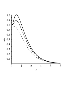
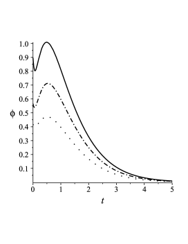
Figure 1: Plots of $\varphi(t)$ for different values of the constants $C_{1,2}^{u}$ . On the left , $C_{1}^{u}=2$ and $C^{u}_{2}$ takes the following values: $C_{2}^{u}=5$ (solid line), $C_{2}^{u}=4$ (dashed line) and $C_{2}^{u}=3$ (dotted line). On the right , $C_{2}^{u}=5$ and $C^{u}_{1}$ takes the following values: $C_{1}^{u}=2$ (solid line), $C_{1}^{u}=3$ (dash-dotted line) and $C_{1}^{u}=4$ (space-dotted line). Note that the solid lines on the left and right sides are the same curve.

Now we are ready to investigate numerically the $m=0$ solutions, obtained from substituting (5.18) and (5.2.1), together with (5.15) and (B.2), into (5.1). On Figure 1 we have plotted the scalar $\varphi(t)$ for different choices of $C_{1,2}^{u}$. On the left $C_{1}^{u}=const$, while $C_{2}^{u}$ varies. In this case, the initial value of $\varphi$ at $t=0$ stays the same, although the shape of the function $\varphi(t)$ changes. In particular, increasing $C_{2}^{u}$ increases $\varphi$. On the right of Figure 1, $C_{2}^{u}=const$ and $C_{1}^{u}$ varies. Clearly, now the initial value of $\varphi$ also changes. However, increasing $C_{1}^{u}$ decreases $\varphi$. In all of the cases on Figure 1, $\varphi$ starts at a finite value at $t=0$ and $\varphi\rightarrow 0$ as $t\rightarrow\infty$. Note that $\varphi=0$ is precisely the minimum of the potential (B.1).

On Figure 2 we have plotted the trajectories $\big{(}\varphi(t),\theta(t)\big{)}$ obtained for the same values of the constants $C_{1,2}^{u}$ as in Figure 1. At $t=0$ these trajectories start at $\theta=\frac{\pi}{2}$, while as $t\rightarrow\infty$ they tend to $\varphi=0$. In fact, it is more illuminating to plot them in polar coordinates. For easier comparison with the punctured disk and annuli cases, on Figure 3 we plot these trajectories in terms of the canonical radial variable of the Poincaré disk $\rho\in[0,1)$ , which is related to $\varphi$ via (2.5) .

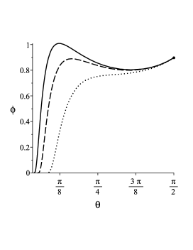
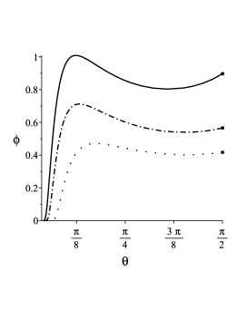
Figure 2: The trajectories $\big{(}\varphi(t),\theta(t)\big{)}$ for the same values of the constants as in Figure 1. The dot at one end of a trajectory denotes its starting point at $t=0$.

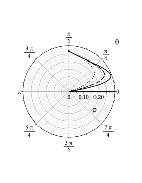
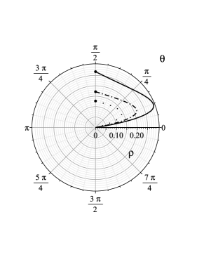
Figure 3: The trajectories $\big{(}\rho(t),\theta(t)\big{)}$, with $\rho$ being the radial variable on the unit disk, for the same values of the constants as in Figure 1.

Clearly, when $C_{1}^{u}=const$ and $C_{2}^{u}$ varies, the starting point at $t=0$ remains the same, although the shape of the trajectory changes. When $C_{2}^{u}=const$ and $C_{1}^{u}$ varies, the starting point changes as well. In both cases, though, the trajectories start at $t=0$ at a finite $\rho$ and as $t\rightarrow\infty$ they tend to $\rho=0$ , or equivalently $\varphi=0$ , which is the minimum of the potential (B.1).

Finally, on Figure 4 we plot the Hubble parameters $H(t)=\frac{\dot{a}(t)}{a(t)}$ for the same trajectories studied above. In all cases, we have $H(t)\rightarrow 1$ as $t\rightarrow\infty$. So the spacetimes, corresponding to these solutions, asymptote to dS space. Note that the horizontal axis starts at $t=0.4$ only for better visibility of the distinctions between the graphs. In each case, $H(0)$ is finite. For example, $H(0)=3.2$ for the solid line that is common for the left and right sides.

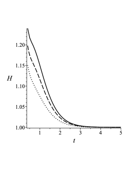
Figure 4: The Hubble parameters $H(t)$ for the same values of the constants as in Figure 1.

B.2 Hyperbolic punctured disk

The $m=0$ potential for the hyperbolic punctured disk case is:

$$V(\varphi,\theta)=V_{0}\,\exp\!\left(-\sqrt{\frac{3}{2}}\,\varphi\right)\,,$$ (B.4)

as one can see from (8). To obtain the single-field limit, we also need $w=const\times u$ (implying that $\theta=const$), as discussed in Section 6. However, by appropriately choosing the integration constants in (6.12) and (6.2), we can have $w\neq const\times u$ although $m=0$. So, in this case too, there are nontrivial two-field trajectories, even when the scalar potential does not depend on $\theta$. Before turning to their numerical investigation, it will be useful to write down explicitly the inverse of (2.8). Substituting $\alpha=\frac{4}{3}$, according to (3.3), gives:

$$\rho=\exp\!\left(-e^{\frac{\sqrt{6}}{4}\,\varphi}\right)\,,$$ (B.5)

where we have also used that by definition $\rho<1$ (see Appendix A).

We will explore, again, the dependence of the $(\varphi,\theta)$ trajectories on the two integration constants characterizing $u(t)$, namely $C_{1}^{*}$ and $C_{2}^{*}$, while keeping all the other constants fixed. In the process, a certain complementarity between the two constants in $u(t)$ will become even more apparent. It is convenient to take:

$$C_{w}=1\,\,,\,\,V_{0}=3\,\,,\,\,\Sigma_{*}=2\,\,,\,\,C_{0}^{w}=0\,\,,\,\,C_{4}^{*}=1\,\,,$$ (B.6)

while solving the constraint (6.18) for $C_{3}^{*}$. To ensure, with the choices (B.6), that the scale factor $a(t)>0$ for every $t\geq 0$ and that (6.18) can be solved, we need:

$$C_{2}^{*}>0\qquad{\rm and}\qquad C_{1}^{*}C_{3}^{*}>2\,\,.$$ (B.7)

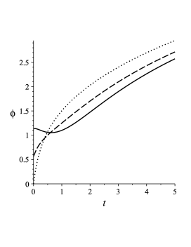
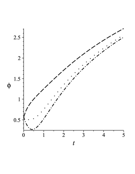
Figure 5: Plots of $\varphi(t)$ for different values of $C_{1,2}^{*}$ . On the left , $C_{1}^{*}=1$ and $C^{*}_{2}$ takes the values: $C_{2}^{*}=\frac{1}{2}$ (solid line), $C_{2}^{*}=1$ (dashed line) and $C_{2}^{*}=2$ (dotted line). On the right , $C_{2}^{*}=1$ and $C^{*}_{1}$ takes the values: $C_{1}^{*}=1$ (dashed line), $C_{1}^{*}=2$ (space-dotted line) and $C_{1}^{*}=3$ (dash-dotted line). Note that the dashed lines on the left and right sides are the same curve.

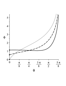
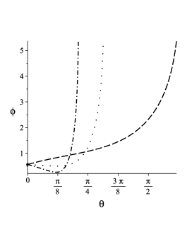
Figure 6: The trajectories $\big{(}\varphi(t),\theta(t)\big{)}$ for the same values of the constants as in Figure 5. The dot at one end of a trajectory denotes its starting point at $t=0$.

Let us now turn to the numerical investigation of the solutions, obtained by substituting (6.12) and (6.2), together with (6.9) and (B.6), into (6.1). On Figure 5 we plot $\varphi(t)$; on the left $C_{1}^{*}=const$ and $C_{2}^{*}$ varies, while on the right $C_{2}^{*}=const$ and $C_{1}^{*}$ varies. In all cases $\varphi\rightarrow\infty$ as $t\rightarrow\infty$. This is in perfect agreement with the fact that the minimum of the potential (B.4) is achieved for $\varphi\rightarrow\infty$. Note that, due to (B.5), $\varphi\rightarrow\infty$ corresponds to $\rho\rightarrow 0$.

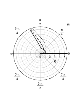
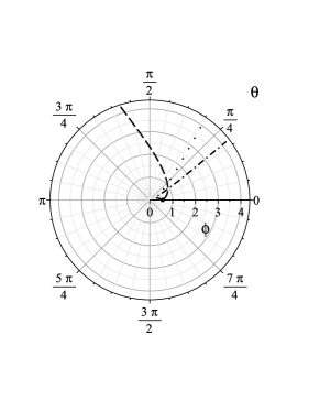
Figure 7: The trajectories of Figure 6 in polar $(\varphi,\theta)$ coordinates.

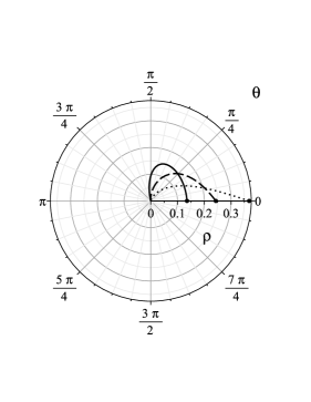
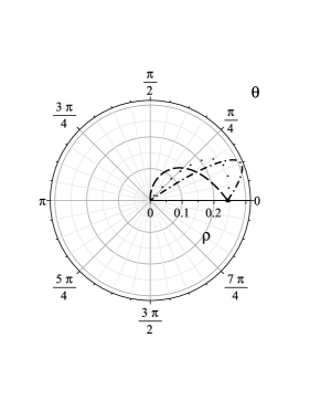
Figure 8: The trajectories $\big{(}\rho(t),\theta(t)\big{)}$ for the same values of the constants as in Figure 5.

On Figure 6 we plot the trajectories $\big{(}\varphi(t),\theta(t)\big{)}$ for the same values of the constants as in Figure 5. On the left, for different choices of $C_{2}^{*}$ (with $C_{1}^{*}$ fixed) the trajectories start at $t=0$ at different values of $\varphi$, while they all tend to $\varphi\rightarrow\infty$ and $\theta=\frac{5\pi}{8}$ as $t\rightarrow\infty$. On the right, for different values of $C_{1}^{*}$ (with $C_{2}^{*}$ fixed) all trajectories start at the same point, while for $t\rightarrow\infty$ they tend to different values of $\theta$. This is even more clear in polar $(\varphi,\theta)$ coordinates; see Figure 7. For easier comparison with the disk and annuli cases, on Figure 8 we also plot the same trajectories in polar $(\rho,\theta)$ coordinates, with $\rho\in(0,1)$ being the canonical radial variable of the hyperbolic punctured disk. Note that at $t=0$, the different trajectories start at different $\rho$, but as $t\rightarrow\infty$ they all tend to $\rho=0$, which corresponds to the minimum of the scalar potential.

Finally, on Figure 9 we plot the Hubble parameters corresponding to the trajectories considered above. In all cases, $H(t)|_{t=0}$ is finite and $H(t)\rightarrow 0$ as $t\rightarrow\infty$. This is in accordance with the fact that, for large $t$, the scalar $\varphi\rightarrow\infty$ and thus the potential (B.4), i.e. the effective cosmological constant, tends to zero. So the spacetimes of these solutions tend to Minkowski space. This may represent a natural mechanism for relaxation of the cosmological constant. Or it may indicate that this class of models has to be considered only in a finite time-range, assuming that at later times a different effective description (for example, containing new fields) would become more appropriate.

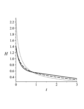
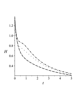
Figure 9: The Hubble parameters $H(t)$ for the same values of the constants as in Figure 5.

B.3 Hyperbolic Annuli

For the hyperbolic annuli case, the $m=0$ potential is:

$$V(\varphi,\theta)=V_{0}\,\sinh^{2}\!\left(\sqrt{\frac{3}{8}}\,\varphi\right)\,\,,$$ (B.8)

according to (8). From Section 7, it is clear that the single-field limit is obtained when, in addition, one has $w=const\times v$, which implies $\theta=const$. However, just like in Appendices B.1 and B.2, one can have $w\neq const\times v$ even when $m=0$, for suitable choices of the integration constants in (7.10) and (7.2.1). So, again, one can have nontrivial $(\varphi,\theta)$ trajectories, even though the potential is independent of $\theta$. To study numerically those trajectories, it will be convenient to use the canonical radial variable $\rho$ of the hyperbolic annuli, which is related to $\varphi$ via (2.11). Note that the inverse transformation (with $\alpha=\frac{4}{3}$ substituted) is:

$$\ln\rho=\frac{2}{C_{R}}\arctan\!\left[\tanh\!\left(\frac{\sqrt{6}}{8}\,\varphi\right)\right]\,,$$ (B.9)

where $\varphi\in(-\infty,\infty)$, with $\varphi<0$ corresponding to $\rho<1$ and $\varphi>0$ corresponding to $\rho>1$.

As before, we will study numerically the dependence of the nontrivial two-field trajectories on the integration constants in $u(t)$, i.e. on $C_{1}^{u}$ and $C_{2}^{u}$, with all other constants fixed. For convenience, let us take the following values:

$$C_{4}=0\,\,,\,\,C_{5}=\frac{1}{\sqrt{3}}\,\,,\,\,C_{w}=30\,\,,\,\,V_{0}=3\,\,,\,\,\Sigma_{0}=2\,\,,\,\,C_{0}^{w}=1\,\,,\,\,C_{2}^{v}=3\,\,,\,\,\hat{R}=2\,\,,$$ (B.10)

with $C_{1}^{v}$ determined from the Hamiltonian constraint (7.16). This, in particular, means that we are considering the annulus given by:

$$\frac{1}{2}<\rho<2\,\,.$$ (B.11)

Note that, with the choices (B.10), we need to have:

$$(C_{2}^{u})^{2}<23\,\,,$$ (B.12)

in order to ensure that $a(t)>0$ for any $t\geq 0$ . Finally, unlike in Appendices B.1 and B.2, the Hamiltonian constraint in this case does not impose any restriction on the choices of $C_{1}^{u}$ and $C_{2}^{u}$.

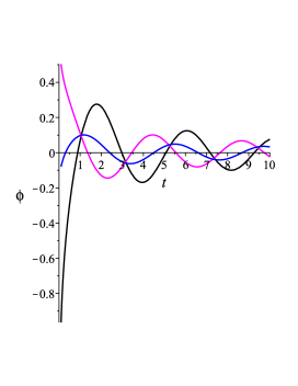
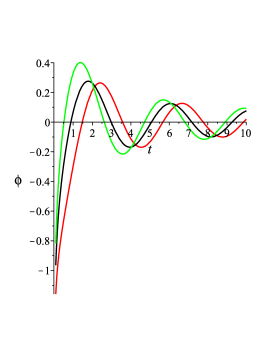
Figure 10: Plots of $\varphi(t)$ for several values of $C_{1,2}^{u}$ . On the left , $C_{1}^{u}=1$ and $C^{u}_{2}$ takes the values: $C_{2}^{u}=-4$ (black line), $C_{2}^{u}=-\frac{1}{2}$ (blue line) and $C_{2}^{u}=2$ (magenta line). On the right , $C_{2}^{u}=-4$ and $C^{u}_{1}$ takes the values: $C_{1}^{u}=-3$ (red line), $C_{1}^{u}=1$ (black line) and $C_{1}^{u}=4$ (green line). Note that the black lines on the left and right sides are the same curve.

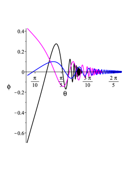
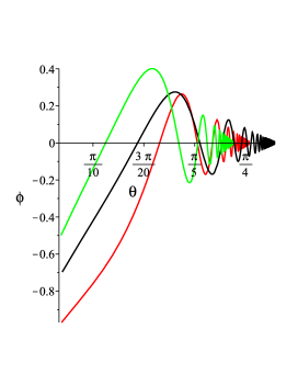
Figure 11: The trajectories $\big{(}\varphi(t),\theta(t)\big{)}$ for the same values of the constants as in Figure 10.

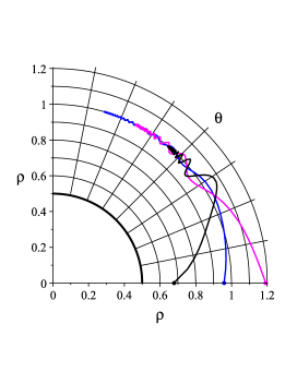
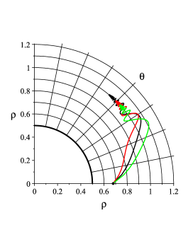
Figure 12: The trajectories $\big{(}\rho(t),\theta(t)\big{)}$ for the same values of the constants as in Figure 10. The dot at one end of a trajectory denotes its starting point at $t=0$.

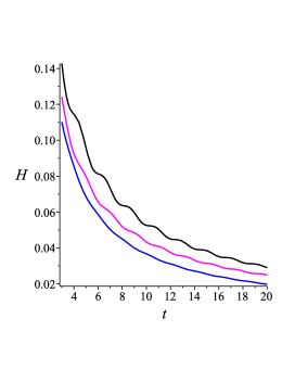
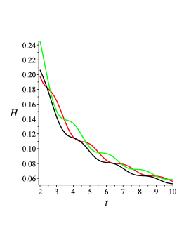
Figure 13: The Hubble parameters $H(t)$ for the same values of the constants as in Figure 10.

Now we turn to studying numerically the $m=0$ solutions, obtained from substituting (7.10) and (7.2.1), together with (B.10), into (7.1). On Figure 10 we plot $\varphi(t)$; on the left $C_{1}^{u}=const$ and $C_{2}^{u}$ changes, while on the right $C_{2}^{u}=const$ and $C_{1}^{u}$ changes. Note that in all cases $\varphi(0)$ is finite; this is not obvious, because we have started the plots at $t=0.1$ in order to make the overall features of the graphs better visible. Also, on the right side $\varphi(0)=-1.67$ for all three graphs. Notice that in all cases $\varphi(t)$ oscillates around $\varphi=0$ with an ever decreasing amplitude. Eventually, as $t\rightarrow\infty$, the scalar $\varphi(t)$ settles at $\varphi=0$, which is the minimum of the potential (B.8). This is even more clear on Figure 11, where we plot the trajectories $\big{(}\varphi(t),\theta(t)\big{)}$ for the same values of the constants as in Figure 10. The plots on Figure 11 start at $t=0.2$ , again for better visibility of the features of the graphs at large $t$. (They end at $t=140$.) This obscures the fact that all trajectories on the right side start at the same point. To illustrate clearly the entirety of the trajectories, it is most useful to change variables from $\varphi$ to the radial coordinate $\rho\in(\frac{1}{2},2)$ of the hyperbolic annulus. On Figure 12 we plot the trajectories $\big{(}\rho(t),\theta(t)\big{)}$ for the same values of the constants as in Figure 10. We have restricted the plot to the segment with $\theta\in[0,\frac{\pi}{2}]$ , in order to make the graphs better visible. Clearly, they all oscillate around $\rho=1$ with decreasing amplitudes and, as $t\rightarrow\infty$, they settle at $\rho=1$ and different values of $\theta$. Note that, due to (B.9), $\rho=1$ corresponds precisely to $\varphi=0$, which is the minimum of the scalar potential (B.8). It is also interesting to observe that trajectories, which start closer to $\rho=1$, reach greater values of $\theta$ as $t\rightarrow\infty$, although trajectories starting further from $\rho=1$ have greater amplitudes early on.

Finally, on Figure 13 we plot the Hubble parameters for the same trajectories as in Figures 10 - 12. We have restricted the range of $t$ from below only to make the distinctions between the graphs, as well as their features, visible. For each curve, $H(0)$ is finite and $H(t)\rightarrow 0$ as $t\rightarrow\infty$. This is in agreement with the fact that at late times $\varphi$ settles at $\varphi=0$ and so the potential (B.8) vanishes. This conclusion is similar to the one at the end of Appendix B.2. However, the present case has the rather peculiar feature that $H(t)$ exhibits a damped oscillations pattern. Thus, this class of models describes a kind of a cascading spacetime evolution. It would be interesting to explore whether, considered in a finite-time range, a transient stage of this kind (at the time of horizon exit of the largest observable CMB scales) might be helpful for explaining low multipole-moment anomalies in the CMB.

References

- [1] R. Kallosh, A. Linde and D. Roest, Superconformal Inflationary -Attractors, JHEP 11 (2013) 098, arXiv:1311.0472 [hep-th].
- [2] R. Kallosh, A. Linde and D. Roest, Large field inflation and double -attractors, JHEP 08 (2014) 052, arXiv:1405.3646 [hep-th].
- [3] R. Kallosh and A. Linde, Universality Class in Conformal Inflation, JCAP 1307 (2013) 002, arXiv:1306.5220 [hep-th].
- [4] R. Kallosh and A. Linde, Multi-field Conformal Cosmological Attractors, JCAP 1312 (2013) 006, arXiv:1309.2015 [hep-th].
- [5] R. Kallosh and A. Linde, Escher in the Sky, Comptes Rendus Physique 16 (2015) 914-927, arXiv:1503.06785 [hep-th].
- [6] J. Carrasco, R. Kallosh, A. Linde and D. Roest, The Hyperbolic Geometry of Cosmological Attractors, Phys. Rev. D 92 (2015) 041301, arXiv:1504.05557 [hep-th].
- [7] A. Achucarro, R. Kallosh, A. Linde, D. Wang and Y. Welling, Universality of multi-field -attractors, JCAP 04 (2018) 028, arXiv:1711.09478 [hep-th].
- [8] A. Linde, D. Wang, Y. Welling, Y. Yamadaa and A. Achucarro, Hypernatural inflation, JCAP 07 (2018) 035, arXiv:1803.09911 [hep-th].
- [9] M. Dias, J. Frazer, A. Retolaza, M. Scalisi and A. Westphal, Pole N-flation, arXiv:1805.02659 [hep-th].
- [10] A. R. Brown, Hyperbolic Inflation, Phys. Rev. Lett. 121, no. 25, 251601 (2018), arXiv:1705.03023 [hep-th].
- [11] S. Mizuno and S. Mukohyama, Primordial perturbations from inflation with a hyperbolic field-space, Phys. Rev. D 96, no. 10, 103533 (2017), arXiv:1707.05125 [hep-th].
- [12] P. Christodoulidis, D. Roest and E. I. Sfakianakis, Angular inflation in multi-field -attractors, arXiv:1803.09841 [hep-th].
- [13] S. Garcia-Saenz, S. Renaux-Petel and J. Ronayne, Primordial fluctuations and non-Gaussianities in sidetracked inflation, JCAP 1807, no.07, 057 (2018) arXiv:1804.11279 [astro-ph.CO].
- [14] C. I. Lazaroiu and C. S. Shahbazi, Generalized two-field -attractor models from geometrically finite hyperbolic surfaces, Nucl. Phys. B 936 (2018) 542-596, arXiv:1702.06484 [hep-th].
- [15] E. M. Babalic and C. I. Lazaroiu, Generalized -attractor models from elementary hyperbolic surfaces, Adv. Math. Phys. 2018 (2018) 7323090, arXiv:1703.01650 [hep-th].
- [16] E. M. Babalic and C. I. Lazaroiu, Generalized -attractors from the hyperbolic triply-punctured sphere, Nucl. Phys. B 937 (2018) 434, arXiv:1703.06033 [hep-th].
- [17] E. M. Babalic and C. I. Lazaroiu, Two-field cosmological models and the uniformization theorem, Springer Proc. Math. Stat. 255 (2017) 233, arXiv:1801.03356[hep-th].
- [18] G. Obied, H. Ooguri, L. Spodyneiko and C. Vafa, De Sitter Space and the Swampland, arxiv:1806.08362 [hep-th].
- [19] S. Garg and C. Krishnan, Bounds on Slow Roll and the de Sitter Swampland, arXiv:1807.05193 [hep-th].
- [20] W. H. Kinney, S. Vagnozzi and L. Visinelli, The Zoo Plot Meets the Swampland: Mutual (In)Consistency of Single-Field Inflation, String Conjectures, and Cosmological Data, arXiv:1808.06424 [astro-ph.CO].
- [21] A. Achucarro and G. Palma, The string swampland constraints require multi-field inflation, arXiv:1807.04390 [hep-th].
- [22] F. Denef, A. Hebecker and T. Wrase, The dS swampland conjecture and the Higgs potential, arXiv:1807.06581 [hep-th].
- [23] M. Cicoli, S. de Alwis, A. Maharana, F. Muia and F. Quevedo, De Sitter vs Quintessence in String Theory, arXiv:1808.08967 [hep-th].
- [24] S. Kachru and S. Trivedi, A comment on effective field theories of flux vacua, arXiv:1808.08971 [hep-th].
- [25] Y. Akrami, R. Kallosh, Andrei Linde and V. Vardanyan, The landscape, the swampland and the era of precision cosmology, arXiv:1808.09440 [hep-th].
- [26] H. Murayama, M. Yamazaki and T. Yanagida, Do We Live in the Swampland?, arXiv:1809.00478 [hep-th].
- [27] S. Capozziello and R. de Ritis, Relation between the potential and nonminimal coupling in inflationary cosmology, Phys. Lett. A177 (1993), 1.
- [28] S. Capozziello, G. Marmo, C. Rubano and P. Scudellaro, Noether symmetries in Bianchi universes, Int. J. Mod. Phys. D6 (1997) 491, gr-qc/9606050.
- [29] S. Capozziello, S. Nesseris and L. Perivolaropoulos, Reconstruction of the Scalar-Tensor Lagrangian from a LCDM Background and Noether Symmetry, JCAP 0712, 009 (2007), arXiv:0705.3586 [astro-ph].
- [30] S. Capozziello and A. De Felice, Cosmology by Noether’s symmetry, JCAP 0808:016,2008, arXiv:0804.2163 [gr-qc].
- [31] N. Kaewkhao, T. Kanesom and P. Channuie, Noether Symmetry Approach in the Cosmological Alpha-attractors, Nucl. Phys. B931 (2018) 216-225, arXiv:1711.10080 [gr-qc].
- [32] N. Bartolo, D. Bianco, R. Jimenez, S. Matarrese and L. Verde, Supergravity, -attractors and primordial non-Gaussianity, arXiv:1805.04269 [astro-ph.CO].
- [33] Y. Akrami, R. Kallosh, A. Linde and V. Vardanyan, Dark energy, -attractors, and large-scale structure surveys, JCAP 1806 (2018) 041, arXiv:1712.09693 [hep-th].
- [34] J. Ellis, B. Nagaraj, D. Nanopoulos and K. Olive, De Sitter Vacua in No-Scale Supergravity, arXiv:1809.10114 [hep-th].
- [35] E. Cremmer, J. Scherk and S. Ferrara, Invariant Supergravity Theory, Phys. Lett. B 74, 61 (1978).
- [36] E. M. Babalic, C. I. Lazaroiu, Cosmological flows on hyperbolic surfaces, arXiv:1810.00441 [hep-th].