The oblique firehose instability in a bi-kappa magnetized plasma

Abstract

In this work, we derive a dispersion equation that describes the excitation of the oblique (or Alfvén) firehose instability in a plasma that contains both electron and ion species modelled by bi-kappa velocity distribution functions. The equation is obtained with the assumptions of low-frequency waves and moderate to large values of the parallel (respective to the ambient magnetic field) plasma beta parameter, but it is valid for any direction of propagation and for any value of the particle gyroradius (or Larmor radius). Considering values for the physical parameters typical to those found in the solar wind, some solutions of the dispersion equation, corresponding to the unstable mode, are presented. In order to implement the dispersion solver, several new mathematical properties of the special functions occurring in a kappa plasma are derived and included. The results presented here suggest that the superthermal characteristic of the distribution functions leads to reductions to both the maximum growth rate of the instability and of the spectral range of its occurrence.

I Introduction

The plasma environment found in the interplanetary space is, in its majority, formed by particles of solar origin transported by the solar wind. The solar wind plasma is composed by electrons, protons, alpha particles and some other minority ions. Although the measured velocity distribution functions (VDFs) for each of the major populations have some specific characteristics, they also feature some common traits, such as high-energy isotropic or nonisotropic tails and high-energy beam populations that are aligned with the local interplanetary magnetic field (IMF).(Marsch, 2006)

One of the most important characteristics shown by the ion VDFs is a marked and conspicuous anisotropy in the velocity spreads measured in the direction parallel to the IMF with the spread measured in the perpendicular direction. These anisotropic velocity spreads are called in the literature temperature anisotropies and are measured by the second moments of the VDF, respectively evaluated in the parallel (the parallel temperature) and perpendicular (the perpendicular temperature) directions.

The importance of the presence of a temperature anistropy for the dynamical evolution of the solar wind plasma is that its departure from a themodynamic equilibrium state means that the plasma contains free energy sources in the particle distributions that can be tapped to excite several different plasma instabilities which will be ultimately responsible for several phenomena observed in the solar wind such as wave emission, particle energization and turbulence.(Klein and Howes, 2015)

In spite of the fact that other observed nonequilibrium features such as particle beams also offer free energy sources, a large part of the work published in the literature is concerned with the temperature anisotropy-driven instabilities (TADI). If we restrict ourselves with the anisotropies caused by the proton VDFs, there are four instabilities that are usually studied: the electromagnetic ion-cyclotron (or proton cyclotron) instability (EMIC), roughly excited when $T_{\perp p}>T_{\parallel p}$, where $T_{\parallel(\perp)p}$ is the parallel (perpendicular) temperature of the proton VDF, the parallel proton firehose instability (PFH), excited when $T_{\parallel p}>T_{\perp p}$, the mirror instability (MI, when $T_{\perp p}>T_{\parallel p}$) and the oblique (or Alfvén) firehose instability (OFH, when $T_{\parallel p}>T_{\perp p}$).(Klein and Howes, 2015) These instabilities are grouped in such a way that the first two (EMIC and PFH) are usually studied in the direction parallel to the IMF, whereas the second couple (MI and OFH) occur in the oblique direction. Rather than giving a long list of publications on the subject, the Reader is referred to the recent review provided by Ref. Yoon, 2017, which also provides lengthier discussions both on the theoretical derivation of the instabilities from the kinetic theory of plasmas and about their importance for the physical processes that take place in the solar wind.

The vast majority of the theoretical work on the TADI has been done assuming that the VDFs of the solar wind species can be adequately fitted by a combination of Maxwellian and bi-Maxwellian distributions.(Klein and Howes, 2015; Yoon, 2017; Klein et al., 2018) However, a substantial fraction of observed VDFs display high-energy (superthermal) tails that are better fitted by some power-law dependence such as $f\left(\boldsymbol{v}\right)\propto v^{-2\kappa}$, where $f\left(\boldsymbol{v}\right)$ is the velocity distribution function and $0<\kappa<\infty$ is a fitting parameter.

The most frequently employed model of distribution with such power-law behavior is the kappa VDF,(Livadiotis, 2015) which describes the velocity distribution of a plasma species that is in a quasi-stationary state away from thermal equilibrium, where the particle interactions are long-ranged and where there are strong correlations among the degrees of freedom. With a $\kappa$VDF, the kappa parameter is a measure of the departure of the (quasi-)stationary state from thermal equilibrium: the smaller the value of $\kappa$ the farther from equilibrium, which is asymptotically reached when $\kappa\to\infty$. In practice, when $\kappa\gtrsim 20$ the $\kappa$VDF is already quasi-Maxwellian. A collection of works regarding the origin, observations, properties and the statistical mechanics of kappa distributions was recently organized by G. Livadiotis.(Livadiotis, 2017a)

It is already well established that the high energy populations of the electron VDF in the solar wind (the halo and the Strahl) are better modelled with kappa or bi-kappa distributions.(Maksimovic et al., 2005; Štverák et al., 2009; Pierrard et al., 2016) For both populations, it has been measured $\kappa_{e}<10$ for a wide range of heliocentric distances, ranging from 0.3 AU (Astronomical Units) to nearly 4 AU. In fact, the value of $\kappa_{e}$ reduces with distance, showing that the electrons in the solar wind are in a constant process of departure from thermal equilibrium as the solar wind propagates through the interplanetary space.

The observed distributions of the major ion species in the solar wind and some physical properties associated with the shape of the VDFs have also been analysed employing kappa distributions. Detailed discussions and a longer list of publications can be found in Refs. Pierrard and Pieters, 2014; Livadiotis, Desai, and Wilson, 2018. It has been verified that the ion VDFs are also well modelled with typical values of $\kappa_{i}\lesssim 5$.

Therefore, one must conclude that a full picture of the plasma instabilities operating in the solar wind can only be obtained if, in their theoretical description, the superthermal nature of the observed distributions are taken into account.

So far, of the four instabilities listed above, excited by temperature anisotropies in the ion VDFs, only those that occur in parallel-propagating modes (MTSI and PFH) have been systematicaly studied when $\kappa$ distributions are involved.(Lazar, Poedts, and Schlickeiser, 2011; Lazar, 2012; Lazar and Poedts, 2014; dos Santos, Ziebell, and Gaelzer, 2014, 2015, 2016a, 2016b; Ziebell and Gaelzer, 2017; Lazar et al., 2018) The Reader is referred to a recent review by Viñas et al.(Viñas et al., 2017) for a detailed theoretical account and further references.

By comparison, studies regarding instabilities that are excited by $\kappa$VDFs and that occur at oblique angles relative to the IMF are scant. One line of research has been focused on the development of computer codes that numerically evaluate the dielectric tensor of kappa distributions and solve the dispersion equation, thereby obtaining the dispersion relations of the several wavemodes and their associated damping/growth rates with an ab initio numerical procedure.(Sugiyama et al., 2015; Astfalk, Görler, and Jenko, 2015; Astfalk and Jenko, 2016)

Another line has emphasized the derivation of analytical and closed-form expressions for the dielectric tensor of a (bi-)kappa VDF. A first contribution considered the effect of the $\kappa$VDF on the propagation and damping of highly-oblique dispersive Alfvén waves in the Earth’s magnetosphere.(Gaelzer and Ziebell, 2014) Further contributions provided the closed-form expressions for the dielectric tensor of an isotropic kappa plasma in Ref. Gaelzer and Ziebell, 2016 and a bi-kappa plasma in Ref. Gaelzer, Ziebell, and Meneses, 2016. These publications will hereafter be addressed respectively as Papers I and II. Whenever possible, the derivation of analytical and closed-form expressions for the dielectric tensor is desirable, because they provide important information about the mathematical properties of the dispersion relations and allow the derivation of the dispersion equations for specific normal modes of propagation.

In this work, we will employ the formulation provided in Papers I and II in order to derive a dispersion equation suitable for the study of the oblique firehose instability excited by a bi-kappa plasma. The OFH, first discovered by Yoon et al.(Yoon, Wu, and de Assis, 1993) and later found again by Hellinger and Matsumoto,(Hellinger and Matsumoto, 2000) is an instability occurring in low-frequencies and at oblique angles, commonly associated with dispersive Alfvén waves.(Lysak and Lotko, 1996; Gaelzer and Ziebell, 2014) However, as we shall see below, the OFH is in fact an absolute instability associated with a nonpropagating mode. Here, we will derive a dispersion equation valid for plasmas with moderate values of the ion beta parameter and show some numerical results. In order to implement the dispersion relation solver, several new mathematical properties of the special functions ocurring in a kappa plasma were obtained, which were not presented in Papers I and II. Consequently, in this work we will present some typical solutions of the dispersion equation and reserve a more comprehensive and detailed analysis of the instability for a future publication.

The plan of the paper is as follows. In section II the specific dispersion equation is obtained. In section III, the new mathematical properties for the special functions are derived. Then, in section IV we present some solutions of the dispersion equation, which show the occurrence of the OFH. Finally, in section V we present our conclusions.

II Dispersion equation for a high-beta bi-kappa plasma

The general form of the dielectric tensor for a magnetized bi-kappa plasma can be found in Paper II, eqs. 2 and 3. For the present application, we will employ the kappa velocity distribution function ($\kappa$VDF) introduced first by Summers and Thorne,(Summers and Thorne, 1991) which can be obtained from the general form adopted in Papers I and II by setting the parameters $\alpha=1$ and $w_{\parallel(\perp)s}^{2}=\left(1-3/2\kappa_{s}\right)v_{T\parallel(\perp)s}^{2}$, where $s=e,i,\dots$ denotes the plasma species/population and $v_{T\parallel(\perp)s}^{2}=2T_{\parallel(\perp)s}/m_{s}$ is the thermal velocity squared of the same species. With this particular choice, the explicit expression of the $\kappa$VDF is obtained from (I.1) (i.e., equation 1 of Paper I) or from (II.1) and is given by

$$f_{s}\left(\boldsymbol{v}\right) =A_{s}^{(\kappa_{s})}\left(1+\frac{v_{\parallel}^{2}}{\kappa_{s}w_{\parallel s}^{2}}+\frac{v_{\perp}^{2}}{\kappa_{s}w_{\perp s}^{2}}\right)^{-\left(\kappa_{s}+1\right)}$$ (1)

$$A_{s}^{(\kappa_{s})} =\frac{1}{\pi^{3/2}w_{\parallel s}w_{\perp s}^{2}}\frac{\Gamma\left(\kappa_{s}+1\right)}{\kappa_{s}^{3/2}\Gamma\left(\kappa_{s}-\nicefrac{{1}}{{2}}\right)},\>\left(\kappa_{s}>\frac{1}{2}\right).$$

In accordance with the particular choices of the parameters $\alpha$ and $w_{\parallel(\perp)s}$ adopted here, the same settings must the imposed on the general expressions for the dielectric tensor and the kappa plasma functions discussed in Papers I and II.

The particular form of the $\kappa$VDF in (1) is the model more frequently employed in the literature for reasons that have been discussed at length in Ref. Gaelzer and Ziebell, 2014 and in Papers I and II.

Among the several new expressions introduced by Papers I and II regarding the physical properties of the propagation of electromagnetic/electrostatic waves and wave-particle interactions in a kappa plasma, for any combination of particle species and wave modes, frequency and polarization, a great amount of space was dedicated to the discussion of the mathematical properties and numerical evaluation of several special functions, namely, the kappa (or superthermal) plasma dispersion function $Z_{\kappa}^{\left(\alpha,\beta\right)}\left(\xi\right)$, the kappa plasma gyroradius function $\mathcal{H}_{n,\kappa}^{\left(\alpha,\beta\right)}\left(z\right)$ and the two-variables kappa plasma functions $\mathcal{Z}_{n,\kappa}^{\left(\alpha,\beta\right)}\left(\mu,\xi\right)$ and $\mathcal{Y}_{n,\kappa}^{\left(\alpha,\beta\right)}\left(\mu,\xi\right)$. The reader is referred to Papers I and II for the definitions of these functions and for the mentioned properties. Some new mathematical formulas and properties for the same functions, developed for the present application, are presented in section III below.

In order to reduce the amount of algebra, we will first define the quantity

$$1_{\kappa}^{\left(\beta\right)}=\frac{\Gamma\left(\kappa+\beta-1\right)}{\kappa^{\beta-1/2}\Gamma\left(\kappa-\nicefrac{{1}}{{2}}\right)},$$

which is such that $1_{\kappa}^{\left(\beta\right)}\xrightarrow{\kappa\to\infty}1$, and then define the following form for the kappa plasma gyroradius function,

$$\mathrm{H}_{n,\kappa}^{\left(\beta\right)}\left(\mu\right)=1_{\kappa}^{\left(\beta+1\right)}\mathcal{H}_{n,\kappa}^{\left(1,\beta\right)}\left(\mu\right).$$

We will also employ hereafter the shorthand notation $\mathcal{Z}_{n,\kappa}^{\left(\beta\right)}\left(\mu,\xi\right)$ and $\mathcal{Y}_{n,\kappa}^{\left(\beta\right)}\left(\mu,\xi\right)$, which implicitly assumes that we are taking the same functions with $\alpha=1$.

Given a plasma species $s$ composed by particles with mass $m_{s}$, electric charge $q_{s}$ and number density $n_{s}$, we start by taking the general form of the dielectric tensor in (II.2,3) and make the change $n\to-n$ for all the terms involving negative values of the harmonic index $n$, thereby obtaining

$$\varepsilon_{xx} =1+\sum_{s}\frac{\omega_{ps}^{2}}{\omega^{2}}\sum_{n=1}^{\infty}\frac{n^{2}}{\mu_{s}}\left(A_{ns,\kappa}+A_{-ns,\kappa}\right)$$ (2a)

$$\varepsilon_{xy} =i\sum_{s}\frac{\omega_{ps}^{2}}{\omega^{2}}\sum_{n=1}^{\infty}n\partial_{\mu_{s}}\left(A_{ns,\kappa}-A_{-ns,\kappa}\right)$$ (2b)

$$\varepsilon_{xz} =-\sum_{s}\frac{\omega_{ps}^{2}}{\omega^{2}}\frac{k_{\perp}w_{\parallel s}}{2\Omega_{s}}\sum_{n=1}^{\infty}\frac{n}{\mu_{s}}\left(B_{ns,\kappa}-B_{-ns,\kappa}\right)$$ (2c)

$$\varepsilon_{yy} =1+\sum_{s}\frac{\omega_{ps}^{2}}{\omega^{2}}\left[C_{0s,\kappa}+\sum_{n=1}^{\infty}\left(C_{ns,\kappa}+C_{-ns,\kappa}\right)\right]$$ (2d)

$$\varepsilon_{yz} =i\sum_{s}\frac{\omega_{ps}^{2}}{\omega^{2}}\frac{k_{\perp}w_{\parallel s}}{2\Omega_{s}}\left[\partial_{\mu_{s}}B_{0s,\kappa}\right.$$

$$\left.+\sum_{n=1}^{\infty}\partial_{\mu_{s}}\left(B_{ns,\kappa}+B_{-ns,\kappa}\right)\right]$$ (2e)

$$\varepsilon_{zz} =1-\sum_{s}\frac{\omega_{ps}^{2}}{\omega^{2}}\frac{v_{T\parallel s}^{2}}{v_{T\perp s}^{2}}\left[\xi_{0s}B_{0s,\kappa}\right.$$

$$\left.+\sum_{n=1}^{\infty}\left(\xi_{ns}B_{ns,\kappa}+\xi_{-ns}B_{-ns,\kappa}\right)\right],$$ (2f)

where $$\varepsilon_{ij} \left(i,j=x,y,z\right) \varepsilon_{xy}=-\varepsilon_{yx} \varepsilon_{xz}=\varepsilon_{zx} \varepsilon_{yz}=-\varepsilon_{zy} \partial_{\mu}=\partial/\partial\mu$$ are the components of the dielectric tensor, which obeys the usual symmetry relations , and . Also, ,

$$\mu_{s} =\frac{k_{\perp}^{2}w_{\perp s}^{2}}{2\Omega_{s}^{2}}=\left(1-\frac{3}{2\kappa_{s}}\right)\frac{k_{\perp}^{2}v_{T\perp s}^{2}}{2\Omega_{s}^{2}},$$

$$\xi_{ns} =\frac{\omega-n\Omega_{s}}{k_{\parallel}w_{\parallel s}}=\left(1-\frac{3}{2\kappa_{s}}\right)^{-\frac{1}{2}}\frac{\omega-n\Omega_{s}}{k_{\parallel}v_{T\parallel s}},$$

and $$\omega_{ps}^{2}=4\pi n_{s}q_{s}^{2}/m_{s} \Omega_{s}=q_{s}B_{0}/m_{s}c s \boldsymbol{B}_{0}=B_{0}\hat{\boldsymbol{z}} c \omega \boldsymbol{k}=k_{\perp}\hat{\boldsymbol{x}}+k_{\parallel}\hat{\boldsymbol{z}}$$ is the squared plasma and the cyclotron frequencies of species for a plasma embedded in an uniform ambient magnetic induction vector . Additionaly, is the light speed in vacuum and and are the usual (angular) frequency and wave vector of oscillations propagating in the plasma.

In (2a-f), the quantities $A$, $B$ and $C$ are defined as

$$A_{ns,\kappa} =\xi_{0s}\mathcal{Z}_{n,\kappa_{s}}^{\left(2\right)}\left(\mu_{s},\xi_{ns}\right)+\frac{1}{2}A_{s}\partial_{\xi_{ns}}\mathcal{Z}_{n,\kappa_{s}}^{\left(1\right)}\left(\mu_{s},\xi_{ns}\right)$$ (3a)

$$B_{ns,\kappa} =\left(\xi_{0s}-A_{s}\xi_{ns}\right)\partial_{\xi_{ns}}\mathcal{Z}_{n,\kappa_{s}}^{\left(1\right)}\left(\mu_{s},\xi_{ns}\right)$$ (3b)

$$C_{ns,\kappa} =\xi_{0s}\mathcal{W}_{n,\kappa_{s}}^{\left(2\right)}\left(\mu_{s},\xi_{ns}\right)+\frac{1}{2}A_{s}\partial_{\xi_{ns}}\mathcal{W}_{n,\kappa_{s}}^{\left(1\right)}\left(\mu_{s},\xi_{ns}\right),$$ (3c)

where

$$\mathcal{W}_{n,\kappa_{s}}^{\left(\beta\right)}\left(\mu_{s},\xi_{ns}\right)=\frac{n^{2}}{\mu_{s}}\mathcal{Z}_{n,\kappa_{s}}^{\left(\beta\right)}\left(\mu_{s},\xi_{ns}\right)-2\mu_{s}\mathcal{Y}_{n,\kappa_{s}}^{\left(\beta\right)}\left(\mu_{s},\xi_{ns}\right),$$

$$A_{s}=1-T_{\perp s}/T_{\parallel s} s \partial_{\xi}=\partial/\partial\xi$$ is the temperature anisotropy parameter for species , and .

In the present application, we are interested in low-frequency $(\omega\ll\left|\Omega_{s}\right|)$ and long-wavelength $\bigl{(}k_{\parallel}^{2}v_{T\parallel s}^{2}\ll\Omega_{s}^{2}\bigr{)}$ waves propagating in oblique directions relative to $\boldsymbol{B}_{0}$. In such a situation, $\omega_{ps}^{2}/\omega^{2}\gg\omega_{ps}^{2}/\Omega_{s}^{2}$, where

$$\frac{\omega_{ps}^{2}}{\Omega_{s}^{2}}=\frac{n_{s}m_{s}}{n_{i}m_{i}}\frac{c^{2}}{v_{A}^{2}},$$

with $s=i$ referring to the ion species and with the squared Alfvén speed $v_{A}^{2}=B_{0}^{2}/4\pi n_{i}m_{i}$. Hence, for an electron-ion plasma, if at least we have $\left(m_{e}/m_{i}\right)\left(c^{2}/v_{A}^{2}\right)\simeq 1$, then $\omega_{ps}^{2}/\omega^{2}\gg 1$ and we can neglect, as a first approximation, the displacement current terms (the unity) in the diagonal components of the dielectric tensor (2).

Now we notice that given the (squared) particle gyroradius (or Larmor radius) $\rho_{s}^{2}=v_{T\perp s}^{2}/2\Omega_{s}^{2}=T_{\perp s}/m_{s}\Omega_{s}^{2}$, the quantity $\mu_{s}$ can be written as $\mu_{s}=\left(1-3/2\kappa_{s}\right)k_{\perp}^{2}\rho_{s}^{2}$. Among the several low-frequency wave modes observed in the solar wind and Earth’s magnetosphere, of particular importance are the dispersive Alfvén waves (DAW).(Lysak and Lotko, 1996; Gaelzer and Ziebell, 2014) In regions where the plasma thermal effects on the wave dispersion can not be ignored, the DAW are known as the kinetic Alfvén waves (KAW). Measuring the thermal effect with the parallel/perpendicular plasma beta parameter $\beta_{\parallel(\perp)s}=8\pi n_{s}T_{\parallel(\perp)s}/B_{0}^{2}$, the dispersion relation of KAW propagating in an isotropic Maxwellian plasma with moderate values of the electron beta $\left(m_{e}/m_{i}\ll\beta_{e}\lesssim 1\right)$ is(Lysak and Lotko, 1996)

$$\frac{\omega^{2}}{k_{\parallel}^{2}v_{A}^{2}}\approx 1+k_{\perp}^{2}\left(\rho_{a}^{2}+\frac{3}{4}\rho_{i}^{2}\right),$$

where $\rho_{a}^{2}=T_{e}/m_{i}\Omega_{i}^{2}$ is the ion-acoustic gyroradius. Hence, for the ions, an estimate on the magnitude of the parameter $\mu_{i}$ for KAW is given by

$$\mu_{i}=\frac{1}{2}\left(1-\frac{3}{2\kappa_{i}}\right)\frac{k_{\perp}^{2}c^{2}}{\omega_{pi}^{2}}\beta_{\perp i}\approx\frac{1}{2}\left(1-\frac{3}{2\kappa_{i}}\right)\frac{\omega^{2}}{\Omega_{i}^{2}}\frac{k_{\perp}^{2}}{k_{\parallel}^{2}}\beta_{\perp i}.$$

Therefore, even for low-frequency Alfvén waves, the parameter $\mu_{i}$ can be small but finite when the ion beta is large and/or the KAW is propagating at large angles relative to $\boldsymbol{B}_{0}$.

Moreover, since we are assuming $\omega\ll\left|\Omega_{s}\right|$ and $k_{\parallel}^{2}v_{T\parallel s}^{2}\ll\Omega_{s}^{2}$, the typical $\left|\xi_{ns}\right|$ for $n\geqslant 1$ is supposed to be larger than the unity by several orders of magnitude. In this situation, we can employ in the coefficients $A_{ns,\kappa}$, $B_{ns,\kappa}$ and $C_{ns,\kappa}$ the asymptotic expansions given in (II.28a,b) for the functions $\mathcal{Z}_{n,\kappa}^{\left(\beta\right)}\left(\mu,\xi\right)$ and $\mathcal{Y}_{n,\kappa}^{\left(\beta\right)}\left(\mu,\xi\right)$, with their derivatives given by (II.22) and (11), keeping only the leading terms in the expansions. Then, defining the small parameters $x=\omega/n\Omega_{s}$ and $\epsilon=k_{\parallel}w_{\parallel s}/n\Omega_{s}$ for $n\geqslant 1$, expanding the combinations of the coefficients in (2) and (3) in powers of $x$ and $\epsilon$ and keeping only the lowest-order contributions, one obtains, after some algebra,

$$A_{ns,\kappa}+A_{-ns,\kappa} \approx\frac{2\omega^{2}}{n^{2}\Omega_{s}^{2}}\left[\vphantom{\frac{k_{\parallel}^{2}}{\omega^{2}}}\mathrm{H}_{n,\kappa_{s}}^{\left(\nicefrac{{3}}{{2}}\right)}\left(\mu_{s}\right)\right.$$

$$\left.+\frac{1}{2}A_{s}\mathrm{H}_{n,\kappa_{s}}^{\left(\nicefrac{{1}}{{2}}\right)}\left(\mu_{s}\right)\frac{k_{\parallel}^{2}w_{\parallel s}^{2}}{\omega^{2}}\right]$$

$$A_{ns,\kappa}-A_{-ns,\kappa} \approx\frac{2\omega}{n\Omega_{s}}\left[\vphantom{\frac{k_{\parallel}^{2}}{\omega^{2}}}\mathrm{H}_{n,\kappa_{s}}^{\left(\nicefrac{{3}}{{2}}\right)}\left(\mu_{s}\right)\right.$$

$$\left.+\frac{1}{2}\left(1+2A_{s}\right)\mathrm{H}_{n,\kappa_{s}}^{\left(\nicefrac{{1}}{{2}}\right)}\left(\mu_{s}\right)\frac{k_{\parallel}^{2}w_{\parallel s}^{2}}{n^{2}\Omega_{s}^{2}}\right]$$

$$B_{ns,\kappa}+B_{-ns,\kappa} \approx 2\left(A_{s}+1\right)\mathrm{H}_{n,\kappa_{s}}^{\left(\nicefrac{{1}}{{2}}\right)}\left(\mu_{s}\right)\frac{k_{\parallel}w_{\parallel s}}{n\Omega_{s}}\frac{\omega}{n\Omega_{s}}$$

$$B_{ns,\kappa}-B_{-ns,\kappa} \approx 2\mathrm{H}_{n,\kappa_{s}}^{\left(\nicefrac{{1}}{{2}}\right)}\left(\mu_{s}\right)A_{s}\frac{k_{\parallel}w_{\parallel s}}{n\Omega_{s}}$$

$$C_{ns,\kappa}+C_{-ns,\kappa} \approx 2\mathrm{G}_{n,\kappa_{s}}^{\left(\nicefrac{{3}}{{2}}\right)}\left(\mu_{s}\right)\frac{\omega^{2}}{n^{2}\Omega_{s}^{2}}$$

$$+A_{s}\mathrm{G}_{n,\kappa_{s}}^{\left(\nicefrac{{1}}{{2}}\right)}\left(\mu_{s}\right)\frac{k_{\parallel}^{2}w_{\parallel s}^{2}}{n^{2}\Omega_{s}^{2}}$$

$$\xi_{ns}B_{ns,\kappa}+\xi_{-ns}B_{-ns,\kappa}\approx-2\mathrm{H}_{n,\kappa}^{\left(\nicefrac{{1}}{{2}}\right)}\left(\mu_{s}\right)A_{s},$$

where

$$\mathrm{G}_{n,\kappa}^{\left(\beta\right)}\left(\mu\right)=\frac{n^{2}}{\mu}\mathrm{H}_{n,\kappa}^{\left(\beta\right)}\left(\mu\right)-2\mu\mathrm{H}_{n,\kappa}^{\left(\beta-1\right)\prime}\left(\mu\right).$$

Notice that the above approximations are only used for the terms with harmonic $n\neq 0$. In the expressions for $A_{0s,\kappa}$, $B_{0s,\kappa}$ and $C_{0s,\kappa}$, we have kept the full thermal effects for the kappa plasma functions.

Inserting these approximations back into (2), we observe that each component of the dielectric tensor contains a sum over $n\geqslant 1$ of the function $\mathrm{H}_{n,\kappa}^{\left(\beta\right)}\left(\mu\right)$ or its derivative. Making use of the identity (II.10), we can establish the sum rule

$$\sum_{n\to-\infty}^{\infty}\mathrm{H}_{n,\kappa}^{\left(\beta\right)}\left(\mu\right)=1_{\kappa}^{\left(\beta\right)},$$

whereby we can define the auxiliary functions

$$H_{1,\kappa}^{\left(\beta\right)}\left(\mu\right) =\frac{1_{\kappa}^{\left(\beta\right)}-\mathrm{H}_{0,\kappa}^{\left(\beta\right)}\left(\mu\right)}{\mu},$$ (4a)

$$H_{2,\kappa}^{\left(\beta\right)}\left(\mu\right) =2\sum_{n=1}^{\infty}\frac{\mathrm{H}_{n,\kappa}^{\left(\beta\right)\prime}\left(\mu\right)}{n^{2}},$$ (4b)

which were obtained by also making use of the property $$\mathrm{H}_{-n,\kappa}^{\left(\beta\right)}\left(\mu\right)=\mathrm{H}_{n,\kappa}^{\left(\beta\right)}\left(\mu\right) H_{1,\kappa}^{\left(\beta\right)}\left(0\right)=H_{2,\kappa}^{\left(\beta\right)}\left(0\right)=1_{\kappa}^{(\beta-1)}$$. Additionaly, by virtue of (I.21) and the identity found at the top of page 4 of Paper II, we have .

Apropos, the Maxwellian limits of functions $H_{1,\kappa}^{\left(\beta\right)}$ and $H_{2,\kappa}^{\left(\beta\right)}$ are

$$H_{1}\left(\mu\right) =\frac{1-\mathscr{H}_{0}\left(\mu\right)}{\mu}=1-\frac{3}{4}\mu+\frac{5}{12}\mu^{2}+\cdots$$

$$H_{2}\left(\mu\right) =2\sum_{n=1}^{\infty}\frac{\mathscr{H}_{n}^{\prime}\left(\mu\right)}{n^{2}}=1-\frac{15}{8}\mu+\frac{245}{144}\mu^{2}+\cdots,$$

where $\mathscr{H}_{n}\left(\mu\right)=e^{-\mu}I_{n}\left(\mu\right)$. The small gyroradius expansion of $H_{1}\left(\mu\right)$ presented above is well known and easily obtained from the properties of the modified Bessel function. However, the function $H_{2}\left(\mu\right)$ has always been presented in closed form and, to the best of the authors’ knowledge, no series expansion was known in the literature (see, e.g., Refs. Yoon, Wu, and de Assis, 1993; Lysak and Lotko, 1996). The derivation of the series expansion for $H_{2}\left(\mu\right)$ will be given in a future publication.

Finaly, considering a 2-species electron-ion plasma, we define the following parameters, which are inspired by and generalize the corresponding parameters given in Ref. Yoon, Wu, and de Assis, 1993,

$$\epsilon_{\kappa}^{\left(\beta\right)} =H_{1,\kappa_{i}}^{\left(\beta\right)}\left(\mu_{i}\right)$$ (5a)

$$\epsilon_{\kappa}^{\left(\beta\right)\prime} =\epsilon_{\kappa}^{\left(\beta\right)}-2\mu_{i}H_{2,\kappa_{i}}^{\left(\beta-1\right)}\left(\mu_{i}\right)$$ (5b)

$$\hat{\epsilon}_{\kappa} =-\left[\frac{Z_{\kappa_{e}}^{\left(0\right)\prime}\left(\xi_{0e}\right)}{\beta_{\parallel e,\kappa}}+\frac{1}{\beta_{\parallel i,\kappa}}\partial_{\xi_{0i}}\mathcal{Z}_{0,\kappa_{i}}^{\left(1\right)}\left(\mu_{i},\xi_{0i}\right)\right]\frac{\beta_{\perp i,\kappa}}{2\mu_{i}}$$ (5c)

$$\gamma_{\kappa} =\frac{1}{2}\left(\beta_{\parallel e}A_{e}+\beta_{\parallel i,\kappa}A_{i}\epsilon_{\kappa}^{\left(\nicefrac{{1}}{{2}}\right)}-2\right)\frac{k_{\parallel}^{2}v_{A}^{2}}{\Omega_{i}^{2}}$$ (5d)

$$\gamma_{\kappa}^{\prime} =\frac{1}{2}\left(\beta_{\parallel e}A_{e}+\beta_{\parallel i,\kappa}A_{i}\epsilon_{\kappa}^{\left(\nicefrac{{1}}{{2}}\right)\prime}-2\right)\frac{k_{\parallel}^{2}v_{A}^{2}}{\Omega_{i}^{2}}$$

$$-\left[1+\beta_{\perp e,\kappa}\left(1_{\kappa_{e}}^{\left(-\nicefrac{{1}}{{2}}\right)}+\frac{1}{2}\frac{\beta_{\perp e,\kappa}}{\beta_{\parallel e,\kappa}}Z_{\kappa_{e}}^{\left(-2\right)\prime}\left(\xi_{0e}\right)\right)\right.$$

$$-\beta_{\perp i,\kappa}\left(\vphantom{\frac{\beta_{\perp i,\kappa}}{\beta_{\parallel i,\kappa}}}\mathrm{H}_{0,\kappa_{i}}^{\left(\nicefrac{{1}}{{2}}\right)\prime}\left(\mu_{i}\right)\right.$$

$$\left.\left.+\frac{1}{2}\frac{\beta_{\perp i,\kappa}}{\beta_{\parallel i,\kappa}}\partial_{\xi_{0i}}\mathcal{Y}_{0,\kappa_{i}}^{\left(1\right)}\left(\mu_{i},\xi_{0i}\right)\right)\right]\frac{2\mu_{i}}{\beta_{\perp i,\kappa}}$$ (5e)

$$\eta_{\kappa} =1_{\kappa_{e}}^{\left(\nicefrac{{1}}{{2}}\right)}+\mathrm{H}_{0,\kappa_{i}}^{\left(\nicefrac{{3}}{{2}}\right)\prime}\left(\mu_{i}\right)$$

$$-\frac{1}{2}\left(1+2A_{i}\right)\beta_{\parallel i,\kappa}H_{2,\kappa_{i}}^{\left(\nicefrac{{1}}{{2}}\right)}\left(\mu_{i}\right)\frac{k_{\parallel}^{2}v_{A}^{2}}{\Omega_{i}^{2}}$$ (5f)

$$\eta_{\kappa}^{\prime} =-\frac{\beta_{\perp e,\kappa}}{2\beta_{\parallel e,\kappa}}Z_{\kappa_{e}}^{\left(-1\right)\prime}\left(\xi_{0e}\right)-\frac{\beta_{\perp i,\kappa}}{2\beta_{\parallel i,\kappa}}\partial_{\mu_{i}}\partial_{\xi_{0i}}\mathcal{Z}_{0,\kappa_{i}}^{\left(1\right)}\left(\mu_{i},\xi_{0i}\right)$$

$$-\frac{1}{2}\beta_{\parallel i,\kappa}\left(1+A_{i}\right)H_{2,\kappa_{i}}^{\left(\nicefrac{{1}}{{2}}\right)}\left(\mu_{i}\right)\frac{k_{\parallel}^{2}v_{A}^{2}}{\Omega_{i}^{2}},$$ (5g)

where we have also defined the kappa-modified beta parameters as

$$\beta_{\parallel(\perp)s,\kappa}=\left(1-\frac{3}{2\kappa_{s}}\right)\beta_{\parallel(\perp)s}=\frac{\beta_{\parallel(\perp)s}}{1_{\kappa_{s}}^{(-\nicefrac{{1}}{{2}})}}.$$

We must also point out that since $$\mu_{e}\ll\mu_{i} m_{e}/m_{i} H_{1,\kappa_{e}}^{\left(\beta\right)}\left(\mu_{e}\right)\approx H_{2,\kappa_{e}}^{\left(\beta\right)}\left(\mu_{e}\right)\approx 1_{\kappa_{e}}^{(\beta-1)}$$ by a factor of order , we have kept in parameters (5a-g) the lowest-order gyroradius contribution from the electrons, i.e., .

The parameters (5a-g) are identified within the dispersion equation $\det\mathsf{\Lambda}=0$, where the elements of the matrix $\mathsf{\Lambda}$ are

$$\Lambda_{ij}=\frac{c^{2}}{\omega^{2}}\left(k_{i}k_{j}-k^{2}\delta_{ij}\right)+\boldsymbol{\varepsilon}_{ij},\;\left(i,j=x,y,z\right).$$

After some algebraic manipulation, during the course of which some other terms that are of order $m_{e}/m_{i}$ are neglected, one notices that one root $\omega^{2}\approx 0$ can be factored out and the remaining equation can be written in transcendental form as

$$\left(\frac{\omega}{\Omega_{i}}\right)^{4}+\left[\frac{1}{\epsilon_{\kappa}^{\left(\nicefrac{{3}}{{2}}\right)\prime}}\left(\gamma_{\kappa}^{\prime}-\frac{\eta_{\kappa}^{2}}{\epsilon_{\kappa}^{\left(\nicefrac{{3}}{{2}}\right)}}-\frac{\eta_{\kappa}^{\prime 2}}{\hat{\epsilon}_{\kappa}}\right)\right.\\ \left.+\gamma_{\kappa}\left(\frac{1}{\epsilon_{\kappa}^{\left(\nicefrac{{3}}{{2}}\right)}}+\frac{1}{\hat{\epsilon}_{\kappa}}\right)\right]\left(\frac{\omega}{\Omega_{i}}\right)^{2}+\frac{\gamma_{\kappa}}{\epsilon_{\kappa}^{\left(\nicefrac{{3}}{{2}}\right)\prime}}\\ \times\left[\gamma_{\kappa}^{\prime}\left(\frac{1}{\epsilon_{\kappa}^{\left(\nicefrac{{3}}{{2}}\right)}}+\frac{1}{\hat{\epsilon}_{\kappa}}\right)-\frac{\left(\eta_{\kappa}-\eta_{\kappa}^{\prime}\right)^{2}}{\epsilon_{\kappa}^{\left(\nicefrac{{3}}{{2}}\right)}\hat{\epsilon}_{\kappa}}\right]=0.$$ (6)

Some of the particular cases of equation (6) are discussed below.

II.1 Maxwellian limit

If one takes the limits $\kappa_{e}\to\infty$ and $\kappa_{i}\to\infty$, one observes that $1_{\kappa}^{(\beta)}\xrightarrow{\kappa\to\infty}1$, and the limits of the kappa plasma functions are given in Papers I and II. In this case, the dispersion equation (6), as well as the parameters (5a-g) reduce to the corresponding forms given by Ref. Yoon, Wu, and de Assis, 1993, as expected.

II.2 Limit of parallel propagation

In the limit $k_{\perp}\to 0$ or, equivalently, the limit of zero ion gyroradius, we have $\mu_{i}\to 0$, and we have to employ the limiting forms given by (I.21), (II. 23), the expression given in page 04 of Paper II, and (12). As a result, the dispersion equation (6) reduces to

$$\left(\frac{\omega^{2}}{\Omega_{i}^{2}}+\eta\frac{\omega}{\Omega_{i}}+\gamma\right)\left(\frac{\omega^{2}}{\Omega_{i}^{2}}-\eta\frac{\omega}{\Omega_{i}}+\gamma\right)=0,$$

$$\begin{aligned} \gamma&=\frac{1}{2}\left(\beta_{\parallel e}A_{e}+\beta_{\parallel i}A_{i}-2\right)\frac{k_{\parallel}^{2}v_{A}^{2}}{\Omega_{i}^{2}}\\ \eta&=-\frac{1}{2}\left(1+2A_{i}\right)\beta_{\parallel i}\frac{k_{\parallel}^{2}v_{A}^{2}}{\Omega_{i}^{2}},\end{aligned}$$

which is exactly the same solution obtained by Ref. Yoon, Wu, and de Assis, 1993.

In this case, the dispersion relations are the roots of polynomials that only depend on the wavenumber, the plasma betas and the anisotropy parameters. In other words, the dispersion equation (6) predicts that the kappa parameters $\kappa_{e}$ and $\kappa_{i}$ do not influence the parallel firehose instability.

An exact treatment of the PFH shows a different picture. Whereas the real part of the dispersion relation is largely independent on the kappas, the growth rate does depend on $\kappa_{e}$ and, mostly, on $\kappa_{i}$. The reason why the treatment presented here is not able to account for this fact lies with the assumptions made about the magnitudes of the quantities $\left|\xi_{\pm e}\right|$ and $\left|\xi_{\pm i}\right|$. When $k_{\perp}=0$, the ion-firehose occurs in the right-handed mode (the magnetosonic mode). A careful examination of the unstable range shows that the nonresonant approximations $\left|\xi_{\pm e}\right|\gg 1$ and $\left|\xi_{+i}\right|\gg 1$ are still valid, but $\left|\xi_{-i}\right|\simeq 1$. Hence, for the parallel firehose instability the kinetic effects due to this quantity can not be ignored and the growth rate is no longer given by the simple root of a polynomial, as above. A detailed account of the PFH in a bi-kappa plasma is given by Ref. Viñas et al., 2017.

II.3 Limit of perpendicular propagation

In the converse case $\left(k_{\parallel}\to 0\right)$, one must consider in (5a-g) the asymptotic forms of the kappa plasma functions for the limits $\xi_{0e},\xi_{0i}\to\infty$. For the function $Z_{\kappa}^{\left(\beta\right)}\left(\xi\right)$ one can notice in the expansion given by the expression at page 14 of Paper I that the dominant term is $Z_{\kappa}^{\left(\beta\right)}\left(\xi\right)\simeq-1_{\kappa}^{\left(\beta+\nicefrac{{1}}{{2}}\right)}/\xi$. For the functions $\mathcal{Z}$ and $\mathcal{Y}$, one employs again the dominant terms of expansions (II.28a,b).

After some manipulations, equation (6) factors into two branches: $\omega^{2}=0$ and

$$\left(\frac{\omega}{\Omega_{i}}\right)^{2} =\frac{1}{\epsilon_{\kappa}^{\left(\nicefrac{{3}}{{2}}\right)\prime}}\left(d_{3\kappa}+\frac{d_{4\kappa}^{2}}{\epsilon_{\kappa}^{\left(\nicefrac{{3}}{{2}}\right)}}\right),\text{ where}$$

$$d_{3\kappa} =\left[1+\beta_{\perp e}-\beta_{\perp i,\kappa}\mathrm{H}_{0,\kappa_{i}}^{\left(\nicefrac{{1}}{{2}}\right)\prime}\left(\mu_{i}\right)\right]\frac{2\mu_{i}}{\beta_{\perp i,\kappa}}$$

$$d_{4\kappa} =1_{\kappa_{e}}^{\left(\nicefrac{{1}}{{2}}\right)}+\mathrm{H}_{0,\kappa_{i}}^{\left(\nicefrac{{3}}{{2}}\right)\prime}\left(\mu_{i}\right).$$

In the Maxwellian limit, the expression of the nonzero mode, in the lowest-order of a small gyroradius expansion, is

$$\omega\simeq\sqrt{1+\beta_{\perp e}+\beta_{\perp i}}k_{\perp}v_{A},$$

which corresponds to the dispersion relation of compressive Alfvén waves. These waves are always damped. On the other hand, the nonpropagating mode with $\omega^{2}=0$ turns out to be the unstable mode.

For any combination of $\left(k_{\perp},k_{\parallel}\right)$, the wave modes are obtained from the numerical solution of equation (6). Several new properties of the kappa plasma functions, not included in Papers I and II, were needed in order to implement the numerical solution of the dispersion equation. These properties are discussed in section III, and some numerical solutions are presented in section IV.

III New expressions for the kappa plasma special functions

Several new properties and representations for the kappa special functions are developed here.

III.1 Symmetry properties of the superthermal plasma dispersion function

The superthermal (or kappa) plasma dispersion function ($\kappa$PDF) $Z_{\kappa}^{\left(\alpha,\beta\right)}\left(\xi\right)$ was initially defined in (I.11) and several properties were presented in Papers I and II. Here, we will show its symmetry properties, which will be important for the new expansions of the functions $\mathcal{Z}$ and $\mathcal{Y}$ to be presented below.

Consider first the argument $\xi=\xi_{r}+i\xi_{i}\in\mathbb{C}$. If $\xi_{i}>0$, one of the possible representations of $Z_{\kappa}^{\left(\alpha,\beta\right)}\left(\xi\right)$ is given by (I.13), while its analytic continuation for $\xi_{i}\leqslant 0$ is given by (I.A1). Hence, we can directly establish the first identity, when $\xi_{i}>0$,

$$Z_{\kappa}^{\left(\alpha,\beta\right)}\left(-\xi\right)+Z_{\kappa}^{\left(\alpha,\beta\right)}\left(\xi\right)\\ =2i\sqrt{\pi}\frac{\kappa^{-\beta-1/2}\Gamma\left(\lambda-1\right)}{\Gamma\left(\sigma-\nicefrac{{3}}{{2}}\right)}\left(1+\frac{\xi^{2}}{\kappa}\right)^{-\left(\lambda-1\right)}.$$ (7a)

As discussed in Papers I and II, when $\alpha=\beta=1$, the function $Z_{\kappa}^{\left(1,1\right)}\left(\xi\right)\equiv Z_{\kappa}\left(\xi\right)$ reduces to the dispersion function first introduced by Summers and Thorne(Summers and Thorne, 1991) and largely discussed by Mace and Hellberg(Mace and Hellberg, 1995). In this case, the symmetry property above reduces to Eq. 27 of Ref. Mace and Hellberg, 1995. In the Maxwellian limit $\left(\kappa\to\infty\right)$, the same property reduces to the known identity for the Fried & Conte function,(Fried and Conte, 1961)

$$Z\left(-\xi\right)+Z\left(\xi\right)=2i\sqrt{\pi}e^{-\xi^{2}},\>\left(\xi_{i}>0\right).$$

Now, let us consider the representation (I.14), which is valid in the principal branch $-\frac{1}{2}\pi<\arg\left(\xi+i\sqrt{\kappa}\right)<\frac{3}{2}\pi$ (i.e., the branch line runs along $-i\sqrt{\kappa}<\xi<-i\infty$). This is the generalization of the result given by Eq. 17 of Ref. Mace and Hellberg, 1995. If we denote by $\bar{\xi}=\xi_{r}-i\xi_{i}$ the operation of complex conjugation, we immediately observe that

$$Z_{\kappa}^{\left(\alpha,\beta\right)}\left(-\bar{\xi}\right) =i\frac{\kappa^{-\beta-1/2}\Gamma\left(\lambda-\nicefrac{{1}}{{2}}\right)}{\left(\lambda-1\right)\Gamma\left(\sigma-\nicefrac{{3}}{{2}}\right)}$$

$$\times\prescript{\vphantom{2}}{2}{F}_{1}^{\vphantom{1}}\left[{1,2\left(\lambda-1\right)\atop\lambda};\frac{1}{2}\left(1-\frac{i\bar{\xi}}{\kappa^{1/2}}\right)\right].$$

However, given that

$$\prescript{\vphantom{2}}{2}{F}_{1}^{\vphantom{1}}\left({\bar{a},\bar{b}\atop\bar{c}};\bar{z}\right)=\overline{\prescript{\vphantom{2}}{2}{F}_{1}^{\vphantom{1}}\left({a,b\atop c};z\right)}\quad\left(z\notin\left(1,\infty\right)\right),$$

which is a property shared by all hypergeometric functions in their principal branches, it follows that

$$Z_{\kappa}^{\left(\alpha,\beta\right)}\left(\bar{\xi}\right)=-\overline{Z_{\kappa}^{\left(\alpha,\beta\right)}\left(-\xi\right)}.$$ (7b)

This result also reduces to the known property $Z\left(\bar{\xi}\right)=-\overline{Z\left(-\xi\right)}$.

Finally, by combining properties (7a) and (7b), we obtain, for $\xi_{i}>0$,

$$Z_{\kappa}^{\left(\alpha,\beta\right)}\left(\bar{\xi}\right) =\overline{Z_{\kappa}^{\left(\alpha,\beta\right)}\left(\xi\right)}$$ (7c)

$$+2i\sqrt{\pi}\frac{\kappa^{-\beta-1/2}\Gamma\left(\lambda-1\right)}{\Gamma\left(\sigma-\nicefrac{{3}}{{2}}\right)}\left(1+\frac{\bar{\xi}^{2}}{\kappa}\right)^{-\left(\lambda-1\right)},$$

which, when $\kappa\to\infty$, reduces to

$$Z\left(\bar{\xi}\right)=\overline{Z\left(\xi\right)}+2i\sqrt{\pi}e^{-\bar{\xi}^{2}}.$$

III.2 The superthermal plasma gyroradius function

The kappa plasma gyroradius function ($\kappa$PGF) $\mathcal{H}_{n,\kappa}^{\left(\alpha,\beta\right)}\left(z\right)$ was initially defined by (I.20) and its more general representation was given by (I.22) in terms of the Meijer $G$-function. The definition and properties of the $G$-function can be seen in appendix B of Paper I or in the references given therein. Several properties of $\mathcal{H}_{n,\kappa}^{\left(\alpha,\beta\right)}\left(z\right)$ and an associated function are discussed in Papers I and II. Here we will present some new properties of the $\kappa$PGF.

III.2.1 Symmetry properties

In some of the representations shown in Papers I and II as well as in the present work, the function $\mathcal{H}_{n,\kappa}^{\left(\alpha,\beta\right)}\left(z\right)$ needs to be evaluated for complex $z$. Looking at the representations (I.23, 24), respectively valid for noninteger/integer values of $\lambda=\kappa+\alpha+\beta$, and taking into account the symmetry properties of elementary and Bessel functions, one readily concludes (i) that the $\kappa$PGF is a multivalued function with the origin as a branch point and with a branch cut along the negative real axis, and (ii) that in the principal branch,

$$\mathcal{H}_{n,\kappa}^{\left(\alpha,\beta\right)}\left(\bar{z}\right)=\overline{\mathcal{H}_{n,\kappa}^{\left(\alpha,\beta\right)}\left(z\right)},\qquad\left(\left|\arg z\right|<\pi\right).$$ (8)

III.2.2 Series expansion in the integer case

As it was argued at length in Papers I and II, the function $\mathcal{H}_{n,\kappa}^{\left(\alpha,\beta\right)}\left(z\right)$ can be represented in terms of power series only when $\lambda=\kappa+\alpha+\beta$ is not integer. When $\lambda\in\mathbb{Z}$, the function has a logarithmic term and a representation in terms of modified Bessel functions was given by (I.24) (see Eq. II.7c for the derivatives). Although general, the evaluation of $\mathcal{H}_{n,\kappa}^{\left(\alpha,\beta\right)}\left(z\right)$ via the Bessel functions can be computationally expensive when $\left|z\right|<1$, as is the case for the application discussed in this paper. Hence, a suitable series expansion for $\mathcal{H}_{n,\kappa}^{\left(\alpha,\beta\right)}\left(z\right)$ in the regime of small gyroradius is desired.

The desired representation is obtained via the residue theorem. Using (I.22) and (I.B10), the function $\mathcal{H}_{n,\kappa}^{\left(\alpha,\beta\right)}\left(z\right)$ can be written as

$$\mathcal{H}_{n,\kappa}^{\left(\alpha,\beta\right)}\left(z\right) =\frac{1}{\sqrt{\pi}}\frac{\kappa}{\Gamma\left(\lambda-1\right)}F_{n,\lambda-2}\left(2\kappa z\right),$$ (9a)

$$F_{n,\theta}\left(z\right) =\frac{1}{2\pi i}\int_{L}f_{n,\theta}\left(s\right)z^{-s}ds,$$

$$f_{n,\theta}\left(s\right) =\frac{\Gamma\left(\theta+s\right)\Gamma\left(n+s\right)\Gamma\left(\nicefrac{{1}}{{2}}-s\right)}{\Gamma\left(n+1-s\right)},$$

where the integration contour $$L \Gamma\left(\theta+s\right) \Gamma\left(n+s\right) L \Gamma\left(\nicefrac{{1}}{{2}}-s\right)$$ is such that all poles of and lie to the right of whereas the poles of lie to the left. In this case, the residues of the integration are given only by the poles of the first two gamma functions.

If $m\in\mathbb{Z}$, when $\theta=m$ (for $\mathcal{H}_{n,\kappa}^{\left(\alpha,\beta\right)}$, $m=0,1,2,\dots$), the poles of $f_{n,\theta}\left(s\right)$ occur at $s=-m-r$ and $s=-n-r$ $\left(r\in\mathbb{N}\right)$. Hence, there are two possibilities: (i) $m<n$ and (ii) $m\geqslant n$, that will be treated separately.

1. $\boldsymbol{m<n}$:

the function $f_{n,\theta}\left(s\right)$ has simple poles at $s=-m,-m-1,\dots,-n+1$ and double poles at $s=-n,-n-1,\dots$. The residues of the simple poles can be evaluated with the identity

$$\Gamma\left(z\right)=\frac{\left(-\right)^{k}}{k!\left(z+k\right)}+\frac{\left(-\right)^{k}}{k!}\psi\left(k+1\right)+\mathcal{O}\left[\left(z+k\right)\right],$$

where $\psi\left(z\right)$ is the psi or digamma function. This expansion is valid for $z\simeq-k$ $\left(k=0,1,2,\dots\right)$. Therefore,

$$\mathrm{Res}f_{n,\theta}\left(s=-\ell\right)=\sqrt{\pi}\left(-\right)^{m}\frac{\Gamma\left(n-\ell\right)\left(\nicefrac{{1}}{{2}}\right)_{\ell}}{\left(1\right)_{n+\ell}\left(1\right)_{\ell-m}}\left(-z\right)^{\ell},$$

where $\ell=m,m+1,\dots,n-1$ and $\left(a\right)_{r}=\Gamma\left(a+r\right)/\Gamma\left(a\right)$ is the Pochhammer symbol.

On the other hand, the double poles are obtained from

$$\mathrm{Res}f_{n,\theta}\left(s=-\ell\right)=\lim_{s\to-\ell}\frac{d}{ds}\left[\left(s+\ell\right)^{2}f_{n,\theta}\left(s\right)\right],$$

for $\ell=n,n+1,\dots$. Given that $\Gamma^{\prime}\left(z\right)=\psi\left(z\right)\Gamma\left(z\right)$, and using the identity

$$\psi\left(z\right)=-\frac{1}{z+k}+\psi\left(k+1\right)+\mathcal{O}\left[\left(z+k\right)\right],$$

one obtains for the residues

$$\mathrm{Res}f_{n,\theta}\left(s=-\ell\right) =\frac{\sqrt{\pi}\left(\nicefrac{{1}}{{2}}\right)_{\ell}\left(-\right)^{m+n}z^{\ell}}{\left(1\right)_{n+\ell}\left(1\right)_{\ell-m}\left(1\right)_{\ell-n}}$$

$$\times\left[\vphantom{\frac{1}{2}}\psi\left(\ell-m+1\right)+\psi\left(\ell-n+1\right)\right.$$

$$\left.-\psi\left(\frac{1}{2}+\ell\right)+\psi\left(n+\ell+1\right)-\ln z\right].$$

2. $\boldsymbol{m\geqslant n}$:

now the poles are simple for $s=-n,\dots,-m+1$ $\left(m>n\right)$ and double for $s=-m,-m-1,\dots$. The evaluation of the residues follows the same lines as in the previous case.

Summing the contributions from all residues, both possibilities can be cast in a single expression for $F_{n,\theta}\left(z\right)$, resulting finally

$$\frac{F_{n,\theta}\left(z\right)}{\sqrt{\pi}} =\epsilon_{\sigma}\left(\sigma-1\right)!\left(\frac{1}{2}\right)_{\nu}\frac{z^{\nu}}{\eta!}\sum_{\ell=0}^{\sigma-1}\frac{\left(\nu+\nicefrac{{1}}{{2}}\right)_{\ell}}{\left(\eta+1\right)_{\ell}\left(1-\sigma\right)_{\ell}}\frac{z^{\ell}}{\ell!}$$ (9b)

$$-\left(-\right)^{\nu}\left(\frac{1}{2}\right)_{\mu}\frac{\left(-z\right)^{\mu}}{\psi!\sigma!}$$

$$\times\left[\left(2\gamma+\ln z\right)\prescript{\vphantom{1}}{1}{F}_{2}^{\vphantom{2}}\left({\mu+\nicefrac{{1}}{{2}}\atop\psi+1,\sigma+1};z\right)\right.$$

$$-\sum_{\ell=0}^{\infty}\frac{\left(\mu+\nicefrac{{1}}{{2}}\right)_{\ell}}{\left(\psi+1\right)_{\ell}\left(\sigma+1\right)_{\ell}}$$

$$\left.\times\left(H_{\ell}+H_{\psi+\ell}+H_{\sigma+\ell}-H_{\mu-\nicefrac{{1}}{{2}}+\ell}\right)\frac{z^{\ell}}{\ell!}\right],$$

where $\mu=\max\left(\theta,n\right)$, $\nu=\min\left(\theta,n\right)$, $\sigma=\mu-\nu$, $\psi=\mu+n$, $\eta=\nu+n$, and $\epsilon_{\sigma}=1-\delta_{\sigma,0}$. In (9b), the quantities $H_{w}$ are the harmonic numbers, given by $H_{w}=\psi\left(w+1\right)+\gamma$, where $\gamma=0.57721\dots$ is Euler’s constant. When $w$ is a nonnegative integer, the harmonic numbers are $H_{0}=0$ and $H_{\ell}=\sum_{k=1}^{\ell}k^{-1}$.

Notice that there are two terms in (9b) that distinguishes the series expansion of $\mathcal{H}_{n,\kappa}^{\left(\alpha,\beta\right)}\left(z\right)$ when $\lambda$ is integer from a simple power series expansion of the hypergeometric kind. First, there is a term proportional to $\ln z$ and second, the last term is a power series but is not hypergeometric.

III.3 The two-variables kappa plasma functions

The two-varibles kappa plasma functions (2VKPs) $\mathcal{Z}_{n,\kappa}^{\left(\alpha,\beta\right)}\left(\mu,\xi\right)$ and $\mathcal{Y}_{n,\kappa}^{\left(\alpha,\beta\right)}\left(\mu,\xi\right)$ were initially defined by (I.26). They describe the dispersive properties of oscillations occuring in a magnetized (bi-)kappa plasma. Since a magnetized plasma described by a $\kappa$VDF displays strong correlations between the parallel and perpendicular components of the particles’ velocities, the 2VKPs can not be factored as the product of two simple functions; i.e., there are no functions $M\left(\mu\right)$ and $N\left(\xi\right)$ such that $\mathcal{Z}\left(\mu,\xi\right)=M\left(\mu\right)N\left(\xi\right)$, for instance. This point has been argued at length in Ref. Gaelzer and Ziebell, 2014 and in Papers I and II. Consequently, the simpler representations one can expect for these functions will always be some transcendental series expansion.

III.3.1 Symmetry properties

The symmetry properties of the functions $\mathcal{Z}_{n,\kappa}^{\left(\alpha,\beta\right)}\left(\mu,\xi\right)$ and $\mathcal{Y}_{n,\kappa}^{\left(\alpha,\beta\right)}\left(\mu,\xi\right)$ can be readily derived starting from the integral representations (I.26a,b). For applications to plasma physics, $\mu>0$ always but $\xi$ is in general complex. Hence, the symmetry properties of the 2VKPs are determined by the $Z_{\kappa}^{\left(\alpha,\beta\right)}\left(\xi\right)$ function.

Consequently, from the symmetry properties (7), one concludes that

$$\mathcal{Z}_{n,\kappa}^{\left(\alpha,\beta\right)}\left(\mu,\bar{\xi}\right) =-\overline{\mathcal{Z}_{n,\kappa}^{\left(\alpha,\beta\right)}\left(\mu,-\xi\right)}$$ (10a)

$$\mathcal{Y}_{n,\kappa}^{\left(\alpha,\beta\right)}\left(\mu,\bar{\xi}\right) =-\overline{\mathcal{Y}_{n,\kappa}^{\left(\alpha,\beta\right)}\left(\mu,-\xi\right)}$$ (10b)

$$\mathcal{Z}_{n,\kappa}^{\left(\alpha,\beta\right)}\left(\mu,\bar{\xi}\right) =\overline{\mathcal{Z}_{n,\kappa}^{\left(\alpha,\beta\right)}\left(\mu,\xi\right)}$$

$$+2i\sqrt{\pi}\frac{\kappa^{-1/2-\beta}\Gamma\left(\lambda-1\right)}{\Gamma\left(\sigma-\nicefrac{{3}}{{2}}\right)}\left(1+\frac{\bar{\xi}^{2}}{\kappa}\right)^{-\left(\lambda-2\right)}$$

$$\times\mathcal{H}_{n,\kappa}^{\left(\alpha,\beta\right)}\left[\mu\left(1+\frac{\bar{\xi}^{2}}{\kappa}\right)\right]$$ (10c)

$$\mathcal{Y}_{n,\kappa}^{\left(\alpha,\beta\right)}\left(\mu,\bar{\xi}\right) =\overline{\mathcal{Y}_{n,\kappa}^{\left(\alpha,\beta\right)}\left(\mu,\xi\right)}$$

$$+2i\sqrt{\pi}\frac{\kappa^{1/2-\beta}\Gamma\left(\lambda-2\right)}{\Gamma\left(\sigma-\nicefrac{{3}}{{2}}\right)}\left(1+\frac{\bar{\xi}^{2}}{\kappa}\right)^{-\left(\lambda-4\right)}$$

$$\times\mathcal{H}_{n,\kappa}^{\left(\alpha,\beta-1\right)\prime}\left[\mu\left(1+\frac{\bar{\xi}^{2}}{\kappa}\right)\right].$$ (10d)

For the derivation of (10c) and (10d) we have employed the identities (II.24, 26).

Moreover, it can be easily verified that

$$\mathcal{Z}_{-n,\kappa}^{\left(\alpha,\beta\right)}\left(\mu,\xi\right) =\mathcal{Z}_{n,\kappa}^{\left(\alpha,\beta\right)}\left(\mu,\xi\right),$$ (10e)

$$\mathcal{Y}_{-n,\kappa}^{\left(\alpha,\beta\right)}\left(\mu,\xi\right) =\mathcal{Y}_{n,\kappa}^{\left(\alpha,\beta\right)}\left(\mu,\xi\right).$$

Henceforth, we will implicitly assume that $n\geqslant 0$.

III.3.2 Derivative of $\boldsymbol{\mathcal{Y}_{n,\kappa}^{\left(\alpha,\beta\right)}\left(\mu,\xi\right)}$

As can be observed in the expressions for the dielectric tensor given either by (II.3) or by (2) and (3), one also needs to evaluate $\partial_{\xi}\mathcal{Y}_{n,\kappa}^{\left(\alpha,\beta\right)}\left(\mu,\xi\right)$. The expressions for this derivative were not included in Paper II due to an oversight, which will be remedied now.

The procedure is roughly the same as the one described in section C.1 of Paper II for the function $\mathcal{Z}$. So, without further ado, we present

$$\partial_{\xi}\mathcal{Y}_{n,\kappa}^{\left(\alpha,\beta\right)}\left(\mu,\xi\right) =-2\left[\frac{\Gamma\left(\lambda-\nicefrac{{3}}{{2}}\right)}{\kappa^{\beta}\Gamma\left(\sigma-\nicefrac{{3}}{{2}}\right)}\mathcal{H}_{n,\kappa}^{\left(\alpha,\beta-\nicefrac{{1}}{{2}}\right)\prime}\left(\mu\right)\right.$$

$$\left.+\xi\mathcal{Y}_{n,\kappa}^{\left(\alpha,\beta+1\right)}\left(\mu,\xi\right)\vphantom{\frac{\Gamma\left(\lambda-\nicefrac{{3}}{{2}}\right)}{\Gamma\left(\sigma-\nicefrac{{3}}{{2}}\right)}}\right],$$ (11)

with the particular case,

$$\partial_{\xi}\mathcal{Y}_{n,\kappa}^{\left(\alpha,\beta\right)}\left(0,\xi\right)=\left(-\delta_{n,0}+\frac{1}{2}\delta_{\left|n\right|,1}\right)Z_{\kappa}^{\left(\alpha,\beta-3\right)\prime}\left(\xi\right).$$ (12)

III.3.3 Power series expansions for large $\boldsymbol{\left|\xi\right|}$

Power series expansions for $\mathcal{Z}$ and $\mathcal{Y}$ were given by (II.25a) and (II.27a), which are formally convergent for $\left|\xi\right|<\sqrt{\kappa}$. Additionally, other series expansions were given by (II.25c) and (II.27b), which are formally valid for the whole complex plane of $\xi$. However, for the range of variations of the physical parameters considered in this work, although the argument $\mu$ is always small, since it is proportional to the particle’s gyroradius, the magnitude of the argument $\xi=\xi_{0s}=\omega/k_{\parallel}w_{\parallel s}$ can vary from very small (for near-parallel propagation) to very large (for near-perpendicular propagation). Hence, from the computational point of view it is desirable to have power series expansions for the 2VKPs valid for $\left|\xi\right|>\sqrt{\kappa}$. These series will now be derived.

We will consider first the function $\mathcal{Z}_{n,\kappa}^{\left(\alpha,\beta\right)}\left(\mu,\xi\right)$. Taking the integral representation (I.26a) and inserting representation (II.15a) for $Z_{\kappa}^{\left(\alpha,\beta\right)}\left(\xi\right)$, we can integrate the last term using identity (II.24) and obtain

$$\mathcal{Z}_{n,\kappa}^{\left(\alpha,\beta\right)}\left(\mu,\xi\right) =-2\frac{\pi^{1/2}\kappa^{-\beta-1/2}}{\Gamma\left(\sigma-\nicefrac{{3}}{{2}}\right)}\frac{\xi}{\sqrt{\kappa}}F_{2}\left(\mu,\xi\right)+\frac{i\pi^{1/2}\Gamma\left(\lambda-1\right)}{\kappa^{\beta+1/2}\Gamma\left(\sigma-\nicefrac{{3}}{{2}}\right)}\left(1+\frac{\xi^{2}}{\kappa}\right)^{-\left(\lambda-2\right)}\mathcal{H}_{n,\kappa}^{\left(\alpha,\beta\right)}\left[\mu\left(1+\frac{\xi^{2}}{\kappa}\right)\right],$$

$$F_{2}\left(\mu,\xi\right) =\int_{0}^{\infty}dx\,\frac{xJ_{n}^{2}\left(\sqrt{2\mu}\,x\right)}{\left(1+x^{2}/\kappa\right)^{\lambda-1/2}}G_{2,2}^{1,2}\left[\frac{\xi^{2}/\kappa}{1+x^{2}/\kappa}\left|{0,\nicefrac{{3}}{{2}}-\lambda\atop 0,-\nicefrac{{1}}{{2}}}\right.\right],$$

where $G_{2,2}^{1,2}$ is the Meijer $G$-function defined by (I.B10). Using the Mellin-Barnes representation for this function and interchanging the integrations in $F_{2}\left(\mu,\xi\right)$, we can integrate on $x$, resulting then

$$F_{2}\left(\mu,\xi\right)=\frac{\kappa}{2\sqrt{\pi}}\frac{\kappa}{\xi^{2}}\frac{1}{2\pi i}\int_{L_{t}}dt\,\frac{\Gamma\left(n-t\right)\Gamma\left(\nicefrac{{1}}{{2}}+t\right)}{\Gamma\left(n+1+t\right)}\left(2\kappa\mu\right)^{t}G_{2,2}^{2,1}\left[\frac{\kappa}{\xi^{2}}\left|{0,\nicefrac{{1}}{{2}}\atop\lambda-\nicefrac{{5}}{{2}}-t,0}\right.\right],$$

where we have also employed the identity (I.B11a).

Let us now define the auxiliary functions

$$h_{1}\left(x,y\right) =\frac{1}{2\pi i}\int_{L_{t}}dt\,\frac{\Gamma\left(n-t\right)\Gamma\left(\nicefrac{{1}}{{2}}+t\right)}{\Gamma\left(n+1+t\right)}x^{t}G_{2,2}^{2,1}\left[y\left|{0,\nicefrac{{1}}{{2}}\atop\lambda-\nicefrac{{5}}{{2}}-t,0}\right.\right]$$

$$h_{2}\left(x,y\right) =\frac{1}{2\pi^{2}i}\int_{L_{t}}dt\,\frac{\Gamma\left(\nicefrac{{7}}{{2}}-\lambda+t\right)\Gamma\left(\lambda-\nicefrac{{5}}{{2}}-t\right)\Gamma\left(n-t\right)\Gamma\left(\nicefrac{{1}}{{2}}+t\right)}{\Gamma\left(n+1+t\right)}x^{t}G_{2,2}^{1,2}\left[y\left|{0,\nicefrac{{1}}{{2}}\atop 0,\lambda-\nicefrac{{5}}{{2}}-t}\right.\right].$$

Obviously, $F_{2}\left(\mu,\xi\right)=h_{1}\left(2\kappa\mu,\kappa/\xi^{2}\right)$. Noticing that the integrations in both functions are defined along the same integration contour, we will now evaluate $h_{1}-h_{2}$. Introducing again the Mellin-Barnes representations for the $G$-functions and simplifying the resulting expression with the help of properties of the gamma function, we obtain, after some amount of algebra,

$$h_{1}-h_{2} =-\sqrt{\pi}\frac{\Gamma\left(\lambda-1\right)}{\kappa}y^{\lambda-\nicefrac{{5}}{{2}}}\left(1+y\right)^{-\left(\lambda-2\right)}\mathcal{I}_{n,\kappa}^{\left(\alpha,\beta\right)}\left[\frac{x}{2\kappa}\left(1+\frac{1}{y}\right)\right],\text{ where}$$

$$\mathcal{I}_{n,\kappa}^{\left(\alpha,\beta\right)}\left(z\right) =\frac{1}{\sqrt{\pi}}\frac{\kappa}{\Gamma\left(\lambda-1\right)}G_{2,4}^{2,2}\left[2\kappa z\left|{\lambda-\nicefrac{{5}}{{2}},\nicefrac{{1}}{{2}}\atop\lambda-\nicefrac{{5}}{{2}},n,-n,\lambda-2}\right.\right].$$ (13)

In order to obtain this result, we used representations (I.B9, B10 and B14), which give

$$G_{1,1}^{1,1}\left[z\left|{\nicefrac{{1}}{{2}}\atop\lambda-\nicefrac{{5}}{{2}}-t}\right.\right]=\Gamma\left(\lambda-2-t\right)z^{\lambda-\nicefrac{{5}}{{2}}-t}\prescript{\vphantom{1}}{1}{F}_{0}^{\vphantom{0}}\left({\lambda-2-t\atop-};-z\right)=\Gamma\left(\lambda-2-t\right)z^{\lambda-\nicefrac{{5}}{{2}}-t}\left(1+z\right)^{-\left(\lambda-2-t\right)}.$$

Now, using again (I.B14), we can write $h_{2}\left(x,y\right)$ as

$$h_{2}\left(x,y\right)=\frac{1}{\sqrt{\pi}}\frac{1}{2\pi i}\int_{L_{t}}dt\,\frac{\Gamma\left(\lambda-\nicefrac{{5}}{{2}}-t\right)\Gamma\left(n-t\right)\Gamma\left(\nicefrac{{1}}{{2}}+t\right)}{\Gamma\left(n+1+t\right)}x^{t}\prescript{\vphantom{2}}{2}{F}_{1}^{\vphantom{1}}\left({1,\nicefrac{{1}}{{2}}\atop\nicefrac{{7}}{{2}}-\lambda+t};-y\right).$$

Noticing that in $F_{2}\left(\mu,\xi\right)$ there is now a term with $h_{2}\left(2\kappa\mu,\kappa/\xi^{2}\right)$ and that we are assuming that $\left|\xi\right|>\sqrt{\kappa}$, we can then formally expand the Gauss function in $h_{2}$ according to (I.B4) and identify the remaining integral as a $G$-function.

Therefore, we arrive at the desired result,

$$\mathcal{Z}_{n,\kappa}^{\left(\alpha,\beta\right)}\left(\mu,\xi\right) =\frac{\sqrt{\pi}\Gamma\left(\lambda-1\right)}{\kappa^{1/2+\beta}\Gamma\left(\sigma-\nicefrac{{3}}{{2}}\right)}\left(1+\frac{\xi^{2}}{\kappa}\right)^{-\left(\lambda-2\right)}\left\{\mathcal{I}_{n,\kappa}^{\left(\alpha,\beta\right)}\left[\mu\left(1+\frac{\xi^{2}}{\kappa}\right)\right]+i\mathcal{H}_{n,\kappa}^{\left(\alpha,\beta\right)}\left[\mu\left(1+\frac{\xi^{2}}{\kappa}\right)\right]\right\}$$

$$-\frac{\kappa^{-1/2-\beta}}{\Gamma\left(\sigma-\nicefrac{{3}}{{2}}\right)}\frac{\sqrt{\kappa}}{\xi}\mathcal{X}_{n,\kappa}^{\left(\alpha,\beta\right)}\left(\mu,\frac{\kappa}{\xi^{2}}\right),$$ (14a)

$$\mathcal{X}_{n,\kappa}^{\left(\alpha,\beta\right)}\left(x,y\right) =\sum_{k=0}^{\infty}\left(\frac{1}{2}\right)_{k}\mathcal{J}_{n,k,\kappa}^{\left(\alpha,\beta\right)}\left(x\right)y^{k},$$

$$\mathcal{J}_{n,k,\kappa}^{\left(\alpha,\beta\right)}\left(x\right) =\frac{\left(-\right)^{k}\kappa}{\sqrt{\pi}}G_{2,4}^{2,2}\left[2\kappa x\left|{\lambda-\nicefrac{{5}}{{2}},\nicefrac{{1}}{{2}}\atop\lambda-\nicefrac{{5}}{{2}},n,-n,\lambda-\nicefrac{{5}}{{2}}-k}\right.\right].$$

Now for the function $\mathcal{Y}_{n,\kappa}^{\left(\alpha,\beta\right)}\left(\mu,\xi\right)$. Starting from the integral representation (I.26b), using (II.15a, 26) and proceeding in the same manner as above, we obtain the power series expansion

$$\mathcal{Y}_{n,\kappa}^{\left(\alpha,\beta\right)}\left(\mu,\xi\right) =\frac{\sqrt{\pi}\Gamma\left(\lambda-2\right)}{\kappa^{\beta-1/2}\Gamma\left(\sigma-\nicefrac{{3}}{{2}}\right)}\left(1+\frac{\xi^{2}}{\kappa}\right)^{-\left(\lambda-4\right)}\left\{\mathcal{I}_{n,\kappa}^{\left(\alpha,\beta-1\right)\prime}\left[\mu\left(1+\frac{\xi^{2}}{\kappa}\right)\right]+i\mathcal{H}_{n,\kappa}^{\left(\alpha,\beta-1\right)\prime}\left[\mu\left(1+\frac{\xi^{2}}{\kappa}\right)\right]\right\}$$ (14b)

$$-\frac{\kappa^{1/2-\beta}}{\Gamma\left(\sigma-\nicefrac{{3}}{{2}}\right)}\frac{\sqrt{\kappa}}{\xi}\partial_{\mu}\mathcal{X}_{n,\kappa}^{\left(\alpha,\beta-1\right)}\left(\mu,\frac{\kappa}{\xi^{2}}\right),$$

where $\partial_{x}\mathcal{X}\left(x,y\right)\equiv\partial\mathcal{X}/\partial x$.

The power series (14a) and (14b) are formally valid for $\left|\xi\right|>\sqrt{\kappa}$. However, there is an additional condition. Since the argument of $\mathcal{H}_{n,\kappa}^{\left(\alpha,\beta\right)}\left(z\right)$ is $z=\mu\left(1+\xi^{2}/\kappa\right)\in\mathbb{C}$, and since the semiaxis $z<0$ is a branch line, we must verify when this line can be crossed. This can happen when $\xi_{r}\to 0$ for a fixed $\xi_{i}$ in the region outside the hyperbolas $\xi_{i}^{2}-\xi_{r}^{2}>\kappa$. The same situation applies for the function $\mathcal{I}_{n,\kappa}^{\left(\alpha,\beta\right)}\left(z\right)$.

Consequently, we can impose for the formulas (14a,b) the additional validity condition $\xi_{r}\geqslant 0$. This is not an hindrance, however, since the analytic continuations of the expansions (14a,b) for the region $\xi_{r}<0$ are evaluated with the symmetry properties (10a-d).

III.3.4 Representations for the functions $\boldsymbol{\mathcal{I}_{n,\kappa}^{\left(\alpha,\beta\right)}\left(z\right)}$ and $\boldsymbol{\mathcal{J}_{n,\kappa}^{\left(\alpha,\beta\right)}\left(z\right)}$

The series expansions (14a,b) for large $\left|\xi\right|$ introduced the new associated functions $\mathcal{I}_{n,\kappa}^{\left(\alpha,\beta\right)}\left(z\right)$ and $\mathcal{J}_{n,\kappa}^{\left(\alpha,\beta\right)}\left(z\right)$, which require adequate representations for their numerical evaluation. These representations are derived below.

Function $\mathcal{I}_{n,\kappa}^{\left(\alpha,\beta\right)}\left(z\right)$.

First of all, we observe in (13) that the function $\mathcal{I}_{n,\kappa}^{\left(\alpha,\beta\right)}\left(z\right)$ is not defined when $\lambda$ is half-integer (with $\lambda=\nicefrac{{5}}{{2}},\nicefrac{{7}}{{2}},\dots$), and $\lambda-\nicefrac{{5}}{{2}}-n=1,2,\dots$. In this case, one can either go back to the definition of the $G$-function and manipulate the gamma functions or employ the identity(Luke, 1969; Prudnikov et al., 1990)

$$G_{p,q+2}^{m+1,n}\left[z\left|{\left(a_{p}\right)\atop\beta,\left(b_{q}\right),\beta\pm\ell}\right.\right]=\left(-\right)^{\ell}G_{p,q+2}^{m+1,n}\left[z\left|{\left(a_{p}\right)\atop\beta\pm\ell,\left(b_{q}\right),\beta}\right.\right],\;\left(m\leqslant q\right),$$

followed by (I.B11a). Proceeding in this way, we can write

$$\mathcal{I}_{n,\kappa}^{\left(\alpha,\beta\right)}\left(z\right)=\frac{1}{\sqrt{\pi}}\frac{\kappa}{\Gamma\left(\lambda-1\right)}I_{n,\kappa}^{\left(\alpha,\beta\right)}\left(z\right),\text{ where }I_{n,\kappa}^{\left(\alpha,\beta\right)}\left(z\right)=\begin{cases}\left(-\right)^{n+\lambda-5/2}G_{1,3}^{2,1}\left[2\kappa z\left|{\nicefrac{{1}}{{2}}\atop n,-n,\lambda-2}\right.\right],&\left(\lambda=\frac{5}{2},\frac{7}{2},\dots\right)\\ G_{2,4}^{2,2}\left[2\kappa z\left|{\lambda-\nicefrac{{5}}{{2}},\nicefrac{{1}}{{2}}\atop\lambda-\nicefrac{{5}}{{2}},n,-n,\lambda-2}\right.\right],&\left(\lambda\neq\frac{5}{2},\frac{7}{2},\dots\right).\end{cases}$$ (15a)

We can now develop different representations for $$\mathcal{I}_{n,\kappa}^{\left(\alpha,\beta\right)}\left(z\right) \lambda$$ depending on .

Case $\lambda=\nicefrac{{5}}{{2}},\nicefrac{{7}}{{2}},\dots$.

First of all, writing $\lambda=\nicefrac{{5}}{{2}}+m$ $\left(m\geqslant 0\right)$, when $\lambda=\nicefrac{{5}}{{2}}$ we can employ (I.B11b) and write $I_{n,\kappa}^{\left(\alpha,\beta\right)}\left(z\right)$ as

$$\left.I_{n,\kappa}^{\left(\alpha,\beta\right)}\left(z\right)\right|_{\lambda=\frac{5}{2}}=\left(-\right)^{n}G_{1,3}^{2,1}\left[2\kappa z\left|{\nicefrac{{1}}{{2}}\atop n,-n,\nicefrac{{1}}{{2}}}\right.\right]=\left(-\right)^{n}G_{0,2}^{2,0}\left[2\kappa z\left|{-\atop n,-n}\right.\right]=\left(-\right)^{n}2K_{2n}\left(2\sqrt{2\kappa z}\right),$$

where we have employed the representation of the modified Bessel function $K_{\nu}\left(z\right)$ in terms of the $G$-function.(Prudnikov et al., 1990)

Then, using the differentiation formula

$$\frac{d^{k}}{dz^{k}}\left\{z^{-b_{q}}G_{p,q}^{m,n}\left[z\left|{\left(a_{p}\right)\atop\left(b_{q}\right)}\right.\right]\right\}=z^{-b_{q}-k}G_{p,q}^{m,n}\left[z\left|{\left(a_{p}\right)\atop\left(b_{q-1}\right),b_{q}+k}\right.\right]\quad\left(m<q\right),$$ (15b)

it is easy to conclude that

$$I_{n,\kappa}^{\left(\alpha,\beta\right)}\left(z\right)=2\left(-\right)^{m+n}\left.u^{\nicefrac{{1}}{{2}}+m}\frac{d^{m}}{du^{m}}\left[u^{-\nicefrac{{1}}{{2}}}K_{2n}\left(2\sqrt{u}\right)\right]\right|_{u=2\kappa z}.$$

Finally, with the help of the identities(Brychkov, 2008)

$$K_{\nu+2n}\left(z\right) =\sum_{k=0}^{n}\binom{n}{k}\left(\nu+n\right)_{k}\left(\frac{2}{z}\right)^{k}K_{\nu+k}\left(z\right), \frac{\partial^{n}}{\partial z^{n}}\left[z^{\pm\nu/2}K_{\nu}\left(a\sqrt{z}\right)\right] =\left(-\frac{a}{2}\right)^{n}z^{\left(\pm\nu-n\right)/2}K_{\nu\mp n}\left(a\sqrt{z}\right),$$

we obtain

$$\mathcal{I}_{n,\kappa}^{\left(\alpha,\beta\right)}\left(z\right)=\frac{\left(-\right)^{n}2\kappa}{\sqrt{\pi}\Gamma\left(\lambda-1\right)}\sum_{k=0}^{n}\sum_{\ell=0}^{\lambda-\nicefrac{{5}}{{2}}}\binom{n}{k}\binom{\lambda-\nicefrac{{5}}{{2}}}{\ell}\left(n\right)_{k}\left(\frac{1}{2}\right)_{\lambda-\frac{5}{2}-\ell}\frac{K_{k+\ell}\left(2\sqrt{2\kappa z}\right)}{\left(2\kappa z\right)^{\left(k-\ell\right)/2}},\;\left(\lambda=\frac{5}{2},\frac{7}{2},\dots\right).$$ (15c)

Case $\lambda\neq\nicefrac{{5}}{{2}},\nicefrac{{7}}{{2}},\dots$.

In this case, the function $I_{n,\kappa}^{\left(\alpha,\beta\right)}\left(z\right)$ can be expressed as a combination of hypergeometric functions via (I.B14), resulting

$$\mathcal{I}_{n,\kappa}^{\left(\alpha,\beta\right)}\left(z\right) =-\frac{\left(-\right)^{n}\sqrt{\pi}\kappa}{\Gamma\left(\lambda-1\right)\cos\left(\pi\lambda\right)}\left[\Gamma\left(n+\frac{1}{2}\right)\left(2\kappa z\right)^{n}\prescript{\vphantom{1}}{1}{\mathfrak{F}}_{2}^{\vphantom{2}}\left({n+\nicefrac{{1}}{{2}}\atop 2n+1,3+n-\lambda};2\kappa z\right)\right.$$ (15d)

$$\left.-\Gamma\left(\lambda-2\right)\left(2\kappa z\right)^{\lambda-\nicefrac{{5}}{{2}}}\prescript{\vphantom{2}}{2}{\mathfrak{F}}_{3}^{\vphantom{3}}\left({1,\lambda-2\atop\lambda-\nicefrac{{3}}{{2}}-n,\lambda-\nicefrac{{3}}{{2}}+n,\nicefrac{{1}}{{2}}};2\kappa z\right)\right],\>\left(\lambda\neq\frac{5}{2},\frac{7}{2},\dots\right),$$

where $\prescript{\vphantom{p}}{p}{\mathfrak{F}}_{q}^{\vphantom{q}}\left(\boldsymbol{\mathrm{a}};\boldsymbol{\mathrm{b}};z\right)$ is the regularized form of the $\prescript{\vphantom{p}}{p}{F}_{q}^{\vphantom{q}}\left(\boldsymbol{\mathrm{a}};\boldsymbol{\mathrm{b}};z\right)$ hypergeometric function (see eq. 16.2.5 of Ref. Askey and Daalhuis, 2010).

Derivative of $\mathcal{I}_{n,\kappa}^{\left(\alpha,\beta\right)}\left(z\right)$.

When $\lambda$ is half-integer, we can employ the formula (15b) again to obtain the recurrence relation

$$z\mathcal{I}_{n,\kappa}^{\left(\alpha,\beta\right)\prime}\left(z\right)=\left(\lambda-2\right)\mathcal{I}_{n,\kappa}^{\left(\alpha,\beta\right)}\left(z\right)-\left(\lambda-1\right)\mathcal{I}_{n,\kappa}^{\left(\alpha,\beta+1\right)}\left(z\right),\;\left(\lambda=\frac{5}{2},\frac{7}{2},\dots\right).$$ (15e)

On the other hand, when $\lambda\neq\nicefrac{{5}}{{2}},\nicefrac{{7}}{{2}},\dots$, one can simply employ the formula

$$\frac{d\hphantom{z}}{dz}\prescript{\vphantom{p}}{p}{\mathfrak{F}}_{q}^{\vphantom{q}}\left({\boldsymbol{\mathrm{a}}\atop\boldsymbol{\mathrm{b}}};z\right)=\left(\prod_{j=1}^{p}a_{j}\right)\prescript{\vphantom{p}}{p}{\mathfrak{F}}_{q}^{\vphantom{q}}\left({\boldsymbol{\mathrm{a}}+1\atop\boldsymbol{\mathrm{b}}+1};z\right)$$

on (15d). The derivation is straightforward and will not be shown here.

Function $\mathcal{J}_{n,\kappa}^{\left(\alpha,\beta\right)}\left(z\right)$.

Again, the $G$-function in the definition of $\mathcal{J}_{n,\kappa}^{\left(\alpha,\beta\right)}\left(z\right)$ given by (14a) is not defined when $\lambda-\nicefrac{{5}}{{2}}-n=1,2,\dots$. Performing the same manipulations mentioned with regards to $\mathcal{I}_{n,\kappa}^{\left(\alpha,\beta\right)}\left(z\right)$, we can write

$$\mathcal{J}_{n,k,\kappa}^{\left(\alpha,\beta\right)}\left(x\right)=\frac{\kappa}{\sqrt{\pi}}J_{n,k,\kappa}^{\left(\alpha,\beta\right)}\left(x\right),\text{ where }J_{n,k,\kappa}^{\left(\alpha,\beta\right)}\left(x\right)=\begin{cases}G_{1,3}^{2,1}\left[2\kappa x\left|{\nicefrac{{1}}{{2}}\atop\lambda-\nicefrac{{5}}{{2}}-k,n,-n}\right.\right],&\left(\lambda=\frac{5}{2},\frac{7}{2},\dots\right)\\ \left(-\right)^{k}G_{2,4}^{2,2}\left[2\kappa x\left|{\lambda-\nicefrac{{5}}{{2}},\nicefrac{{1}}{{2}}\atop\lambda-\nicefrac{{5}}{{2}},n,-n,\lambda-\nicefrac{{5}}{{2}}-k}\right.\right],&\left(\lambda\neq\frac{5}{2},\frac{7}{2},\dots\right).\end{cases}$$ (16a)

Case $\lambda=\nicefrac{{5}}{{2}},\nicefrac{{7}}{{2}},\dots$.

Some of the formulae already obtained can be employed for the representation of $\mathcal{J}_{n,k,\kappa}^{\left(\alpha,\beta\right)}\left(x\right)$. For instance, we can write $\mathcal{J}_{n,k,\kappa}^{\left(\alpha,\beta\right)}\left(z\right)=\Gamma\left(\lambda-\nicefrac{{3}}{{2}}-k\right)\mathcal{H}_{n,\kappa}^{\left(\alpha,\beta-\nicefrac{{1}}{{2}}-k\right)}\left(z\right)$ and then use (I.24). However, this is only valid for $\lambda-\nicefrac{{5}}{{2}}-k\geqslant 0$.

A better alternative is to identify the definition of $\mathcal{J}_{n,k,\kappa}^{\left(\alpha,\beta\right)}\left(x\right)$ with the function $F_{n,\theta}\left(z\right)$ in (9a) and then evaluate the Mellin-Barnes integral using the residue theorem. This procedure will result in a formula similar to (9b), with the caveat that now some of the poles of $\Gamma\left(\theta+s\right)$ are regularized by some of the poles of $\Gamma\left(n+1-s\right)$, since $\Gamma\left(-r+\epsilon\right)/\Gamma\left(-p+\epsilon\right)\xrightarrow{\epsilon\to 0}\left(-\right)^{r+p}p!/r!$ $\left(p,r=0,1,2,\dots\right)$. As a result, the first line in (9b) is replaced by

$$\epsilon_{\sigma}\frac{\left(\sigma-1\right)!\left(\nicefrac{{1}}{{2}}\right)_{\nu+\ell_{0}}z^{\nu+\ell_{0}}}{\left(\eta+\ell_{0}\right)!\ell_{0}!\left(1-\sigma\right)_{\ell_{0}}}\sum_{\ell=0}^{\sigma-1-\ell_{0}}\frac{\left(\nu+\nicefrac{{1}}{{2}}+\ell_{0}\right)_{\ell}z^{\ell}}{\left(1+\eta+\ell_{0}\right)_{\ell}\left(1-\sigma+\ell_{0}\right)_{\ell}\left(1+\ell_{0}\right)_{\ell}},$$

where $\ell_{0}=\max\left(0,-\mu-\nu\right)$.

Case $\lambda\neq\nicefrac{{5}}{{2}},\nicefrac{{7}}{{2}},\dots$.

Proceeding as per the same case for $\mathcal{I}_{n,\kappa}^{\left(\alpha,\beta\right)}\left(z\right)$, we obtain

$$\mathcal{J}_{n,k,\kappa}^{\left(\alpha,\beta\right)}\left(z\right) =\left(-\right)^{n+k+1}\frac{\sqrt{\pi}\kappa}{\cos\pi\lambda}\left[\Gamma\left(n+\frac{1}{2}\right)\left(2\kappa z\right)^{n}\prescript{\vphantom{1}}{1}{\mathfrak{F}}_{2}^{\vphantom{2}}\left({n+\nicefrac{{1}}{{2}}\atop 2n+1,n+\nicefrac{{7}}{{2}}-\lambda+k};2\kappa z\right)\right.$$ (16b)

$$\left.-\Gamma\left(\lambda-2\right)\left(2\kappa z\right)^{\lambda-\nicefrac{{5}}{{2}}}\prescript{\vphantom{2}}{2}{\mathfrak{F}}_{3}^{\vphantom{3}}\left({1,\lambda-2\atop\lambda-\nicefrac{{3}}{{2}}-n,\lambda-\nicefrac{{3}}{{2}}+n,k+1};2\kappa z\right)\right],\quad\left(\lambda\neq\frac{5}{2},\frac{7}{2},\dots\right).$$

Derivative of $\mathcal{J}_{n,k,\kappa}^{\left(\alpha,\beta\right)}\left(z\right)$.

For half-integer $\lambda$, we employ de differentiation formula

$$\frac{d}{dz}\left\{z^{\sigma}G_{p,q}^{m,n}\left[z\left|{\left(a_{p}\right)\atop\left(b_{q}\right)}\right.\right]\right\}=\left(\sigma+b_{1}\right)z^{\sigma-1}G_{p,q}^{m,n}\left[z\left|{\left(a_{p}\right)\atop\left(b_{q}\right)}\right.\right]-z^{\sigma-1}G_{p,q}^{m,n}\left[z\left|{\left(a_{p}\right)\atop b_{1}+1,\left(b_{q-1}\right)}\right.\right]$$

in order to obtain the recurrence relation

$$x\mathcal{J}_{n,k,\kappa}^{\left(\alpha,\beta\right)\prime}\left(x\right)=\left(\lambda-\frac{5}{2}-k\right)\mathcal{J}_{n,k,\kappa}^{\left(\alpha,\beta\right)}\left(x\right)-\mathcal{J}_{n,k,\kappa}^{\left(\alpha,\beta+1\right)}\left(x\right),\;\left(\lambda=\frac{5}{2},\frac{7}{2},\dots\right).$$ (16c)

When $\lambda\neq\nicefrac{{5}}{{2}},\nicefrac{{7}}{{2}},\dots$, we derive directly (16b).

IV Numerical solutions of the dispersion equation

In this section we will present some numerical solutions of the dispersion equation (6). For the implementation of the computer code, we employed several of the properties presented in Papers I and II, as well as in section III.

The bulk of the code was written in Modern Fortran,(Metcalf, Reid, and Cohen, 2011) but several key components were made possible thanks to the multiple-precision libraries MPMath(Johansson, 2017a) and Arb,(Johansson, 2017b) respectively written in Python and C. The C functions are accessed from Fortran with the Application Programmer’s Interface (API) present in the standard of the language, whereas the Python modules are acessed via the P/C API.(Python Software Foundation, 2018)

In this work we will present only some representative solutions of equation (6). A more detailed and comprehensive analysis of the oblique firehose instability occurring in kappa plasmas will be presented in a future publication. In order to reduce the number of symbols employed in the discussion, we adopt the following normalized forms,

$$q_{\parallel(\perp)} =\frac{k_{\parallel(\perp)}v_{A}}{\Omega_{i}}, z_{r(i)} =\frac{\omega_{r(i)}}{\Omega_{i}},$$

where $\omega=\omega_{r}+i\omega_{i}$.

Figure 1 shows a typical solution of the dispersion equation (6). We plotted only the normalized values of the dispersion relation (top panel) and of the growth rate (bottom panel) of the unstable mode $\left(\omega_{i}/\Omega_{i}\right)$ versus the normalized parallel $\left(k_{\parallel}v_{A}/\Omega_{i}\right)$ and perpendicular $\left(k_{\perp}v_{A}/\Omega_{i}\right)$ components of the wave vector. The physical parameters used in figure 1 are the following: the electron VDF is isotropic, with plasma beta $\beta_{e}=\beta_{\parallel e}=\beta_{\perp e}=2$; the ion VDF is anisotropic, with $\beta_{\parallel i}=3$ and $\beta_{\perp i}=0.8$, which corresponds to a temperature ratio of $T_{\parallel i}/T_{\perp i}=3.75$ or to an anisotropy parameter $A_{i}=1-T_{\perp i}/T_{\parallel i}=0.733$. These are typical parameters to excite the firehose instability. Additionaly, both VDFs are superthermal, with $\kappa_{e}=\kappa_{i}=5$.

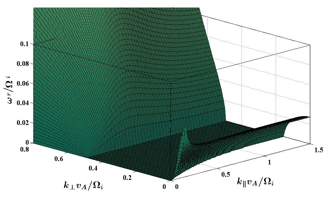
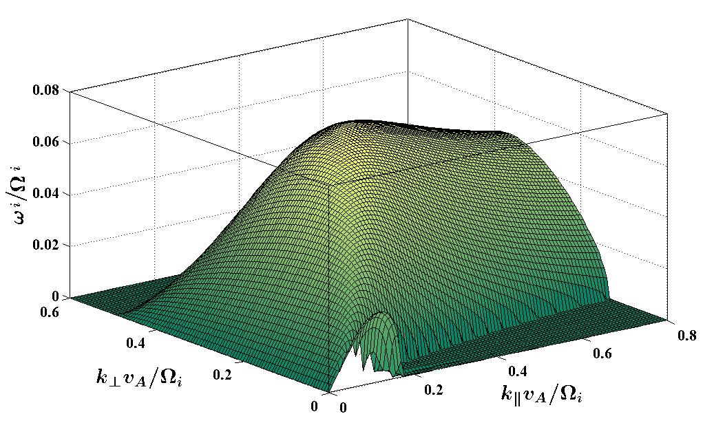
Figure 1: Plots of the real frequency (top panel) and of the growth rate (bottom panel) and of the unstable mode versus wave number for $\beta_{e}=2$ $\left(T_{\parallel e}=T_{\perp e}\right)$, $\beta_{\parallel i}=3$, $\beta_{\perp i}=0.8$ and $\kappa_{e}=\kappa_{i}=5$.

Figure 1 is similar to Fig. 4 of Yoon et al.(Yoon, Wu, and de Assis, 1993) In the bottom panel, one can observe that the growth rate of the instability is split in two branches: on the plane $k_{\perp}=0$ the instability is restricted to the range $0\leqslant k_{\parallel}v_{A}/\Omega_{i}\lesssim 0.16$. This branch rapidly vanishes as $k_{\perp}$ grows, while the other branch of the instability displays a growing behavior which climbs to a maximum $z_{i}\approx 0.07$ at $\left(q_{\parallel},q_{\perp}\right)\approx\left(0.37,0.32\right)$ and then gradually vanishes as well as $q_{\perp}$ grows, but falls slowly along the $q_{\parallel}$ direction. This branch of the instability was called the oblique firehose by Yoon et al.(Yoon, Wu, and de Assis, 1993) and the Alfvén firehose by Hellinger and Matsumoto.(Hellinger and Matsumoto, 2000) Another noticeable aspect is that the maximum growth rate of the oblique firehose is substantially larger than the maximum growth-rate of the parallel branch $\left(z_{i}\approx 0.02\right)$.

Over the spectral range where the oblique firehose is operative, one observes, in the top panel of figure 1, that the real part is zero; i.e., the oblique firehose instability occurs in a nonpropagating mode. This characteristic was pointed out by Refs. Yoon, Wu, and de Assis, 1993; Hellinger and Matsumoto, 2000 and is also valid for a kappa plasma.

The transition between the parallel and oblique branches of the instability can be seen in greater detail in figure 2, which is an inset of the bottom panel of figure 1. One can clearly observe the shooth transition between either branch of the instability, with the parallel branch confined in the range $0\leqslant q_{\perp}\lesssim 0.03$, $0\leqslant q_{\parallel}\lesssim 0.16$ and the oblique brach operative for $q_{\perp}\gtrsim 0.03$.

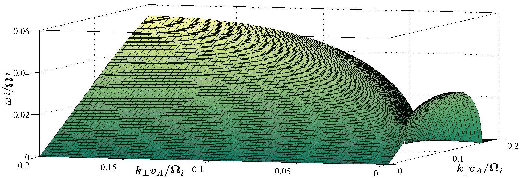
Figure 2: Transition between the parallel firehose instability and the oblique firehose. All other parameters as in Fig. 1.

The surface plots in figures 1 and 2 show the characteristics of the firehose instability for a single combination of electron/ion kappa parameters. If one wishes to analyze the dependency of the instability with different values for the kappas, 3D surface plots are not adequate. Instead, we will take the coordinates of the maximum growth rate for a Maxwellian plasma, which are $\left(q_{\parallel},q_{\perp}\right)\approx\left(0.41,0.37\right)$ for the parameters in figure 1, fix either $k_{\parallel}$ or $k_{\perp}$ and then plot the growth rates along the other component of the wave vector for several different values of $\kappa_{e}$, $\kappa_{i}$.

Proceeding in this way, we obtain the results shown in figure 3. In the present analysis, we will consider the particular choice of $\kappa_{e}=\kappa_{i}$. A more realistic and comprehensive analysis will be presented in a future publication. In the top panel of figure 3, we show the dependence of $\omega_{i}$ with $q_{\parallel}$ for a fixed $q_{\perp}=0.374$. The dashed curve is the solution of the Maxwellian limit of the dispersion equation (6), obtained directly from the expressions for a bi-Maxwellian VDF. The blue curve of Fig. 3(top), on the other hand, corresponds to the solution of (6) with $\kappa_{e}=\kappa_{i}=20$. As expected, this case is already close to the pure Maxwellian plasma environment. As the kappa indices decrease, the maximum growth rate along $q_{\parallel}$ also drops (from $z_{i,\mathrm{max}}\approx 0.08$ for $\kappa\to\infty$ to $z_{i,\mathrm{max}}\approx 0.062$ for $\kappa=3.5$), with the value of $q_{\parallel,\mathrm{max}}=0.41$ approximately the same for all kappas.

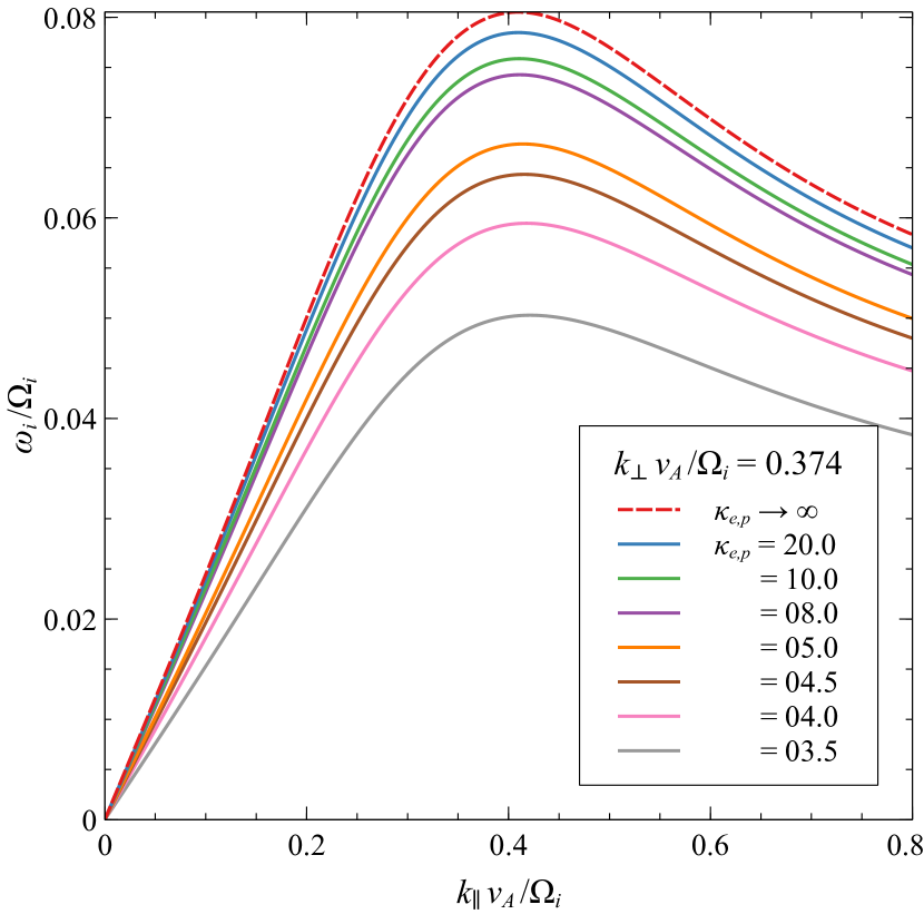
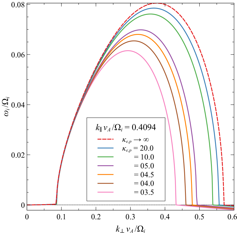
Figure 3: Plots of $\omega_{i}/\Omega_{i}$ for several values of $\kappa_{e}=\kappa_{i}$. Top panel: varying $k_{\parallel}$, keeping $q_{\perp}=0.374$ fixed. Bottom panel: varying $k_{\perp},$ keeping $q_{\parallel}=0.4094$ fixed. All other parameters are the same as in figure 1.

A different behavior is observed along $q_{\perp}$. The bottom panel of Fig. 3 again shows that the case $\kappa_{e}=\kappa_{i}=20$ is already close to the Maxwellian limit and that $z_{i,\mathrm{max}}$ drops as the kappas are reduced, with the same variation observed in the top panel. However, along the perpendicular direction one can observe some distinguishing features not aparent in the top panel. First of all, in the small $k_{\perp}$ region $\left(q_{\perp}\lesssim 0.17\right)$, corresponding to the “small gyroradius” case, the growth rate remains roughly independent of $\kappa$, with the limiting situation that at $q_{\perp}=0$ the solution is exactly the same as in the Maxwellian case. On the other hand, for $q_{\perp}\gtrsim 0.17$ the growth rate becomes dependent on $\kappa$, in such a way that not only the value of $z_{i,\mathrm{max}}$ reduces with $\kappa$, but the spectral range of the instability in the perpendicular direction reduces as well. Hence, these results suggest that for moderate values of the gyroradius, the oblique firehose instability is strongly dependant on the kappa parameter.

The same behavior is displayed by the real part of the unstable mode as a function of $k_{\perp}$, as can be seen in Figure 4. In the low gyroradious limit, the wave refracts as in a Maxwellian plasma, then the mode becomes nonpropagating throughout the unstable spectral range and finally becomes propagating again right at the point where the instability disapears and is replaced by damping. The value of $k_{\perp}$ where the mode ceases to be unstable is dependent on the kappa parameter, with the nonpropagating, unstable spectral range consistently reducing with $\kappa_{e}=\kappa_{i}$.

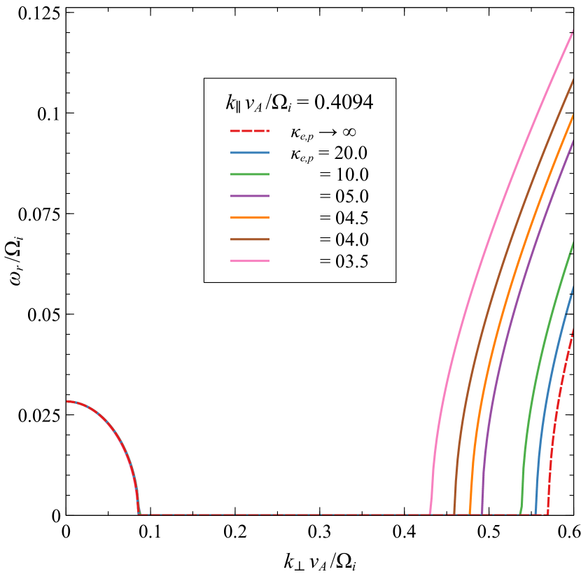
Figure 4: Plots of $\omega_{r}/\Omega_{i}$ for several values of $\kappa_{e}=\kappa_{i}$, varying $k_{\perp}$ with $q_{\parallel}=0.4094$ fixed. All other parameters are the same as in figure 1.

As a final result, figure 5 shows both the normalized growth rate (continuous lines) and the normalized real part (dotted lines) of the unstable mode for a fixed value of $q_{\parallel}$ and varying $q_{\perp}$. Now, the parallel component of the wavenumber is fixed to $k_{\parallel}v_{A}/\Omega_{i}=0.12$, which corresponds to the maximum growth rate of the (quasi) parallel branch of the firehose instability. The growth rates displayed by the figure clearly show the transition from the quasi-parallel to the oblique branches of the instability, which occurs at $q_{\perp}\approx 0.026$ for all values of the kappa parameter. We observe the same behavior displayed by Figs. 3 and 4: the quasi-parallel branch is almost independent on $\kappa_{e}$ and $\kappa_{i}$, whereas the oblique mode shows an evident dependence on the kappas. We again observe that not only the maximum growth rate is reduced with kappa, but so does also the unstable spectral range.

The real part of the unstable mode also repeats the same pattern observed in the previous figures: the quasi-parallel branch of the instability is convective, with nonzero phase velocity that is almost independent on the kappa values. On the other hand, the oblique branch is nonpropagating throughout the unstable spectral range and acquires a nonzero phase velocity when the instability disappears, being replaced by a very small damping coefficient.

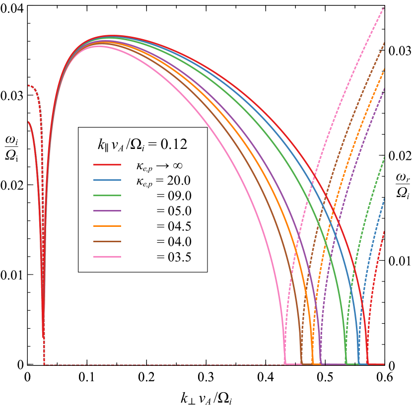
Figure 5: Plots of $\omega_{i}/\Omega_{i}$ (continuous lines) and $\omega_{r}/\Omega_{i}$ (dotted lines) as functions of $q_{\perp}$ for fixed $q_{\parallel}=0.12$ and various values of $\kappa_{e}=\kappa_{i}$. All other parameters as in Fig. 1.

As a final remark, we mention again that a more complete treatment will show that the quasi-parallel branch of the firehose instability does indeed depend on $\kappa_{i}$. However, this does not invalidate the present treatment, since the main objective was to study the effect of the superthermal nature of the electron and ion distribution functions on the oblique firehose instability, which does depend on the kappas.

V Conclusions

We presented the derivation of a dispersion equation that describes the oblique firehose instability excited in an electron-ion plasma depending on the wave vector, the parallel and perpendicular electron and ion beta parameters, and on the kappa parameters of the electron and ion velocity distribution functions.

In order to implement the numerical solution of the dispersion equation, several new mathematical properties of the kappa plasma special functions were obtained, which complement the formalism already derived in previous publications.

Employing values of the physical parameters that are relevant to space plasma conditions, some solutions of the dispersion equation were shown. The results show that both the maximum growth rate of the instability and its spectral range depend on the superthermal nature of the $\kappa$ distributions, with both properties roughly displaying a reduction with the values of $\kappa_{e}=\kappa_{i}$.

A more comprehensive and complete analysis of the oblique firehose instability was not reported here, due to the length of the paper demanded by the mathematical expressions. This task will be carried out in future publications, not only for the firehose instability but also for other relevant instabilities occurring in arbitrary angles, polarization and frequency ranges.