Analytical study of static beyond-Fröhlich Bose polarons in one dimension

Abstract

Grusdt et al. [New J. Phys. 19, 103035 (2017)] recently made a renormalization group study of a one-dimensional Bose polaron in cold atoms. Their study went beyond the usual Fröhlich description, which includes only single-phonon processes, by including two-phonon processes in which two phonons are simultaneously absorbed or emitted during impurity scattering [Shchadilova et. al., Phys. Rev. Lett. 117, 113002 (2016)]. We study this same beyond-Fröhlich model, but in the static impurity limit where the ground state is described by a multimode squeezed state instead of the multimode coherent state in the static Fröhlich model. We solve the system exactly by applying the generalized Bogoliubov transformation, an approach that can be straightforwardly adapted to higher dimensions. Using our exact solution, we obtain a polaron energy free of infrared divergences and construct analytically the polaron phase diagram. We find that the repulsive polaron is stable on the positive side of the impurity-boson interaction but is always thermodynamically unstable on the negative side of the impurity-boson interaction, featuring a bound state, whose binding energy we obtain analytically. We find that the attractive polaron is always dynamically unstable, featuring a pair of imaginary energies which we obtain analytically. We expect the multimode squeezed state to help with studies that go not only beyond the Fröhlich paradigm but also beyond Bogoliubov theory, just as the multimode coherent state has helped with the study of Fröhlich polarons.

I Introduction

An impurity submerged in a cold-atom Bose–Einstein condensate (BEC) represents an open quantum system. The concept of a Bose polaron emerges naturally in this system as an impurity dressed with phonons, where the phonons are low-energy excitations associated with density fluctuations of the BEC. That the impurity-phonon coupling in a BEC-polaron system may be modeled by terms linear in phonon fields makes the BEC-polaron system the cold-atom analog of the Fröhlich model for the electron-phonon system landau46ZhEkspTeorFiz.16.341 ; landau48ZhEkspTeorFiz.18.419 ; Fröhlich (1954). The Fröhlich paradigm has been quite influential in the study of many exciting phenomena, including high-temperature superconductivity in solid-state systems (see alexandrov07Book for a review). Of particular interest is the Fröhlich polaron in the regime with strong coupling between the impurity and phonons. In solid-state systems, the electron-phonon coupling is fixed by the underlying crystal structure. This limitation makes the Fröhlich polaron in the strong-coupling regime virtually inaccessible to solid-state experiments, despite extensive efforts in improving our theoretical understanding of such polarons landau46ZhEkspTeorFiz.16.341 ; landau48ZhEkspTeorFiz.18.419 ; Lee et al. (1953); Feynman (1955). In contrast, in cold-atom systems the impurity-phonon coupling can be made arbitrary large by tuning the interspecies interaction across a Feshbach resonance Chin et al. (2010). Cold atoms, then, are an excellent platform for exploring strongly interacting polarons (for recent reviews, see Devreese (2013); Grusdt and Demler (2015)). As such, there has been a flurry of theoretical Astrakharchik and Pitaevskii (2004); Cucchietti and Timmermans (2006); Kalas and Blume (2006); Bruderer et al. (2008); Huang and Wan (2009); Tempere et al. (2009); Casteels et al. (2011, 2012); Rath and Schmidt (2013); Kain and Ling (2014); Shashi et al. (2014); Li and Das Sarma (2014); grusdt15ScientificReports.5.12124 ; Ardila and Giorgini (2015); Vlietinck et al. (2015); Shchadilova et al. (2016a); Christensen et al. (2015); Ardila and Giorgini (2016); Levinsen et al. (2015); Kain and Ling (2016); Christensen et al. (2015); Levinsen et al. (2015); Dehkharghani et al. (2015); Ardila and Giorgini (2016); Kain and Ling (2016); Schmidt et al. (2016); Parisi and Giorgini (2017); Sun et al. (2017); Volosniev and Hammer (2017); Yoshida et al. (2018); arXiv:1807.09992 ; arXiv:1807.09948 and experimental Catani et al. (2012); Hu et al. (2016); Jørgensen et al. (2016); Meinert et al. (2017) activity devoted to the subject of Bose polarons in cold atoms.

Much of the theoretical work in recent years, however, has been done within the framework of the Fröhlich paradigm Tempere et al. (2009); Casteels et al. (2011, 2012); Vlietinck et al. (2015); grusdt15ScientificReports.5.12124 ; Shchadilova et al. (2016a); Kain and Ling (2016), and is therefore only valid when linearity is maintained in the phonon field operators for the impurity-phonon coupling. In crystal lattices, this linear relationship comes about because the electron’s potential energy is proportional to the displacement of ions from their equilibrium positions and effects from anharmonicity are usually negligible feynman90StatisticalMechanicsBook . In contrast, the linearity in atomic BECs comes about because of impurity scattering of bosons between the condensed and the noncondensed modes. However, the impurity can also scatter bosons just between noncondensed modes. As pointed out recently by Shchadilova et al. Shchadilova et al. (2016b), when the impurity-boson interaction is strong, an accurate description requires including such scattering, which, because both modes are to be treated quantum mechanically, introduces terms bilinear in phonon field operators, leading to a polaron model that goes beyond the Fröhlich paradigm Shchadilova et al. (2016b); Grusdt et al. (2017a, b).

Of special relevance to our work here is a recent paper by Grusdt et al. Grusdt et al. (2017b) on Bose polarons in one dimension, which analyzed the experiment by Catani et al. Catani et al. (2012) using a beyond-Fröhlich model where bosons are described within Bogoliubov theory. Despite the significant simplification afforded by Bogoliubov theory, as long as the impurity remains mobile, there is no known way to exactly solve the system (with arbitrary impurity-boson coupling and in the thermodynamic limit), be it modeled by the usual or the beyond-Fröhlich Hamiltonian. We base our study on the same model in the paper by Grusdt et al. Grusdt et al. (2017b), except we treat the impurity as static (i.e. localized in space). We carry out a field theoretical analysis of this static model, which is exactly solvable, irrespective of the impurity-phonon coupling strength. We expect such an exact treatment to offer insights that are valuable to ongoing efforts of constructing many-body field theoretic descriptions of (mobile) Bose polarons which go not only beyond the Fröhlich paradigm but also beyond Bogoliubov theory. (The term “polaron” is usually reserved for a dressed mobile impurity. Since the static impurity can be viewed as a mobile impurity in the heavy-mass limit, throughout this work we continue to use the same term for a dressed static impurity.)

Our paper is organized as follows. In Secs. II and III, we briefly review the model and mean-field solution. In Sec. IV, following a translation to displace phonon fields by their mean-field values, we apply the generalized Bogoliubov transformation to diagonalize (and hence solve exactly) the Hamiltonian associated with quantum fluctuations around the mean-field solution. It has been well established that observables in one-dimensional (1D) systems are plagued by infrared (IR) divergences which trace their origin to a dramatic increase in the density of states relative to its higher-dimensional counterparts. The polaron energy obtained using our exact solution is automatically free of the IR divergence that Grusdt et al. Grusdt et al. (2017b) managed to eliminate from the mean-field polaron energy using renormalization-group flow equations. In Sec. V, we investigate in detail the eigenvalues and corresponding eigenvectors of the Bogoliubov–de Gennes (BDG) equation for quantum fluctuations and construct the polaron phase diagram analytically. In agreement with Grusdt et al. Grusdt et al. (2017b), we find that the repulsive polaron on the attractive side of the impurity-boson interaction is distinguished by a bound state. Further, we obtain an analytical expression for the binding energy of this bound state. For the attractive polaron, quantum Monte Carlo simulations by Parisi and Giorgini Parisi and Giorgini (2017) suggest that for weak boson-boson repulsion, bosons may undergo an instability towards collapse around the impurity. For our static case, we show that the attractive polaron branch is always dynamically unstable within Bogoliubov theory and further we provide an analytical formula for determining the rate at which perturbations grow. We conclude our study in Sec. VI.

II Model and Hamiltonian

We consider a cold atom mixture with an extreme population imbalance where minority atoms are so outnumbered by majority atoms (bosons) that they can be considered impurities submerged in a bath of bosons. We assume that the two species have sufficiently different polarizabilities that impurities and host bosons can be independently manipulated by optical lattices. We specialize to the situation where one optical lattice traps and localizes impurities while another optical lattice confines host bosons to a quasi-1D geometry (a tube). In a nutshell, we base our theory on the experimental set-up described by Knap et al. Knap et al. (2012) in their investigation of the Anderson orthogonality catastrophe with the exception that 1D bosons instead of 3D fermions constitute the majority atoms.

We model this system, which describes potential scattering of bosons in one dimension, by the grand canonical Hamiltonian in momentum space,

$$\hat{H} =\sum_{\mathbf{k}}\left(\epsilon_{\mathbf{k}}-\mu\right)\hat{b}_{\mathbf{k}}^{\prime{\dagger}}\hat{b}_{\mathbf{k}}^{\prime}+\frac{g_{BB}}{2\mathcal{V}}\sum_{\mathbf{k},\mathbf{k}^{\prime}\mathbf{q}}\hat{b}_{\mathbf{k}+\mathbf{q}}^{\prime{\dagger}}\hat{b}_{\mathbf{k}^{\prime}-\mathbf{q}}^{\prime{\dagger}}\hat{b}_{\mathbf{k}^{\prime}}^{\prime}\hat{b}_{\mathbf{k}}^{\prime}$$

$$\qquad+\frac{g_{IB}}{\mathcal{V}}\sum_{\mathbf{k},\mathbf{k}^{\prime}}\hat{b}_{\mathbf{k}}^{\prime{\dagger}}\hat{b}_{\mathbf{k}^{\prime}}^{\prime},$$ (1)

where $\mathcal{V}$ is the quantization length and $\hat{b}_{\mathbf{k}}^{\prime}$ ($\hat{b}_{\mathbf{k}}^{\prime{\dagger}}$) is the field operator for annihilating (creating) a boson of mass $m_{B}$ with momentum $\mathbf{k}$ and energy $\epsilon_{\mathbf{k}}=k^{2}/2m_{B}$. The first line in Eq. (II) is the Hamiltonian for background bosons, with $\mu$ the chemical potential and $g_{BB}\left(>0\right)$ the effective 1D $s$-wave interaction strength between two bosons. The second line in Eq. (II) describes scattering between bosons and a localized impurity through a delta function potential with an effective 1D strength $g_{IB}$, which is fixed by the $s$-wave interaction between the impurity and a background boson.

Instead of $g_{IB}$ and $g_{BB}$, we may also measure two-body $s$-wave interactions with the corresponding effective 1D scattering lengths $a_{IB}$ and $a_{BB}$. In one dimension, a two-body delta potential with strength $g_{1D}$ can be shown to produce an $s$-wave scattering amplitude $f\left(k\right)=-1/\left(1+ika_{1D}\right)$, where $a_{1D}=-1/m_{r}g_{1D}$ and is defined as the 1D $s$-wave scattering length and $m_{r}$ is the reduced mass between two colliding particles Olshanii (1998). Thus, for the case of an infinitely heavy impurity, the two descriptions are related to each other according to

$$g_{BB}=\frac{-2}{m_{B}a_{BB}},\qquad g_{IB}=\frac{-1}{m_{B}a_{IB}}.$$ (2)

In cold-atom systems, effective 1D interaction strengths (and hence also their corresponding scattering lengths) can be tuned from negative to positive via confinement-induced resonance and are related to their 3D counterparts following well-established recipes, irrespective of whether the impurity and host bosons experience the same Olshanii (1998); Bergeman et al. (2003) or different Peano et al. (2005) trap frequencies.

As in our earlier publication Kain and Ling (2016), we limit our study to near zero temperatures where bosons are assumed to be in the deep BEC regime, i.e. there is a macroscopic occupation by bosons of the condensed ($\mathbf{k}=0$) mode. The Hohenberg-Mermin-Wagner theorem only prohibits infinite 1D Bose gases from forming a BEC Hohenberg (1967); Mermin and Wagner (1966), and thus does not apply to quasi-1D Bose gases in actual cold-atom experiments, which are neither strictly 1D nor infinite in size. By assuming the existence of a $\mathbf{k}=0$ BEC mode, we are, in essence, anticipating future applications of our theory to relatively large trapped gases in one dimension where true BECs exist at temperatures near zero Petrov et al. (2000).

In the spirit of the Bogoliubov approximation, we separate out the condensed mode $\mathbf{k}=0$, treating $\hat{b}_{\mathbf{0}}^{\prime}$ as the classical field ($c$-number) $b_{0}^{\prime}$, and replace the noncondensed fields $\hat{b}_{\mathbf{k}\neq 0}^{\prime}$ in favor of the phonon fields $\hat{b}_{\mathbf{k}}$ via the Bogoliubov transformation

$$\hat{b}_{\mathbf{k}}^{\prime}=u_{\mathbf{k}}\hat{b}_{\mathbf{k}}-v_{\mathbf{k}}\hat{b}_{-\mathbf{k}}^{{\dagger}},$$ (3)

where

$$u_{\mathbf{k}} =\sqrt{\frac{1}{2}\left(\frac{\epsilon_{\mathbf{k}}+g_{BB}n_{B}}{\omega_{\mathbf{k}}}+1\right)}$$ (4a)

$$v_{\mathbf{k}} =\sqrt{\frac{1}{2}\left(\frac{\epsilon_{\mathbf{k}}+g_{BB}n_{B}}{\omega_{\mathbf{k}}}-1\right)}$$ (4b)

and

$$\omega_{\mathbf{k}}=\sqrt{\epsilon_{\mathbf{k}}\left(\epsilon_{\mathbf{k}}+2g_{BB}n_{B}\right)}=v_{B}k\sqrt{1+\left(\xi_{B}k\right)^{2}},$$ (5)

where $v_{B}=\sqrt{n_{B}g_{BB}/m_{B}}$ is the phonon speed and

$$\xi_{B}=1/\sqrt{4m_{B}n_{B}g_{BB}}$$ (6)

is the healing length.

The Bogoliubov approximation divides the boson-boson interaction—the term associated with $g_{BB}$ in Eq. (II)—into two pieces that depend on whether or not the condensed bosons participate in the scattering process. The piece in which all scattering partners come from noncondensed modes (and is what Grusdt et al. Grusdt et al. (2017a, b) called the phonon-phonon interaction) is neglected in the Bogoliubov approach. As such, within Bogoliubov theory, the Bose gas can be approximated as consisting of a condensate with number (line) density $n_{B}=\left|b_{0}^{\prime}\right|^{2}/\mathcal{V}$ and chemical potential $\mu=n_{B}g_{BB}$, and a collection of noninteracting phonons that obey the dispersion spectrum $\omega_{\mathbf{k}}$ in Eq. (5). This description was shown to hold quite well by Lieb and Liniger (who solved the 1D Bose system exactly and analytically) in the weak-interacting regime, where the dimensionless coupling strength

$$\gamma\equiv\frac{m_{B}\left|g_{BB}\right|}{n_{B}}=\frac{2}{n_{B}\left|a_{BB}\right|}$$ (7)

is limited to $\gamma\leq 2$ Lieb and Liniger (1963); Lieb (1963). $\gamma$ in Eq. (7) is defined as the ratio of the interaction energy scale $n_{B}|g_{BB}|$ to the kinetic energy scale $n_{B}^{2}/m_{B}$ so that in one dimension, the lower the boson number density, the stronger the interaction. In the strong-interacting regime, where $\gamma>2$, an accurate description must go beyond the Bogoliubov theory by including phonon-phonon interactions Grusdt et al. (2017b).

Having separated out the condensed mode, we replace $\hat{b}_{\mathbf{k}}^{\prime}$ with the phonon field operator $\hat{b}_{\mathbf{k}}$ and change Hamiltonian (II) into Shchadilova et al. (2016b); Grusdt et al. (2017a, b)

$$\hat{H}=\hat{H}_{1}+\hat{H}_{2},$$ (8)

where

$$\hat{H}_{1} =n_{B}g_{IB}+\sum_{\mathbf{k}}\omega_{\mathbf{k}}\hat{b}_{\mathbf{k}}^{{\dagger}}\hat{b}_{\mathbf{k}}$$

$$\qquad+\frac{1}{\sqrt{\mathcal{V}}}\sum_{\mathbf{k}}g_{\mathbf{k}}\left(\hat{b}_{\mathbf{k}}+\hat{b}_{\mathbf{k}}^{{\dagger}}\right)$$ (9)

and

$$\hat{H}_{2} =\frac{g_{IB}}{\mathcal{V}}\sum_{\mathbf{k}}v_{\mathbf{k}}^{2}+\frac{1}{\mathcal{V}}\sum_{\mathbf{kk}^{\prime}}g_{\mathbf{kk}^{\prime}}^{+}\hat{b}_{\mathbf{k}}^{{\dagger}}\hat{b}_{\mathbf{k}^{\prime}}$$

$$\qquad+\frac{1}{2\mathcal{V}}\sum_{\mathbf{kk}^{\prime}}g_{\mathbf{kk}^{\prime}}^{-}\left(\hat{b}_{\mathbf{k}}^{{\dagger}}\hat{b}_{\mathbf{k}^{\prime}}^{{\dagger}}+\hat{b}_{\mathbf{k}}\hat{b}_{\mathbf{k}^{\prime}}\right),$$ (10)

with $g_{\mathbf{k}}$ and $g_{\mathbf{kk}^{\prime}}^{\pm}$ defined as

$$g_{\mathbf{k}} =g_{IB}\sqrt{n_{B}}\chi_{\mathbf{k}}$$ (11a)

$$g_{\mathbf{kk}^{\prime}}^{\pm} =\frac{g_{IB}}{2}\left(\chi_{\mathbf{k}}\chi_{\mathbf{k}^{\prime}}\pm\chi_{\mathbf{k}}^{-1}\chi_{\mathbf{k}^{\prime}}^{-1}\right),$$ (11b)

where

$$\chi_{\mathbf{k}}=\sqrt{\epsilon_{\mathbf{k}}/\omega_{\mathbf{k}}}.$$ (12)

$\hat{H}_{1}$ in Eq. (9) represents the usual Fröhlich Hamiltonian in the heavy impurity limit. The second line in Eq. (9), which is traced to impurity scattering of a boson from the condensed mode to a noncondensed mode, now represents single-phonon scattering. $\hat{H}_{2}$ in Eq. (10) represents the part that goes beyond the Fröhlich paradigm. The term $g_{IB}\sum_{\mathbf{k}}v_{\mathbf{k}}^{2}/\mathcal{V}$ arises from normal ordering. The remaining terms in Eq. (10) describe two-phonon scattering, which is traced to impurity scattering of a boson between two noncondensed modes and is therefore important in the limit of strong impurity-boson interactions.

III Mean-Field Solution

In the absence of $H_{2}$, $\hat{H}=\hat{H}_{1}$ in Eq. (9), which has the same mathematical form as the electron-phonon Hamiltonian when the electrons are localized in space. This Hamiltonian is known to have the exact solution Mahan00Book

$$\left|z\right\rangle={\displaystyle\prod\limits_{\mathbf{k}}}\left|z_{\mathbf{k}}\right\rangle,$$ (13)

where

$$\left|z_{\mathbf{k}}\right\rangle=\exp\left(z_{\mathbf{k}}\hat{b}_{\mathbf{k}}^{{\dagger}}-z_{\mathbf{k}}^{\ast}\hat{b}_{\mathbf{k}}\right)\left|0\right\rangle$$ (14)

is the coherent state of mode k and $z_{\mathbf{k}}=-g_{\mathbf{k}}/(\omega_{\mathbf{k}}\sqrt{\mathcal{V}})$. The mean-field variational approach Lee et al. (1953); Shashi et al. (2014); Shchadilova et al. (2016b) amounts to assuming that even when $H_{2}$ is included, the ground state continues to be in the product state (13), but with $z_{\mathbf{k}}$ a variational parameter to be determined. The expectation value of the Hamiltonian in the coherent state is

$$\mathcal{E}\left(z,z^{\ast}\right)=\left\langle z\right|\hat{H}(\hat{b},\hat{b}^{{\dagger}})\left|z\right\rangle=\hat{H}(z,z^{\ast}),$$ (15)

where in the second equality we used that $\hat{H}(\hat{b},\hat{b}^{{\dagger}})$ in Eqs. (9) and (10) is in a normally ordered form. Minimizing the energy $\mathcal{E}(z,z^{*})$ with respect to $z_{\mathbf{k}}$ leads to the saddle point equation

$$\omega_{\mathbf{k}}z_{\mathbf{k}}+\frac{\chi_{\mathbf{k}}}{\mathcal{V}}g_{IB}\sum_{\mathbf{k}^{\prime}}\chi_{\mathbf{k}^{\prime}}z_{\mathbf{k}^{\prime}}=-\frac{g_{\mathbf{k}}}{\sqrt{\mathcal{V}}}.$$ (16)

In arriving at Eq. (16), we have taken $z_{\mathbf{k}}$ to be purely real because the coupling constant $g_{\mathbf{k}}$ is a real number. The mean-field polaron energy, defined as $\mathcal{E}_{0}\equiv\mathcal{E}\left(z,z^{\ast}\right)$ at the saddle point, simplifies to

$$\mathcal{E}_{0}=n_{B}g_{IB}+\frac{1}{\sqrt{\mathcal{V}}}\sum_{\mathbf{k}}g_{\mathbf{k}}z_{\mathbf{k}}+\frac{g_{IB}}{\mathcal{V}}\sum_{\mathbf{k}}v_{\mathbf{k}}^{2}.$$ (17)

When $z_{\mathbf{k}}$ in Eq. (17) is replaced with the solution to Eq. (16),

$$z_{\mathbf{k}}=-\frac{1}{\sqrt{\mathcal{V}}}\frac{g_{\mathbf{k}}/\omega_{\mathbf{k}}}{1+\frac{g_{IB}}{\mathcal{V}}\sum_{\mathbf{k}}\frac{\chi_{\mathbf{k}}^{2}}{\omega_{\mathbf{k}}}},$$ (18)

the mean-field polaron energy takes its final form,

$$\mathcal{E}_{0}=\mathcal{E}_{0}^{M}+\frac{g_{IB}}{\mathcal{V}}\sum_{\mathbf{k}}v_{\mathbf{k}}^{2},$$ (19)

where

$$\mathcal{E}_{0}^{M}\equiv\frac{n_{B}}{\frac{1}{g_{IB}}+\frac{1}{\mathcal{V}}\sum_{\mathbf{k}}\frac{\chi_{\mathbf{k}}^{2}}{\omega_{\mathbf{k}}}}.$$ (20)

The last term, $g_{IB}\sum_{\mathbf{k}}v_{\mathbf{k}}^{2}/\mathcal{V}$, arises from the normal ordering of $\hat{H}_{2}$ in Eq. (10) and thus represents vacuum energy contributed by quantum fluctuations associated with the interaction between the impurity and noncondensed bosons. In the infrared limit, where the low-momentum cutoff, $\lambda$, approaches zero, the term $g_{IB}\sum_{\mathbf{k}}v_{\mathbf{k}}^{2}/\mathcal{V}$ diverges with $\lambda$ logarithmically as $-g_{IB}\sqrt{m_{B}n_{B}g_{BB}}\left(\ln\lambda\right)/2\pi$. This log-divergence can be traced to the 1D density of states being inversely proportional to the square root of the energy, leading to a dramatic enhancement of quantum fluctuations in the IR limit. This same enhancement was at the heart of the Hohenberg-Mermin-Wagner theorem Hohenberg (1967); Mermin and Wagner (1966), which precludes a true BEC from forming in a true 1D infinite Bose system. Following Grusdt et al. Grusdt et al. (2017b), we remove the divergent term from $\mathcal{E}_{0}$, treating $\mathcal{E}_{0}^{M}$ as “the polaron energy in the mean-field theory.” The quotation marks are meant to indicate that $\mathcal{E}_{0}^{M}$, obtained in such a brute-force manner, should not be regarded as the result of a consistent theory. That it agrees well with the exact result, which is presented in the next section, means only that $\mathcal{E}_{0}^{M}$ may serve as a good measuring stick for our exact theory.

IV Exact Solution

In this section, we solve $\hat{H}$ exactly and obtain a polaron energy free of the IR divergence. We start by replacing the phonon field operators $\hat{b}_{\mathbf{k}}$ and $\hat{b}_{\mathbf{k}}^{{\dagger}}$ with the shifted phonon field operators

$$\hat{c}_{\mathbf{k}} =\hat{b}_{\mathbf{k}}-z_{\mathbf{k}}$$ (21a)

$$\hat{c}_{\mathbf{k}}^{{\dagger}} =\hat{b}_{\mathbf{k}}^{{\dagger}}-z_{\mathbf{k}}^{\ast},$$ (21b)

which describe quantum fluctuations around $$z_{\mathbf{k}} \hat{c}_{\mathbf{k}} \hat{c}_{\mathbf{k}}^{{\dagger}}$$, the saddle-point solution in Eq. (18). By virtue of the saddle-point condition in Eq. (16), the Hamiltonian in terms of the shifted operators is free of the Fröhlich terms (those linear in and ) and is given by

$$\hat{H} =\mathcal{E}_{0}+\sum_{\mathbf{k}}\omega_{\mathbf{k}}\hat{c}_{\mathbf{k}}^{{\dagger}}\hat{c}_{\mathbf{k}}+\frac{1}{\mathcal{V}}\sum_{\mathbf{kk}^{\prime}}g_{\mathbf{kk}^{\prime}}^{+}\hat{c}_{\mathbf{k}}^{{\dagger}}\hat{c}_{\mathbf{k}^{\prime}}$$

$$\qquad+\frac{1}{2\mathcal{V}}\sum_{\mathbf{kk}^{\prime}}g_{\mathbf{kk}^{\prime}}^{-}\left(\hat{c}_{\mathbf{k}}^{{\dagger}}\hat{c}_{\mathbf{k}^{\prime}}^{{\dagger}}+\hat{c}_{\mathbf{k}}\hat{c}_{\mathbf{k}^{\prime}}\right),$$ (22)

which is quadratic and is therefore exactly solvable.

Following the standard procedure, we introduce the quasiparticle field operator $\hat{d}_{n}$ through the generalized Bogoliubov transformation

$$\hat{d}_{n} =\sum_{\mathbf{k}}\left(U_{n\mathbf{k}}^{\ast}\hat{c}_{\mathbf{k}}-V_{n\mathbf{k}}^{\ast}\hat{c}_{\mathbf{k}}^{{\dagger}}\right)$$ (23a)

$$\hat{d}_{n}^{{\dagger}} =\sum_{\mathbf{k}}\left(U_{n\mathbf{k}}\hat{c}_{\mathbf{k}}^{{\dagger}}-V_{n\mathbf{k}}\hat{c}_{\mathbf{k}}\right),$$ (23b)

where $$U V \mathcal{N}\times\mathcal{N} \mathcal{N} \mathbf{k} n U V n \left(U_{n},V_{n}\right)^{T}$$ and are matrices, with being the total number of modes in momentum space. The th row of the and matrices contains the th eigenstate, , of the eigenvalue equation

$$M\left(\begin{array}[c]{c}U_{n}\\ V_{n}\end{array}\right)=w_{n}\left(\begin{array}[c]{c}U_{n}\\ V_{n}\end{array}\right),$$ (24)

where $M$ is the $2\mathcal{N}\times 2\mathcal{N}$ matrix

$$M\equiv\left(\begin{array}[c]{cc}A&B\\ -B&-A\end{array}\right),$$ (25)

with $A$ and $B$ being the $\mathcal{N}\times\mathcal{N}$ matrices, whose components are

$$A_{\mathbf{kk}^{\prime}} =\omega_{\mathbf{k}}\delta_{\mathbf{k},\mathbf{k}^{\prime}}+\frac{g_{\mathbf{kk}^{\prime}}^{+}}{\mathcal{V}}$$ (26)

$$B_{\mathbf{kk}^{\prime}} =\frac{g_{\mathbf{kk}^{\prime}}^{-}}{\mathcal{V}}.$$ (27)

Note that the generalized Bogoliubov transformation (23) mixes annihilation and creation operators in exactly the same manner as the multimode squeezing operator in quantum optics walls08Book . In the beyond-Fröhlich model, squeezing is traced to simultaneous creation or annihilation of two noncondensed bosons by impurity scattering, which are nonlinear matter wave mixing processes akin to parametric up and down conversion of light waves, which are responsible for the squeezing phenomenon in quantum optics.

If all eigenvalues are real, we can cast Hamiltonian (22) into the diagonal form

$$\hat{H} =\mathcal{E}_{0}^{M}+\sum_{n}w_{n}\hat{d}_{n}^{{\dagger}}\hat{d}_{n}+\frac{1}{2}\left(\sum_{n}w_{n}-\sum_{\mathbf{k}}\omega_{\mathbf{k}}\right)$$

$$\qquad+\frac{g_{IB}}{\mathcal{V}}\sum_{\mathbf{k}}v_{\mathbf{k}}^{2}-\frac{1}{2}\sum_{\mathbf{k}}\frac{g_{\mathbf{kk}}^{+}}{\mathcal{V}},$$ (28)

which is in terms of $\hat{d}_{n}$, where the sum over $n$ is only over eigenstates $\left|w_{n}\right\rangle$ with positive norm $\left\langle w_{n}\right|\zeta\left|w_{n}\right\rangle>0$, where $\zeta$ is the $2\mathcal{N}\times 2\mathcal{N}$ matrix

$$\zeta=\left(\begin{array}[c]{cc}I&0\\ 0&-I\end{array}\right),$$ (29)

with $I$ the $\mathcal{N}\times\mathcal{N}$ identity matrix. In other words, the sum over $n$ includes only those eigenmodes which can be normalized to +1 with metric $\zeta$:

$$\left\langle w_{n}\right|\zeta\left|w_{n}\right\rangle=1,$$ (30)

or explicitly

$$\sum_{\mathbf{k}}\left(\left|U_{n\mathbf{k}}\right|^{2}-\left|V_{n\mathbf{k}}\right|^{2}\right)=1.$$ (31)

The fact that $\hat{H}$ in Eq. (22) is exactly solvable by the generalized Bogoliubov transformation means that the ground polaron state for the beyond-Fröhlich model is an exact multimode squeezing state.

Equation (24) is the bosonic analog of the Bogoliubov–de Gennes (BDG) equation for fermions in the state of superfluid pairings. In contrast to the matrix in the BDG equation for fermions, which is Hermitian, the matrix $M$ in the BDG equation for bosons [Eq. (24)] is non-Hermitian and its eigenvalues can be complex. Just as there exists an intrinsic anti-unitary particle-hole symmetry in the fermionic BDG Hasan and Kane (2010), there exists, in the bosonic BDG equation (24), an analogous built-in symmetry:

$$\tau M\tau^{-1}=-M,$$ (32)

which maps $M$ to $-M$, with $\tau$ being the orthogonal matrix

$$\tau=\left(\begin{array}[c]{cc}0&I\\ I&0\end{array}\right).$$ (33)

As a consequence of this “particle-hole” symmetry, for every eigenvector $\left|w_{n}\right\rangle=\left(U_{n},V_{n}\right)^{T}$ with a nonvanishing eigenvalue $w_{n}$, there corresponds an eigenvector

$$\left|-w_{n}\right\rangle=\tau\left|w_{n}\right\rangle=\left(V_{n},U_{n}\right)^{T}$$ (34)

with an eigenvalue $-w_{n}$. Eigenvalues in our system therefore appear in pairs with opposite signs

Thus, there arise three possible scenarios for stability of the system. (a) The system is said to be dynamically unstable if one or more pairs of eigenvalues are complex—an exponentially small perturbation can cause the system to depart irreversibly from equilibrium. In the absence of any pairs of complex eigenvalues, (b) the system is said to be thermodynamically unstable if one or more eigenvalues associated with eigenvectors normalizable to $+1$ with metric $\zeta$ are negative—such a state cannot be created adiabatically by gradually reducing the entropy associated with the thermal energy—and (c) the system is said to be thermodynamically stable if all eigenvalues associated with eigenvectors normalized to $+1$ with metric $\zeta$ are positive.

In cases (b) and (c), i.e. those without complex eigenvalues, Eq. (28) holds true. We are thus led to define

$$E_{0}=\mathcal{E}_{0}^{M}+\frac{1}{2}\left(\sum_{n}w_{n}-\sum_{\mathbf{k}}\omega_{\mathbf{k}}\right)-\frac{g_{IB}}{2\mathcal{V}}\sum_{\mathbf{k}}$$ (35)

as the polaron energy in a metastable state for case (b) and the polaron energy in the ground state for case (c).

In case (a), Eq. (28) does not apply because modes with complex eigenvalues arise. Such modes always have a vanishing norm with respect to metric $\zeta$ and are therefore excluded from Eq. (35), where the sum is limited only to modes normalizable to $+1$ with metric $\zeta$. Thus, for case (a), Eq. (35), in fact, is well defined. In the present study, we continue to use Eq. (35) as the “polaron energy” for case (a). For a polaron system where complex eigenvalues are all purely imaginary, Eq. (35) gives the exact polaron energy in the limit of vanishingly small imaginary eigenvalues. In this situation, for all practical purposes, the polaron can be considered as dynamically stable. Since in our system, complex eigenvalues are purely imaginary and have small imaginary parts (as we discuss in the next section), the use of Eq. (35) for the polaron energy is not particularly unreasonable.

A comment is in order concerning IR and ultraviolet (UV) divergences. The last term in Eq. (28), when making use of $g_{\mathbf{kk}}^{+}$ in Eq. (11b) and $v_{\mathbf{k}}$ in Eq. (4b), becomes

$$\frac{1}{2}\sum_{\mathbf{k}}\frac{g_{\mathbf{kk}}^{+}}{\mathcal{V}}=\frac{g_{IB}}{\mathcal{V}}\sum_{\mathbf{k}}v_{\mathbf{k}}^{2}+\frac{g_{IB}}{2\mathcal{V}}\sum_{\mathbf{k}},$$ (36)

which is found to contain an identical IR divergence term $g_{IB}\sum_{\mathbf{k}}v_{\mathbf{k}}^{2}/\mathcal{V}$. This explains how the sum of the last two terms in Eq. (28) eliminates the IR divergence, but it gives rise to a UV divergence represented by the last term in Eq. (35). The middle term in Eq. (35) (which in a Fermi polaron system Kain and Ling (2017) is finite because of the Fermi surface) is found (numerically) to contain a UV divergence that is identical and therefore cancels the UV divergent term in Eq. (35). In conclusion, the polaron energy in one dimension, when quantum fluctuations are taken care of exactly, are free of both IR and UV divergences.

Figure 1 compares, within the weakly (Bose-Bose) interacting regime, the exact polaron energy $E_{0}$ (solid black curves), given by Eq. (35), with the mean-field polaron energy $\mathcal{E}_{0}^{M}$ (dashed blue curves), given by Eq. (20). The energies are given as a function of $\eta$, where $\eta$ is the dimensionless parameter

$$\eta=\frac{g_{IB}}{g_{BB}},$$ (37)

which measures the impurity-boson interaction relative to the boson-boson interaction. For $\eta>0$, the polaron is repulsive and the energy increases with $\eta$ monotonically from 0 until it saturates in the limit of large positive $\eta$. For $\eta<0$, the polaron changes from attractive to repulsive as $\eta$ decreases across a critical value,

$$\eta_{c}=-2/\sqrt{\gamma},$$ (38)

at which the denominator in $\mathcal{E}_{0}^{M}$ [Eq. (20)] vanishes, the details of which we present in the next section. When the polaron energy is plotted as a function of $\eta^{-1}$, it becomes evident that the two branches of repulsive polarons, which are separated in $\eta$ space, are actually adiabatically connected—there is a smooth crossover when $\eta^{-1}$ changes across $0$ (unitarity).

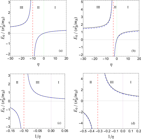
Figure 1: The top row displays the polaron energy as a function of $\eta=g_{IB}/g_{BB}$ and the bottom row as a function of $1/\eta$. The exact polaron energy, $E_{0}$, is represented by solid black curves and the mean field polaron energy, $\mathcal{E}_{0}^{M}$, by dashed blue curves. The left column, (a) and (c), has $\gamma=0.04$ and the right column, (b) and (d), has $\gamma=0.4$. The dashed red line marks the critical value $\eta_{c}=-2/\sqrt{\gamma}$. In each plot I, II, and III indicate phases, which are explained in Sec. V and in the caption to Fig. 2.

It can be seen that quantum fluctuations, which are absent in the mean-field approach, offset almost entirely the IR-divergent term in $\mathcal{E}_{0}$, the last term in Eq. (19), so that the exact polaron energy $E_{0}$ remains fairly close to $\mathcal{E}_{0}^{M}$. That the two results are very close to each other, even in the limit of large $\left|\eta\right|$, is expected to be the case only in the limit of an infinitely heavy impurity. For a mobile impurity, impurity recoil contributes additional terms to the Hamiltonian that are inversely proportional to the impurity mass. As the impurity becomes lighter, $E_{0}$ is expected to become increasingly different from $\mathcal{E}_{0}^{M}$, especially in the strong-coupling regime where $\left|\eta\right|$ is large Grusdt et al. (2017b).

V Eigenvalue Analysis and Exact Phase Diagrams

We can gain significant insight into the stability of the system by analyzing the eigenvalue matrix equation. We now work to solve the eigenvalue and eigenvector problem from the coupled equations. (In this section, when no confusion is likely to arise, we drop the subscript $n$ and write $w_{n},U_{n\mathbf{k}}$, and $V_{n\mathbf{k}}$ as $w,U_{\mathbf{k}}$, and $V_{\mathbf{k}}$ for notational simplicity.) We first define, for each $\mathbf{k}$, the two variables $X_{\mathbf{k}}^{\pm}$ as

$$\left(\begin{array}[c]{c}X_{\mathbf{k}}^{+}\\ X_{\mathbf{k}}^{-}\end{array}\right)=\frac{1}{2}\left(\begin{array}[c]{cc}1&1\\ 1&-1\end{array}\right)\left(\begin{array}[c]{c}U_{\mathbf{k}}\\ V_{\mathbf{k}}\end{array}\right)$$ (39)

and transform Eq. (24) into

$$\left(\begin{array}[c]{c}X_{\mathbf{k}}^{+}\\ X_{\mathbf{k}}^{-}\end{array}\right)=\frac{g_{IB}}{\mathcal{V}}\left(\begin{array}[c]{c}\frac{\chi_{\mathbf{k}}\omega_{\mathbf{k}}}{w^{2}-\omega_{\mathbf{k}}^{2}},\frac{\chi_{\mathbf{k}}^{-1}w}{w^{2}-\omega_{\mathbf{k}}^{2}}\\ \frac{\chi_{\mathbf{k}}w}{w^{2}-\omega_{\mathbf{k}}^{2}},\frac{\chi_{\mathbf{k}}^{-1}\omega_{\mathbf{k}}}{w^{2}-\omega_{\mathbf{k}}^{2}}\end{array}\right)\left(\begin{array}[c]{c}a^{+}\\ a^{-}\end{array}\right),$$ (40)

where $a^{\pm}$ are constants defined as

$$a^{+}=\sum_{\mathbf{k}}\chi_{\mathbf{k}}X_{\mathbf{k}}^{+},\qquad a^{-}=\sum_{\mathbf{k}}\chi_{\mathbf{k}}^{-1}X_{\mathbf{k}}^{-}.$$ (41)

This leads to the following linearly coupled homogeneous equations for $a^{\pm}$:

$$\left(\begin{array}[c]{cc}g_{IB}^{-1}+I_{+}\left(w^{2}\right)&wI_{0}\left(w^{2}\right)\\ wI_{0}\left(w^{2}\right)&g_{IB}^{-1}+I_{-}\left(w^{2}\right)\end{array}\right)\left(\begin{array}[c]{c}a^{+}\\ a^{-}\end{array}\right)=0,$$ (42)

where

$$I_{0}\left(x\right) =\frac{1}{\mathcal{V}}\sum_{\mathbf{k}}\frac{1}{\omega_{\mathbf{k}}^{2}-x},$$ (43a)

$$I_{\pm}\left(x\right) =\frac{1}{\mathcal{V}}\sum_{\mathbf{k}}\frac{\chi_{\mathbf{k}}^{\pm 2}\omega_{\mathbf{k}}}{\omega_{\mathbf{k}}^{2}-x}.$$ (43b)

The eigenvalues follow from the vanishing of the determinant, and thus are the roots of the equation

$$F\left(w^{2}\right) \equiv-w^{2}\left[I_{0}\left(w^{2}\right)\right]^{2}$$

$$\qquad+\left[g_{IB}^{-1}+I_{+}\left(w^{2}\right)\right]\left[g_{IB}^{-1}+I_{-}\left(w^{2}\right)\right].$$ (44)

The corresponding eigenvectors are given by

$$U_{\mathbf{k}} =\frac{\chi_{\mathbf{k}}}{w-\omega_{\mathbf{k}}}\frac{f}{\sqrt{\mathcal{V}}}\left[1-\frac{g_{IB}^{-1}+I_{+}\left(w^{2}\right)}{w\chi_{\mathbf{k}}^{2}I_{0}\left(w^{2}\right)}\right]$$ (45a)

$$V_{\mathbf{k}} =\frac{-\chi_{\mathbf{k}}}{w+\omega_{\mathbf{k}}}\frac{f}{\sqrt{\mathcal{V}}}\left[1+\frac{g_{IB}^{-1}+I_{+}\left(w^{2}\right)}{w\chi_{\mathbf{k}}^{2}I_{0}\left(w^{2}\right)}\right],$$ (45b)

where $$f$$ is determined by the normalization condition (31).

The system is dynamically unstable if $w$ is a complex number. For our system, when complex eigenvalues occur, numerical simulations suggest that there exists no more than a single pair. Then, the complex eigenvalues must be purely imaginary, as we explain. In addition to the “particle-hole” symmetry (32), our BDG equation has the time-reversal symmetry

$$KMK^{-1}=M,$$ (46)

where $K$ is the complex conjugate operation. This implies that for every eigenvector $\left|w_{n}\right\rangle=(U_{n},V_{n})^{T}$ with nonvanishing eigenvalue $w_{n}$, there exists an eigenvector

$$\left|w_{n}^{\ast}\right\rangle=K\left|w_{n}\right\rangle=\left(U_{n}^{\ast},V_{n}^{\ast}\right)^{T}$$ (47)

with eigenvalue $w_{n}^{*}$. In consequence, for a complex eigenvalue $w_{n}$, in addition to the pair $w_{n}$ and $-w_{n}$ guaranteed by the “particle-hole” symmetry, there exists another pair, $w_{n}^{\ast}$ and $-w_{n}^{\ast}$, guaranteed by the time-reversal symmetry. For real eigenvalues the second pair is redundant, since it is identical to the first pair. For complex eigenvalues, however, only when they are purely imaginary are the two pairs equivalent. Thus, in our case where among all pairs of eigenvalues, only one pair is complex, complex eigenvalues must be purely imaginary.

As a result, our system makes a transition from thermodynamically stable or metastable to dynamically unstable when $w^{2}$ changes from positive to negative, which obviously occurs at $w^{2}=0$. Since Eq. (44) must be satisfied, we have for $w^{2}=0$ either

$$\frac{1}{g_{IB}}+\frac{1}{\mathcal{V}}\sum_{\mathbf{k}}\frac{\chi_{\mathbf{k}}^{-2}}{\omega_{\mathbf{k}}}=0$$ (48)

or

$$\frac{1}{g_{IB}}+\frac{1}{\mathcal{V}}\sum_{\mathbf{k}}\frac{\chi_{\mathbf{k}}^{2}}{\omega_{\mathbf{k}}}=0.$$ (49)

The first possibility (48) can be shown to be satisfied when

$$g_{IB}=0,$$ (50)

(more precisely, $g_{IB}=0^{-}$), which is expected to be unique to one dimension, since in arriving at it, we made explicit use of the IR divergence—the sum in Eq. (48) equals $m_{B}/\pi\lambda$ in the continuous limit and hence diverges in the IR limit when $\lambda\rightarrow 0^{+}$. The second condition (49) coincides with the mean-field singularity, where the polaron changes from attractive to repulsive (as mentioned in the previous section), and is equivalent to

$$g_{IB}=g_{c}\equiv-\sqrt{\frac{4n_{B}g_{BB}}{m_{B}}}.$$ (51)

Since$\ g_{IB}$ in one dimension has dimensions of energy $\times$ length, we define

$$\bar{g}_{IB}=\frac{g_{IB}}{1/(m_{B}\xi_{B})}$$ (52)

as a unitless parameter that measures the impurity-boson $s$-wave interaction in units of $1/m_{B}\xi_{B}$, where $\xi_{B}$ is the healing length defined in Eq. (6). The second critical condition (51) is then simply

$$\bar{g}_{IB}=\bar{g}_{c}\equiv-1.$$ (53)

Thus, the $\bar{g}_{IB}$-phase diagram is very simple. It is divided into phase I, where $\bar{g}_{IB}>0$; phase II, where $-1<\bar{g}_{IB}<0$; and phase III, where $\bar{g}_{IB}<-1$. Further, $\bar{g}_{IB}$ is related to $\gamma$ (${>0}$) in Eq. (7) and $\eta$ in Eq. (37) according to

$$\bar{g}_{IB}=\eta\sqrt{\gamma}/2.$$ (54)

As a result, for the $(\eta,\gamma)$-phase diagram, the three segments in the $\bar{g}_{IB}$-phase diagram morph into three areas bordered by $\eta\sqrt{\gamma}=-2,\eta=0$, and $\gamma=0$. The $\bar{g}_{IB}$- and $(\eta,\gamma)$-phase diagrams are shown in Fig. 2.

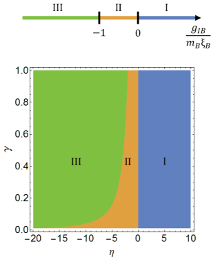
Figure 2: The three phases of our system: thermodynamically stable (phase I), dynamically unstable (phase II), and thermodynamically unstable (phase III). The phase diagram at the top indicates where these phases occur in the one-dimensional $g_{IB}$-parameter space. The bottom phase diagram equivalently indicates where these phases occur in the two-dimensional $(\eta,\gamma)$-parameter space.

We now examine $F(w^{2})$ in Eq. (44) and solve for its roots, i.e. the solutions to $F(w^{2})=0$, which allows us to determine the stability properties of the three phases in the phase diagrams. Figure 3 plots $F(w^{2})$ as a function of $w^{2}$. We find that the function contains poles that are regularly spaced at the locations of $\omega_{\mathbf{k}}^{2}$ with a single root trapped between adjacent poles. We refer to these as “regular” roots. The totality of the regular roots when converted to energy forms the continuum part of the eigenenergy spectrum. Figure 3(a) illustrates a typical $F(w^{2})$ in phase I (of the phase diagrams), in which every root is a regular one sandwiched between adjacent poles. Figures 3(c) and 3(e) illustrate a typical $F(w^{2})$ in phases II and III, respectively. In phase II, in addition to the regular roots, there emerges an isolated root that lies at $w^{2}<0$, but close to the origin. In phase III, $F(w^{2})$ again maintains the same pattern with respect to the regular roots, but now also contains one additional $w^{2}>0$ root, where two roots lie between adjacent poles. In the continuum $\mathbf{k}$ limit, one of the two roots joins the continuum while the other one becomes part of the discrete spectrum.

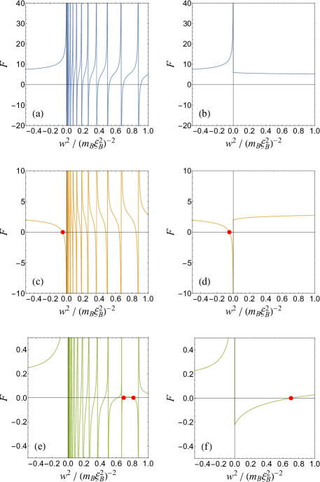
Figure 3: Each row displays the function $F(w^{2})$, given in Eq. (44), as a function of $w^{2}$ for one of the three phases. The roots of $F(w^{2})$, i.e. the points at which it crosses the horizontal axis, are the square of the eigenenergies, $w_{n}^{2}$, of the eigenvalue equation (24). In all plots $\gamma=0.04$. The left column displays $F(w^{2})$ as computed with the discrete sums in Eqs. (43) and the right column displays $F(w^{2})$ in the continuous limit where the discrete sums are replaced with integrals with respect to momentum. By comparing the left column with the right, we can see how discrete roots survive in the continuous limit. The top row, (a) and (b), displays phase I with $\bar{g}_{IB}=g_{IB}/(m_{B}\xi_{B})^{-1}=0.5$ (equivalently $\eta=5$), the middle row, (c) and (d), displays phase II with $\bar{g}_{IB}=-0.5$ ($\eta=-5$), and the bottom row, (e) and (f), displays phase III with $\bar{g}_{IB}=-1.5$ ($\eta=-15$).

We can determine the discrete spectrum by moving to the continuous $\mathbf{k}$ limit by converting discrete sums over $\mathbf{k}$ in Eq. (43) to integrals over $\mathbf{k}$, which can be evaluated analytically. We arrive at the results

$$I_{n=0,\pm}\left(x\right)=\left\{\begin{array}[c]{c}I_{n}^{>}\left(x\right)\text{, if }x>0\\ I_{n}^{<}\left(x\right)\text{, if }x<0\end{array}\right.\text{, }$$ (55)

where

$$I_{\pm}^{>}\left(x\right) =\left(-\sqrt{b^{2}+x}\mp b\right)I_{0}^{>}\left(x\right),$$ (56a)

$$I_{0}^{>}\left(x\right) =\frac{-\sqrt{m_{B}/8}}{\sqrt{b^{2}+x}\sqrt{b+\sqrt{b^{2}+x}}},$$ (56b)

and

$$I_{\pm}^{<}\left(x\right) =\left[\sqrt{-x}+\left(1\mp 1\right)b\right]I_{0}^{<}\left(x\right),$$ (57a)

$$I_{0}^{<}\left(x\right) =\frac{\sqrt{b+\sqrt{b^{2}+x}}-\sqrt{b-\sqrt{b^{2}+x}}}{\sqrt{8/m_{B}}\sqrt{-x}\sqrt{b^{2}+x}},$$ (57b)

with

$$b=n_{B}g_{BB}.$$ (58)

The second column of Fig. 3 shows how isolated roots change as a function of $\bar{g}_{IB}$. In Fig.  3(b), which illustrates phase I, there is no isolated root. The isolated negative root can be seen to emerge as $\bar{g}_{IB}$ decreases from being positive in phase I to being negative in phase II, as shown in Fig. 3(d). The isolated root then changes from negative to positive as $\bar{g}_{IB}$ decreases further and we go from phase II to phase III, as shown in Fig. 3(f). All of this is in complete agreement with our previous analysis of $F(w^{2})$ using discrete sums.

We now look more closely at the discrete roots in phases II and III. In phase II, the discrete root has $w^{2}<0$, making $w$ purely imaginary, as explained previously. The value of $w$ is found, with the help of Eq. (57a), to obey

$$0 =g_{IB}^{-2}+2I_{0}^{<}\left(w^{2}\right)\left(b+\sqrt{-w^{2}}\right)$$

$$\qquad\times\left[\sqrt{-w^{2}}I_{0}^{<}\left(w^{2}\right)+g_{IB}^{-1}\right].$$ (59)

which can be solved analytically with the result

$$w=\pm i\frac{\left|g_{IB}\right|m_{B}}{2}\sqrt{g_{c}^{2}-g_{IB}^{2}}.$$ (60)

As displayed in Fig. 4, the (absolute) imaginary part of the root reaches its maximum $m_{B}g_{c}^{2}/4$ at $g_{IB}=g_{c}/\sqrt{2}$ but becomes zero near the two critical points, which are boundaries with phases I and III, where the dynamics is expected to undergo a critical slowing-down. Because $m_{B}g_{c}^{2}/4=\gamma n_{B}^{2}/m_{B}$, for a fixed boson number density, the smaller $\gamma$, the smaller the imaginary part.

Figure 4: The top row shows the (absolute) imaginary part of the (purely imaginary) eigenvalue in Eq. (60) in phase II as a function of $g_{IB}$ when (a) $\gamma=0.04$ and (b) 0.4. The bottom row shows the bound-state energy, i.e. the single negative eigenvalue $w_{b}=-|w_{b}|$, where $|w_{b}|$ is given in Eq. (62), in phase III as a function of $g_{IB}$ when (c) $\gamma=0.04$ and (d) 0.4 as the solid green curves. We include in the bottom row the exact polaron energy, $E_{0}$, shown in Figs. 1(a) and (b), as the dashed curves.

A comment is in order concerning the (attractive polaron) state in phase II always being dynamically unstable, irrespective of the coupling strength $\gamma$. It is well known that bosons, when subject to an attractive interaction with an impurity, have a tendency to collapse around the impurity. For small $\gamma$, the boson-boson repulsion may not be sufficiently strong to prevent such collapse, but as $\gamma$ increases, the repulsion is expected to increase the stability of the attractive polaron. This trend appears to be confirmed by the quantum Monte Carlo simulation by Parisi and Giorgini Parisi and Giorgini (2017), who studied a 1D Bose polaron system with a mobile impurity and a Bose gas having a finite number of bosons. That our results do not support this may be an artifact of Bogoliubov theory where the repulsive phonon-phonon interaction is ignored so that an increase in $\gamma$ will not translate into an increased repulsion between phonons in the cloud surrounding the impurity. Also, for a mobile impurity, when moving to a frame attached to the impurity, one can easily see that the impurity motion induces a phonon-phonon interaction, which seems also to stabilize the attractive polaron judging from the results of Grusdt et al. Grusdt et al. (2017b).

In phase III, the discrete root has $w^{2}>0$ and is found, with the help of Eq. (56a), to obey

$$g_{IB}^{-1}-2\sqrt{b^{2}+w^{2}}I_{0}^{>}\left(w^{2}\right)=0,$$ (61)

which can be solved analytically with the result

$$\left|w\right|=\left|w_{b}\right|\equiv\frac{\left|g_{IB}\right|m_{B}}{2}\sqrt{g_{IB}^{2}-g_{c}^{2}}.$$ (62)

The subscript $b$ in $w_{b}$ is to stress that this is the binding energy of a bound state, which we now explain.

Recall from Sec. IV that for every real eigenvalue, there corresponds a partner eigenvalue with opposite sign, but only the eigenvalue whose eigenvector has positive norm (with respect to metric $\zeta$) is physically meaningful and is retained in calculations. To determine whether it is $w=+\left|w_{b}\right|$ or $-\left|w_{b}\right|$ that is physically meaningful, we first use Eqs. (45) to evaluate $U_{\mathbf{k}}-V_{\mathbf{k}}$ and $U_{\mathbf{k}}+V_{\mathbf{k}}$, which simplify, under condition (61), to

$$U_{\mathbf{k}}-V_{\mathbf{k}}=\frac{2\chi_{\mathbf{k}}w_{b}}{w_{b}^{2}-\omega_{\mathbf{k}}^{2}}\frac{f}{\sqrt{\mathcal{V}}}\left(1-\frac{\omega_{\mathbf{k}}^{2}}{\epsilon_{\mathbf{k}}}\frac{2}{g_{IB}^{2}m_{B}}\right)$$ (63)

and

$$U_{\mathbf{k}}+V_{\mathbf{k}}=\frac{2\chi_{\mathbf{k}}\omega_{\mathbf{k}}}{w_{b}^{2}-\omega_{\mathbf{k}}^{2}}\frac{f}{\sqrt{\mathcal{V}}}\left(1-\frac{2w_{b}^{2}}{\epsilon_{\mathbf{k}}g_{IB}^{2}m_{B}}\right).$$ (64)

Further algebraic manipulation of the product of Eqs. (63) and (64) and the substitution of $w_{b}^{2}$ in Eq. (62) into the parentheses in Eq. (64) yields

$$U_{\mathbf{k}}^{2}-V_{\mathbf{k}}^{2} =-w_{b}\frac{f^{2}}{\mathcal{V}}\frac{8}{m_{B}g_{IB}^{2}}\frac{\left[\epsilon_{\mathbf{k}}-\frac{m_{B}}{2}\left(g_{IB}^{2}-g_{c}^{2}\right)\right]^{2}}{\left(w_{b}^{2}-\omega_{\mathbf{k}}^{2}\right)^{2}},$$ (65)

which always has the opposite sign as $w_{b}$ (regardless of the momentum mode). We thus conclude that the physical solution corresponds to the bound state with negative energy $-|w_{b}|$.

In one dimension, it is well known that for an atom in a negative delta function potential $-|g_{IB}|\delta(x)$, there exists a single bound state with energy $-g_{IB}^{2}m_{B}/2$, which, for a mobile impurity, becomes the energy of a dimer, $-g_{IB}^{2}m_{r}/2$, where $m_{r}$ is the reduced mass between the impurity and the atom. It is thus not surprising that $w_{b}$ in Eq. (62) approaches this energy in the limit where bosons in the bath do not interact with each other ($g_{BB}=0=g_{c}$). Figure 4 illustrates the bound state energy, Eq. (62), as a function of $g_{IB}$. As can be seen, the state is deeply bound when $g_{IB}$ is tuned far less than $g_{c}$ and becomes shallowly bound when $g_{IB}$ is tuned close to $g_{c}$ from below. The mean-field polaron energy develops a singularity when the bound-state energy is tuned right at and therefore is on resonance with the continuum threshold, reminiscent of Feshbach resonance, which occurs when a bound state in the closed channel drops below the continuum of the ground state.

In summary, the energy spectrum in phase I consists only of the continuum and phase I is thermodynamically stable and supports stable ground polaron states. In phase II, there is a pair of imaginary eigenvalues and states in phase II are dynamically unstable. Finally, the energy spectrum in phase III contains a bound state isolated from the continuum and phase III is thermodynamically unstable and therefore supports metastable polaron states.

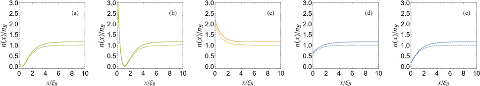
Figure 5: Boson number density profiles for (a) $g_{IB}/(m_{B}\xi_{B})^{-1}=-3$, (b) $-1.5$, (c) $-0.3$, (d) $0.3$, and (e) $1.5$. For all plots $\gamma=0.4$. (a) and (b) are in phase III, (c) is in phase II, and (d) and (e) are in phase I.

We conclude this section by taking a look at the boson number density profile in each phase, with the detailed derivation being left to Appendix A. Figure 5 samples the density profile, $n\left(x\right)$, for a quasi-1D Bose gas along the $x$ dimension. In phase I where $g_{IB}>0$, the ground state is a repulsive polaron $\left(E_{0}>0\right)$ and indeed the impurity (located at the origin $x=0$) repels nearby bosons, creating a hole at its location. As $g_{IB}$ drops from positive to negative, the system enters phase II, where the polaron becomes attractive ($E_{0}<0$) and indeed the impurity pulls nearby bosons towards it, causing bosons to pile up at the impurity location. As $g_{IB}$ is lowered below $g_{c}$, the system enters phase III, where the state becomes a repulsive polaron again $\left(E_{0}>0\right)$, but with a more intriguing density profile. In phase III, in addition to a peak at the impurity location, a hole near (but not exactly at) the impurity location develops. As $g_{IB}$ gets farther away from the critical point $g_{c}$, the peak at $x=0$ continuously decreases while the hole becomes deeper and gets close to the impurity. As such, at the extreme end of phase III, where $g_{IB}=-\infty$, the density profile looks identical to that at the extreme end of phase I where $g_{IB}=+\infty$, demonstrating once again that there is a smooth crossover between the two repulsive phases, as we saw in the polaron energy diagram in Fig. 1.

VI Conclusion

We considered a 1D Bose polaron in the static limit where the Bose gas is described within Bogoliubov theory but the impurity-phonon coupling is modeled by terms that go beyond the Fröhlich paradigm. We diagonalized exactly the beyond-Fröhlich Hamiltonian by applying the generalized Bogoliubov transformation. With our exact solution, we computed boson number density profiles and a polaron energy that is free of divergences common to 1D systems. In Appendix B we use the quasiparticle residue as an example to illustrate that other polaron properties can also be obtained exactly within our approach. Following a detailed stability analysis, we constructed analytically the polaron phase diagram. We found that the repulsive polaron on the negative side of the impurity boson interaction is always thermodynamically unstable due to the presence of a bound state existing slightly above the vacuum dimer energy, whereas the attractive polaron on the negative side of the impurity-boson interaction has a pair of imaginary energies and is therefore always dynamically unstable.

A vast number of problems in many-body physics are too complex to undergo exact treatment. Exactly solvable models, though small in number, are extremely useful. A good grasp of an exactly solvable model helps one to gain insight into, and therefore find ways to solve approximately, more complicated models that can be reduced to the exactly solvable one under limited (but often extreme) conditions. There are many ways in which the present study can benefit research in Bose polarons in cold atoms. Our exact treatment can be adapted straightforwardly to static models in higher dimensions. The ideas behind our exact ansatz can be explored for developing variational ansatzes that approximate, more accurately, the ground states of mobile polarons. The present study provides insight for developing and understanding more realistic models where phonon-phonon interactions are included. When equipped with the local density approximation, our approach can be adapted to treat polarons in traps of sizes much larger than the healing length.

Appendix A Boson number density profiles

The boson number density in position space, $n(\mathbf{r})$, is defined as

$$n\left(\mathbf{r}\right)=\left\langle\hat{\Psi}^{{\dagger}}\left(\mathbf{r}\right)\hat{\Psi}\left(\mathbf{r}\right)\right\rangle,$$ (66)

where $\hat{\Psi}(\mathbf{r})=\sum_{\mathbf{k}}\hat{b}_{\mathbf{k}}^{\prime}e^{i\mathbf{k}\cdot\mathbf{r}}/\sqrt{\mathcal{V}}$ is the boson field operator in position space. After singling out the condensed mode, we express the number density in terms of the noncondensed field modes $\hat{b}_{\mathbf{k}\neq 0}^{\prime}$ as

$$n\left(\mathbf{r}\right) =n_{B}+\sqrt{\frac{n_{B}}{\mathcal{V}}}\sum_{\mathbf{k}}\left(\left\langle\hat{b}_{\mathbf{k}}^{\prime}\right\rangle e^{i\mathbf{k}\cdot\mathbf{r}}+h.c\right)$$

$$\qquad+\frac{1}{\mathcal{V}}\sum_{\mathbf{k},\mathbf{k}^{\prime}}\left\langle\hat{b}_{\mathbf{k}}^{\prime{\dagger}}\hat{b}_{\mathbf{k}^{\prime}}^{\prime}\right\rangle e^{-i\left(\mathbf{k}-\mathbf{k}^{\prime}\right)\cdot\mathbf{r}}.$$ (67)

With the help of Eqs. (3) and (21), we write $\hat{b}_{\mathbf{k}}^{\prime}$ in terms of the shifted phonon field operator $\hat{c}_{\mathbf{k}}$ as

$$\hat{b}_{\mathbf{k}}^{\prime}=\left(u_{\mathbf{k}}z_{\mathbf{k}}-v_{\mathbf{k}}z_{\mathbf{k}}\right)+\left(u_{\mathbf{k}}\hat{c}_{\mathbf{k}}-v_{\mathbf{k}}\hat{c}_{-\mathbf{k}}^{{\dagger}}\right),$$ (68)

where $u_{\mathbf{k}}$ and $v_{\mathbf{k}}$ are defined in Eqs. (4). It then becomes an easy exercise to show that the expectation value of $\hat{b}_{\mathbf{k}}^{\prime}$   and $\hat{b}_{\mathbf{k}}^{\prime{\dagger}}\hat{b}_{\mathbf{k}^{\prime}}^{\prime}$ in Eq. (67) are given, respectively, by

$$\left\langle\hat{b}_{\mathbf{k}}^{\prime}\right\rangle=u_{\mathbf{k}}z_{\mathbf{k}}-v_{\mathbf{k}}z_{\mathbf{k}}$$ (69)

and

$$\left\langle\hat{b}_{\mathbf{k}}^{\prime{\dagger}}\hat{b}_{\mathbf{k}^{\prime}}^{\prime}\right\rangle=\left(u_{\mathbf{k}}z_{\mathbf{k}}-v_{\mathbf{k}}z_{\mathbf{k}}\right)\left(u_{\mathbf{k}^{\prime}}z_{\mathbf{k}^{\prime}}-v_{\mathbf{k}^{\prime}}z_{\mathbf{k}^{\prime}}\right)+\left\langle\cdots\right\rangle,$$ (70)

where

$$\left\langle\cdots\right\rangle =v_{\mathbf{k}}v_{\mathbf{k}^{\prime}}\delta_{\mathbf{k},\mathbf{k}^{\prime}}+u_{\mathbf{k}}u_{\mathbf{k}^{\prime}}\rho_{\mathbf{k}^{\prime}\mathbf{k}}-u_{\mathbf{k}}v_{\mathbf{k}^{\prime}}\kappa_{\mathbf{k},-\mathbf{k}^{\prime}}$$

$$\qquad-v_{\mathbf{k}}u_{\mathbf{k}^{\prime}}\kappa_{\mathbf{k}^{\prime},-\mathbf{k}}+v_{\mathbf{k}}v_{\mathbf{k}^{\prime}}\rho_{-\mathbf{k},-\mathbf{k}^{\prime}},$$ (71)

with

$$\rho_{\mathbf{kk}^{\prime}}=\left\langle\hat{c}_{\mathbf{k}^{\prime}}^{{\dagger}}\hat{c}_{\mathbf{k}}\right\rangle=\sum_{n}V_{n\mathbf{k}}V_{n\mathbf{k}^{\prime}}$$ (72)

the single-particle density matrix element and

$$\kappa_{\mathbf{kk}^{\prime}}=\left\langle\hat{c}_{\mathbf{k}^{\prime}}\hat{c}_{\mathbf{k}}\right\rangle=\sum_{n}V_{n\mathbf{k}}U_{n\mathbf{k}^{\prime}}$$ (73)

the single-particle pair matrix element. Finally, replacing $\langle\hat{b}_{\mathbf{k}}^{\prime}\rangle$ and $\langle\hat{b}_{\mathbf{k}}^{\prime{\dagger}}\hat{b}_{\mathbf{k}^{\prime}}^{\prime}\rangle$ in Eq. (67) with Eqs. (69) and (70), respectively, we arrive at the boson density profile

$$\frac{n\left(\mathbf{r}\right)}{n_{B}} =\frac{n^{M}\left(\mathbf{r}\right)}{n_{B}}+\frac{1}{n_{B}\mathcal{V}}\sum_{\mathbf{k}}v_{\mathbf{k}}^{2}$$

$$+\frac{1}{n_{B}}\sum_{n}\left[I_{uV}^{n}\left(\mathbf{r}\right)^{2}+I_{vV}^{n}\left(\mathbf{r}\right)^{2}-2I_{uV}^{n}\left(\mathbf{r}\right)I_{vU}^{n}\left(\mathbf{r}\right)\right],$$ (74)

where

$$\frac{n^{M}(\mathbf{r})}{n_{B}}=1+\frac{2}{\sqrt{n_{B}}}I\left(\mathbf{r}\right)+\frac{1}{n_{B}}I\left(\mathbf{r}\right)^{2}$$ (75)

is the boson number density profile in the mean-field theory. In the above equations, we introduced four summations:

$$I\left(\mathbf{r}\right) =\frac{1}{\sqrt{\mathcal{V}}}\sum_{\mathbf{k}}z_{\mathbf{k}}\left(u_{\mathbf{k}}-v_{\mathbf{k}}\right)\cos\left(\mathbf{k\cdot r}\right),$$ (76)

$$I_{uV}^{n\text{ }}\left(\mathbf{r}\right) =\frac{1}{\sqrt{\mathcal{V}}}\sum_{\mathbf{k}}u_{\mathbf{k}}V_{n\mathbf{k}}\cos\left(\mathbf{k\cdot r}\right)\text{ ,}$$ (77)

$$I_{vV}^{n}\left(\mathbf{r}\right) =\frac{1}{\sqrt{\mathcal{V}}}\sum_{\mathbf{k}}v_{\mathbf{k}}V_{n\mathbf{k}}\cos\left(\mathbf{k\cdot r}\right),$$ (78)

$$I_{vU}^{n}\left(\mathbf{r}\right) =\frac{1}{\sqrt{\mathcal{V}}}\sum_{\mathbf{k}}v_{\mathbf{k}}U_{n\mathbf{k}}\cos\left(\mathbf{k\cdot r}\right),$$ (79)

which become integrals over momentum in the thermodynamic limit. The density profiles in Fig. 5 are produced using these equations for a 1D Bose gas along the $x$ dimension.

Appendix B Qausiparticle residue

Our exact solution allows observables that are of experimental interest to be evaluated in systems described by the beyond-Fröhlich Hamiltonian. In this Appendix we demonstrate the utility of our exact solution by computing a quantity called the quasiparticle residue, whose definition we review. At zero temperature, phonons are in the phonon vacuum state $\left|0\right\rangle$ in the absence of the impurity, but are in the interacting ground state $\left|\phi\right\rangle$ in the presence of the impurity. The modular square of the overlap integral, $\left\langle 0|\phi\right\rangle$, between the ground phonon state with and without impurity scattering,

$$Z=\left|\left\langle 0|\phi\right\rangle\right|^{2},$$ (80)

is defined as the quasiparticle residue. The quasiparticle residue quantifies the amount of bare impurity (vacuum) that remains in the interacting ground state.

The present problem has a fermionic analog—a localized impurity immersed in a bath of fermionic atoms at zero temperature. In solid-state physics, a well-known example is x-ray absorption, which creates a core hole in the midst of conduction electrons Mahan00Book . Treating the core hole as a localized impurity represented by a static potential, Anderson Anderson (1967) studied the influence of this static potential on a Fermi sea by computing the quasiparticle residue where state $\left|0\right\rangle$ in Eq. (80) is treated as the Fermi sea. The result is summarized in the well-known formula

$$Z=C_{0}N_{F}^{-\left(\delta_{F}/\pi\right)^{2}},$$ (81)

where $N_{F}$ is the total number of fermions and $\delta_{F}=-\tan^{-1}\left(g_{IF}\pi n_{F}\right)$ (with $n_{F}$ the number density) is the phase shift stemming from the $s$-wave scattering of electrons by the impurity with strength $g_{IF}$ and $C_{0}$ is a prefactor which, though complicated, has an analytical expression Ohtaka and Tanabe (1990).

The question we address in this Appendix is what is the analog of Eq. (81) for our system described by the beyond-Fröhlich Hamiltonian? We begin by observing that the state $\left|\phi\right\rangle$ can be obtained from the phonon vacuum $\left|0\right\rangle$ after two successive unitary transformations. The first unitary transformation, $D(z)$, is defined by

$$\hat{c}_{\mathbf{k}} =D(z)\hat{b}_{\mathbf{k}}D^{{\dagger}}(z)$$

$$\hat{c}_{\mathbf{k}}^{{\dagger}} =D(z)\hat{b}_{\mathbf{k}}^{{\dagger}}D^{{\dagger}}(z),$$ (82)

where $D(z)$ is found, with the help of Eqs. (21), to be the well-known displacement operator

$$D(z)=\exp\left[\sum_{\mathbf{k}}\left(\hat{z}_{\mathbf{k}}{b}_{\mathbf{k}}^{{\dagger}}-z_{\mathbf{k}}^{\ast}\hat{b}_{\mathbf{k}}\right)\right].$$ (83)

$D(z)$ transforms $\hat{H}$, the Hamiltonian in Eq. (8), to

$$\hat{H}^{\prime}=D^{{\dagger}}(z)\hat{H}D(z),$$ (84)

where $\hat{H}^{\prime}$ is identical to $\hat{H}$ in Eq. (22) except $\hat{c}_{\mathbf{k}}$ ($\hat{c}_{\mathbf{k}}^{{\dagger}}$) in Eq. (22) is replaced with $\hat{b}_{\mathbf{k}}$ ($\hat{b}_{\mathbf{k}}^{{\dagger}}$) which are now interpreted as the field operators in the Hilbert space defined by $D(z)$.

The second unitary transformation, $S$, is defined by

$$\hat{d}_{n} =S\hat{b}_{\mathbf{k}_{n}}S^{{\dagger}}$$ (85)

$$\hat{d}_{n}^{{\dagger}} =S\hat{b}_{\mathbf{k}_{n}}^{{\dagger}}S^{{\dagger}},$$ (86)

which can be solved, in principle, from the Bogoliubov transformation (23) [but with $\hat{c}_{\mathbf{k}}$ ($\hat{c}_{\mathbf{k}}^{{\dagger}}$) replaced with $\hat{b}_{\mathbf{k}}$ ($\hat{b}_{\mathbf{k}}^{{\dagger}}$)] in terms of operators defined in Fock space. $S$ transforms $\hat{H}^{\prime}$ in Eq. (84) to

$$\hat{H}^{\prime\prime}=S^{{\dagger}}\hat{H}^{\prime}S,$$ (87)

where $\hat{H}^{\prime\prime}$ is identical to $\hat{H}$ in Eq. (28) except $\hat{d}_{n}$ ($\hat{d}_{n}^{{\dagger}}$) in Eq. (28) are replaced with $\hat{b}_{\mathbf{k}_{n}}$ ($\hat{b}_{\mathbf{k}_{n}}^{{\dagger}}$) which are now interpreted as field operators in the Hilbert space defined by $S$.

As a result, the interacting polaron state is given by

$$|\phi\rangle=D(z)S|0\rangle,$$ (88)

where $S|0\rangle$ is a normalized state given by blaizot96QuantumTheoryBook

$$S\left|0\right\rangle=\frac{\exp\left(\frac{1}{2}\sum_{\mathbf{k},\mathbf{k}^{\prime}}\hat{b}_{\mathbf{k}}^{{\dagger}}W_{\mathbf{kk}^{\prime}}\hat{b}_{\mathbf{k}^{\prime}}^{{\dagger}}\right)}{\sqrt[4]{\det\left(U^{{\dagger}}U\right)}}\left|0\right\rangle,$$ (89)

where $W$ is a matrix defined as

$$W=U^{\ast-1}V^{\ast}.$$ (90)

The quasiparticle residue $Z$ in Eq. (80) becomes the overlap between coherent state $\left|-z\right\rangle$ and state $S\left|0\right\rangle$: $Z=\left|\left\langle-z\right|S\left|0\right\rangle\right|^{2}$ or explicitly

$$Z=\frac{\exp\left[\sum_{\mathbf{k}}\left(\sum_{\mathbf{k}^{\prime}}z_{\mathbf{k}}W_{\mathbf{kk}^{\prime}}z_{\mathbf{k}^{\prime}}-z_{\mathbf{k}}^{2}\right)\right]}{\left|\det U\right|},$$ (91)

where the use of $\langle-z|0\rangle=\exp(-\sum z_{\mathbf{k}}^{2}/2)$ is made and all variables involved are assumed to be real. Equation (91) is the analog of Eq. (81) we sought for our model. As expected, Eq. (91) simplifies to the mean-field result $Z=\exp\left(-\sum_{\mathbf{k}}z_{\mathbf{k}}^{2}\right)$ Shashi et al. (2014); Grusdt et al. (2017b), in the absence of quantum fluctuations where $V$ is a null matrix and $U$ is an identity matrix

References

- (1) L. D. Landau, Phys. Z. Sowjetunion 3, 664 (1933); L. D. Landau and S. I. Pekar, Zh. Eksp. Teor. Fiz. 18, 419 (1948).
- (2) S. I. Pekar, Zh. Eksp. Teor. Fiz. 16, 341 (1946).
- Fröhlich (1954) H. Fröhlich, Adv. Phys. 3, 325 (1954).
- (4) A. S. Alexandrov, Polarons in Advanced Materials (Springer-Verlag, Berlin, 2007).
- Lee et al. (1953) T. D. Lee, F. E. Low, and D. Pines, Phys. Rev. 90, 297 (1953).
- Feynman (1955) R. P. Feynman, Phys. Rev. 97, 660 (1955).
- Chin et al. (2010) C. Chin, R. Grimm, P. Julienne, and E. Tiesinga, Rev. Mod. Phys. 82, 1225 (2010).
- Devreese (2013) J. T. Devreese, arXiv:1012.4576 (2013).
- Grusdt and Demler (2015) F. Grusdt and E. Demler, arXiv:1510.04934 (2015).
- Astrakharchik and Pitaevskii (2004) G. E. Astrakharchik and L. P. Pitaevskii, Phys. Rev. A 70, 013608 (2004).
- Cucchietti and Timmermans (2006) F. M. Cucchietti and E. Timmermans, Phys. Rev. Lett. 96, 210401 (2006).
- Kalas and Blume (2006) R. M. Kalas and D. Blume, Phys. Rev. A 73, 043608 (2006).
- Bruderer et al. (2008) M. Bruderer, A. Klein, S. R. Clark, and D. Jaksch, New Journal of Physics 10, 033015 (2008).
- Huang and Wan (2009) B.-B. Huang and S.-L. Wan, Chinese Physics Letters 26, 080302 (2009).
- Tempere et al. (2009) J. Tempere, W. Casteels, M. K. Oberthaler, S. Knoop, E. Timmermans, and J. T. Devreese, Phys. Rev. B 80, 184504 (2009).
- Casteels et al. (2011) W. Casteels, T. Cauteren, J. Tempere, and J. T. Devreese, Laser Physics 21, 1480 (2011).
- Casteels et al. (2012) W. Casteels, J. Tempere, and J. T. Devreese, Phys. Rev. A 86, 043614 (2012).
- Rath and Schmidt (2013) S. P. Rath and R. Schmidt, Phys. Rev. A 88, 053632 (2013).
- Kain and Ling (2014) B. Kain and H. Y. Ling, Phys. Rev. A 89, 023612 (2014).
- Shashi et al. (2014) A. Shashi, F. Grusdt, D. A. Abanin, and E. Demler, Phys. Rev. A 89, 053617 (2014).
- Li and Das Sarma (2014) W. Li and S. Das Sarma, Phys. Rev. A 90, 013618 (2014).
- (22) F. Grusdt, Y. E. Shchadilova, A. N. Rubtsov, and E. Demler, Scientific Reports 5, 12124 (2015).
- Ardila and Giorgini (2015) L. A. Peña Ardila and S. Giorgini, Phys. Rev. A 92, 033612 (2015).
- Vlietinck et al. (2015) J. Vlietinck, W. Casteels, K. V. Houcke, J. Tempere, J. Ryckebusch, and J. T. Devreese, New Journal of Physics 17, 033023 (2015).
- Shchadilova et al. (2016a) Y. E. Shchadilova, F. Grusdt, A. N. Rubtsov, and E. Demler, Phys. Rev. A 93, 043606 (2016a).
- Christensen et al. (2015) R. S. Christensen, J. Levinsen, and G. M. Bruun, Phys. Rev. Lett. 115, 160401 (2015).
- Ardila and Giorgini (2016) L. A. Peña Ardila and S. Giorgini, Phys. Rev. A 94, 063640 (2016).
- Levinsen et al. (2015) J. Levinsen, M. M. Parish, and G. M. Bruun, Phys. Rev. Lett. 115, 125302 (2015).
- Kain and Ling (2016) B. Kain and H. Y. Ling, Phys. Rev. A 94, 013621 (2016).
- Dehkharghani et al. (2015) A. S. Dehkharghani, A. G. Volosniev, and N. T. Zinner, Phys. Rev. A 92, 031601 (2015).
- Schmidt et al. (2016) R. Schmidt, H. R. Sadeghpour, and E. Demler, Phys. Rev. Lett. 116, 105302 (2016).
- Parisi and Giorgini (2017) L. Parisi and S. Giorgini, Phys. Rev. A 95, 023619 (2017).
- Sun et al. (2017) M. Sun, H. Zhai, and X. Cui, Phys. Rev. Lett. 119, 013401 (2017).
- Volosniev and Hammer (2017) A. G. Volosniev and H.-W. Hammer, Phys. Rev. A 96, 031601 (2017).
- Yoshida et al. (2018) S. M. Yoshida, S. Endo, J. Levinsen, and M. M. Parish, Phys. Rev. X 8, 011024 (2018).
- (36) S. M. Yoshida, Z.-Y. Shi, J. Levinsen, and M. M. Parish, arXiv:1807.09992.
- (37) Z.-Y. Shi, S. M. Yoshida, M. M. Parish, and J. Levinsen, arXiv:1807.09948.
- Catani et al. (2012) J. Catani, G. Lamporesi, D. Naik, M. Gring, M. Inguscio, F. Minardi, A. Kantian, and T. Giamarchi, Phys. Rev. A 85, 023623 (2012).
- Hu et al. (2016) M.-G. Hu, M. J. Van de Graaff, D. Kedar, J. P. Corson, E. A. Cornell, and D. S. Jin, Phys. Rev. Lett. 117, 055301 (2016).
- Jørgensen et al. (2016) N. B. Jørgensen, L. Wacker, K. T. Skalmstang, M. M. Parish, J. Levinsen, R. S. Christensen, G. M. Bruun, and J. J. Arlt, Phys. Rev. Lett. 117, 055302 (2016).
- Meinert et al. (2017) F. Meinert, M. Knap, E. Kirilov, K. Jag-Lauber, M. B. Zvonarev, E. Demler, and H.-C. Nägerl, Science 356, 945 (2017).
- (42) R. P. Feynman, Statistical Mechanics (Addison-Wesley, Reading, MA, 1990).
- Shchadilova et al. (2016b) Y. E. Shchadilova, R. Schmidt, F. Grusdt, and E. Demler, Phys. Rev. Lett. 117, 113002 (2016b).
- Grusdt et al. (2017a) F. Grusdt, R. Schmidt, Y. E. Shchadilova, and E. Demler, Phys. Rev. A 96, 013607 (2017a).
- Grusdt et al. (2017b) F. Grusdt, G. E. Astrakharchik, and E. Demler, New Journal of Physics 19, 103035 (2017b).
- Knap et al. (2012) M. Knap, A. Shashi, Y. Nishida, A. Imambekov, D. A. Abanin, and E. Demler, Phys. Rev. X 2, 041020 (2012).
- Olshanii (1998) M. Olshanii, Phys. Rev. Lett. 81, 938 (1998).
- Bergeman et al. (2003) T. Bergeman, M. G. Moore, and M. Olshanii, Phys. Rev. Lett. 91, 163201 (2003).
- Peano et al. (2005) V. Peano, M. Thorwart, C. Mora, and R. Egger, New Journal of Physics 7, 192 (2005).
- Hohenberg (1967) P. C. Hohenberg, Phys. Rev. 158, 383 (1967).
- Mermin and Wagner (1966) N. D. Mermin and H. Wagner, Phys. Rev. Lett. 17, 1133 (1966).
- Petrov et al. (2000) D. S. Petrov, G. V. Shlyapnikov, and J. T. M. Walraven, Phys. Rev. Lett. 85, 3745 (2000).
- Lieb and Liniger (1963) E. H. Lieb and W. Liniger, Phys. Rev. 130, 1605 (1963).
- Lieb (1963) E. H. Lieb, Phys. Rev. 130, 1616 (1963).
- (55) G. D. Mahan, Many-Particle Physics, 3rd ed. (Kluwer Academic/Plenum, New York, 2000).
- (56) D. F. Walls and G. J. Milburn, Quantum Optics (Springer-Verlag, Berlin, 2008).
- Hasan and Kane (2010) M. Z. Hasan and C. L. Kane, Rev. Mod. Phys. 82, 3045 (2010).
- Kain and Ling (2017) B. Kain and H. Y. Ling, Phys. Rev. A 96, 033627 (2017).
- Anderson (1967) P. W. Anderson, Phys. Rev. Lett. 18, 1049 (1967).
- Ohtaka and Tanabe (1990) K. Ohtaka and Y. Tanabe, Rev. Mod. Phys. 62, 929 (1990).
- (61) J.-P. Blaizot and G. Ripka, “Quantum Theory of Finite Systems,” The MIT Press, Cambridge, Massachusetts (1986).