Novel Multi-Agent Models for Chemical Self-assembly

Abstract

The chemical self-assembly has been considered as one of most important scientific problems in the 21th Century; however, since the process of self-assembly is very complex, there is few mathematic theory for it currently. This paper provides a novel multi-agent model for chemical self-assembly, where the interaction between agents adopts the classic Lennard-Jones potential. Under this model, we propose an optimal problem by taking the temperature as the control input, and choosing the internal energy as the optimal object. A numerical solution for our optimal problem is also developed. Simulations show that our control scheme can improve the product of self-assembly. Further more, we give a strict analysis for the self-assembly model without noise, which corresponds to an attraction-repulsion multi-agent system, and prove it converges to a stable configuration eventually.

, , ,

1 Introduction

Self-assembly is the process in which disordered components form an organized structure with local interactions among the components without external forces (Whitesides and Grzybowski, 2002). It reveals how disordered components form the ordered structure in nature and the understanding of self-assembly could help us create nano-structured materials and build new nanostructures. This topic has raised a lot of interest in physics, chemistry and biology in recent several decades. In the Science 125th anniversary, the magazine raised 125 important scientific problems in 21st century (Service, 2005). Among these problems, they picked 25 most important ones, one of which is “How Far Can We Push Chemical Self-Assembly?”

Recent developments of self-assembly in chemistry have been made in both experiments (Nykypanchuk et al., 2008) and computational simulations (Wilber et al., 2009). Experimental scientists have carried on a large number of self-assembly experiments, including molecular, nanoparticles and protein molecular. A lot of assembly products have been discovered. Theoretical scientists use computers to simulate the self-assembly process(Klotsa and Jack, 2013). However, since there are too many kinds of assembly products, and the assembly process is very complex, the hidden laws of self-assembly are hard to find through experiments and simulations. Currently, there is few mathematic theory for the self-assembly. This paper tries to model the self-assembly by multi-agent systems and build an optimal control on them.

Multi-agent systems composed by multiple interacting agents have drawn considerable attention from various fields in the past two decades. In physics, the synchronization phenomena of coupled oscillators, flashing fireflies, and chirping crickets is investigated (Kuramoto, 1975; Acebrón et al., 2005); in biology, scientists model animal flocking behavior (Buhl et al., 2006; Vicsek et al., 1995); in sociology, the emergence and spread of public opinions can also be investigated as multi-agent system(Deffuant et al., 2000; Hegselmann et al., 2002). A central issue of multi-agent system study is to understand how local interactions among the elements lead to collective behavior of the whole group. Because of the importance, effort has been devoted to the mathematical analysis of collective behavior of multi-agent systems (Chen et al., 2017). A new method called as “soft control” has been proposed which keeps the local rule of the existing agents in the system and controls the collective behavior indirectly by changing exterior environment (Han et al., 2006).

In this paper, we model the dynamics of self-assembly as a multi-agent system, in which each agent denotes a component, and the interaction between agents denotes the force between components. Because the real self-assembly is very complex, we need make some simplification. In our model, we assume the agents are homogeneous and isotropic, and the interaction between agents adopts the classical Lennard-Jones potential. Such a system corresponds to some practical systems such as the self-assembly of gold nanoparticles(Gittins et al., 2002). Because the temperature is crucial in self-assembly, we treat it as a control input, and try to find its optimal control to the assembly product we want. This control method can also be considered as a soft control, however different from the method of adding some special agents in previous work (Han et al., 2006).

The contribution of this paper can be formulated as follows: First, in this paper we propose a new mathematical model for chemical self-assembly. As mentioned above, the mathematical models and analysis are very important to understand the behind law of chemical self-assembly, however they are very few currently. Our model provides an enter point for the analysis of self-assembly. Although our model is ideal, it still keeps the essential feature of chemical self-assembly. Also, it is possible that we could extend the model to some real assembly experiments like the self-assembly of gold nanoparticles (Kaplan, 2006).

Secondly, we put forward a mathematical method to find the optimal temperature control for our model. It is well-known that the temperature is a critical value in chemical systems. How to find the optimal temperature control is an important issue in the research of chemical self-assembly. Currently chemists mainly adopt empirical methods, and still lack the guidance of mathematical theory. Our method is a way to get the optimal control for our model, and hope it can be extended to some real chemical systems.

Finally, we give a strict analysis for the multi-agent self-assembly model without noise, and prove it will converge to a stable configuration eventually. The noise-free self-assembly model can be treated as a multi-agent attractive-repulsive model, which has attracted a lot of interest in the study of flocking algorithms. Our system and results can provide some new idea for the modeling and analysis to the flocking research.

The rest of this article is organized as follows: In Section 2 we introduce a multi-agent model for chemical self-assembly and give a result for the noise-free case. In Section 3 we propose an optimal control problem to our model and explore a numerical solution. Section 4 provide some simulations using our control laws, while Section 5 concludes this paper.

2 A multi-agent model for self-assembly

This section proposes a novel multi-agent model for the chemical self-assembly. The model considers $N$ homogeneous and isotropic particles move in a fluid, and each particle $i$ contains a position variable $X_{i}=X_{i}(t)\in\mathbb{R}^{3}$ and a velocity variable $V_{i}=V_{i}(t)\in\mathbb{R}^{3}$. We use the classic Langevin equation to formulate the dynamics of the particles, which is, for $t\geq 0$ and $1\leq i\leq N$, the position and velocity of particle $i$ is driven by

$$\left\{\begin{array}[]{l}\dot{X}_{i}=V_{i}\\ \dot{V}_{i}=-BV_{i}+f_{i}+\xi_{i}\end{array}\right.,$$ (3)

where $B$ is a constant denoting the damping coefficient of each particle in the fluid, $f_{i}=f_{i}(t)$ is the force of particle $i$ affected by other particles, and $\xi_{i}=\xi_{i}(t)$ denotes the Brownian force produced by the thermal noise.

In practical chemical self-assembly, the interaction between particles is very complex (e.g. Van der Waals, capillary, $\pi-\pi$ hydrogen bonds). To be simplified, this paper assumes the interaction between particles is additive, and can be described by the classic Lennard-Jones (L-J) potential. In mathematics, the L-J potential between two particles $i$ and $j$ can be formulated as

$$\Phi_{ij}=\Phi_{ij}(t)=\varepsilon\Big{(}\frac{r_{m}}{r_{ij}}\Big{)}^{12}-2\varepsilon\Big{(}\frac{r_{m}}{r_{ij}}\Big{)}^{6},$$ (4)

where $\varepsilon$ and $r_{m}$ are constants denoting the depth of the potential well and the distance at which the potential reaches its minimum respectively, and

$$r_{ij}=r_{ij}(t)=\|X_{i}-X_{j}\|_{2}$$

denotes the distance between the particle $i$ and $j$ at time $t$. Here $\|\cdot\|_{2}$ denotes the Euclidean norm. Thus, the force of particle $i$ affected by particle $j$ is

$$\begin{aligned} f_{ij}=f_{ij}(t)=-\nabla\Phi_{ij}&=12\varepsilon\left(\frac{r_{m}^{6}}{r_{ij}^{7}}-\frac{r_{m}^{12}}{r_{ij}^{13}}\right)\left(-\nabla r_{ij}\right)\\ &=12\varepsilon\left(\frac{r_{m}^{6}}{r_{ij}^{8}}-\frac{r_{m}^{12}}{r_{ij}^{14}}\right)\left(X_{j}-X_{i}\right),\end{aligned}$$

where $\nabla g$ denotes the gradient of function $g$ in $\mathbb{R}^{3}$ (i.e., $\nabla g=(\frac{\partial g}{\partial x},\frac{\partial g}{\partial y},\frac{\partial g}{\partial z})$). Consider the forces between particles are additive, so the total force of particle $i$ affected by other particles is

$$\begin{aligned} f_{i}&=f_{i}(t)=\sum_{j\neq i}f_{ij}\\ &=\sum_{j\neq i}12\varepsilon\left(\frac{r_{m}^{6}}{r_{ij}^{8}}-\frac{r_{m}^{12}}{r_{ij}^{14}}\right)\left(X_{j}-X_{i}\right).\end{aligned}$$ (5)

According to the Langevin equation theory (Coffey and Kalmykov, 2004), the Brownian force $\xi_{i}$ has zero mean and its covariance is

$$\mbox{Cov}(\xi_{i}(t),\xi_{j}(t^{\prime}))=\left\{\begin{array}[]{ll}0,&\mbox{if~{}}i\neq j\\ 2Bk_{b}U\delta(t-t^{\prime}),&\mbox{otherwise}\end{array}\right.,$$

where $k_{b}$ denotes the Boltzmann constant, $U$ denotes the absolute temperature, and $\delta(t)$ denotes the Dirac delta function.

The system (3) seems ideal, however it keeps the essential feature of chemical self-assembly. Also, it is possible to extend this model to some real assembly systems like the self-assembly of gold nanoparticles.

For the convenience of mathematical analysis, the system (3) can be transformed to a group of stochastic differential equations. By the Langevin equation theory (Coffey and Kalmykov, 2004), the integration of the force $\xi_{i}$, $\int_{0}^{t}\xi_{i}(\tau)\mathrm{d}\tau$, has the same property as $\sqrt{2Bk_{b}U}W_{i}(t)$, where $W_{i}(t)$ is a standard Wiener process independent with $\{W_{j}(t)\}_{j\neq i}$. Therefore, $\xi_{i}(t)\mathrm{d}t=\mathrm{d}[\int_{0}^{t}\xi_{i}(\tau)\mathrm{d}\tau]$ can be written as $\sqrt{2Bk_{b}U}\mathrm{d}W_{i}(t)$. and the system (3) can be written as the following stochastic differential equations:

$$\left\{\begin{array}[]{l}\mathrm{d}{X}_{i}={V}_{i}\mathrm{d}t\\ \mathrm{d}{V}_{i}=(-BV_{i}+f_{i})\mathrm{d}t+\sqrt{2Bk_{b}U}\mathrm{d}W_{i}(t)\end{array}\right..$$ (9)

3 Optimal control for self-assembly model

The Hamiltonian plays a key role in a physical system. In this paper our prime goal is to minimize the Hamiltonian, which indicates the assembly product reaches a most stable state. By (4), the Hamiltonian of our system (3) is

$$H=H(t)=\frac{1}{2}\sum_{i=1}^{N}V_{i}^{T}V_{i}+\sum_{i<j}\varepsilon\left(\frac{r_{m}^{12}}{r_{ij}^{12}}-2\frac{r_{m}^{6}}{r_{ij}^{6}}\right).$$ (10)

We also need to choose a suitable control input. In real chemical self-assembly, the particles are very small, and are hard to be controlled directed; however we can control the external environment to intervene the assembly product. Temperature control is very important in chemical self-assembly. At present, it is mainly based on empirical method and lacks mathematical theory guidance. In this paper, we try to build a method on how to control the temperature to minimize the Hamiltonian. This method can be also treated as a soft control which initially proposed by (Han et al., 2006).

To be simplified we set $u(t):=k_{b}U(t)$ as the control input, and rewrite the system (9) as the following dynamics:

$$\left\{\begin{array}[]{l}\mathrm{d}{X}_{i}={V}_{i}\mathrm{dt}\\ \mathrm{d}{V}_{i}=(-BV_{i}+f_{i})\mathrm{d}t+\sqrt{2Bu}\mathrm{d}W_{i}(t)\end{array}\right..$$ (13)

We aim to minimize the Hamiltonian $H(T)$ with $T$ being a fixed time. According to (10) and (9), $H(t)$ is a stochastic process and we calculate the differential of $H(t)$.

$$\begin{aligned} \mathrm{d}H=&\frac{1}{2}\sum_{i=1}^{N}\mathrm{d}(V_{i}^{T}V_{i})+\frac{1}{2}\varepsilon\sum_{i\neq j}\mathrm{d}\left(\frac{r_{m}^{12}}{r_{ij}^{12}}-2\frac{r_{m}^{6}}{r_{ij}^{6}}\right).\end{aligned}$$ (14)

The first part $\frac{1}{2}\sum_{i=1}^{N}\mathrm{d}(V_{i}^{T}V_{i})$ involves $V_{i}(t)$, we must use Itô’s formula to calculate its differential. According to the general Itô’s formula (Theorem 4.2.1 in (Øksendal, 1985)),

$$\begin{aligned} &\frac{1}{2}\sum_{i=1}^{N}\mathrm{d}(V_{i}^{T}V_{i})\\ &=\frac{1}{2}\sum_{i=1}^{N}(2V_{i}^{T}\mathrm{d}V_{i}+\mathrm{d}V_{i}^{T}\mathrm{d}V_{i})\\ &=\frac{1}{2}\sum_{i=1}^{N}\left[2\left(-BV_{i}+f_{i}\right)^{T}V_{i}\mathrm{d}t+2\sqrt{2Bu}V_{i}\mathrm{d}W_{i}(t)\right]\\ &~{}~{}+\frac{1}{2}\sum_{i=1}^{N}\mathrm{d}V_{i}^{T}\mathrm{d}V_{i}\\ &=\sum_{i=1}^{N}(-BV_{i}^{T}V_{i})\mathrm{d}t+f_{i}^{T}V_{i}\mathrm{d}t+\sqrt{2Bu}V_{i}\mathrm{d}W_{i}(t)\\ &~{}~{}+\frac{1}{2}\mathrm{d}V_{i}^{T}\mathrm{d}V_{i}.\end{aligned}$$ (15)

According to the stochastic differential equation theory, we have $\mathrm{d}t\cdot\mathrm{d}t=\mathrm{d}t\cdot\mathrm{d}W(t)=\mathrm{d}W(t)\cdot\mathrm{d}t=0$, and $\mathrm{d}W(t)\cdot\mathrm{d}W(t)=\mathrm{d}t$. Then, $\mathrm{d}V_{i}^{T}\mathrm{d}V_{i}$ can be expanded into follows:

$$\begin{aligned} &\mathrm{d}V_{i}^{T}\mathrm{d}V_{i}\\ &=\left[\left(-BV_{i}^{T}+f_{i}^{T}\right)\mathrm{d}t+\sqrt{2Bu}\mathrm{d}W_{i}(t)\right]^{T}\\ &~{}~{}~{}~{}\times\left[\left(-BV_{i}^{T}+f_{i}^{T}\right)\mathrm{d}t+\sqrt{2Bu}\mathrm{d}W_{i}(t)\right]\\ &=2Bu\mathrm{d}W_{i}(t)\mathrm{d}W_{i}(t)\\ &=2Bu\mathrm{d}t.\end{aligned}$$ (16)

The second part in (14) only involves $X_{i}(t)$, Itô’s formula is not needed.

$$\begin{aligned} &\frac{1}{2}\varepsilon\sum_{i\neq j}\mathrm{d}\left(\frac{r_{m}^{12}}{r_{ij}^{12}}-2\frac{r_{m}^{6}}{r_{ij}^{6}}\right)=6\sum_{i\neq j}\varepsilon\left(\frac{r_{m}^{6}}{r_{ij}^{7}}-\frac{r_{m}^{12}}{r_{ij}^{13}}\right)\mathrm{d}r_{ij}\\ &=6\sum_{i\neq j}\varepsilon\left(\frac{r_{m}^{6}}{r_{ij}^{7}}-\frac{r_{m}^{12}}{r_{ij}^{13}}\right)\frac{1}{r_{ij}}\left(X_{i}-X{j}\right)^{T}\left(V_{i}-V_{j}\right)\mathrm{d}t\\ &=6\sum_{i\neq j}\varepsilon\left(\frac{r_{m}^{6}}{r_{ij}^{8}}-\frac{r_{m}^{12}}{r_{ij}^{14}}\right)\\ &~{}~{}~{}~{}\times\left[\left(X_{i}-X{j}\right)^{T}V_{i}+\left(X_{j}-X{i}\right)^{T}V_{j}\right]\mathrm{d}t\\ &=\left[\frac{1}{2}\sum_{i=1}^{N}\left(-f_{i}^{T}V_{i}\right)+\frac{1}{2}\sum_{j=1}^{N}\left(-f_{j}V_{j}\right)\right]\mathrm{d}t\\ &=\sum_{i=1}^{N}-f_{i}^{T}V_{i}\mathrm{d}t.\end{aligned}$$ (17)

By (15), (16) and (17), the differential of $H(t)$ is

$$\begin{aligned} \mathrm{d}H=&\sum_{i=1}^{N}(-BV_{i}^{T}V_{i}+Bu)\mathrm{d}t+\sqrt{2Bu}V_{i}\mathrm{d}W_{i}(t).\end{aligned}$$ (18)

The Hamiltonian at time $T$ could be represented as follows:

$$\begin{aligned} H(T)=&H(0)+\int_{0}^{T}\mathrm{d}H\\ =&H(0)+\int_{0}^{T}\sum_{i=1}^{N}(-BV_{i}^{T}V_{i}+Bu)\mathrm{d}t\\ &+\int_{0}^{T}\sum_{i=1}^{N}\sqrt{2Bu}V_{i}\mathrm{d}W_{i}(t).\end{aligned}$$ (19)

Because the Hamiltonian $H$ is stochastic, we use $E[H(T)]$ as the optimization object. Because the expectation of Itô’s integral is zero, from (19) we have

$$\mathrm{E}H(T)=\mathrm{E}H(0)+\int_{0}^{T}B\sum_{i=1}^{N}(-EV_{i}^{T}V_{i}+u)\mathrm{d}t.$$ (20)

Our aim is to find the optimal control $u(t)$ to minimize the value of $\mathrm{E}H(T)$.

Because the temperature is limited by an allowable region in a chemical experiment, we assume the lower and upper bounds of $u$ are $u_{\min}$ and $u_{\max}$ respectively. Then, we consider the following optimization problem:

$$\begin{aligned} \min~{}&\mathrm{E}H(0)+\int_{0}^{T}B\sum_{i=1}^{N}(-EV_{i}^{T}V_{i}+u)\mathrm{d}t\\ s.t.&\ u_{\min}\leq u\leq u_{\max},\\ &\mathrm{d}{V}_{i}=(-BV_{i}+f_{i})\mathrm{d}t+\sqrt{2Bu}\mathrm{d}W_{i}(t),i=1,...,N.\end{aligned}$$ (21)

By (20) the optimization objective $\mathrm{E}H(T)$ is a nonlinear function, and by (13) the velocity $V_{i}(t)$ is a very complex stochastic process which depends on not only the control input $u(t)$, but also the states of other particles. It is hard to get the analytic optimal solution. As an alternative, we will develop a numerical method to optimize $\mathrm{E}H(T)$.

3.1 Numerical method for the optimal control problem (21)

Firstly we use Monte Carlo method to transform the stochastic constraints in (21) into deterministic constraints. Set $X(t):=(X_{1}(t),\ldots,X_{N}(t))$, $V(t):=(V_{1}(t),\ldots,V_{N}(t))$, and $W(t):=(W_{1}(t),\ldots,W_{N}(t))$. Let $W(0:T)$ denote the trajectory $W(t),0\leq t\leq T$. We randomly select $M$ sample trajectories $\{X^{k}(0),V^{k}(0),W^{k}(0:T)\}_{1\leq k\leq M}$ from the sample space of $\{X(0),V(0),W(0:T)\}$, and change the stochastic constraints in (21) into the following constraints:

$$\begin{aligned} \mathrm{d}{V}_{i}^{k}&=(-BV_{i}^{k}+f_{i})\mathrm{d}t+\sqrt{2Bu}\mathrm{d}W_{i}^{k},\\ &~{}\forall 1\leq i\leq N,1\leq k\leq M,\end{aligned}$$ (22)

where $V_{i}^{k}$ and $W_{i}^{k}$ denote the $i$-th element of $V^{k}$ and $W^{k}$ corresponding to particle $i$.

If $M$ is large enough, the objective function in (21) can be approximated by

$$\begin{aligned} &\mathrm{E}H(0)+\int_{0}^{T}B\sum_{i=1}^{N}(-EV_{i}^{T}V_{i}+u)\mathrm{d}t\\ &\approx\frac{1}{M}\sum_{k=1}^{M}\Big{[}H(0)+B\int_{0}^{T}\sum_{i=1}^{N}(-(V_{i}^{k})^{T}V_{i}^{k}+u)\mathrm{d}t\Big{]}.\end{aligned}$$ (23)

Secondly, we discretize the time interval $[0,T]$ into $N_{T}+1$ points $0,\Delta t,\ldots N_{T}\Delta t$ with $\Delta t:=\frac{T}{N_{T}}$. Let $t_{n}:=n\Delta t$. Then, we use ($V_{i}^{k}(0),V_{i}^{k}(\Delta t),\ldots,V_{i}^{k}(N_{T}\Delta t)$) to approximate the trajectory of $V_{i}^{k}(0:T)$, and $(u(0),u(\Delta t),...,u(N_{T}\Delta t))$ to approximate the continuous-time control $u(0:T)$. Notice that

$$X_{i}(t)=\int_{0}^{t}V_{i}(s)\mathrm{d}s+X_{i}(0),$$

so at time $t_{n}$, the position of each particle $i$ can be approximated by

$$X_{i}(t_{n})\approx\Delta t\sum_{q=1}^{n}V_{i}(t_{q})+X_{i}(0).$$ (24)

By (5) and (24), the force $f_{i}(t_{n})$ can also be approximated by

$$f_{i}(t_{n})\approx f_{i}\Big{(}\Delta t\sum_{q=1}^{n}V_{1}(t_{q}),\ldots,\Delta t\sum_{q=1}^{n}V_{N}(t_{q})\Big{)}.$$ (25)

Corresponding, the differential $dW_{i}^{k}(t_{n})$ is approximated by the difference $W^{k}_{i}(t_{n})-W^{k}_{i}(t_{n-1})$, where the difference are independent random variables which have normal distribution and its variance is $\Delta t$ (Glasserman, 2004). From this and (25), the differential equation (22) can be approximated by the following difference equation:

$$\begin{aligned} &V_{i}^{k}(t_{n+1})-V_{i}^{k}(t_{n})\approx-BV_{i}^{k}(t_{n+1})\Delta t\\ &+f_{i}(\Delta t\sum_{q=1}^{n}V_{1}^{k}(t_{q}),\ldots,\Delta t\sum_{q=1}^{n}V^{k}_{N}(t_{q}))\Delta t\\ &+\sqrt{2Bu(t_{n+}1)}(W^{k}_{i}(t_{n+1})-W^{k}_{i}(t_{n})),\\ &\ \ i=1,\ldots,N,k=1,\ldots,M,n=0,\ldots,N_{T}-1.\end{aligned}$$ (26)

Similarly, we discretize the right side of (23) and get

$$\begin{aligned} &\mathrm{E}H(0)+\int_{0}^{T}B\sum_{i=1}^{N}(-EV_{i}^{T}V_{i}+u)\mathrm{d}t\\ &\approx\frac{1}{M}\sum_{k=1}^{M}\big{[}\mathrm{E}H(0)-B\Delta t\sum_{n=1}^{N_{T}}\sum_{i=1}^{N}V_{i}^{k}(t_{n})^{T}V_{i}^{k}(t_{n})\\ &~{}~{}~{}~{}+NB\Delta t\sum_{n=1}^{N_{T}}u(t_{n})\big{]}.\end{aligned}$$ (27)

By (27) and (26), the optimal control problem (21) can be approximated by the follows:

$$\begin{aligned} \min&~{}\frac{1}{M}\sum_{k=1}^{M}\big{[}\mathrm{E}H(0)-B\Delta t\sum_{n=1}^{N_{T}}\sum_{i=1}^{N}V_{i}^{k}(t_{n})^{T}V_{i}^{k}(t_{n})\\ &+NB\Delta t\sum_{n=1}^{N_{T}}u(t_{n})\big{]}.\\ s.t.&\ u_{\min}\leq u(t_{n})\leq u_{\max},\\ &V_{i}^{k}(t_{n+1})-V_{i}^{k}(t_{n})=-BV_{i}^{k}(t_{n+1})\Delta t\\ &+f_{i}(\Delta t\sum_{q=1}^{n}V_{1}^{k}(t_{q}),\ldots,\Delta t\sum_{q=1}^{n}V^{k}_{N}(t_{q}))\Delta t\\ &+\sqrt{2Bu(t_{n+1})}(W^{k}_{i}(t_{n+1})-W^{k}_{i}(t_{n})),\\ &\ \ i=1,\ldots,N,k=1,\ldots,M,n=0,\ldots,N_{T}-1.\end{aligned}$$ (28)

We can solve (28) by sequential quadratic programming (SQP) method which is suitable for non-linear optimization with constraints (Spellucci, 1998).

3.2 A numerical solution and comparison with natural cooling

In this section, we provide a numerical example to solve the problem (28). Choose the particle number $N=30$, the stop time $T=10$, and the time step $\Delta t=0.1$. Set $\varepsilon$ and $r_{m}$ in (5) to be 3 and 2 respectively. Let the damping coefficient $B=2$. The initial position $X_{i}(0)(1\leq i\leq 30)$ is assumed to be uniformly and independently distributed in $[0,10]^{3}$. For the initial velocity $V_{i}(0)(1\leq i\leq 30)$, we assume $V_{ij}(0)(1\leq j\leq 3)$ has independent normal distribution whose expectation is zero and variance is $4$. Choose the lower bound $u_{\min}$ and the upper bound $u_{\max}$ of the control $u$ to be $0$ and $50$ respectively. To effectively solve the problem (28), we adopt the annealing temperature control which assumes the temperature is non-increasing. A solution to the problem (28) is shown by the blue curve in Figure 1.

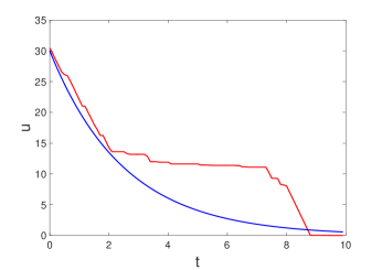
Figure 1: The optimal control for N=30, M=100 and t $\in[0,10]$.

We also compare our solution with the natural cooling which is the traditional annealing control in real chemical experiments. The temperature curve of natural cooling can be approximated as the well-known Newton’s law of cooling. The curve according to Newton’s law of cooling is shown by the red curve in Fig. 1. With the same initial configuration, we run the system (3) under the control of both our numerical solution and the natural cooling, where the Hamiltonian curves and system states are shown in Figs. 2 and 3. These simulations show that our numerical solution has better performance than the natural cooling.

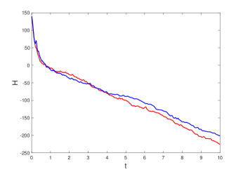
Figure 2: The comparison between our solution and natural cooling. The red line denotes the Hamiltonian curve using the control of our solution, while the blue one is the Hamiltonian curve using the natural cooling control.

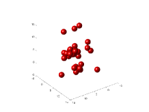
(a) The system state at $t=10$ under the control of natural cooling.

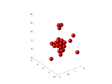
(b) The system state at $t=10$ under the control of our numerical solution.

Figure 3: Simulations of the system (3) with $N=30$.

4 Convergence of noise-free self-assembly model

In this section we consider the noise-free case of our system (3), which can be treated as a multi-agent attractive-repulsive model interested by the study of flocking algorithms (Reynolds, 1987; Olfati-Saber, 2006; Cucker and Dong, 2011). Remark that the interaction between particles in our system is different from the previous works. From (3), the noise-free self-assembly model can be formulated as follows:

$$\left\{\begin{array}[]{l}\dot{X}_{i}=V_{i}\\ \dot{V}_{i}=-BV_{i}+f_{i}\end{array}\right.,~{}~{}1\leq i\leq N.$$ (31)

We give a convergence result for the system (31):

Theorem 1 (Convergence of noise-free model).

Consider the noise-free self-assembly model (31). For any initial state $(X(0),V(0))$, $(X(t),V(t))$ converges to an equilibrium point $(X(\infty),V(\infty))$ which satisfies $V_{i}(\infty)=\mathbf{0}$ and $f_{i}(\infty)=\mathbf{0}$ for all $1\leq i\leq n$.

Proof. The derivative of the Hamiltonian

$$\begin{aligned} \dot{H}&=\frac{1}{2}\sum_{i=1}^{N}\left(\dot{V_{i}^{T}}V_{i}+V_{i}^{T}\dot{V_{i}}\right)+6\sum_{i\neq j}\varepsilon\left(\frac{r_{m}^{6}}{r_{ij}^{7}}-\frac{r_{m}^{12}}{r_{ij}^{13}}\right)\dot{r_{ij}}\\ &=\sum_{i=1}^{N}-BV_{i}^{T}V_{i}+\frac{1}{2}\sum_{i=1}^{N}\left(f_{i}^{T}V_{i}+V_{i}^{T}f_{i}\right)\\ &\ \ +6\sum_{i\neq j}\varepsilon\left(\frac{r_{m}^{6}}{r_{ij}^{8}}-\frac{r_{m}^{12}}{r_{ij}^{14}}\right)\left(X_{i}-X{j}\right)^{T}\left(V_{i}-V_{j}\right)\\ &=\sum_{i=1}^{N}-BV_{i}^{T}V_{i}+\frac{1}{2}\sum_{i=1}^{N}\left(f_{i}^{T}V_{i}+V_{i}^{T}f_{i}\right)\\ &\ \ +\frac{1}{2}\sum_{i=1}^{N}\left(-f_{i}^{T}V_{i}\right)+\frac{1}{2}\sum_{j=1}^{N}\left(-f_{j}V_{j}\right)\\ &=\sum_{i=1}^{N}-BV_{i}^{T}V_{i}\leq 0.\end{aligned}$$ (32)

So the Hamiltonian $H$ will not decrease for any initial state. According to the LaSalle invariance principle, the system will reach the state satisfying $\dot{H}=0$, which is the same as $V_{i}=\mathbf{0}$, so for any initial state we have

$$\lim_{t\to\infty}V_{i}(t)=\mathbf{0}.$$ (33)

It remains to prove $\lim_{t\to\infty}f_{i}(t)=\mathbf{0}$ for any $1\leq i\leq N$. We prove this result by contradiction. If there exists $i\in\{1,\ldots,N\}$ such that $f_{i}(t)$ does not converge to zero, then there exists a constant $\varepsilon>0$, an integer $k\in\{1,2,3\}$, and an infinite sequence $t_{1}<t_{2}<\cdots$ satisfying $t_{j+1}-t_{j}\geq 1$ and

$$|f_{ik}(t_{j})|\geq 2\varepsilon.$$ (34)

By (33), there exists an integer $J>0$ such that

$$|V_{ik}(t_{j})|\leq\frac{1}{B}\varepsilon,~{}~{}~{}~{}\forall j\geq J.$$ (35)

Substituting this into (31) we can get

$$|\dot{V}_{ik}(t_{j})|=|-BV_{ik}(t_{j})+f_{ik}(t_{j})|\geq\varepsilon,~{}~{}~{}~{}\forall j\geq J.$$ (36)

For convenience we omit $t$ in the next part. On the other hand,

$$\begin{aligned} \left\|\ddot{V}_{i}\right\|&=\left\|-B\dot{V}_{i}+\dot{f}_{i}\right\|\\ &=\left\|-B(-BV_{i}+f_{i})+\dot{f}_{i}\right\|\\ &=\left\|B^{2}V_{i}-Bf_{i}+\dot{f}_{i}\right\|\\ &\leq\left\|B^{2}V_{i}\right\|+\left\|Bf_{i}\right\|+\left\|\dot{f}_{i}\right\|\end{aligned}$$ (37)

Because $\lim_{t\to\infty}V_{i}(t)=\mathbf{0}$ , the first part $\left\|B^{2}V_{i}\right\|$ is uniformly bounded. For the second part,

$$\begin{aligned} \left\|Bf_{i}\right\|&=B\left\|\sum_{j\neq i}12\varepsilon\left(\frac{r_{m}^{6}}{r_{ij}^{8}}-\frac{r_{m}^{12}}{r_{ij}^{14}}\right)\left(X_{j}-X_{i}\right)\right\|\\ &=12B\varepsilon\sum_{j\neq i}\left|\frac{r_{m}^{6}}{r_{ij}^{8}}-\frac{r_{m}^{12}}{r_{ij}^{14}}\right|\left\|\left(X_{j}-X_{i}\right)\right\|\\ &=12B\varepsilon\sum_{j\neq i}\left|\frac{r_{m}^{6}}{r_{ij}^{8}}-\frac{r_{m}^{12}}{r_{ij}^{14}}\right|r_{ij}\\ &\leq 12B\varepsilon N\max_{i\neq j}\left|\frac{r_{m}^{6}}{r_{ij}^{7}}-\frac{r_{m}^{12}}{r_{ij}^{13}}\right|\\ \end{aligned}$$ (38)

The limitation of this function of $r_{ij}$ :$\left|\frac{r_{m}^{6}}{r_{ij}^{7}}-\frac{r_{m}^{12}}{r_{ij}^{13}}\right|$ is zero when $r_{ij}\to\infty$. So it is bounded when $r_{ij}$ is large.For another, if $r_{ij}$ is small, we can deduce it has a lower bound using the Hamiltonian $H$. Because $H$ is decreasing. so it will always be smaller than the initial Hamiltonian $H(0)$. And also the two-particle potential has the minimum $-\varepsilon$.$r_{ij}$ will always be subject to

$$\varepsilon\left(\frac{r_{m}^{12}}{r_{ij}^{12}}-2\frac{r_{m}^{6}}{r_{ij}^{6}}\right)+\frac{N(N-1)}{2}(-\varepsilon)\leq H(0)$$ (39)

So the $r_{ij}(t)$ has a positive low bounded, which indicates that the second part $|Bf_{i}(t)|$ of the last line of (37) has a uniform upper bound.

For the third part $\dot{f}_{i}(t)$ of the last line of (37),according to (5), is

$$\begin{aligned} \left\|\dot{f}_{i}(t)\right\|&=12\varepsilon\sum_{j\neq i}\bigg{\|}\left(\frac{r_{m}^{6}}{r_{ij}^{8}}-\frac{r_{m}^{12}}{r_{ij}^{14}}\right)\left(V_{j}-V_{i}\right)\\ &+\left(-8\frac{r_{m}^{6}}{r_{ij}^{9}}+14\frac{r_{m}^{12}}{r_{ij}^{15}}\right)\frac{1}{r_{ij}}\left(X_{j}-X_{i}\right)^{T}\\ &~{}~{}\left(V_{j}-V_{i}\right)\left(X_{j}-X_{i}\right)\bigg{\|}\\ &\leq 12\varepsilon\sum_{j\neq i}\Bigg{|}\left(\frac{r_{m}^{6}}{r_{ij}^{8}}-\frac{r_{m}^{12}}{r_{ij}^{14}}\right)2\sup_{i,t}||V_{i}||\Bigg{|}\\ &+\bigg{|}-8\frac{r_{m}^{6}}{r_{ij}^{9}}+14\frac{r_{m}^{12}}{r_{ij}^{15}}\bigg{|}\cdot 2|r_{ij}|\sup_{i,t}||V_{i}||.\end{aligned}$$ (40)

Because from (33) we get $V_{i}$ has a uniform upper bound, and from (39) we get $r_{ij}$ has a positive low bounded, so by (40) we obtain $|\dot{f}_{i}|$ has a uniform upper bound. Given the discussion above we get $|\ddot{V}_{i}(t)|$ is uniformly bounded.

Since $\dot{V}_{ik}(t)$ is a derivable function, and $\ddot{V}_{ik}(t)$ is uniformly bounded, we can find a constant $\delta>0$ such that

$$|\dot{V}_{ik}(t)-\dot{V}_{ik}(t_{j})|\leq\frac{\varepsilon}{2},~{}~{}~{}\forall j\geq J,t\in[t_{j}-\delta,t_{j}+\delta].$$ (41)

By (41) and (36) we get

$$\begin{aligned} &|V_{ik}(t_{j}+\delta)-V_{ik}(t_{j}-\delta)|\\ &=\Big{|}\int_{t_{j}-\delta}^{t_{j}+\delta}\dot{V}_{ik}(t)dt\Big{|}\geq\delta\varepsilon,~{}~{}\forall j\geq J,\end{aligned}$$ (42)

which is contradictory with (33). $\Box$

We use $20$ particles to simulate the system (31) as follows: Assume the initial positions of all particles are uniformly and independently distributed in $[0,10]^{3}$, and the initial velocities are uniformly and independently distributed in $[0,1]^{3}$. Let $B=1$, $\varepsilon=1$, and $r_{m}=2$. The initial state and final state of the system (31) are shown in Figure 4.

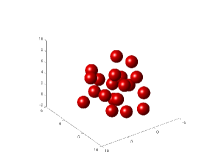
(a) The initial state

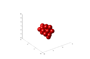
(b) The final state

Figure 4: A simulation for the system (31) with $N=20$.

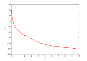
Figure 5: The Hamiltonian $H$ of the system (31) with the same configuration as Fig 4.

5 Conclusion and future works

This paper provides a novel multi-agent model for chemical self-assembly. Because the particles in our model cannot be controlled directly, we propose a optimal temperature control problem which can be treated as a kind of soft control. A numerical method to our optimization problem is explored. Also, we consider the noise-free case of our system and prove its convergence.

The temperature control plays a key role in chemical self-assembly however few mathematical theory exists. In the future we could adjust our model and method according to the real chemical experiment. For example, the force $f_{i}$ could be remodeled according to the dynamics of the assembly particles, and the damping coefficient $B$ could be determined by the kind of the fluid. Another future work could change the objective function in our model according to the requirement of the real chemical experiment. For example, if we want the components assemble a specific structure, we need to choose a suitable objective function to fit the target structure.

References

• Acebrón et al. (2005) Juan A Acebrón, Luis L Bonilla, Conrad J Pérez Vicente, Félix Ritort, and Renato Spigler. The kuramoto model: A simple paradigm for synchronization phenomena. Reviews of modern physics, 77(1):137, 2005.
• Buhl et al. (2006) Jerome Buhl, David JT Sumpter, Iain D Couzin, Joe J Hale, Emma Despland, Edgar R Miller, and Steve J Simpson. From disorder to order in marching locusts. Science, 312(5778):1402–1406, 2006.
• Chen et al. (2017) Ge Chen, Le Yi Wang, Chen Chen, and George Yin. Critical connectivity and fastest convergence rates of distributed consensus with switching topologies and additive noises. IEEE Transactions on Automatic Control, 62(12):6152–6167, 2017.
• Coffey and Kalmykov (2004) William T. Coffey and Yuri P. Kalmykov. The Langevin Equation: With Applications to Stochastic Problems in Physics, Chemistry and Electrical Engineering, 3rd Edition. WORLD SCIENTIFIC, 2004.
• Cucker and Dong (2011) Felipe Cucker and Jiu Gang Dong. A general collision-avoiding flocking framework. IEEE Transactions on Automatic Control, 56(5):1124–1129, 2011.
• Deffuant et al. (2000) Guillaume Deffuant, David Neau, Frederic Amblard, and Gérard Weisbuch. Mixing beliefs among interacting agents. Advances in Complex Systems, 3(01n04):87–98, 2000.
• Gittins et al. (2002) David I Gittins, Andrei S Susha, Bjoern Schoeler, and Frank Caruso. Dense nanoparticulate thin films via gold nanoparticle self-assembly. Advanced Materials, 14(7):508–512, 2002.
• Glasserman (2004) Paul Glasserman. Monte Carlo Methods in Financial Engineering. Springer,, 2004.
• Han et al. (2006) Jing Han, Ming Li, and Lei Guo. Soft control on collective behavior of a group of autonomous agents by a shill agent. Journal of Systems Science and Complexity, 19(1):54–62, 2006.
• Hegselmann et al. (2002) Rainer Hegselmann, Ulrich Krause, et al. Opinion dynamics and bounded confidence models, analysis, and simulation. Journal of artificial societies and social simulation, 5(3), 2002.
• Kaplan (2006) Ilya G Kaplan. Intermolecular interactions: physical picture, computational methods and model potentials. John Wiley & Sons, 2006.
• Klotsa and Jack (2013) Daphne Klotsa and Robert L Jack. Controlling crystal self-assembly using a real-time feedback scheme. The Journal of Chemical Physics, 138(9):094502, 2013.
• Kuramoto (1975) Yoshiki Kuramoto. Self-entrainment of a population of coupled non-linear oscillators. In International Symposium on Mathematical Problems in Theoretical Physics, Lecture Notes in Physics, pages 420–422, 1975.
• Nykypanchuk et al. (2008) Dmytro Nykypanchuk, Mathew M. Maye, Daniel Van Der Lelie, and Oleg Gang. Dna-guided crystallization of colloidal nanoparticles. Nature, 451(7178):549–52, 2008.
• Øksendal (1985) Bernt Øksendal. Stochastic Differential Equations, An introduction with Applications. Springer-Verlag, 1985.
• Olfati-Saber (2006) R. Olfati-Saber. Flocking for multi-agent dynamic systems: algorithms and theory. IEEE Transactions on Automatic Control, 51(3):401–420, 2006.
• Reynolds (1987) Craig W Reynolds. Flocks, herds and schools: A distributed behavioral model. Acm Siggraph Computer Graphics, 21(4):25–34, 1987.
• Service (2005) R. F. Service. How far can we push chemical self-assembly? Science, 309(5731):95, 2005.
• Spellucci (1998) P. Spellucci. An sqp method for general nonlinear programs using only equality constrained subproblems. Mathematical Programming, 82(3):413–448, 1998.
• Vicsek et al. (1995) Tamás Vicsek, András Czirók, Eshel Ben-Jacob, Inon Cohen, and Ofer Shochet. Novel type of phase transition in a system of self-driven particles. Physical review letters, 75(6):1226, 1995.
• Whitesides and Grzybowski (2002) George M. Whitesides and Bartosz Grzybowski. Self-assembly at all scales. Science, 295(5564):2418–2421, 2002.
• Wilber et al. (2009) A. W. Wilber, J. P. Doye, and A. A. Louis. Self-assembly of monodisperse clusters: Dependence on target geometry. Journal of Chemical Physics, 131(17):11B601, 2009.