Form factors for pions couplings to constituent quarks under weak magnetic field

Abstract

By considering a one loop background field method for a nonperturbative one gluon exchange between quarks, leading electromagnetic form factors of pion couplings to constituent quarks are derived by means of from a large quark and gluon effective masses expansion. With this calculation the leading anisotropic corrections induced by a weak magnetic field for the pion- constituent quark form factors are obtained. Besides that, few effective couplings which emerge only due to the weak magnetic field that break chiral and isospin symmetry are also found. Numerical estimations for these magnetic field corrections are presented for two different nonperturbative gluon propagators. All of these corrections are ultraviolet finite and their relative values are found to be of order of $(eB_{0}/{M^{*}}^{2})^{n}$ being $n=1$ for the vector and axial pion couplings and $n=2$ for the pseudoscalar and scalar ones. The corresponding anisotropic corrections to the Strong averaged quadratic radii in the plane perpendicular to the magnetic field are also calculated as functions of the quark effective mass.

1 Introduction

Although lattice QCD is expected to provide the final quantitative answers for the description of hadrons in terms of the more fundamental degrees of freedom it is very interesting to develop analytical tools to describe the gaps between the fundamental level and the measured hadron/nuclear properties. Among these, there are hadrons electromagnetic and strong form factors that make possible a suitable comparison of many important observables calculated theoretically from different approaches, for example [1, 2, 3, 4, 5, 6, 7, 8, 9, 10, 11], with experiments, for example [12, 13, 14, 15, 16]. In particular hadron charge distribution, spin structure and electroweak interaction properties can be understood in terms of electromagnetic and axial form factors. Due to the enormous difficulties in solving QCD in the low energy non perturbative regime, effective models have been developed based on general QCD symmetries and properties and phenomenology, in particular Chiral Symmetry and its Dynamical Symmetry Breaking (DChSB). The constituent quark model (CQM) describes many aspects of phenomenology and it is usually considered to incorporate the pion cloud [17, 18]. A further proposal along these lines is the Weinberg’s large N_c effective field theory (EFT) that copes constituent quark picture with the large N_c expansion [19]. This EFT has been derived in [20, 21] without and with electromagnetic interaction by starting from a quark-quark interaction due to a dressed one gluon exchange. The resulting effective interactions correspond to tree level couplings between pions and constituent quarks. The background quarks, dressed by a sort of gluon cloud described by a non perturbative gluon propagator, yield constituent quarks [22]. One might expect that a comparison between the electromagnetic and strong constituent quark form factors and baryons form factors in the vacuum and at finite energy densities might shed light on diverse aspects of baryons structure and interactions as well as it might provide further criteria to understand or improve the reliability of the CQM to describe low and intermediary energies hadrons. Besides that, one might obtain a systematic way of calculating further effects due to finite energy densities environments.

In the last decade a high interest on the effect of magnetic fields on hadron properties and dynamics increased due to estimates for intense magnetic fields expected to appear in peripheral heavy ions collisions, supernovae and in magnetars [23, 24, 25]. Large magnetic fields, of the order of $(eB_{0})\simeq 10^{17}-10^{19}$G $\simeq(0.1-15)m_{\pi}^{2}$, would not be so large as compared to an hadron mass scale such as the nucleon mass, although it would only appear for a short time interval in non central heavy ions collisions [26]. One cannot expect large magnetic fields in low/intermediary energies hadron collisions in which the usual pion dynamics is expected to be dominant, however pion interactions with photons and their behavior under weak magnetic field might eventually provide observable effects at intermediary energies. Moreover, it has been envisaged nuclear structure changes due to external relatively weak magnetic fields [25] and it becomes important to understand further the magnetic field effects on each part of the nucleon potential among which those dictated by the pion couplings. Many works have shown effects of magnetic field in hadron properties, few examples were given in Refs. [27, 28, 29, 30]. In Refs. [31, 32], Electromagnetic and Strong form factors of light vector and axial mesons coupled to constituent quarks were presented and anisotropic corrections to their quadratic radii were found due to a weak magnetic field. The pion constituent quark Strong form factors in the vacuum were presented in [22] and, in the present work, their leading photon couplings and corresponding weak magnetic field corrections are presented by considering the same formalism. Although one might need strong magnetic fields to describe completely dynamics in magnetars, the (relatively) weak magnetic field allows an analytical treatment that makes explicit magnetic field contributions to Strong interactions observables.

The non perturbative one gluon exchange quark-quark interaction is one of the leading terms of QCD effective action. With the minimal coupling to a background electromagnetic field, it is given by a generating functional that is usually called global color model given by [33, 34, 35]:

$$Z = N\int{\cal D}[\bar{\psi},\psi]\exp\;i\int_{x}\left[\bar{\psi}\left(i\not{D}-m\right)\psi-\frac{g^{2}}{2}\int_{y}j_{\mu}^{b}(x){\tilde{R}}^{\mu\nu}_{bc}(x-y)j_{\nu}^{c}(y)+\bar{\psi}J+J^{*}\psi\right],$$ (1)

Where $\int_{x}$ stands for $\int d^{4}x$, ${\cal D}[\bar{\psi},\psi]$ is the functional measure of integration, $J,J^{*}$ are the quark sources, $g^{2}$ is the quark gluon coupling constant, $a,b...=1,...(N_{c}^{2}-1)$ stands for color in the adjoint representation and the quark sources are written in the last terms. Along the work indices $i,j,k=0,...(N_{f}^{2}-1)$ will be used for isospin indices. The color quark current is given by $j^{\mu}_{a}=\bar{\psi}\lambda_{a}\gamma^{\mu}\psi$, and the sums in color, flavor and Dirac indices are implicit. $D_{\mu}=\partial_{\mu}\delta_{ij}-ieQ_{ij}A_{\mu}$ is the covariant quark derivative with the minimal coupling to photons, with the diagonal matrix $\hat{Q}=diag(2/3,-1/3)$. The quark current masses $m$ will be considered to be the same for $u,d$ quarks. The non perturbative gluon propagator is an external input and it is written as $\tilde{R}^{\mu\nu}_{ab}(x-y)$. It must be a non perturbative one by incorporating to some extent the gluonic non Abelian character and, in particular, it will be required that, with a corrected quark-gluon coupling, it has enough strength to yield dynamical chiral symmetry breaking (DChSB), as it has been found in several approches. Few examples in [3, 36, 37, 38, 39, 40, 41]. In several gauges this kernel can be written in terms of transversal and longitudinal components, as: $\tilde{R}^{\mu\nu}_{ab}(x-y)\equiv\tilde{R}^{\mu\nu}_{ab}=\delta_{ab}\left[\left(g^{\mu\nu}-\frac{\partial^{\mu}\partial^{\nu}}{\partial^{2}}\right)R_{T}(x-y)+\frac{\partial^{\mu}\partial^{\nu}}{\partial^{2}}R_{L}(x-y)\right]$.

The method employed below has been described with details in Refs. [20, 21] and therefore it will be very succintly reminded in the next section. The work is organized as follows. In the next section the determinant of sea quarks is presented for structureless pion field and then it is expanded for large quark effective mass and small electromagnetic field. The complete momentum dependence of the leading electromagnetic effective couplings of pion interactions with constituent quarks are presented as momentum integrals of components of the quark and gluon propagators. Next, a magnetic field, weak with respect to the quark effective mass, is considered. The emergence of anisotropic corrections to pion-constituent quarks couplings are shown. In the following section two non perturbative gluon propagators are considered to provide numerical results, the Tandy-Maris propagator [42] and an effective confining one [38], both of them produce DChSB. The corresponding anisotropic corrections to the Strong (axial and pseudoscalar) quadratic radii due to a weak magnetic field are also presented. In the final section there is a Summary.

2 Constituent quarks and quark-antiquark light mesons

To make possible a more complete investigation of all the flavor channels, a Fierz transformation for the model (1) is performed and only the color singlet terms are considered, being that the color non singlet ones are non leading order at least due to a factor $1/N_{c}$. Chiral structures with combinations of bilocal currents are obtained. The quark field must be responsible for the formation of mesons and baryons and these different possibilities are envisaged by considering the Background Field Method (BFM). Background quark component will be associated to constituent quark ($\psi_{1}$) and the sea quark can be integrated out ($\psi_{2}$). For the one loop BFM it is enough to perform a shift of each of the quark currents obtained from the Fierz transformation. For each of the isospin and Dirac channels the following shift of the bilocal quark currents is perfomed:

$$\bar{\psi}\Gamma^{m}\psi\to(\bar{\psi}\Gamma^{m}\psi)_{2}+(\bar{\psi}\Gamma^{m}\psi)_{1},$$

where $\Gamma^{m}$ are the combinations of Dirac and isospin matrices. The integration of the sea quark is improved with respect to the usual one loop BFM by introducing light quark-antiquark mesons and excitations by means of the auxiliary field method. The following bilocal auxiliary fields, representing quark-antiquark states, are introduced [43], However only the lightest (chiral) scalar and isotriplet pseudoscalar sector will be kept analogous to Ref. [22] and the heavier vector and axial ones will be neglected being less relevant at low energies. The corresponding unity integral for the scalar and pseudoscalar auxiliary bilocal fields $S(x,y),P_{i}(x,y)$ is the following:

$$1 = {\cal N}\int D[S]D[P_{i}]\exp\left(-\frac{i\alpha}{2}\int_{x,y}R(x-y)\left[(S(x,y)-gj^{S}_{(2)}(x,y))^{2}+(P_{i}(x,y)-gj^{P}_{i,(2)}(x,y))^{2}\right]\right),$$ (2)

where $N^{\prime\prime}$ is a normalization, the subscripts ₍₂₎ in the quark currents stand for the corresponding quark component and $R(x-y)=3R_{T}(x-y)+R_{L}(x-y)$. Bilocal auxiliary fields for the different flavors can be expanded in an infinite orthogonal basis with all the excitations in the corresponding channel. For the pseudoscalar isotriplet fields one has:

$$P_{i}(x,y)=P_{i}\left(\frac{x+y}{2},x-y\right)=P_{i}(u,z)=\sum_{k}F_{k}(z)P_{i,k}(u),$$ (3)

where $F_{k}$ are vacuum functions invariant under translation for each of the local field $P^{\mu}_{i,k}(u)$. At lower energies, the lowest energy modes, lighest $k=0$ will be kept, i.e. $P_{i,k=0}=\pi_{i}$ that are the pions. The form factors reduce to constants in the zero momentum and structureless limit $F_{k}(z)=F_{k}(0)$. This is obtained by expanding bilocal fields in an infinite orthogonal basis for all the excitations of a given channel, for example for the pseudoscalar isotriplet fields one has: $P_{i}(x,y)=P_{i}\left(\frac{x+y}{2},x-y\right)=P_{i}(u,z)=\sum_{k}F_{k}(z)P_{i,k}(u)$, where $F_{k}(z)$ are vacuum functions invariant under translation for each of the local field $P_{i,k}(u)$. Only the lowest energy modes, lighest $k=0$ can be expected to contribute in the low energy regime. In the pseudoscalar channel it corresponds to dimensionless pion field: $P_{i,k=0}=\pi_{i}$, and their form factors reduce to constants $F_{k}(z)=F_{k}(0)$ endowing the fields with their canonical normalization. The (heavier) vector and axial mesons with their couplings to the constituent quarks were considered in [31, 32] and they can be neglected in the lower energy regime indeed. With that, by integrating out the sea quarks, the background photon couplings to light mesons and constituent quarks arise. The auxiliary fields are undetermined and the corresponding saddle point equations can be used for this. In the mean field they can be written from the conditions:

$$\frac{\partial S^{eff}_{af}}{\partial\phi_{\alpha}}=0,$$ (4)

where $S^{eff}_{af}$ is the effective action obtained with the integration of the sea quark with the auxiliary fields and $\phi_{\alpha}$ stands for each of the (constant) auxiliary fields. These equations for the NJL model and for the model (1) have been analyzed in many works in the vacuum or under finite energy densities. In the vacuum, the scalar auxiliary field is the only one whose gap equation has a non trivial solution corresponding to a scalar quark-antiquark condensate as the order parameter of DChSB. At non zero constant magnetic fields a contribution to the quark effective mass arises associated to the so called magnetic catalysis that is well established from NJL-type and other models and also lattice QCD. The scalar quark-antiquark field does not necessarily correspond to a light meson and a chiral rotation can be performed by freezing this degree of freedom. Pion field will be described by means of the collective variables: $U,U^{\dagger}=e^{i\vec{\sigma}\cdot\vec{\pi}},e^{-i\vec{\sigma}\cdot\vec{\pi}}$.

The sea quark determinant yields the dynamics of the mesons fields with their couplings to constituent quarks, and it can be written as [20, 21]:

$$S_{det} = -i\;Tr\;\ln\;\left\{iS_{c,q}^{-1}(x-y)\right\},$$ (5)

$$S_{c,q}^{-1}(x-y) \equiv S_{0,c}^{-1}(x-y)+\Xi_{s}(x-y)+\sum_{q}a_{q}\Gamma_{q}j_{q}(x,y),$$ (6)

where $Tr$ stands for traces of all discrete internal indices and integration of spacetime coordinates and $\Xi_{s}(x-y)$ stands for the coupling of sea quark to the pions. It can be written:

$$\Xi_{s}(x-y) = F(P_{R}U+P_{L}U^{\dagger})\;\delta(x-y),$$ (7)

where $P_{R/L}=(1\pm\gamma_{5})/2$ are the chiral right/left hand projectors and $F$ the pion field normalization constant. The quark kernel can be written in terms of the effective quark mass generated by the scalar field gap equation as

$$S_{0,c}^{-1}(x-y)=\left(i\not{D}-M^{*}\right)\delta(x-y).$$ (8)

In expression (6) the following quantity with the color singlet chiral constituent quark currents has been defined:

$$\frac{\sum_{q}a_{q}\Gamma_{q}j_{q}(x,y)}{\alpha g^{2}} = 2R(x-y)\left[\bar{\psi}(y)\psi(x)+i\gamma_{5}\sigma_{i}\bar{\psi}(y)i\gamma_{5}\sigma_{i}\psi(x)\right]$$ (9)

$$- \bar{R}^{\mu\nu}(x-y)\gamma_{\mu}\sigma_{i}\left[\bar{\psi}(y)\gamma_{\nu}\sigma_{i}\psi(x)+\gamma_{5}\bar{\psi}(y)\gamma_{5}\gamma_{\nu}\sigma_{i}\psi(x)\right],$$

In this expression $\alpha=2/9$, for flavor SU(2) and color SU(3), and combinations of the longitudinal and transversal parts of the gluon propagator were defined as:

$$R{(x-y)} = 3R_{T}(x-y)+R_{L}(x-y),$$ (10)

$$\bar{R}^{\mu\nu}{(x-y)} = g^{\mu\nu}(R_{T}(x-y)+R_{L}(x-y))+2\frac{\partial^{\mu}\partial^{\nu}}{\partial^{2}}(R_{T}(x-y)-R_{L}(x-y)).$$

With the background quark currents, different quark-couplings were found to emerge in the large quark and gluon effective masses expansion of the above determinant. The leading term is an effective (Lagrangian) constituent quark mass that turns out to provide a running quark mass with very similar momentum structure to the running quark mass from elaborated SDE at the rainbow ladder level as shown in [22]. This effective mass however is not the same as the gap quark effective mass and it does not depend on DChSB, being seemingly akin to other mechanisms [44].

3 Leading Electromagnetic form factors

The large effective quark mass expansion of the determinant within the zero order derivative expansion is performed in the following. The leading momentum dependent couplings with the background electromagnetic field are the following:

$${\cal L}^{q-\pi}_{A} = F_{s,\gamma}(K,Q,Q_{1},Q_{3})\;F_{\mu\nu}(Q_{1})F^{\mu\nu}(Q_{3}){\pi}_{i}(q_{a})\pi_{i}(q_{b})\;\bar{\psi}(K)\psi(K+Q+Q_{1}+Q_{3})$$ (11)

$$+ F_{ps,\gamma}(K,Q,Q_{1},Q_{3})\;F_{\mu\nu}(Q_{1})F^{\mu\nu}(Q_{3})\epsilon_{ij3}\pi_{i}(Q_{1})\;\bar{\psi}(K)\sigma_{j}i\gamma_{5}\psi(K+Q+Q_{1}+Q_{3})$$

$$+ T_{jki}F_{V,\gamma}(K,Q,Q_{1})\;F^{\mu\nu}(Q_{1})\pi_{j}(q_{a})(\partial_{\mu}\pi_{k}(q_{b}))\bar{\psi}(K)\gamma_{\mu}\sigma^{i}\psi(K+Q+Q_{1})$$

$$+ \epsilon_{ij3}F_{A,\gamma}(K,Q,Q_{1})\;F^{\mu\nu}(Q_{1})\;\partial_{\mu}\pi_{i}(Q)\;\bar{\psi}(K)i\gamma_{5}\gamma_{\nu}\sigma^{j}\psi(K+Q+Q_{1}),$$

where in the couplings with two pions $Q=q_{a}+q_{b}$. The form factors in this expression are given by:

$$F_{s,\gamma}(K,Q,Q_{1},Q_{3}) = \frac{80}{9}d_{1}N_{c}(\alpha g^{2})e^{2}FF_{4}^{t}(K,Q,Q_{1},Q_{3}),$$ (12)

$$F_{ps,\gamma}(K,Q,Q_{1},Q_{3}) = \frac{64}{3}d_{1}N_{c}(\alpha g^{2})e^{2}\;FF_{4}^{t}(K,Q,Q_{1},Q_{3}),$$ (13)

$$F_{V,\gamma}(K,Q,Q_{1}) = \frac{64}{3}d_{1}N_{c}F(\alpha g^{2})e\;F_{5}^{t}(K,Q,Q_{1}),$$ (14)

$$F_{A,\gamma}(K,Q,Q_{1}) = \frac{64}{3}d_{1}N_{c}F(\alpha g^{2})e\;F_{5}^{t}(K,Q,Q_{1}).$$ (15)

In this leading order of the determinant expansion, there are also unusual or anomalous couplings to the electromagnetic field that also break chiral and isospin symmetries explicitely and that correspond to sort of mixing couplings induced by the photon. The leading ones can be written as:

$${\cal L}_{Aj} = -i\epsilon_{ij3}F{F}_{6P}(K,Q,Q_{1})A_{\mu}(Q_{1})(\partial^{\mu}\pi_{i}(q_{a}))\pi_{j}(q_{b})\;\bar{\psi}(K)\psi(Q_{T})$$ (16)

$$- 2i\epsilon_{ij3}F{F}_{6M}(K,Q,Q_{1})A_{\mu}(Q_{1})\partial^{\mu}\pi_{i}(Q)\;\bar{\psi}(K)i\gamma_{5}\sigma^{j}\psi(Q_{T})$$

$$+ iJ_{ijk}F{F}_{7P}(K,Q,Q_{1})A_{\mu}(Q_{1})\;\pi_{i}(q_{a})\pi_{j}(q_{b})\;\;\bar{\psi}(K)i\gamma^{\mu}\sigma^{k}\psi(Q_{T})$$

$$+ 2i\epsilon_{ji3}F{F}_{7M}(K,Q,Q_{1})A_{\mu}(Q_{1})\pi_{j}(Q)\;\bar{\psi}(K)i\gamma^{\mu}\gamma_{5}\sigma^{j}\psi(Q_{T}),$$

where $J_{ii3}=J_{3ii}=-J_{i3i}=1$, for $i=1,2$, and $J_{ijk}=\frac{i}{3}\epsilon_{ijk}$ for $i\neq j\neq k$. The form factors were defined in terms of functions $H_{6P,M}$ and $H_{7P,M}$:

$${F}_{6P}(K,Q,Q_{1}) = 4d_{1}eN_{c}K_{0}H_{6P}^{t}(K,Q,Q_{1}),$$ (17)

$$F_{6M}(K,Q,Q_{1}) = 4d_{1}eN_{c}K_{0}H_{6M}^{t}(K,Q,Q_{1}),$$ (18)

$${F}_{7P}(K,Q,Q_{1}) = 4d_{1}eN_{c}K_{0}H_{7P}^{t}(K,Q,Q_{1}),$$ (19)

$${F}_{7M}(K,Q,Q_{1}) = 4d_{1}eN_{c}K_{0}H_{7M}^{t}(K,Q,Q_{1}).$$ (20)

The functions $F_{i}^{t}(K,Q,Q_{1})$, $H_{i}^{t}(K,Q,Q_{j})$ used above were defined as:

$$F_{3}^{t}(K,Q,Q_{1}) = \frac{1}{2}\left(F_{3}(K,Q,Q_{1})+F_{3}(k,Q_{1},Q)\right),$$

$$F_{4}^{t}(K,Q,Q_{1},Q_{3}) = \frac{1}{2}\left(F_{4}(K,Q,Q_{1},Q_{3})+\tilde{F}_{4}(K,Q_{3},Q_{1},Q)\right),$$

$$F_{5}^{t}(K,Q,Q_{1}) = \frac{1}{2}\left(F_{5}(K,Q,Q_{1})+F_{5}(K,Q_{1},Q)\right),$$

$${H}_{6P}^{t}(K,Q,Q_{1}) = \frac{1}{2}\left({F}_{6}(K,Q,Q_{1})+{F}_{6}(K,Q_{1},Q)\right),$$ (21)

$${H}_{6M}^{t}(K,Q,Q_{1}) = \frac{1}{2}\left({F}_{6}(K,Q,Q_{1})-{F}_{6}(K,Q_{1},Q)\right),$$ (22)

$${H}_{7P}^{t}(K,Q,Q_{1}) = \frac{1}{2}\left({F}_{7}(K,Q,Q_{1})+{F}_{7}(K,Q_{1},Q)\right),$$ (23)

$${H}_{7M}^{t}(K,Q,Q_{1}) = \frac{1}{2}\left({F}_{7}(K,Q,Q_{1})-{F}_{7}(K,Q_{1},Q)\right).$$ (24)

In these expressions the loop momentum integrals of each of the form factors can be written in Euclidean momentum space, always for incoming quark momentum $K=0$, as:

$$F_{3}(0,Q,Q_{1}) = \int_{k}\left[k\cdot(k+Q_{1})-{M^{*}}^{2}\right]\tilde{S}_{0}(k)\tilde{S}_{0}(k+Q_{1})\tilde{S}_{0}(k+Q+Q_{1})\bar{\bar{R}}(-k),$$ (25)

$$F_{4}(0,Q_{1},Q,Q_{3}) = \int_{k}\left[-k\cdot(k+Q_{1}+Q)+{M^{*}}^{2}\right]\tilde{S}_{0}(k)\tilde{S}_{0}(k+Q_{1}+Q)\tilde{S}_{0}(k+Q_{1})\tilde{S}_{0}(k+Q_{4})R(-k),$$ (26)

$$\tilde{F}_{4}(0,Q,Q_{1},Q_{3}) = \int_{k}\left[k^{2}+k\cdot Q-{M^{*}}^{2}\right]\tilde{S}_{0}(k)\tilde{S}_{0}(k+Q)\tilde{S}_{0}(k+Q+Q_{1})\tilde{S}_{0}(k+Q_{4})R(-k),$$ (27)

$$F_{5}(0,Q,Q_{1}) = \int_{k}M^{*}\tilde{S}_{0}(k)\tilde{S}_{0}(k+Q_{1})\tilde{S}_{0}(k+Q+Q_{1})\bar{\bar{R}}(-k),$$ (28)

$$F_{6}(0,Q,Q_{1}) = \int_{k}\left[k\cdot(k+Q+Q_{1})-{M^{*}}^{2}\right]\tilde{S}_{0}(k)\tilde{S}_{0}(k+Q_{1})\tilde{S}_{0}(k+Q+Q_{1}){R}(-k),$$ (29)

$$F_{7}(0,Q,Q_{1}) = \int_{k}\left[3k^{2}+k\cdot(4Q_{1}+2Q)+Q_{5}-{M^{*}}^{2}\right]\tilde{S}_{0}(k)\tilde{S}_{0}(k+Q_{1})\tilde{S}_{0}(k+Q+Q_{1})\bar{R}(-k),$$ (30)

where $Q_{4}=Q_{1}+Q+Q_{3}$, $Q_{5}=Q_{1}^{2}+Q\cdot Q_{1}$, $\int_{k}=\int\frac{d^{4}k}{(2\pi)^{4}}$ and $\bar{\bar{R}}(k)=2R(k)$. The following function was used: $\tilde{S}_{0}(k)=\frac{1}{k^{2}+{M^{*}}^{2}}$.

The complete momentum structure of form factors such as $F_{3}$ and $F_{4}$ present a non monotonic behavior that is not observed experimental data and they yield negative averaged quadratic radii [31]. To mend this behavior the resulting momentum dependence of the quark kernel will be truncated by the following approximation:

$$S_{0}^{tr}(k)\sim M^{*}\tilde{S}_{0}(k).$$ (31)

It yields truncated form factors with monotonic behavior with pion momenta that make possible to obtain always positive quadratic mean radii at this level. This truncation scheme might be equivalent to consider a momentum dependent quark effective mass $M^{*}$. Because of that, in the present work only the truncated form factors will be investigated numerically.

Figure 1: Diagrams (1a,1b,1c,1d) correspond to the couplings of expressions (11,16). The wavy line with a full dot is a (dressed) non perturbative gluon propagator, the solid lines stand for quarks, dashed lines for pions and the dotted line stands for the photon strength tensor. A full square in a vertex represent momentum dependent pion coupling. The momenta of each of the particles are indicated by $K$ (quarks), $Q$ (pion(s)) and $Q_{1}$ (photons).

The diagrams for expressions (11,16) are presented in Fig. (1). The incoming constituent quark has momentum $K$ and $K+Q_{T}$ is the outgoing constituent quark momentum, where $Q_{T}$ is the total momentum transfered by the pion(s) and photon(s) to the constituent quark. $Q$ denotes the total transfered momentum from the pion(s) and $Q_{1},Q_{3}$ are each of the photon momenta.

4 Weak magnetic field

It is shown now that corrections induced by a weak background magnetic field to those usual form factors are obtained by considering two different effects. Firstly the leading correction to the quark kernel and also by assuming the weak magnetic field (with respect to the constituent quark mass) is strong enough to show up in the electromagnetic couplings of the previous section. For that, the Landau gauge will be considered in which $A^{\mu}=-B_{0}\;(0,0,x,0)$.

The leading quark propagator dependence on the weak magnetic field, for equal up and down quark effective masses $M^{*}$, will not be derived in this work and it can be written as [45, 46]:

$$G(k) = S_{0}(k)+S_{1}(k)(eB_{0})=\frac{\not{k}+M^{*}}{k^{2}-{M^{*}}^{2}}+i\gamma_{1}\gamma_{2}\frac{(\gamma_{0}k^{0}-\gamma_{3}k^{3}+M^{*})}{(k^{2}-{M^{*}}^{2})^{2}}\hat{Q}(eB_{0}).$$ (32)

By substituting the vacuum quark propagator by a $G(k)$ different anisotropic weak magnetic field-dependent corrections to pion constituent quark couplings appear. For some of the leading pion-constituent quark couplings found in [22] however the first order correction to the quark propagator $S_{1}(k)$ does not contribute in the leading terms, i.e. linear in $(eB_{0})$. In the second order in $(eB_{0})^{2}$ more terms arise but this will not be considered below.

The correction $S_{1}(k)$ to the quark propagator yield the following anisotropic contributions from the leading order determinant for the axial constituent quark current expansion:

$${\cal L}_{S,B} = G_{A,1}^{B}\;\epsilon^{0\rho\mu 3}\;\partial_{\mu}\pi_{i}\;\bar{\psi}\gamma_{5}\gamma_{\rho}\sigma_{i}\psi$$ (33)

$$+ G_{V,1}^{B}\;\epsilon^{12\mu\rho}\;\left(\delta_{ij}+\frac{i}{3}\epsilon_{ijk}\right)\partial_{\mu}(\pi_{i}\pi_{j})\;\bar{\psi}\gamma_{5}\gamma_{\rho}\sigma_{j}\psi+G_{V,2}^{B}\;\partial_{0}\pi_{i}\;\bar{\psi}\gamma_{z}\sigma_{j}\psi,,$$

where $\epsilon^{\nu\sigma\mu\rho}$ is the Levi Civita tensor, $\partial_{0}$ stands for $\partial/\partial t$, and the effective coupling constants were defined with the trace of internal indices as:

$$\frac{G_{A,1}^{B}}{\left(\frac{eB_{0}}{{M^{*}}^{2}}\right)}=\frac{2}{3}\frac{G_{V,1}^{B}}{\left(\frac{eB_{0}}{{M^{*}}^{2}}\right)}=\frac{1}{6}\frac{G_{V,2}^{B}}{\left(\frac{eB_{0}}{{M^{*}}^{2}}\right)} = \frac{8}{3}d_{1}N_{c}\;F{M^{*}}^{2}\;(\alpha g^{2})\;F_{5}^{t}(0,Q,0),$$ (34)

where $F_{5}^{t}(0,Q,0)$ is given above in expressions (3,28). The last two terms in the second line of (33) are anomalous since they are not usual Lorentz scalar but pseudoscalar.

Other leading contributions, however, arise from the zeroth order quark propagator of expression (32), $S_{0}(k)$ and a background photon. By considering the pion momentum $Q$, or $Q=q_{a}+q_{b}$ for the two-pion couplings, the resulting anisotropic corrections to pion-constituent quark form factors are obtained from expressions (11), They are given by:

$${\cal L}^{q-\pi}_{B} = F_{s}^{B}(K,Q)F{\pi}_{i}(q_{a})\pi_{i}(q_{b})\;\bar{\psi}(K)\psi(K+Q)$$ (35)

$$+ \epsilon_{ij3}F_{ps}^{B}(K,Q)F\pi_{i}(Q)\;\bar{\psi}(K)\sigma_{j}i\gamma_{5}\psi(K+Q)$$

$$+ T_{jki}F_{V}^{B}(K,Q)\pi_{j}(q_{a})(\partial_{\mu}\pi_{k}(q_{b}))\bar{\psi}(K)\gamma_{\mu}\sigma^{i}\psi(K,Q)$$

$$+ \epsilon_{ij3}\;F_{A}^{B}(K,Q)\;\partial_{\mu}\pi_{i}(Q)\;\bar{\psi}(K)i\gamma_{5}\gamma_{\nu}\sigma^{j}\psi(K,Q),$$

where $T_{jki}=\delta_{ij}\delta_{3k}-\delta_{j3}\delta_{ik}$ and

$$F_{ps}^{B}(K,Q)=\frac{12}{5}F_{s}^{B}(K,Q) = \left(\frac{eB_{0}}{{M^{*}}^{2}}\right)^{2}\frac{64}{3}d_{1}N_{c}{M^{*}}^{4}(\alpha g^{2})\;F_{4}(K,Q,Q_{1}=Q_{3}=0),$$ (36)

$$F_{A}^{B}(K,Q)=\frac{F^{B}_{V}}{3}(K,Q) = \left(\frac{eB_{0}}{{M^{*}}^{2}}\right)\frac{64}{3}d_{1}N_{c}F{M^{*}}^{2}(\alpha g^{2})\;F_{5}(K,Q,Q_{1}=0).$$ (37)

The slightly more symmetric way of defining the magnetic field $A^{\mu}=-B_{0}(0,y,x,0)/2$ garantees the anysotropies to be kept in the plane perpendicular to the magnetic field. The quark effective mass $M^{*}$ receives corrections from the weak magnetic field in the scalar gap equation and it will not addressed with details in the present work. These expressions provide numerical values one order of magnitude smaller than of the original pion - constituent quark couplings because they have multiplicative extra factors $B_{0}$ or $B_{0}^{2}$ that can be factorized in constants such as as $eB_{0}/{M^{*}}^{2}$ or $(eB_{0})^{2}/{M^{*}}^{4}$ within the current large quark effective mass regime. These make explicit that the $B_{0}$ induced corrections are considerably smaller than the original coupling constants and form factors.

The anomalous electromagnetic pion-quark couplings from expression (16) generate magnetic field induced mixing pion couplings breaking explicitely chiral and isospin symmetries. For pion momentum $Q$, or $Q=q_{a}+q_{b}$ in the two pion couplings, it yields:

$${\cal L}_{Aj} = -i\epsilon_{ij3}{F}_{6PB}(K,Q)(\partial^{y}\pi_{i}(q_{a}))\pi_{j}(q_{b})\;\bar{\psi}(K)\psi(K+Q)$$

$$- 2i\epsilon_{ij3}{F}_{6MB}(K,Q)\partial^{y}\pi_{i}(Q)\;\bar{\psi}(K)i\gamma_{5}\sigma^{j}\psi(K+Q)$$

$$+ iJ_{ijk}{F}_{7PB}(K,Q)\;\pi_{i}(q_{a})\pi_{j}(q_{b})\;\;\bar{\psi}(K)i\gamma^{2}\sigma^{k}\psi(K+Q)$$

$$+ 2i\epsilon_{ji3}{F}_{7MB}(K,Q)\pi_{j}(Q)\;\bar{\psi}(K)i\gamma^{2}\gamma_{5}\sigma^{j}\psi(K+Q).$$

The following functions were used in expressions (4) written in terms of the momentum derivative $\partial_{Q_{1,x}}=\partial/\partial Q^{x}_{1}$:

$$F_{6BP}(0,Q) = \left(\frac{eB_{0}}{{M^{*}}^{2}}\right)4d_{1}FN_{c}{M^{*}}^{2}K_{0}\left(\partial_{Q_{1,x}}\;H_{6P}^{t}(0,Q,Q_{1})\right)_{Q_{1}=0},$$ (39)

$$F_{6BM}(0,Q) = \left(\frac{eB_{0}}{{M^{*}}^{2}}\right)4d_{1}FN_{c}{M^{*}}^{2}K_{0}\;\left(\partial_{Q_{1,x}}H_{6M}^{t}(0,Q,Q_{1})\right)_{Q_{1}=0},$$ (40)

$$F_{7BP}(0,Q) = \left(\frac{eB_{0}}{{M^{*}}^{2}}\right)4d_{1}FN_{c}{M^{*}}^{2}K_{0}\;\left(\partial_{Q_{1,x}}H_{7P}^{t}(0,Q,Q_{1})\right)_{Q_{1}=0},$$ (41)

$$F_{7MP}(0,Q) = \left(\frac{eB_{0}}{{M^{*}}^{2}}\right)4d_{1}FN_{c}{M^{*}}^{2}K_{0}\;\left(\partial_{Q_{1,x}}H_{7M}^{t}(0,Q,Q_{1})\right)_{Q_{1}=0}.$$ (42)

By comparing expressions (34) and (37) the following exact ratios are obtained:

$$\frac{G_{A,1}^{B}(0,0)}{F_{A}^{B}(0,0)}=2\frac{G_{V,1}^{B}(0,0)}{F_{V}^{B}(0,0)}=\frac{G_{V,1}^{B}(0,0)}{G_{V,2}^{B}(0,0)}=\frac{1}{8}.$$ (43)

These ratios are simple numerical factors and the momentum dependence of only one of these form factors, $F_{A}^{B}(K,Q)$, will be explicitely shown below.

4.1 Numerical results

In the following, numerical estimations for the form factors above will be shown. Two gluon propagators will be considered, firstly a transversal one from Tandy-Maris $D_{I}(k)$ [42] and the other is an effective confining longitudinal one by Cornwall $D_{II}(k)$ [38]. Both of them yield DChSB in the gap equation for the scalar auxiliary field being that:

$$g^{2}\tilde{R}^{\mu\nu}(k)\equiv h_{a}D_{a}^{\mu\nu}(k),$$ (44)

where $D^{\mu\nu}_{a}(k)$ ($a=I,II$) are the chosen gluon propagators whose expressions are the following:

$$D_{I}(k) = \frac{8\pi^{2}}{\omega^{4}}De^{-k^{2}/\omega^{2}}+\frac{8\pi^{2}\gamma_{m}E(k^{2})}{\ln\left[\tau+(1+k^{2}/\Lambda^{2}_{QCD})^{2}\right]},$$ (45)

$$D_{II}(k) = K_{F}/(k^{2}+M_{k}^{2})^{2},$$ (46)

where for the first expression $\gamma_{m}=12/(33-2N_{f})$, $N_{f}=4$, $\Lambda_{QCD}=0.234$GeV, $\tau=e^{2}-1$, $E(k^{2})=[1-exp(-k^{2}/[4m_{t}^{2}])/k^{2}$, $m_{t}=0.5GeV$, $\omega=0.5$GeV, $D=0.55^{3}/\omega$ (GeV²); and for the second expression $K_{F}=(2\pi M_{k}/(3k_{e}))^{2}$ where $k_{e}=0.15$ and $M_{k}=220$MeV. In expression (44) $h_{a}$ is a constant factor already considered in previous works [21, 32, 22] to fix the quark gluon (running) coupling constant such as to reproduce a particular value for one of the resulting effective coupling constant, for example the pion axial coupling constant $g_{A}h_{a}=1$ or the rho constituent quark coupling constant $g_{\rho}h_{a}\simeq 12$. In the present work they were fixed with the same convention of the pion constituent quark form factors of Ref. [22] for each of the gluon propagators, $h_{I}=0.82$ and $h_{II}=0.3$ .

In figure (2) the axial form factor $F^{B}_{A}(K,Q)/(eB_{0}/{M^{*}}^{2})$ is shown as function of the pion momentum $Q=|Q|$ for two different quark effective mass $M^{*}$ This contribution for the form factor in the figure is divided by a factor $(eB_{0})/{M^{*}}^{2}$ to make easier the interpretation and the comparison of each of the contributions for any small value of $(eB_{0})/{M^{*}}^{2}$. The effective mass $M^{*}$ is, however, kept constant. At zero pion momentum $Q=0$ the form factor yields the axial pion coupling to constituent quark that is usually considered to be $g_{A}=0.8$ or $1$ [6, 19]. Therefore, without further assumptions about the quark-gluon coupling constant, the weak magnetic field correction to the axial form factor is smaller for the gluon propagator $D_{II}(k)$ than for $D_{I}(k)$ and this is simply due to the overal strength of the corresponding propagator and quark-gluon coupling constant.

Figure 2: In this figure the leading magnetic field correction to the axial form factor $F_{A}^{B}(0,Q)/(eB_{0}/{M^{*}}^{2})$ as a function of the pion momentum for the usual pion field is presented for the two gluon propagators $D_{I}(k)$ (thin lines) and $D_{II}(k)$ (thick lines). Different values of the quark effective mass are considered $M^{*}=350$MeV in dot-dashed lines, $M^{*}=310$MeV in dashed lines. $h_{I}=0.82$ and $h_{II}=0.3$

In figure (3) the weak magnetic field anisotropic correction to the pseudoscalar form factor, divided by $(eB_{0}/{M^{*}}^{2})^{2}$, is presented for the two gluon propagators as a function of the pion momentum and for different values of $M^{*}$. Although the value of the pseudoscalar coupling constant is of the order of 10 times the value of the axial coupling constant the weak magnetic field corrections calculated in these figures are basically of the same order of magnitude.

A complete expression for the axial and pseudoscalar form factors, including both their values in the vacuum and the weak $B_{0}$ correction, can be written as

$$G_{A}^{B}(Q) = G_{A}^{M^{*}}(Q)\;+\;\frac{eB_{0}}{{M^{*}}^{2}}\frac{F_{A}^{B}(0,Q)}{(eB_{0}/{M^{*}}^{2})}.$$ (47)

$$G_{ps}^{B}(Q) = G_{ps}^{M^{*}}(Q)\;+\;\left(\frac{eB_{0}}{{M^{*}}^{2}}\right)^{2}\frac{F_{ps}^{B}(0,Q)}{(eB_{0}/{M^{*}}^{2})^{2}}.$$ (48)

Where $G_{A}^{M^{*}}(Q)$ is the form factor presented and investigated in [22], $G_{A}^{M^{*}}(Q)=G_{A}^{U}(0,Q)$, and similarly $G_{ps}^{M^{*}}(Q)=G_{ps}(0,Q)$. In figure (4) the axial and pseudoscalar non truncated form factors in the vacuum - from [22] - and with a weak magnetic field $eB_{0}/{M^{*}}^{2}=0.2$ from expressions (47,48) are presented for the two gluon propagators with an unique value of the quark effective mass $M^{*}=0.31$GeV. Note however the $B_{0}$ correction to the pseudoscalar form factor has a factor $\left(\frac{eB_{0}}{{M^{*}}^{2}}\right)^{2}$ that is considerably smaller than $\left(\frac{eB_{0}}{{M^{*}}^{2}}\right)$ in the axial form factor.

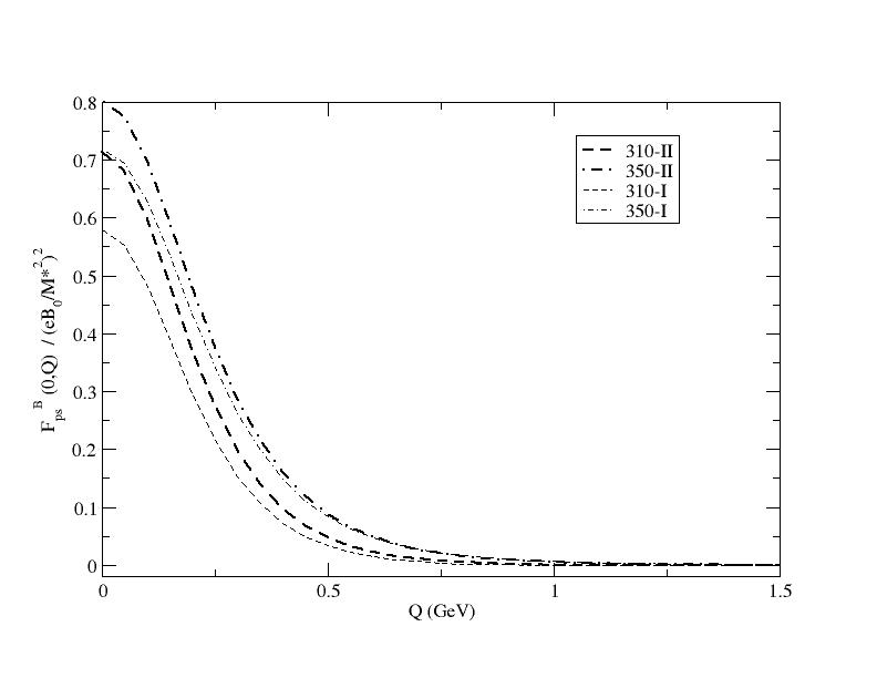
Figure 3: In this figure the leading magnetic field correction to the pseudoscalar form factor $F_{ps}^{B}(0,Q)/(eB_{0}/{M^{*}}^{2})^{2}$ as a function of the pion momentum for the usual pion field is presented for the two gluon propagators $D_{I}(k)$ (thin lines) and $D_{II}(k)$ (thick lines). Different values of the sea quark effective mass are considered $M^{*}=350$MeV in dot-dashed lines, $M^{*}=310$MeV in dashed lines. $h_{I}=0.82$ and $h_{II}=0.3$

Figure 4: Pseudoscalar and axial (non truncated) form factors for $B_{0}=0$, from [22], and for $(eB_{0}/{M^{*}}^{2})=0.2$ with different contributions: from the quark mass dependence on the weak magnetic field and from the correction to the form factor from expressions (47,48) for the two gluon propagators $D_{I}(k)$ and $D_{II}(k)$ and with $M^{*}=310$MeV. $h_{I}=0.82$ and $h_{II}=0.3$.

The unusual weak magnetic field induced anisotropic form factors, $F_{6PB}(0,Q)$ and $F_{7PB}(0,Q)$, are exhibitted in figure (5) as function of the pion momentum , $Q=|Q_{x}|$, for the two gluon propagators with $M^{*}=310$MeV. They disappear in the zero pion momentum limit. The dependence of the form factor $F_{7PB}(0,Q)$ on the gluon propagator is seemingly larger than for the previous form factors analysed in the present work. Although the order of magnitude might be larger than the corresponding electromagnetic form factors (16) these values must be multiplied by $(eB_{0})/{M^{*}}^{2}$.

Figure 5: The leading magnetic field induced form factors for the pion coupling to quark currents $F_{6P-B}(0,Q),F_{7P-B}(0,Q)$, divided by $(eB_{0})/{M^{*}}^{2}$, as functions of the pion momentum, $Q=|Q_{x}|$, are presented for the two gluon propagators $D_{I}(k)$ (thin lines) and $D_{II}(k)$ (thick lines) and $M^{*}=310$MeV. $h_{I}=0.82$ and $h_{II}=0.3$

4.2 Averaged quadratic radii

From the above form factors, weak-$B_{0}$ induced anisotropic corrections to the axial and pseudoscalar constituent quark averaged quadratic radii (a.q.r.) can be obtained. The magnetic field along the $\hat{z}$ direction can be chosen to be $A_{\mu}=-B_{0}(0,y,x,0)/2$ for which it can be obtained a symmetrized result. Because the $B_{0}$ corrections to the form factors are dimensionless as defined above, the a.q.r. can be defined simply as:

$$\Delta<r^{2}>_{A} = \left.-6\;\frac{dF_{A}^{B}(0,Q_{\pi})}{dQ^{2}_{\pi}}\right|_{Q_{\pi}=0},$$

$$\Delta<r^{2}>_{ps} = \left.-6\;\frac{dF_{ps}^{B}(0,Q_{\pi})}{dQ^{2}_{\pi}}\right|_{Q_{\pi}=0}.$$ (49)

that correspond to corrections in the plane $x-y$ perpendicular to the constant weak magnetic field. The corresponding a.q.r. in the vacuum by considering the same method have been presented in Ref. [22]. The resulting value for the axial and pseudoscalar square radii are obtained by adding their values in the vacuum to the magnetic field correction. The quark effective mass $M^{*}$ however is kept constant in spite of its eventual magnetic field dependence. These values are obtained by:

$$<r^{2}>_{A}^{B} = <r^{2}>_{A}+\left.\left(\frac{eB_{0}}{{M^{*}}^{2}}\right)\frac{\Delta<r^{2}>_{A}}{(eB_{0}/{M^{*}}^{2})}\right|_{x-y},$$ (50)

$$<r^{2}>_{ps}^{B} = <r^{2}>_{ps}+\left.\left(\frac{eB_{0}}{{M^{*}}^{2}}\right)^{2}\frac{\Delta<r^{2}>_{ps}}{(eB_{0}/{M^{*}}^{2})^{2}}\right|_{x-y},$$ (51)

where it was emphasized the magnetic field corrections stand only in the plane perpendicular to the weak constant magnetic field. There are corrections to the (strong) vector and scalar square radii that are similar and proportional to these axial and pseudoscalar ones as obtained from the expressions (36,37), with slightly different numerical factors. They are related by:

$$\left.\Delta<r^{2}>_{V}\right|_{x-y} = 3\left.\Delta<r^{2}>_{A}\right|_{x-y},$$

$$\left.\Delta<r^{2}>_{s}\right|_{x-y} = \frac{5}{12}\left.\Delta<r^{2}>_{ps}\right|_{x-y}.$$ (52)

Therefore although the vector and axial form factors, and the scalar and pseudoscalar form factors, in the vacuum are equal, the corrresponding corrections due to the weak $B_{0}$ are different as it could be expected because of the explicit isospin and chiral symmetry breakings due to $B_{0}$.

In figure (6) the axial quadratic radii extracted from [22] are compared with the anisotropic $B_{0}$ induced contributions above (4.2) as functions of the quark effective mass for each of the gluon propagators. The values of the magnetic field induced anisotropic contribution exhibitted in these figures must be multiplied by $eB_{0}/{M^{*}}^{2}$ to be added to the values $<r^{2}>_{A}$ in the vacuum as shown in expression (50). These axial and vector Strong quadratic radii yield smaller contributions than those found from the couplings to the light axial and vector mesons [31], and they are to be added. For the sake of comparison it is interesting to quote previous estimations of the constituent quark quadratic radii to be $<r^{2}>\simeq 0.2-0.3$fm² [6, 47], being the relative weak $B_{0}$ correction is of the relative order of magnitude of $eB_{0}/{M^{*}}^{2}$ with respect to the corresponding value in the vacuum.

Figure 6: The axial squared radius from Ref. [32] (thin and thick continuous lines) and anisotropic weak magnetic field induced corrections (dashed lines) for the gluon propagators $D_{I}(k)$ and $D_{II}(k)$ as functions of the effective quark mass from the gap equation. $h_{II}=0.3$. The weak magnetic field corrections from expressions (4.2) are shown divided by the factor $eB/{M^{*}}^{2}$.

Finally the weak $B_{0}$ pseudoscalar square radius, $<r^{2}>_{ps}$ from Ref. [22] for the truncated and non truncated expressions, and the anisotropic $B_{0}$ induced correction, $\Delta<r^{2}>_{ps}$, from (4.2), are exhibitted in figure (7) as functions of the quark gap effective mass $M^{*}$ for $D_{I}(k)$ and $D_{II}(k)$. It is noted however that the anisotropic weak magnetic field corrections $\Delta_{B}<r^{2}>_{ps}$ yield very small values with respect to their values in the vacuum because of the factor $(eB_{0}/{M^{*}}^{2})^{2}$.

Figure 7: The pseudoscalar squared radius, untruncated and truncated expressions, from Ref. [32] (continuous and dashed lines) and the anisotropic magnetic field induced correction for the two gluon propagators, with $+$ and $\times$ , as functions of the effective quark mass from the gap equation. The case of untruncated $<r^{2}>_{ps}$ have a sign minus and the case of $D_{I}(k)$ is divided by a factor 10. $h_{I}=0.82$ and $h_{II}=0.3$ The weak magnetic field corrections are shown divided by the factor $(eB/{M^{*}}^{2})^{2}$.

5 Summary

The leading electromagnetic form factors of pion-constituent quark effective interactions and also corresponding relatively weak magnetic field corrections to constituent quark strong form factors were derived within a dynamical approach. Besides the electromagnetic couplings of the usual scalar, pseudoscalar, vector and axial pion effective interactions with constituent quarks, two unusual photon couplings were found, $F_{6}$ and $F_{7}$. All these effective couplings also provide weak magnetic field anisotropic corrections to the usual pion couplings, besides additional ones, inexistent in the vacuum, $F_{6B}(K,Q),F_{7B}(K,Q)$. Two types of weak magnetic field correction were found. The usual case in which the quark kernel receives a (linear) anisotropic correction from the weak magnetic field that is in the $\hat{z}$ direction and the case in which a photon coupled to the pion-constituent quark vertex gives rise to a (relatively) weak magnetic field. The resummation of higher order terms of the expansions done above can be expected to provide the strong magnetic field regime case [45]. The (relatively) weak magnetic field expansion however allows for extracting analytical expressions for the related effective couplings that make explicit the involved physical effects behind observables. Two anomalous Lorentz pseudoscalar pion couplings with vector or axial constituent quark currents (33) were also found. Two different non perturbative gluon propagators, which are known to produce DChSB, were shown to produce specific smaller differences in the behavior of form factors with pion momenta. Because there are no current experimental measurements or theoretical estimations of the magnetic field contribution to the baryons’ form factors, in particular the axial and pseudoscalar ones, no further comparisons were possible although these corrections may have some role in the nucleon and in the nuclear potentials and in dense stars structure. The pion contributions to the axial, and vector, form factors were found however to be smaller than the light axial and vector form contributions [31] and this conclusion holds for the magnetic field corrections. The complete calculation for the nucleon form factors starting from the present dynamical approach was left outside the scope of the present work. In all these estimations the quark effective mass from the gap equation was kept constant, i.e. momentum independent, with the large contribution from the scalar condensate constant. Form factors expressions were shown with the complete quark kernel momentum structure and in a truncated form. The main reason for truncating the expressions is that the resulting a.q.r. might be negative because of the corresponding positive slope of the complete expressions of form factors. It was pointed out in [22] this can be expected to be due to the absence of momentum dependence of the quark effective mass $M^{*}$ from the gap equation. Finally, weak magnetic field anisotropic corrections to averaged quadratic axial and pseudoscalar radii were also calculated as functions of the quark effective mass. The vector and axial form factors corrections due to the weak $B_{0}$ are not equal to each other as it could be expected because of the explicit isospin and chiral symmetry breakings due to $B_{0}$. Up and down quark masses, however, were kept equal in spite of the fact that their effective masses must be different and their couplings to the magnetic field are different. This non degeneracy will introduce corrections. Finally axial and pseudoscalar averaged quadratic radii were calculated as functions of the quark effective mass $M^{*}$. These quadratic radii decrease considerably with the values of $M^{*}$ from $0.28$GeV to $0.78$GeV although the different gluon propagators, and the truncation of the form factors, might yield different slopes and normalizations. The difficulties of establishing unbambiguous or precise values and behavior for the quark gluon running coupling constant and non perturbative gluon propagator manifest mainly in the ambiguity of fixing the normalization values for the zero momentum values of the form factors. However the relative values of the anisotropic corrections induced by $B_{0}$, as compared to the corresponding quantities in the vacuum, $F_{A}(K,Q)$,$F_{ps}(K,Q)$ and also $<r^{2}>_{A}$,$<r^{2}>_{ps}$, are smaller basically by factors $eB_{0}/{M^{*}}^{2}$ or $(eB_{0}/{M^{*}}^{2})^{2}$ respectively. The more general calculation for strong magnetic fields is intended to be investigated elsewhere.

References

- [1] E.J. Beise,The Axial Form Factor of the Nucleon, Eur.Phys.J. A24S2, (2005) 43.
- [2] D. Drechsel, Th. Walcher, Hadron structure at low Q2, Rev.Mod.Phys. 80, (2008) 731.
- [3] P. Maris, C. D. Roberts, Dyson-Schwinger equations: A Tool for hadron physics, Int. J. Mod. Phys. E 12, (2003) 297. P. Tandy, Hadron physics from the global color model of QCD, Prog.Part.Nucl.Phys. 39, (1997) 297.
- [4] T. Yamazaki, et al, Nucleon form factors with 2 + 1 flavor dynamical domain-wall fermions, Phys. Rev. D 79, (2009) 114505.
- [5] C. Alexandrou et al, Nucleon axial form factors using Nf= 2 twisted mass fermions with a physical value of the pion mass, Phys. Rev. D 96, (2017) 054507.
- [6] U. Vogl, W. Weise, The Nambu and Jona-Lasinio model: Its implications for Hadrons and Nuclei, Progr. in Part. and Nucl. Phys. 27, (1991) 195.
- [7] M. Hoferichter, C. Ditsche, B. Kubis, U.-G. Meissner, Dispersive analysis of the scalar form factor of the nucleon, JHEP 06, (2012) 063.
- [8] G. Ramalho, K. Tsushima, Holographic estimate of the meson cloud contribution to nucleon axial form factor, Phys. Rev. D 94, (2016) 014001.
- [9] G. Eichmann, C. S. Fischer, Nucleon axial and pseudoscalar form factors from the covariant Faddeev equation, Eur. Phys. J. A 48, (2012) 9.
- [10] V. Bernard, L. Elouadrihiri, Ulf-G. Meissner, Axial structure of the nucleon, J. Phys. G: Nucl. Part. Phys. 28 (2002) R1.
- [11] J.D. Bratt, et al, Nucleon structure from mixed action calculations using 2 + 1 flavors of asqtad sea and domain wall valence fermions, Phys. Rev. D 82, (2010) 094502.
- [12] K.L. Miller et al., Study of the reaction , Phys. Rev. D 26, (1982) 537; T. Kitagaki et al., High-energy quasielastic scattering in deuterium, Phys. Rev. D 28, (1983) 436.
- [13] J-M. Gaillard, G. Sauvage, Hyperon Beta Decays, Ann. Rev. Nucl. Part. Sci. 34, (1984) 351.
- [14] S. Choi, et al, Axial and Pseudoscalar Nucleon Form Factors from Low Energy Pion Electroproduction, Phys. Rev. Lett. 71, (1993) 3927.
- [15] G. Bardin et al Measurement of the ortho para transition rate in the p mu p molecule and deduction of the pseudoscalar coupling constant , Phys. Lett. 104 B, (1981) 320.
- [16] V.A. Andreev, et al., (MuCap Collaboration), Measurement of the Muon Capture Rate in Hydrogen Gas and Determination of the Proton’s Pseudoscalar Coupling , Phys. Rev. Lett. 99, (2007) 032002.
- [17] M. Lavelle, D. McMullan, Constituent quarks from QCD, Phys. Rept. 279 , (1997) 1. E. de Rafael,The Constituent Chiral Quark Model revisited, Phys. Lett. B 703, (2011) 60.
- [18] A. W. Thomas, Nucl. Phys. B Proc. Suppl. 119, (2003) 50. R.D. Young, D.B. Leinweber, A.W. Thomas, Progr. in Part. and Nucl. Phys. 50, (2003) 399, and references therein.
- [19] S. Weinberg, Pions in Large N Quantum Chromodynamics, Phys. Rev. Lett. 105, (2010) 261601.
- [20] F.L. Braghin, Quark and pion effective couplings from polarization effects, Eur. Phys. Journ. A 52, (2016) 134.
- [21] F.L. Braghin, Low energy constituent quark and pion effective couplings in a weak external magnetic field, Eur. Phys. J. A 54, (2018) 45. ArXiv:1705.05926.
- [22] F.L. Braghin, Form factors for the pion couplings to constituent quarks, accepted to publication in Phys. Rev. D (2018); arXiv:1809.07608.
- [23] J. O. Andersen, W. R. Naylor, and A. Tranberg, Phase diagram of QCD in a magnetic field: A review, Rev. Mod. Phys. 88, (2016) 025001 .
- [24] V. A. Miransky and I. A. Shovkovy, Quantum field theory in a magnetic field: From quantum chromodynamics to graphene and Dirac semimetals, Phys. Rep. 576, (2015) 1.
- [25] V.N. Kondratyev, T. Maruyama, S. Chiba, Magnetic field effect on masses of atomic nuclei, The Astroph. Journ. 546, (2001) 1137.
- [26] A. Bzdak, V. Skokov, Event-by-event fluctuations of magnetic and electric fields in heavy ion collisions, Phys. Lett. B 710, (2012) 171. V.V. Skokov, A.Yu. Illarionov, V.D. Toneev, Estimate of the magnetic field strength in heavy-ion collision, Int.J.Mod.Phys. A24, ( 2009) 5925.
- [27] E. J. Ferrer, V. de la Incera, and A. Sanchez, Paraelectricity in Magnetized Massless QED, Phys. Rev. Lett. 107, (2011) 041602; E. J. Ferrer, V. de la Incera, I. Portillo, and M. Quiroz, New look at the QCD ground state in a magnetic field, Phys. Rev. D 89, (2014) 085034.
- [28] C.-F. Li, L. Yang, X. J. Wen, and G. X. Peng, Magnetized quark matter with a magnetic-field dependent coupling, Phys. Rev. D 93, (2016) 054005.
- [29] M. A. Andreichikov, V. D. Orlovsky, and Y. A. Simonov, Asymptotic Freedom in Strong Magnetic Fields, Phys. Rev. Lett. 110, (2013) 162002.
- [30] F. L. Braghin, SU(2) low energy quark effective couplings in weak external magnetic field, Phys. Rev. D 94, (2016) 074030.
- [31] F.L. Braghin, Light vector and axial mesons effective couplings to constituent quarks, Phys. Rev. D 97, (2018) 054025.
- [32] F.L. Braghin, Constituent quark-light vector mesons effective couplings in a weak background magnetic field, Phys. Rev. D 97, (2018) 014022.
- [33] C.D. Roberts, R.T. Cahill, J. Praschifka, The Effective Action for the Goldstone Modes in a Global Colour Symmetry Model of QCD, Ann. of Phys. 188, (1988) 20.
- [34] D. Ebert, H. Reinhardt, Effective Chiral Hadron Lagrangian with Anomalies and Skyrme Terms from Quark Flavor Dynamics, Nucl. Phys.B 271, (1986) 188.
- [35] D. Ebert, H. Reinhardt, M.K. Volkov, Effective hadron theory of QCD, Progr. Part. Nucl. Phys. 33, (1994) 1.
- [36] D. Binosi, L. Chang, J. Papavassiliou, C.D. Roberts, Bridging a gap between continuum-QCD and ab initio predictions of hadron observables, Phys. Lett. B 742, (2015) 183, and references therein.
- [37] K.-I. Kondo, Abelian-projected effective gauge theory of QCD with asymptotic freedom and quark confinement Phys. Rev. D 57, (1998) 7467.
- [38] J. M. Cornwall, Entropy, confinement, and chiral symmetry breaking, Phys. Rev. D 83, (2011) 076001.
- [39] K. Higashijima, Dynamical chiral-symmetry breaking, Phys. Rev. D 29, (1984) 1228.
- [40] B. Holdom, Approaching low-energy QCD with a gauged, nonlocal, constituent-quark model, Phys. Rev. D 45, (1992) 2534.
- [41] Q. Wang, Y.-P. Kuang, X.-L. Wang, and M. Xiao, Phys. Rev. D 61, (2000) 054011 ; K. Ren, H.-F. Fu, and Q. Wang, Phys. Rev. D 95, (2017) 074012.
- [42] P. Maris, P.C. Tandy, Bethe-Salpeter study of vector meson masses and decay constants, Phys. Rev. C 60, (1999) 055214.
- [43] H. Kleinert, in Erice Summer Institute 1976, Understanding the Fundamental Constituents of Matter, 289, Plenum Press, New York, ed. by A. Zichichi (1978).
- [44] Y.B. Yang, J. Liang, Yu-J. Bi, Y. Chen, T. Draper, K.F. Liu, Z. Liu, Proton Mass Decomposition from the QCD Energy Momentum Tensor Phys. Rev. Lett. 121, (2018), 212001 and references therein.
- [45] T.-K. Chyi, et al, Weak-field expansion for processes in a homogeneous background magnetic field, Phys. Rev. D 62, (2000) 105014.
- [46] E.V. Gorbar, V.A. Miransky, I.A. Shovkovy, X. Wang, Radiative corrections to chiral separation effect in QED, Phys. Rev. D 88, (2013) 025025.
- [47] R. Petronzio, S. Simula and G. Ricco, Possible evidence of extended objects inside the proton, Phys. Rev. D 67, (2003) 094004 ; [Erratum-ibid. D 68, 099901 (2003)].