A theoretical framework for deep locally connected ReLU network

Abstract

Understanding theoretical properties of deep and locally connected nonlinear network, such as deep convolutional neural network (DCNN), is still a hard problem despite its empirical success. In this paper, we propose a novel theoretical framework for such networks with ReLU nonlinearity. The framework explicitly formulates data distribution, favors disentangled representations and is compatible with common regularization techniques such as Batch Norm. The framework is built upon teacher-student setting, by expanding the student forward/backward propagation onto the teacher’s computational graph. The resulting model does not impose unrealistic assumptions (e.g., Gaussian inputs, independence of activation, etc). Our framework could help facilitate theoretical analysis of many practical issues, e.g. overfitting, generalization, disentangled representations in deep networks.

1 Introduction

Deep Convolutional Neural Network (DCNN) has achieved a huge empirical success in multiple disciplines (e.g., computer vision (Krizhevsky et al., 2012; Simonyan & Zisserman, 2014; He et al., 2016), Computer Go (Silver et al., 2016; 2017; Tian & Zhu, 2016), and so on). On the other hand, its theoretical properties remain an open problem and an active research topic.

Learning deep models are often treated as non-convex optimization in a high-dimensional space. From this perspective, many properties in deep models have been analyzed: landscapes of loss functions (Choromanska et al., 2015b; Li et al., 2017; Mei et al., 2016), saddle points (Du et al., 2017; Dauphin et al., 2014), relationships between local minima and global minimum (Kawaguchi, 2016; Hardt & Ma, 2017; Safran & Shamir, 2017), trajectories of gradient descent (Goodfellow et al., 2014), path between local minima (Venturi et al., 2018), etc.

However, two components are missing: such a modeling does not consider specific network structure and input data distribution, both of which are critical factors in practice. Empirically, deep models work particular well for certain forms of data (e.g., images); theoretically, for certain data distribution, popular methods like gradient descent is shown to be unable to recover the network parameters (Brutzkus & Globerson, 2017).

Along this direction, previous theoretical works assume specific data distributions like spherical Gaussian and focus on shallow nonlinear networks (Tian, 2017; Brutzkus & Globerson, 2017; Du et al., 2018). These assumptions yield nice forms of gradient to enable analysis of many properties such as global convergence, which makes it nontrivial to extend to deep nonlinear neural networks that yield strong empirical performance.

In this paper, we propose a novel theoretical framework for deep locally connected ReLU network that is applicable to general data distributions. Specifically, we embrace a teacher-student setting: the teacher generates classification label via a hidden computational graph, and the student updates the weights to fit the labels with gradient descent. Then starting from gradient descent rule, we marginalize out the input data conditioned on the graph variables of the teacher at each layer, and arrive at a reformulation that (1) captures data distribution as explicit terms and leads to more interpretable model, (2) compatible with existing state-of-the-art regularization techniques such as Batch Normalization (Ioffe & Szegedy, 2015), and (3) favors disentangled representation when data distributions have factorizable structures. To our best knowledge, our work is the first theoretical framework to achieve these properties for deep and locally connected nonlinear networks.

Previous works have also proposed framework to explain deep networks, e.g., renormalization group for restricted Boltzmann machines (Mehta & Schwab, 2014), spin-glass models (Amit et al., 1985; Choromanska et al., 2015a), transient chaos models (Poole et al., 2016), differential equations (Su et al., 2014; Saxe et al., 2013). In comparison, our framework (1) imposes mild assumptions rather than unrealistic ones (e.g., independence of activations), (2) explicitly deals with back-propagation which is the dominant approach used for training in practice, (3) considers spatial locality of neurons, an important component in practical deep models, and (4) models data distribution explicitly.

The paper is organized as follows: Sec. 2 introduces a novel approach to model locally connected networks. Sec. 3 introduces the teacher-student setting and label generation, followed by the proposed reformulation. Sec. 4 gives one novel finding that Batch Norm is a projection onto the orthogonal complementary space of neuron activations, and the reformulation is compatible with it. Sec. 5 shows a few applications of the framework, e.g., why nonlinearity is helpful, how factorization of the data distribution leads to disentangled representation and other issues.

2 Basic formulation

2.1 General setting

In this paper, we consider multi-layer (deep) network with ReLU nonlinearity. We consider supervised setting, in which we have a dataset $\{(x,y)\}$, where $x$ is the input image and $y$ is its label computed from $x$ in a deterministic manner. Sec. 3 describes how $x$ maps to $y$ in details.

We consider a neuron (or node) $j$. Denote $f_{j}$ as its activation after nonlinearity and $g_{j}$ as the (input) gradient it receives after filtered by ReLU’s gating. Note that both $f_{j}$ and $g_{j}$ are deterministic functions of the input $x$ and label $y$. Since $y$ is a deterministic function of $x$, we can write $f_{j}=f_{j}(x)$ and $g_{j}=g_{j}(x)$. Note that all analysis still holds with bias terms. We omit them for brevity.

The activation $f_{j}$ and gradient $g_{k}$ can be written as (note that $f^{\prime}_{j}$ is the binary gating function):

$$f_{j}(x)=f^{\prime}_{j}(x)\sum_{k\in\mathrm{ch}(j)}w_{jk}f_{k}(x),\quad g_{k}(x)=f^{\prime}_{k}(x)\sum_{j\in\mathrm{pa}(k)}w_{jk}g_{j}(x)$$ (1)

And the weight update for gradient descent is:

$$\Delta w_{jk}=\mathbb{E}_{x}\left[f_{k}(x)g_{j}(x)\right]$$ (2)

Here is the expectation is with respect to a training dataset (or a batch), depending on whether GD or SGD has been used. We also use $f_{j}^{\mathrm{raw}}$ and $g_{j}^{\mathrm{raw}}$ as the counterpart of $f_{j}$ and $g_{j}$ before nonlinearity.

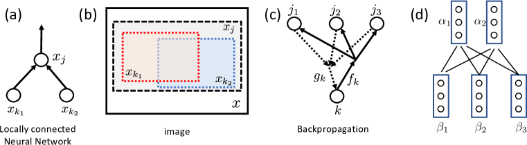
Figure 1: Problem Setting. (a) Locally connected network, (b) the receptive fields of each node. (c) notations used in backpropagation. (d) nodes with same receptive fields are grouped (Eqn. 56).

2.2 Locally Connected Network

Locally connected networks have extra structures, which leads to our reformulation. As shown in Fig. 1, each node $j$ only covers one part of the input images (i.e., receptive field). We use Greek letters $\{\alpha,\beta,\ldots,\omega\}$ to represent receptive fields. For a region $\alpha$, $x_{\alpha}$ is the content in that region. $j\in\alpha$ means node $j$ covers the region of $\alpha$ and $n_{\alpha}$ is the number of nodes that cover the same region (e.g., multi-channel case). The image content is $x_{\alpha(j)}$, abbreviated as $x_{j}$ if no ambiguity. The parent $j$’s receptive field covers its children’s. Finally, $\omega$ represents the entire image.

By definition, the activation $f_{j}$ of node $j$ is only dependent on the region $x_{j}$, rather than the entire image $x$. This means that $f_{j}(x)=f_{j}(x_{j})$ and $f_{j}(x_{j})=f^{\prime}_{j}(x_{j})\sum_{k}w_{jk}f_{k}(x_{k})$. However, the gradient $g_{j}$ is determined by the entire image $x$, and its label $y$, i.e., $g_{j}=g_{j}(x,y)$. Note that here we assume that the label $y$ is a deterministic (but unknown) function of $x$. Therefore, for gradient we just write $g_{j}=g_{j}(x)$.

2.3 Marginalized Gradient

Given the structure of locally connected network, the gradient $g_{j}$ has some nice structures. From Eqn. 2 we knows that $\Delta w_{jk}=\mathbb{E}_{x}\left[f_{k}(x)g_{j}(x)\right]=\mathbb{E}_{x_{k}}\left[f_{k}(x_{k})\mathbb{E}_{x_{-k}|x_{k}}\left[g_{j}(x)\right]\right]$. Define $x_{-k}=x\backslash x_{k}$ as the input image $x$ except for $x_{k}$. Then we can define the marginalized gradient:

$$g_{j}(x_{k})=\mathbb{E}_{x_{-k}|x_{k}}\left[g_{j}(x)\right]$$ (3)

as the marginalization (average) of $x_{-k}$, while keep $x_{k}$ fixed. With this notation, we can write $\Delta w_{jk}=\mathbb{E}_{x_{k}}\left[f_{k}(x_{k})g_{j}(x_{k})\right]$.

On the other hand, the gradient which back-propagates to a node $k$ can be written as

$$g_{k}(x)=f^{\prime}_{k}(x)\sum_{j\in\mathrm{pa}(k)}w_{jk}g_{j}(x)=f^{\prime}_{k}(x_{k})\sum_{j}w_{jk}g_{j}(x)$$ (4)

where $f^{\prime}_{k}$ is the derivative of activation function of node $k$ (for ReLU it is just a gating function). If we take expectation with respect to $x_{-k}|x_{k}$ on both side, we get

$$g_{k}(x_{k})=f^{\prime}_{k}(x_{k})g^{\mathrm{raw}}_{k}(x_{k})=f^{\prime}_{k}(x_{k})\sum_{j\in\mathrm{pa}(k)}w_{jk}g_{j}(x_{k})$$ (5)

Note that all marginalized gradients $g_{j}(x_{k})$ are independently computed by marginalizing with respect to all regions that are outside the receptive field $x_{k}$. Interestingly, there is a relationship between these gradients that respects the locality structure:

Theorem 1 (Recursive Property of marginalized gradient).

$g_{j}(x_{k})=\mathbb{E}_{x_{j,-k}|x_{k}}\left[g_{j}(x_{j})\right]$

This shows that the marginal gradient has recursive structure: we can first compute $g_{j}(x_{j})$ for top node $j$, then by marginalizing over the region within $x_{j}$ but outside $x_{k}$, we get its projection $g_{j}(x_{k})$ on child $k$, then by Eqn. 5 we collect all projections from all the parents of node $k$, to get $g_{k}(x_{k})$. This procedure can be repeated until we arrive at the leaf nodes.

3 Teacher-Student Setting

In order to analyze the behavior of neural network under backpropagation (BP), one needs to make assumptions about how the input $x$ is generated and how the label $y$ is related to the input $x$. Previous works assume Gaussian inputs and shallow networks, which yields analytic solution to gradient (Tian, 2017; Du et al., 2018), but might not align well with the practical data distribution.

3.1 The Summarization Ladder

We consider a multi-layered deterministic function as the teacher (not necessary a neural network). For each region $x_{\alpha}$, there is a latent discrete summarization variable $z_{\alpha}$ that captures the information of the input $x_{\alpha}$. Furthermore, we assume $z_{\alpha}=z_{\alpha}(x_{\alpha})=z_{\alpha}(\{z_{\beta}\}_{\beta\in\mathrm{ch}(\alpha)})$, i.e., the summarizaion only relies on the ones in the immediate lower layer. In particular, the top level summarization is the label of the image, $y=z_{\omega}$, where $\omega$ represents the region of the entire image. We call a particular assignment of $z_{\alpha}$, $z_{\alpha}=a$, an event. Finally, $m_{\alpha}$ is how many values $z_{\alpha}$ can take.

During training, all summarization functions $\mathcal{Z}=\{z_{\alpha}\}$ are unknown except for the label $y$.

3.2 Function Expansion on Summarization

Let’s consider the following quantity. For each neural node $j$, we want to compute the expected gradient given a particular factor $z_{\alpha}$, where $\alpha={\mathrm{rf}(j)}$ (the reception field of node $j$):

$$g_{j}(z_{\alpha})\equiv\mathbb{E}_{X_{j}|z_{\alpha}}\left[g_{j}(X_{j})\right]=\int g_{j}(x_{j})\mathbb{P}(x_{j}|z_{\alpha})\mathrm{d}x_{j}$$ (6)

And $\tilde{g}_{j}(z_{\alpha})=g_{j}(z_{\alpha})\mathbb{P}(z_{\alpha})$. Similarly, $f_{j}(z_{\alpha})=\mathbb{E}_{X_{j}|z_{\alpha}}\left[f_{j}(X_{j})\right]$ and $f^{\prime}_{j}(z_{\alpha})=\mathbb{E}_{X_{j}|z_{\alpha}}\left[f^{\prime}_{j}(X_{j})\right]$.

Note that $\mathbb{P}(x_{j}|z_{\alpha})$ is the frequency count of $x_{j}$ for $z_{\alpha}$. If $z_{\alpha}$ captures all information of $x_{j}$, then $\mathbb{P}(x_{j}|z_{\alpha})$ is a delta function. Throughout the paper, we use frequentist interpretation of probabilities.

Intuitively, if we have $g_{j}(z_{\alpha}=a)>0$ and $g_{j}(z_{\alpha}\neq a)<0$, then the node $j$ learns about the hidden event $z_{\alpha}=a$. For multi-class classification, the top level nodes (just below the softmax layer) already embrace such correlations (here $j$ is the class label):

$$g_{j}(y=j)>0,\quad g_{j}(y\neq j)<0,$$ (7)

where we know $z_{\omega}=y$ is the top level factor. A natural question now arises:

Does gradient descent automatically push $g_{j}(z_{\alpha})$ to be correlated with the factor $z_{\alpha}$?

If this is true, then gradient descent on deep models is essentially a weak-supervised approach that automatically learns the intermediate events at different levels. Giving a complete answer of this question is very difficult and is beyond the scope of this paper. Here, we aim to build a theoretical framework that enables such analysis. We start with the relationship between neighboring layers:

Theorem 2 (Reformulation).

Denote $\alpha={\mathrm{rf}(j)}$ and $\beta={\mathrm{rf}(k)}$. $k$ is a child of $j$. If the following conditions hold:

• Focus of knowledge. $\mathbb{P}(x_{k}|z_{\alpha},z_{\beta})=\mathbb{P}(x_{k}|z_{\beta})$.

• Broadness of knowledge. $\mathbb{P}(x_{j}|z_{\alpha},z_{\beta})=\mathbb{P}(x_{j}|z_{\alpha})$.

• Decorrelation. Given $z_{\beta}$, ($g_{k}^{\mathrm{raw}}(\cdot)$ and $f^{\prime}_{k}(\cdot)$) and ($f_{k}^{\mathrm{raw}}(\cdot)$ and $f^{\prime}_{k}(\cdot)$) are uncorrelated.

Then the following iterative equations hold:

$$f_{j}(z_{\alpha})\!=\!f_{j}^{\prime}(z_{\alpha})\!\sum_{k\in\mathrm{ch}(j)}w_{jk}\mathbb{E}_{z_{\beta}|z_{\alpha}}\left[f_{k}(z_{\beta})\right],\quad g_{k}(z_{\beta})\!=\!f_{k}^{\prime}(z_{\beta})\!\sum_{j\in\mathrm{pa}(k)}w_{jk}\mathbb{E}_{z_{\alpha}|z_{\beta}}\left[g_{j}(z_{\alpha})\right]$$ (8)

One key property of this formulation is that, it incorporates data distributions $\mathbb{P}(z_{\alpha},z_{\beta})$ into the gradient descent rules. This is important since running BP on different dataset is now formulated into the same framework with different probability, i.e., frequency counts of events. By studying which family of distribution leads to the desired property, we could understand BP better.

For completeness, we also need to define boundary conditions. In the lowest level $L$, we could treat each input pixel (or a group of pixels) as a single event. Therefore, $f_{k}(z_{\beta})=\mathbb{I}\left[k=z_{\beta}\right]$. On the top level, as we have discussed, Eqn. 7 applies and $g_{j}(z_{\beta})=a_{1}\mathbb{I}\left[j=z_{\beta}\right]-a_{2}\mathbb{I}\left[j\neq z_{\beta}\right]$.

The following theorem shows that the reformulation is exact if $z_{\alpha}$ has all information of the region.

Theorem 3.

If $\mathbb{P}(x_{j}|z_{\alpha})$ is a delta function for all $\alpha$, then all conditions in Thm. 2 hold.

In general, $\mathbb{P}(x_{j}|z_{\alpha})$ is a distribution encoding how much information gets lost if we only know the factor $z_{\alpha}$. When we climb up the ladder, we lose more and more information while keeping the critical part for the classification. This is consistent with empirical observations (Bau et al., 2017), in which the low-level features in DCNN are generic, and high-level features are more class-specific.

3.3 Matrix Formulation

Eqn. 8 can be hard to deal with. If we group the nodes with the same reception field at the same level together (Fig. 1(d)), we have the matrix form ($\circ$ is element-wise multiplication):

	Dimension	Description
$F_{\alpha}$, $\tilde{G}_{\alpha}$, $D_{\alpha}$	$m_{\alpha}$-by-$n_{\alpha}$	Activation $f_{j}(z_{\alpha})$, gradient $\tilde{g}_{j}(z_{\alpha})$ and gating prob $f^{\prime}_{j}(z_{\alpha})$ at group $\alpha$.
$W_{\beta\alpha}$	$n_{\beta}$-by-$n_{\alpha}$	Weight matrix that links group $\alpha$ and $\beta$
$P_{\alpha\beta}$	$m_{\alpha}$-by-$m_{\beta}$	Prob $\mathbb{P}(z_{\beta}|z_{\alpha})$ of events at group $\alpha$ and $\beta$

Table 1: Matrix Notation. See Eqn. 56.

Theorem 4 (Matrix Representation of Reformulation).

$$F_{\alpha}\!=\!D_{\alpha}\!\circ\!\sum_{\beta\in\mathrm{ch}(\alpha)}P_{\alpha\beta}F_{\beta}W_{\beta\alpha},\quad\tilde{G}_{\beta}\!=\!D_{\beta}\!\circ\!\sum_{\alpha\in\mathrm{pa}(\beta)}P_{\alpha\beta}^{T}\tilde{G}_{\alpha}W_{\beta\alpha}^{T},\quad\Delta W_{\beta\alpha}\!=\!(P_{\alpha\beta}F_{\beta})^{T}\tilde{G}_{\alpha}$$ (9)

See Tbl. 2 for the notation. For this dynamics, we want $F^{*}_{\omega}=I_{n_{\omega}}$, i.e., the top $n_{\omega}$ neurons faithfully represents the classification labels. Therefore, the top level gradient is $G_{\omega}=I_{n_{\omega}}-F_{\omega}$. On the other side, for each region $\beta$ at the bottom layer, we have $F_{\beta}=I_{n_{\beta}}$, i.e., the input contains all the preliminary factors. For all regions $\alpha$ in the top-most and bottom-most layers, we have $n_{\alpha}=m_{\alpha}$.

4 Batch Normalization under Reformulation

Our reformulation naturally incorporates empirical regularization technique like Batch Normalization (BN) (Ioffe & Szegedy, 2015).

Figure 2: Batch Normalization (BN) as a projection. (a) Three sublayers in BN (zero-mean, unit-variance, affine). (b) The gradient $\mathbf{g}_{\mathbf{f}}$ that is propagated down is a projection of input gradient $\mathbf{g}$ onto the orthogonal complementary space spanned by $\{\mathbf{f},\mathbf{1}\}$.

4.1 Batch Normalization as a Projection

We start with a novel finding of Batch Norm: the back-propagated gradient through Batch Norm layer at a node $j$ is a projection onto the orthogonal complementary subspace spanned by all one vectors and the current activations of node $j$.

Denote pre-batchnorm activations as $f^{(i)}=f_{j}(x_{i})$ ($i=1\ldots N$). In Batch Norm, $f^{(i)}$ is whitened to be $\tilde{f}^{(i)}$, then linearly transformed to yield the output $\bar{f}^{(i)}$:

$$\hat{f}^{(i)}=f^{(i)}-\mu,\quad\tilde{f}^{(i)}=\hat{f}^{(i)}/\sigma,\quad\bar{f}^{(i)}=c_{1}\tilde{f}^{(i)}+c_{0}$$ (10)

where $\mu=\frac{1}{N}\sum_{i}f^{(i)}$ and $\sigma^{2}=\frac{1}{N}\sum_{i}(f^{(i)}-\mu)^{2}$ and $c_{1}$, $c_{0}$ are learnable parameters.

The original Batch Norm paper derives complicated and unintuitive weight update rules. With vector notation, the update has a compact form with clear geometric meaning.

Theorem 5 (Backpropagation of Batch Norm).

For a top-down gradient $\mathbf{g}$, BN layer gives the following gradient update ($P^{\perp}_{\mathbf{f},\mathbf{1}}$ is the orthogonal complementary projection of subspace $\{\mathbf{f},\mathbf{1}\}$):

$$\mathbf{g}_{\mathbf{f}}=J^{BN}(\mathbf{f})\mathbf{g}=\frac{c_{1}}{\sigma}P^{\perp}_{\mathbf{f},\mathbf{1}}\mathbf{g},\quad\mathbf{g}_{\mathbf{c}}=S(\mathbf{f}{})^{T}\mathbf{g}$$ (11)

Intuitively, the back-propagated gradient $J^{BN}(\mathbf{f})\mathbf{g}$ is zero-mean and perpendicular to the input activation $\mathbf{f}$ of BN layer, as illustrated in Fig. 2. Unlike (Kohler et al., 2018) that analyzes BN in an approximate manner, in Thm. 5 we do not impose any assumptions.

4.2 Batch Norm under the reformulation

The analysis of Batch Norm is compatible with the reformulation and we arrive at similar backpropagation rule, by noticing that $\mathbb{E}_{x}\left[f_{j}(x)\right]=\mathbb{E}_{z_{\alpha}}\left[f_{j}(z_{\alpha})\right]$:

$$\mu=\mathbb{E}_{z_{\alpha}}\left[f_{j}\right],\quad\sigma^{2}=\mathbb{E}_{z_{\alpha}}\left[(f_{j}(z_{\alpha})-\mu)^{2}\right],\quad J^{BN}(\mathbf{f}{})=\frac{c_{1}}{\sigma}P^{\perp}_{\mathbf{f},\mathbf{1}}$$ (12)

Note that we still have the projection property, but under the new inner product $\langle f_{j},g_{j}\rangle_{z_{\alpha}}=\mathbb{E}_{z_{\alpha}}\left[f_{j}(z_{\alpha})g_{j}(z_{\alpha})\right]$ and norm $\|f\|_{z_{\alpha}}=\langle f,f\rangle_{z_{\alpha}}^{1/2}$.

5 Example applications of proposed theoretical framework

With the help of the theoretical framework, we now can analyze interesting structures of gradient descent in deep models, when the data distribution $\mathbb{P}(z_{\alpha},z_{\beta})$ satisfies specific conditions. Here we give two concrete examples: the role played by nonlinearity and in which condition disentangled representation can be achieved. Besides, from the theoretical framework, we also give general comments on multiple issues (e.g., overfitting, GD versus SGD) in deep learning.

5.1 Nonlinear versus linear

In the formulation, $m_{\alpha}$ is the number of possible events within a region $\alpha$, which is often exponential with respect to the size $\mathrm{sz}(\alpha)$ of the region. The following analysis shows that a linear model cannot handle it, even with exponential number of nodes $n_{\alpha}$, while a nonlinear one with ReLU can.

Definition 1 (Convex Hull of a Set).

We define the convex hull $\mathrm{Conv}(P)$ of $m$ points $P\subset\mathbb{R}^{n}$ to be $\mathrm{Conv}(P)=\left\{P\mathbf{a},\mathbf{a}\in\boldsymbol{\Delta}^{n-1}\right\}$, where $\boldsymbol{\Delta}^{n-1}=\left\{\mathbf{a}\in\mathbb{R}^{n},a_{i}\geq 0,\sum_{i}a_{i}=1\right\}$. A row $p_{j}$ is called vertex if $p_{j}\notin\mathrm{Conv}(P\backslash p_{j})$.

Definition 2.

A matrix $P$ of size $m$-by-$n$ is called $k$-vert, or $\mathrm{vert}(P)=k\leq m$, if its $k$ rows are vertices of the convex hull generated by its rows. $P$ is called all-vert if $k=m$.

Theorem 6 (Expressibility of ReLU Nonlinearity).

Assuming $m_{\alpha}=n_{\alpha}=\mathcal{O}(\exp(\mathrm{sz}(\alpha)))$, where $\mathrm{sz}(\alpha)$ is the size of receptive field of $\alpha$. If each $P_{\alpha\beta}$ is all-vert, then: ($\omega$ is top-level receptive field)

$$\min_{W}Loss_{\mathrm{ReLU}}(W)=0,\quad\min_{W}Loss_{\mathrm{Linear}}(W)=\mathcal{O}(\exp(\mathrm{sz}(\omega)))$$ (13)

Note that here $Loss(W)\equiv\|F_{\omega}-I\|^{2}_{F}$. This shows the power of nonlinearity, which guarantees full rank of output, even if the matrices involved in the multiplication are low-rank. The following theorem shows that for intermediate layers whose input is not identity, the all-vert property remains.

Theorem 7.

(1) If $F$ is full row rank, then $\mathrm{vert}(PF)=\mathrm{vert}(P)$. (2) $PF$ is all-vert iff $P$ is all-vert.

This means that if all $P_{\alpha\beta}$ are all-vert and its input $F_{\beta}$ is full-rank, then with the same construction of Thm. 6, $F_{\alpha}$ can be made identity. In particular, if we sample $W$ randomly, then with probability $1$, all $F_{\beta}$ are full-rank, in particular the top-level input $F_{1}$. Therefore, using top-level $W_{1}$ alone would be sufficient to yield zero generalization error, as shown in the previous works that random projection could work well.

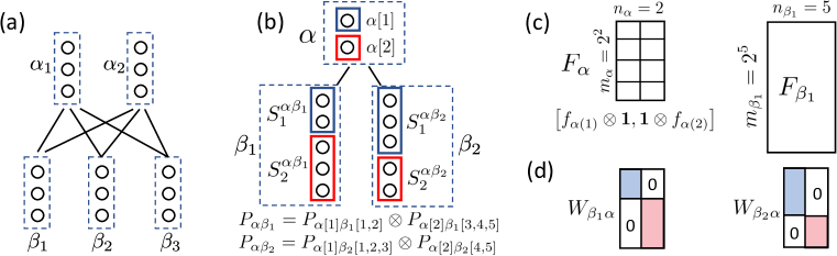
Figure 3: disentangled representation. (a) Nodes are grouped according to regions. (b) An example of one parent region $\alpha$ ($2$ nodes) and two child regions $\beta_{1}$ and $\beta_{2}$ ($5$ nodes each). We assume factorization property of data distribution $P$. (c) disentangled activations, (d) Separable weights.

5.2 disentangled Representation

The analysis in Sec. 5.1 assumes that $n_{\alpha}=m_{\alpha}$, which means that we have sufficient nodes, one neuron for one event, to convey the information forward to the classification level. In practice, this is never the case. When $n_{\alpha}\ll m_{\alpha}=\mathcal{O}(\exp(\mathrm{sz}(\alpha)))$ and the network needs to represent the information in a proper way so that it can be sent to the top level. Ideally, if the factor $z_{\alpha}$ can be written down as a list of binary factors: $z_{\alpha}=\left[z_{\alpha[1]},z_{\alpha[2]},\ldots,z_{\alpha[j]}\right]$, the output of a node $j$ could represent $z_{\alpha[j]}$, so that all $m_{\alpha}$ events can be represented concisely with $n_{\alpha}$ nodes.

To come up with a complete theory for disentangled representation in deep nonlinear network is far from trivial and beyond the scope of this paper. In the following, we make an initial attempt by constructing factorizable $P_{\alpha\beta}$ so that disentangled representation is possible in the forward pass. First we need to formally define what is disentangled representation:

Definition 3.

The activation $F_{\alpha}$ is disentangled, if its $j$-th column $F_{\alpha,:j}=\mathbf{1}\otimes\ldots\!\otimes\!\mathbf{f}_{\alpha[j]}\!\otimes\!\ldots\!\otimes\!\mathbf{1}$, where each $\mathbf{f}_{\alpha[j]}$ and $\mathbf{1}$ is a $2$-by-$1$ vector.

Definition 4.

The gradient $\tilde{G}_{\alpha}$ is disentangled, if its $j$-th column $\tilde{G}_{\alpha,:j}=\mathbf{p}_{\alpha[1]}\otimes\ldots\!\otimes\!\tilde{\mathbf{g}}_{\alpha[j]}\!\otimes\!\ldots\!\otimes\!\mathbf{p}_{\alpha[n_{\alpha}]}$, where $\mathbf{p}_{\alpha[j]}=\left[\mathbb{P}(\alpha[j]=0),\mathbb{P}(\alpha[j]=1)\right]^{T}$ and $\tilde{\mathbf{g}}_{\alpha[j]}$ is a $2$-by-$1$ vector.

Intuitively, this means that each node $j$ represents the binary factor $z_{\alpha}[j]$. A follow-up question is whether such disentangled properties carries over layers in the forward pass. It turns out that the disentangled structure carries if the data distribution and weights have compatible structures:

Definition 5.

The weights $W_{\beta\alpha}$ is separable with respect to a disjoint set $\{S^{\alpha\beta}_{i}\}$, if $W_{\beta\alpha}=\mathrm{diag}\left(W_{\beta\alpha}[S^{\alpha\beta}_{1},1],W_{\beta\alpha}[S^{\alpha\beta}_{2},2],\ldots,W_{\beta\alpha}[S^{\alpha\beta}_{n_{\alpha}},n_{\alpha}]\right)$.

Theorem 8 (Disentangled Forward).

If for each $\beta\in\mathrm{ch}(\alpha)$, $P_{\alpha\beta}$ can be written as a tensor product $P_{\alpha\beta}=\bigotimes_{i}P_{\alpha[i]\beta[S^{\alpha\beta}_{i}]}$ where $\{S^{\alpha\beta}_{i}\}$ are $\alpha\beta$-dependent disjointed set, $W_{\beta\alpha}$ is separable with respect to $\{S^{\alpha\beta}_{i}\}$, $F_{\beta}$ is disentangled, then $F_{\alpha}$ is also disentangled (with/without ReLU /Batch Norm).

If the bottom activations are disentangled, by induction, all activations will be disentangled. The next question is whether gradient descent preserves such a structure. The answer is also conditionally yes:

Theorem 9 (Separable Weight Update).

If $P_{\alpha\beta}=\bigotimes_{i}P_{\alpha[i]\beta[S_{i}]}$, $F_{\beta}$ and $\tilde{G}_{\alpha}$ are both disentangled, $\mathbf{1}^{T}\tilde{G}_{\alpha}=\mathbf{0}$, then the gradient update $\Delta W_{\beta\alpha}$ is separable with respect to $\{S_{i}\}$.

Therefore, with disentangled $F_{\beta}$ and $\tilde{G}_{\alpha}$ and centered gradient $\mathbf{1}^{T}\tilde{G}_{\alpha}=\mathbf{0}$, the separable structure is conserved over gradient descent, given the initial $W^{(0)}_{\beta\alpha}$ is separable. Note that centered gradient is guaranteed if we insert Batch Norm (Eqn. 12) after linear layers. And the activation $F$ remains disentangled if the weights are separable.

The hard part is whether $\tilde{G}_{\beta}$ remains disentangled during backpropagation, if $\{\tilde{G}_{\alpha}\}_{\alpha\in\mathrm{pa}(\beta)}$ are all disentangled. If so, then the disentangled representation is self-sustainable under gradient descent. This is a non-trivial problem and generally requires structures of data distribution. We put some discussion in the Appendix and leave this topic for future work.

5.3 Explanation of common behaviors in Deep Learning

In the proposed formulation, the input $x$ in Eqn. 8 is integrated out, and the data distribution is now encoded into the probabilistic distribution $\mathbb{P}(z_{\alpha},z_{\beta})$, and their marginals. A change of such distribution means the input distribution has changed. For the first time, we can now analyze many practical factors and behaviors in the DL training that is traditionally not included in the formulation.

Over-fitting. Given finite number of training samples, there is always error in estimated factor-factor distribution $\tilde{\mathbb{P}}(z_{\alpha},z_{\beta})$ and factor-observation distribution $\tilde{\mathbb{P}}(x_{\alpha}|z_{\alpha})$. In some cases, a slight change of distribution would drastically change the optimal weights for prediction, which is overfitting.

Here is one example. Suppose there are two different kinds of events at two disjoint reception fields: $z_{\alpha}$ and $z_{\gamma}$. The class label is $z_{\omega}$, which equals $z_{\alpha}$ but is not related to $z_{\gamma}$. Therefore, we have:

$$\tilde{\mathbb{P}}(z_{\omega}=1|z_{\alpha}=1)=1,\quad\tilde{\mathbb{P}}(z_{\omega}=1|z_{\alpha}=0)=0$$ (14)

Although $z_{\gamma}$ is unrelated to the class label $z_{\omega}$, with finite samples $z_{\gamma}$ could show spurious correlation:

$$\tilde{\mathbb{P}}(z_{\omega}=1|z_{\gamma}=1)=0.5+\epsilon,\quad\tilde{\mathbb{P}}(z_{\omega}=1|z_{\gamma}=0)=0.5-\epsilon$$ (15)

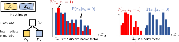
Figure 4: Overfitting Example

On the other hand, as shown in Fig. 4, $\mathbb{P}(x_{\alpha}|z_{\alpha})$ contains a lot of detailed structures and is almost impossible to separate in the finite sample case, while $\mathbb{P}(x_{\gamma}|z_{\gamma})$ could be well separated for $z_{\gamma}=0/1$. Therefore, for node $j$ with ${\mathrm{rf}(j)}=\alpha$, $f_{j}(z_{\alpha})\approx\mathrm{constant}$ (input almost indistinguishable):

$$\Delta w_{j}=\mathbb{E}_{z_{\alpha}}\left[f_{j}(z_{\alpha})g_{0}(z_{\alpha})\right]\approx 0$$ (16)

where $g_{0}(z_{\alpha})=\mathbb{E}_{z_{\omega}|z_{\alpha}}\left[g_{0}(z_{\omega})\right]=\left\{\begin{array}[]{cc}1&z_{\alpha}=1\\ -1&z_{\alpha}=0\end{array}\right.$, which is a strong gradient signal backpropagated from the top softmax level, since $z_{\alpha}$ is strongly correlated with $z_{\omega}$. For node $k$ with ${\mathrm{rf}(k)}=\gamma$, an easy separation of the input (e.g., random initialization) yields distinctive $f_{k}(z_{\gamma})$. Therefore,

$$\Delta w_{k}=\mathbb{E}_{z_{\gamma}}\left[f_{j}(z_{\gamma})g_{0}(z_{\gamma})\right]>0$$ (17)

where $g_{0}(z_{\gamma})=\mathbb{E}_{z_{\omega}|z_{\gamma}}\left[g_{0}(z_{\omega})\right]=\left\{\begin{array}[]{cc}2\epsilon&z_{\gamma}=1\\ -2\epsilon&z_{\gamma}=0\end{array}\right.$, a weak signal because of $z_{\gamma}$ is (almost) unrelated to the label. Therefore, we see that the weight $w_{j}$ that links to meaningful receptive field $z_{\alpha}$ does not receive strong gradient, while the weight $w_{k}$ that links to irrelevant (but spurious) receptive field $z_{\gamma}$ receives strong gradient. This will lead to overfitting.

With more data, over-fitting is alleviated since (1) $\tilde{\mathbb{P}}(z_{\omega}|z_{\gamma})$ becomes more accurate and $\epsilon\rightarrow 0$; (2) $\tilde{\mathbb{P}}(x_{\alpha}|z_{\alpha})$ starts to show statistical difference for $z_{\alpha}=0/1$ and thus $f_{j}(z_{\alpha})$ shows distinctiveness.

Note that there exists a second explanation: we could argue that $z_{\gamma}$ is a true but weak factor that contributes to the label, while $z_{\alpha}$ is a fictitious discriminative factor, since the appearance difference between $z_{\alpha}=0$ and $z_{\alpha}=1$ (i.e., $\tilde{\mathbb{P}}(x_{\alpha}|z_{\alpha})$ for $\alpha=0/1$) could be purely due to noise and thus should be neglected. With finite number of samples, these two cases are essentially indistinguishable. Models with different induction bias might prefer one to the other, yielding drastically different generalization error. For neural network, SGD prefers the second explanation but if under the pressure of training, it may also explore the first one by pushing gradient down to distinguish subtle difference in the input. This may explain why the same neural networks can fit random-labeled data, and generalize well for real data (Zhang et al., 2016).

Gradient Descent: Stochastic or not? Previous works (Keskar et al., 2017) show that empirically stochastic gradient decent (SGD) with small batch size tends to converge to “flat” minima and offers better generalizable solution than those uses larger batches to compute the gradient.

From our framework, SGD update with small batch size is equivalent to using a perturbed/noisy version of $\mathbb{P}(z_{\alpha},z_{\beta})$ at each iteration. Such an approach naturally reduces aforementioned over-fitting issues, which is due to hyper-sensitivity of data distribution and makes the final weight solution invariant to changes in $\mathbb{P}(z_{\alpha},z_{\beta})$, yielding a “flat” solution.

6 Conclusion and future work

In this paper, we propose a novel theoretical framework for deep (multi-layered) nonlinear network with ReLU activation and local receptive fields. The framework utilizes the specific structure of neural networks, and formulates input data distributions explicitly. Compared to modeling deep models as non-convex problems, our framework reveals more structures of the network; compared to recent works that also take data distribution into considerations, our theoretical framework can model deep networks without imposing idealistic analytic distribution of data like Gaussian inputs or independent activations. Besides, we also analyze regularization techniques like Batch Norm, depicts its underlying geometrical intuition, and shows that BN is compatible with our framework.

Using this novel framework, we have made an initial attempt to analyze many important and practical issues in deep models, and provides a novel perspective on overfitting, generalization, disentangled representation, etc. We emphasize that in this work, we barely touch the surface of these core issues in deep learning. As a future work, we aim to explore them in a deeper and more thorough manner, by using the powerful theoretical framework proposed in this paper.

7 Appendix

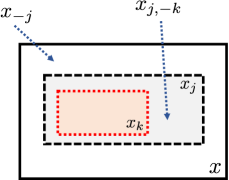
Figure 5: Notation used in Thm. 1.

7.1 Hierarchical Conditioning

Theorem 1 (Recursive Property of marginalized gradient).

$$g_{j}(x_{k})=\mathbb{E}_{x_{j,-k}|x_{k}}\left[g_{j}(x_{j})\right]$$ (18)

Proof.

We have:

$$g_{j}(x_{k}) =\mathbb{E}_{x_{-k}|x_{k}}\left[g_{j}(x)\right]$$

$$=\mathbb{E}_{x_{-j},x_{j,-k}|x_{k}}\left[g_{j}(x)\right]$$

$$=\mathbb{E}_{x_{-j}|x_{j,-k},x_{k}}\left[\mathbb{E}_{x_{j,-k}|x_{k}}\left[g_{j}(x)\right]\right]$$

$$=\mathbb{E}_{x_{-j}|x_{j}}\left[\mathbb{E}_{x_{j,-k}|x_{k}}\left[g_{j}(x)\right]\right]$$

$$=\mathbb{E}_{x_{j,-k}|x_{k}}\left[\mathbb{E}_{x_{-j}|x_{j}}\left[g_{j}(x)\right]\right]$$

$$=\mathbb{E}_{x_{j,-k}|x_{k}}\left[g_{j}(x_{j})\right]$$

∎

7.2 Network theorem

Theorem 2 (Reformulation).

Denote $\alpha={\mathrm{rf}(j)}$ and $\beta={\mathrm{rf}(k)}$. $k$ is a child of $j$. If the following two conditions hold:

• Focus of knowledge. $\mathbb{P}(x_{k}|z_{\alpha},z_{\beta})=\mathbb{P}(x_{k}|z_{\beta})$.

• Broadness of knowledge. $\mathbb{P}(x_{j}|z_{\alpha},z_{\beta})=\mathbb{P}(x_{j}|z_{\alpha})$.

• Decorrelation. Given $z_{\beta}$, ($g_{k}^{\mathrm{raw}}(\cdot)$ and $f^{\prime}_{k}(\cdot)$) and ($f_{k}^{\mathrm{raw}}(\cdot)$ and $f^{\prime}_{k}(\cdot)$) are uncorrelated

Then the following two conditions holds:

$$f_{j}(z_{\alpha}) =f_{j}^{\prime}(z_{\alpha})\sum_{k\in\mathrm{ch}(j)}w_{jk}\mathbb{E}_{z_{\beta}|z_{\alpha}}\left[f_{k}(z_{\beta})\right]$$ (19a)

$$g_{k}(z_{\beta}) =f_{k}^{\prime}(z_{\beta})\sum_{j\in\mathrm{pa}(k)}w_{jk}\mathbb{E}_{z_{\alpha}|z_{\beta}}\left[g_{j}(z_{\alpha})\right]$$ (19b)

Proof.

For Eqn. 19a, we have:

$$f_{j}^{\mathrm{raw}}(z_{\alpha}) =\int f_{j}^{\mathrm{raw}}(x)\mathbb{P}(x|z_{\alpha})\mathrm{d}x$$ (20)

$$=\int f_{j}^{\mathrm{raw}}(x_{j})\mathbb{P}(x_{j}|z_{\alpha})\mathrm{d}x_{j}$$ (21)

$$=\int\left(\sum_{k\in\mathrm{ch}(j)}w_{jk}f_{k}(x_{k})\right)\mathbb{P}(x_{j}|z_{\alpha})\mathrm{d}x_{j}$$ (22)

And for each of the entry, we have:

$$\int f_{k}(x_{k})\mathbb{P}(x_{j}|z_{\alpha})\mathrm{d}x_{j} =\int f_{k}(x_{k})\mathbb{P}(x_{k}|z_{\alpha})\mathrm{d}x_{k}$$ (23)

For $\mathbb{P}(x_{k}|z_{\alpha})$, using focus of knowledge, we have:

$$\mathbb{P}(x_{k}|z_{\alpha}) =\sum_{z_{\beta}}\mathbb{P}(x_{k},z_{\beta}|z_{\alpha})$$ (24)

$$=\sum_{z_{\beta}}\mathbb{P}(x_{k}|z_{\beta},z_{\alpha})\mathbb{P}(z_{\beta}|z_{\alpha})$$ (25)

$$=\sum_{z_{\beta}}\mathbb{P}(x_{k}|z_{\beta})\mathbb{P}(z_{\beta}|z_{\alpha})$$ (26)

Therefore, following Eqn. 23, we have:

$$\int f_{k}(x_{k})\mathbb{P}(x_{k}|z_{\alpha})\mathrm{d}x_{k} =\int f_{k}(x_{k})\sum_{z_{\beta}}\mathbb{P}(x_{k}|z_{\beta})\mathbb{P}(z_{\beta}|z_{\alpha})\mathrm{d}x_{k}$$ (27)

$$=\sum_{z_{\beta}}\left(\int f_{k}(x_{k})\mathbb{P}(x_{k}|z_{\beta})\mathrm{d}x_{k}\right)\mathbb{P}(z_{\beta}|z_{\alpha})$$ (28)

$$=\sum_{z_{\beta}}f_{k}(z_{\beta})\mathbb{P}(z_{\beta}|z_{\alpha})$$ (29)

$$=\mathbb{E}_{z_{\beta}|z_{\alpha}}\left[f_{k}(z_{\beta})\right]$$ (30)

Putting it back to Eqn. 22 and we have:

$$f_{j}^{\mathrm{raw}}(z_{\alpha})=\sum_{k\in\mathrm{ch}(j)}w_{jk}\mathbb{E}_{z_{\beta}|z_{\alpha}}\left[f_{k}(z_{\beta})\right]$$ (31)

For Eqn. 19b, similarly we have:

$$g^{\mathrm{raw}}_{k}(z_{\beta}) =\int g_{k}^{\mathrm{raw}}(x)\mathbb{P}(x|z_{\beta})\mathrm{d}x$$ (32)

$$=\int\sum_{j\in\mathrm{pa}(k)}w_{jk}g_{j}(x)\mathbb{P}(x|z_{\beta})\mathrm{d}x$$ (33)

Notice that we have:

$$\mathbb{P}(x|z_{\beta})=\mathbb{P}(x_{j}|z_{\beta})\mathbb{P}(x_{-j}|x_{j},z_{\beta})=\mathbb{P}(x_{j}|z_{\beta})\mathbb{P}(x_{-j}|x_{j})$$ (34)

since $x_{j}$ covers $x_{k}$ which determines $z_{\beta}$. Therefore, for each item we have:

$$\int g_{j}(x)\mathbb{P}(x|z_{\beta})\mathrm{d}x =\int g_{j}(x)\mathbb{P}(x_{j}|z_{\beta})\mathbb{P}(x_{-j}|x_{j})\mathrm{d}x$$ (35)

$$=\int\left(\int g_{j}(x)\mathbb{P}(x_{-j}|x_{j})\mathrm{d}x_{-j}\right)\mathbb{P}(x_{j}|z_{\beta})\mathrm{d}x_{j}$$ (36)

$$=\int g_{j}(x_{j})\mathbb{P}(x_{j}|z_{\beta})\mathrm{d}x_{j}$$ (37)

Then we use the broadness of knowledge:

$$\mathbb{P}(x_{j}|z_{\beta}) =\sum_{z_{\alpha}}\mathbb{P}(x_{j},z_{\alpha}|z_{\beta})$$ (38)

$$=\sum_{z_{\alpha}}\mathbb{P}(x_{j}|z_{\alpha},z_{\beta})\mathbb{P}(z_{\alpha}|z_{\beta})$$ (39)

$$=\sum_{z_{\alpha}}\mathbb{P}(x_{j}|z_{\alpha})\mathbb{P}(z_{\alpha}|z_{\beta})$$ (40)

Following Eqn. 37, we now have:

$$\int g_{j}(x)\mathbb{P}(x|z_{\beta})\mathrm{d}x =\int g_{j}(x_{j})\sum_{z_{\alpha}}\mathbb{P}(x_{j}|z_{\alpha})\mathbb{P}(z_{\alpha}|z_{\beta})\mathrm{d}x_{j}$$ (41)

$$=\sum_{z_{\alpha}}\left(\int g_{j}(x_{j})\mathbb{P}(x_{j}|z_{\alpha})\mathrm{d}x_{j}\right)\mathbb{P}(z_{\alpha}|z_{\beta})$$ (42)

$$=\sum_{z_{\alpha}}g_{j}(z_{\alpha})\mathbb{P}(z_{\alpha}|z_{\beta})$$ (43)

$$=\mathbb{E}_{z_{\alpha}|z_{\beta}}\left[g_{j}(z_{\alpha})\right]$$ (44)

Putting it back to Eqn. 33 and we have:

$$g^{\mathrm{raw}}_{k}(z_{\beta})=\sum_{j\in\mathrm{pa}(k)}w_{jk}\mathbb{E}_{z_{\alpha}|z_{\beta}}\left[g_{j}(z_{\alpha})\right]$$ (45)

Using Eqn. 5:

$$g_{k}(z_{\beta}) =\int g_{k}(x_{k})\mathbb{P}(x_{k}|z_{\beta})\mathrm{d}x_{k}$$ (46)

$$=\int f_{k}^{\prime}(x_{k})g^{\mathrm{raw}}_{k}(x_{k})\mathbb{P}(x_{k}|z_{\beta})\mathrm{d}x_{k}$$ (47)

$$=\mathbb{E}_{X_{k}|z_{\beta}}\left[f^{\prime}_{k}(X_{k})g_{k}^{\mathrm{raw}}(X_{k})\right]$$ (48)

The un-correlation between $g_{k}^{\mathrm{raw}}(\cdot)$ and $f^{\prime}_{k}(\cdot)$ means that

$$\mathbb{E}_{X_{k}|z_{\beta}}\left[f^{\prime}_{k}g_{k}^{\mathrm{raw}}\right] =\mathbb{E}_{X_{k}|z_{\beta}}\left[f^{\prime}_{k}\right]\cdot\mathbb{E}_{X_{k}|z_{\beta}}\left[g_{k}^{\mathrm{raw}}\right]$$ (49)

Similarly for $f_{j}(z_{\alpha})$. ∎

7.3 Exactness of reformulation

Theorem 3.

If $\mathbb{P}(x_{j}|z_{\alpha})$ is a delta function for all $\alpha$, then the conditions of Thm. 2 hold and the reformulation becomes exact.

Proof.

The fact that $\mathbb{P}(x_{j}|z_{\alpha})$ is a delta function means that there exists a function $\phi_{j}$ so that:

$$\mathbb{P}(x_{j}|z_{\alpha})=\delta(x_{j}-\phi_{j}(z_{\alpha}))$$ (50)

That is, $z_{\alpha}$ contains all information of $x_{j}$ (or $x_{\alpha}$). Therefore,

• Broadness of knowledge. $z_{\alpha}$ contains strictly more information than $z_{\beta}$ for $\beta\in\mathrm{ch}(\alpha)$, therefore $\mathbb{P}(x_{j}|z_{\alpha},z_{\beta})=\mathbb{P}(x_{j}|z_{\alpha})$.

• Focus of knowledge. $z_{\beta}$ captures all information of $z_{k}$, so $\mathbb{P}(x_{k}|z_{\alpha},z_{\beta})=\mathbb{P}(x_{k}|z_{\beta})$.

• Decorrelation. For any $h_{1}(x_{j})$ and $h_{2}(x_{j})$ we have

  $$\mathbb{E}_{X_{j}|z_{\alpha}}\left[h_{1}h_{2}\right] =\int h_{1}(x_{j})h_{2}(x_{j})\mathbb{P}(x_{j}|z_{\alpha})\mathrm{d}x_{j}$$ (51)

  $$=\int h_{1}(x_{j})h_{2}(x_{j})\delta(x_{j}-\phi_{j}(z_{\alpha}))\mathrm{d}x_{j}$$ (52)

  $$=h_{1}(\phi_{j}(z_{\alpha}))h_{2}(\phi_{j}(z_{\alpha}))$$ (53)

  $$=\int h_{1}(x_{j})\mathbb{P}(x_{j}|z_{\alpha})\mathrm{d}x_{j}\int h_{2}(x_{j})\mathbb{P}(x_{j}|z_{\alpha})\mathrm{d}x_{j}$$ (54)

  $$=\mathbb{E}_{X_{j}|z_{\alpha}}\left[h_{1}\right]\mathbb{E}_{X_{j}|z_{\alpha}}\left[h_{2}\right]$$ (55)

∎

7.4 Matrix form

Theorem 4 (Matrix Representation of Reformulation).

$$F_{\alpha}\!=\!D_{\alpha}\!\circ\!\sum_{\beta\in\mathrm{ch}(\alpha)}P_{\alpha\beta}F_{\beta}W_{\beta\alpha},\quad\tilde{G}_{\beta}\!=\!D_{\beta}\!\circ\!\sum_{\alpha\in\mathrm{pa}(\beta)}P_{\alpha\beta}^{T}\tilde{G}_{\alpha}W_{\beta\alpha}^{T},\quad\Delta W_{\beta\alpha}\!=\!(P_{\alpha\beta}F_{\beta})^{T}\tilde{G}_{\alpha}$$ (56)

Proof.

We first consider one certain group $\alpha$ and $\beta$, which uses $x_{\alpha}$ and $x_{\beta}$ as the receptive field. For this pair, we can write Eqn. 19 in the following matrix form:

$$F^{\mathrm{raw}}_{\alpha} =P_{\alpha\beta}F_{\beta}W_{\beta\alpha}$$ (57a)

$$F_{\alpha} =F^{\mathrm{raw}}_{\alpha}\circ D_{\alpha}$$ (57b)

$$G^{\mathrm{raw}}_{\beta} =\left(P^{b}_{\alpha\beta}\right)^{T}G_{\beta}W_{\beta\alpha}^{T}$$ (57c)

$$G_{\beta} =G^{\mathrm{raw}}_{\beta}\circ D_{\beta}$$ (57d)

	Dimension	Description
$F_{\alpha}$, $D_{\alpha}$	$m_{\alpha}$-by-$n_{\alpha}$	Activation $f_{j}(z_{\alpha})$ and gating prob $f^{\prime}_{j}(z_{\alpha})$ in group $\alpha$.
$G_{\alpha}$, $\tilde{G}_{\alpha}$	$m_{\alpha}$-by-$n_{\alpha}$	Gradient $g_{j}(z_{\alpha})$ and unnormalized gradient $\tilde{g}_{j}(z_{\alpha})$ in group $\alpha$.
$W_{\beta\alpha}$	$n_{\beta}$-by-$n_{\alpha}$	Weight matrix that links group $\beta$ and $\alpha$.
$P_{\alpha\beta}$, $P^{b}_{\alpha\beta}$	$m_{\alpha}$-by-$m_{\beta}$	Prob $\mathbb{P}(z_{\beta}|z_{\alpha})$, $\mathbb{P}(z_{\alpha}|z_{\beta})$ of events between group $\beta$ and $\alpha$.
$\Lambda_{\alpha}$	$m_{\alpha}$-by-$m_{\alpha}$	Diagonal matrix encoding prior prob $\mathbb{P}(z_{\alpha})$.

Table 2: Matrix Notation. See Eqn. 56.

Using $\Lambda_{\beta}(P^{b}_{\alpha\beta})^{T}=P_{\alpha\beta}^{T}\Lambda_{\alpha}$ and $\tilde{G}_{\alpha}=\Lambda_{\alpha}G_{\alpha}$, we could simplify Eqn. 57 as follows:

$$F_{\alpha} =P_{\alpha\beta}F_{\beta}W_{\beta\alpha}\circ D_{\alpha}$$ (58a)

$$\tilde{G}_{\beta} =\left(P_{\alpha\beta}\right)^{T}\tilde{G}_{\beta}W_{\beta\alpha}^{T}\circ D_{\beta}$$ (58b)

Therefore, using the fact that $\sum_{j\in\mathrm{pa}(k)}=\sum_{\alpha\in\mathrm{pa}(\beta)}\sum_{j\in\alpha}$ (where $\beta={\mathrm{rf}(k)}$) and $\sum_{k\in\mathrm{ch}(j)}=\sum_{\beta\in\mathrm{ch}(\alpha)}\sum_{k\in\beta}$ (where $\alpha={\mathrm{rf}(j)}$), and group all nodes that share the receptive field together, we have:

$$F_{\alpha} =D_{\alpha}\circ\sum_{\beta\in\mathrm{ch}(\alpha)}P_{\alpha\beta}F_{\beta}W_{\beta\alpha}$$ (59a)

$$\tilde{G}_{\beta} =D_{\beta}\circ\sum_{\alpha\in\mathrm{pa}(\beta)}P_{\alpha\beta}^{T}\tilde{G}_{\alpha}W_{\beta\alpha}^{T}$$ (59b)

For the gradient update rule, from Eqn. 2 notice that:

$$\Delta w_{jk} =\mathbb{E}_{x}\left[f_{k}(x)g_{j}(x)\right]$$ (60)

$$=\int f_{k}(x)g_{j}(x)\mathbb{P}(x)\mathrm{d}x$$ (61)

$$=\int f_{k}(x)g_{j}(x)\sum_{z_{\alpha}}\mathbb{P}(x|z_{\alpha})\mathbb{P}(z_{\alpha})\mathrm{d}x$$ (62)

$$=\sum_{z_{\alpha}}\int f_{k}(x)g_{j}(x)\mathbb{P}(x|z_{\alpha})\mathbb{P}(z_{\alpha})\mathrm{d}x$$ (63)

We assume decorrelation so we have:

$$\Delta w_{jk} =\sum_{z_{\alpha}}\mathbb{E}_{X|z_{\alpha}}\left[f_{k}(x)\right]g_{j}(z_{\alpha})\mathbb{P}(z_{\alpha})$$ (64)

$$=\sum_{z_{\alpha}}\mathbb{E}_{X_{k}|z_{\alpha}}\left[f_{k}(x_{k})\right]\tilde{g}_{j}(z_{\alpha})$$ (65)

For $\mathbb{E}_{X_{k}|z_{\alpha}}\left[f_{k}(x_{k})\right]$, again we use focus of knowledge:

$$\mathbb{E}_{X_{k}|z_{\alpha}}\left[f_{k}(x_{k})\right] =\int f_{k}(x_{k})\mathbb{P}(x_{k}|z_{\alpha})\mathrm{d}x_{k}$$ (66)

$$=\sum_{z_{\beta}}\int f_{k}(x_{k})\mathbb{P}(x_{k}|z_{\alpha},z_{\beta})\mathbb{P}(z_{\beta}|z_{\alpha})\mathrm{d}x_{k}$$ (67)

$$=\sum_{z_{\beta}}\int f_{k}(x_{k})\mathbb{P}(x_{k}|z_{\beta})\mathbb{P}(z_{\beta}|z_{\alpha})\mathrm{d}x_{k}$$ (68)

$$=\sum_{z_{\beta}}f_{k}(z_{\beta})\mathbb{P}(z_{\beta}|z_{\alpha})$$ (69)

Put them together and we have:

$$\Delta w_{jk}=\sum_{z_{\alpha}}\sum_{z_{\beta}}f_{k}(z_{\beta})\tilde{g}_{j}(z_{\alpha})\mathbb{P}(z_{\beta}|z_{\alpha})=\mathbb{E}_{z_{\alpha},z_{\beta}}\left[f_{k}(z_{\beta})g_{j}(z_{\alpha})\right]$$ (70)

Write it in concise matrix form and we get:

$$\Delta W_{\beta\alpha}=(P_{\alpha\beta}F_{\beta})^{T}\tilde{G}_{\alpha}$$ (71)

∎

7.5 Batch Norm as a projection

Theorem 5 (Backpropagation of Batch Norm).

For a top-down gradient $\mathbf{g}$, BN layer gives the following gradient update ($P^{\perp}_{\mathbf{f},\mathbf{1}}$ is the orthogonal complementary projection of subspace $\{\mathbf{f},\mathbf{1}\}$):

$$\mathbf{g}_{\mathbf{f}}=J^{BN}(\mathbf{f})\mathbf{g}=\frac{c_{1}}{\sigma}P^{\perp}_{\mathbf{f},\mathbf{1}}\mathbf{g},\quad\mathbf{g}_{\mathbf{c}}=S(\mathbf{f}{})^{T}\mathbf{g}$$ (72)

Proof.

We denote pre-batchnorm activations as $f^{(i)}=f_{j}(x_{i})$ ($i=1\ldots N$). In Batch Norm, $f^{(i)}$ is whitened to be $\tilde{f}^{(i)}$, then linearly transformed to yield the output $\bar{f}^{(i)}$:

$$\hat{f}^{(i)}=f^{(i)}-\mu,\quad\tilde{f}^{(i)}=\hat{f}^{(i)}/\sigma,\quad\bar{f}^{(i)}=c_{1}\tilde{f}^{(i)}+c_{0}$$ (73)

where $\mu=\frac{1}{N}\sum_{i}f^{(i)}$ and $\sigma^{2}=\frac{1}{N}\sum_{i}(f^{(i)}-\mu)^{2}$ and $c_{1}$, $c_{0}$ are learnable parameters.

While in the original batch norm paper, the weight update rules are super complicated and unintuitive (listed here for a reference):

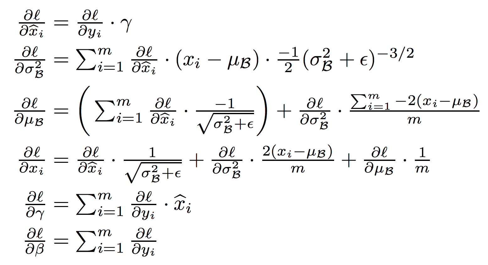
Figure 6: Original BN rule in (Ioffe & Szegedy, 2015).

It turns out that with vector notation, the update equations have a compact vector form with clear geometric meaning.

To achieve that, we first write down the vector form of forward pass of batch normalization:

$$\hat{\mathbf{f}}=P^{\perp}_{1}\mathbf{f},\quad\tilde{\mathbf{f}}{}=\hat{\mathbf{f}}/\|\hat{\mathbf{f}}\|_{\mathrm{uni}},\quad\bar{\mathbf{f}}=c_{1}\tilde{\mathbf{f}}+c_{0}\mathbf{1}=S(\mathbf{f})\mathbf{c}$$ (74)

where $\mathbf{f}$, $\hat{\mathbf{f}}$, $\tilde{\mathbf{f}}$ and $\bar{\mathbf{f}}$ are vectors of size $N$, $P^{\perp}_{1}\equiv I-\frac{\mathbf{1}\mathbf{1}^{T}}{N}$ is the projection matrix that centers the data, $\sigma=\|\mathbf{f}\|_{\mathrm{uni}}=\frac{1}{\sqrt{N}}\|\mathbf{f}\|_{2}$ and $\mathbf{c}\equiv[c_{1},c_{0}]^{T}$ are the parameters in Batch Normalization and $S(\mathbf{f})\equiv[\tilde{\mathbf{f}}{},\mathbf{1}]$ is the standardized data. Note that $S(\mathbf{f}{})^{T}S(\mathbf{f}{})=N\cdot I_{2}$ ($I_{2}$ is $2$-by-$2$ identity matrix) and thus $S(\mathbf{x})$ is an column-orthogonal $N$-by-$2$ matrix. If we put everything together, then we have:

$$BN(\mathbf{f})=c_{1}\frac{P^{\perp}_{1}\mathbf{f}}{\|P^{\perp}_{1}\mathbf{f}\|_{\mathrm{uni}}}+c_{0}\mathbf{1}$$ (75)

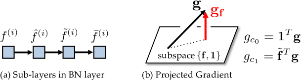
Figure 7: Analysis of Batch Normalization. (a) A Batch Normalization layer could be decomposed into three sublayers (zero-mean, unit-variance, affine). (b) The down gradient $\mathbf{g}_{\mathbf{f}}$ is a projection of input gradient $\mathbf{g}$ onto the orthogonal complementary space spanned by $\{\mathbf{f},\mathbf{1}\}$.

Using this notation, we can compute the Jacobian of batch normalization layer. Specifically, for any vector $\mathbf{f}$, we have:

$$\frac{\mathrm{d}\left(\frac{\mathbf{f}}{\|\mathbf{f}\|}\right)}{\mathrm{d}\mathbf{f}}=\frac{1}{\|\mathbf{f}\|}\left(I-\frac{\mathbf{f}\mathbf{f}^{T}}{\|\mathbf{f}\|^{2}}\right)=\frac{1}{\|\mathbf{f}\|}P^{\perp}_{\mathbf{f}}$$ (76)

where $P^{\perp}_{\mathbf{f}}$ projects a vector into the orthogonal complementary space of $\mathbf{f}$. Therefore we have:

$${J^{BN}(\mathbf{f})}=\frac{\mathrm{d}\bar{\mathbf{f}}{}}{\mathrm{d}\mathbf{f}}=c_{1}\frac{\mathrm{d}\tilde{\mathbf{f}}{}}{\mathrm{d}\mathbf{f}}=c_{1}\frac{\mathrm{d}\hat{\mathbf{f}}{}}{\mathrm{d}\mathbf{f}}\frac{\mathrm{d}\tilde{\mathbf{f}}{}}{\mathrm{d}\hat{\mathbf{f}}{}}=\frac{c_{1}}{\sigma}P^{c}_{\tilde{\mathbf{f}}{},\mathbf{1}}$$ (77)

where $P^{\perp}_{\tilde{\mathbf{f}},\mathbf{1}}=I-\frac{S(\mathbf{f})S(\mathbf{f})^{T}}{N}$ is a symmetric projection matrix that projects the input gradient to the orthogonal complement space spanned by $\tilde{\mathbf{x}}$ and $\mathbf{1}$ (Fig. 2(b)). Note that the space spanned by $\tilde{\mathbf{f}}$ and $\mathbf{1}$ is also the space spanned by $\mathbf{f}$ and $\mathbf{1}$, since $\tilde{\mathbf{f}}=(\mathbf{f}-\mu\mathbf{1})/\sigma$ can be represented linearly by $\mathbf{f}$ and $\mathbf{1}$. Therefore $P^{\perp}_{\tilde{\mathbf{f}},\mathbf{1}}=P^{\perp}_{\mathbf{f},\mathbf{1}}$.

An interesting property is that since $BN(\mathbf{f})$ returns a vector in the subspace of $\mathbf{f}$ and $\mathbf{1}$, for the $N$-by-$N$ Jacobian matrix of Batch Normalization, we have:

$${J^{BN}(\mathbf{f})}BN(\mathbf{f})={J^{BN}(\mathbf{f})}\mathbf{1}={J^{BN}(\mathbf{f})}\mathbf{f}=\mathbf{0}$$ (78)

Following the backpropagation rule, we get the following gradient update for batch normalization. If $\mathbf{g}=\partial L/\partial\bar{\mathbf{f}}$ is the gradient from top, then

$$\mathbf{g}_{\mathbf{c}}=S(\mathbf{x})^{T}\mathbf{g},\quad\quad\mathbf{g}_{\mathbf{f}}={J^{BN}(\mathbf{f})}\mathbf{g}$$ (79)

Therefore, any gradient (vector of size $N$) that is back-propagated to the input of BN layer will be automatically orthogonal to that activation (which is also a vector of size $N$). ∎

7.5.1 Conserved Quantity in Batch Normalization for ReLU activation

One can find an interesting quantity, by multiplying $g_{j}(x)$ on both side of the forward equation in Eqn. 1 and taking expectation:

$$\mathbb{E}_{x}\left[g_{j}f_{j}\right]=\mathbb{E}_{x}\left[\sum_{k\in\mathrm{ch}(j)}w_{jk}f_{k}g_{j}\right]=\sum_{k\in\mathrm{ch}(j)}w_{jk}\Delta w_{jk}$$ (80)

Using the language of differential equation, we know that:

$$\int_{0}^{t}\mathbb{E}_{x}\left[g^{(t^{\prime})}_{j}f^{(t^{\prime})}_{j}\right]\mathrm{d}t^{\prime}=E_{j}(t)-E_{j}(0)$$ (81)

where $E_{j}=\frac{1}{2}\sum_{k\in\mathrm{ch}(j)}w^{2}_{jk}=\frac{1}{2}\|W_{j\cdot}\|^{2}$. If we place Batch Normalization layer just after ReLU activation and linear layer, by BN property, since $\mathbb{E}_{x}\left[g_{j}f_{j}\right]\equiv 0$ for all iterations, the row energy $E_{j}(t)$ of weight matrix $W$ of the linear layer is conserved over time. This might be part of the reason why BN helps stabilize the training. Otherwise energy might “leak” from one layer to nearby layers.

7.6 Nonlinear versus linear

Theorem 6 (Expressibility of ReLU Nonlinearity).

Assuming $m_{\alpha}=n_{\alpha}=\mathcal{O}(\exp(\mathrm{sz}(\alpha)))$, where $\mathrm{sz}(\alpha)$ is the size of receptive field of $\alpha$. If each $P_{\alpha\beta}$ is all-vert, then: ($\omega$ is top-level receptive field)

$$\min_{W}Loss_{\mathrm{ReLU}}(W)=0,\quad\min_{W}Loss_{\mathrm{Linear}}(W)=\mathcal{O}(\exp(\mathrm{sz}(\omega)))$$ (82)

Here we define $Loss(W)\equiv\|F_{\omega}-I\|^{2}_{F}$.

Proof.

We prove that in the case of nonlinearity, there exists a weight so that the activation $F_{\alpha}=I$ for all $\alpha$. We prove by induction. The base case is trivial since we already know that $F_{\alpha}=I$ for all leaf regions.

Suppose $F_{\beta}=I$ for any $\beta\in\mathrm{ch}(\alpha)$. Since $P_{\alpha\beta}$ is all-vert, every row is a vertex of the convex hull, which means that for $i$-th row $p_{i}$, there exists a weight $\mathbf{w}_{i}$ and $b_{i}$ so that $\mathbf{w}_{i}^{T}p_{i}+b_{i}=1/|\mathrm{ch}(\alpha)|>0$ and $\mathbf{w}_{i}^{T}p_{j}+b_{i}<0$ for $j\neq i$. Put these weights and biases together into $W_{\beta\alpha}$ and we have

$$F_{\alpha}^{\mathrm{raw}}=\sum_{\beta}P_{\alpha\beta}F_{\beta}W_{\beta\alpha}=\sum_{\beta}P_{\alpha\beta}W_{\beta\alpha}$$ (83)

All diagonal elements of $F_{\alpha}^{\mathrm{raw}}$ are $1$ while all off-diagonal elements are negative. Therefore, after ReLU, $F_{\alpha}=I$. Applying induction, we get $F_{\omega}=I$ and $G_{\omega}=I-F_{\omega}=0$. Therefore, $Loss_{\mathrm{ReLU}}(W)=\|G_{\omega}\|^{2}_{F}=0$.

In the linear case, we know that $\mathrm{rank}(F_{\alpha})\leq\sum_{\beta}\mathrm{rank}(P_{\alpha\beta}F_{\beta}W_{\beta\alpha})\leq\sum_{\beta}\mathrm{rank}(F_{\beta})$, which is on the order of the size $\mathrm{sz}(\alpha)$ of $\alpha$’s receptive field (Note that the constant relies on the overlap between receptive fields). However, at the top-level, $m_{\omega}=n_{\omega}=\mathcal{O}(\exp(\mathrm{sz}(\omega)))$, i.e., the information contained in $\alpha$ is exponential with respect to the size of the receptive field. By Eckart–Young–Mirsky theorem, we know that there is a lower bound for low-rank approximation. Therefore, the loss for linear network $Loss_{\mathrm{linear}}$ is at least on the order of $m_{0}$, i.e., $Loss_{\mathrm{linear}}=\mathcal{O}(m_{\omega})$. Note that this also works if we have BN layer in-between, since BN does a linear transform in the forward pass. ∎

Theorem 7.

The following two are correct:

• If $F$ is row full rank, then $\mathrm{vert}(PF)=\mathrm{vert}(P)$.

• $PF$ is all-vert iff $P$ is all-vert.

Proof.

For (1), note that each row of $PF$ is $p_{i}^{T}F$. If $F$ is row full rank, then $F$ has pseudo-inverse $F^{\prime}$ so that $FF^{\prime}=I$. Therefore, if $p_{i}$ is not a vertex:

$$p_{i}=\sum_{j\neq i}a_{j}p_{j},\quad\sum_{j}a_{j}=1,a_{j}\geq 0,$$ (84)

then $p_{i}^{T}F$ is also not a vertex and vice versa. Therefore, $\mathrm{vert}(PF)=\mathrm{vert}(P)$. (2) follows from (1). ∎

7.7 disentangled Representation

We first start with two lemmas. Both of them have simple proofs.

Lemma 1.

Distribution representations have the following property:

• If $F^{(i)}_{\alpha}$ is disentangled, $F_{\alpha}=\sum_{i}w_{i}F^{(i)}_{\alpha}$ is also disentangled.

• If $F_{\alpha}$ is disentangled and $h$ is any per-column element-wise function, then $h(F_{\alpha})$ is disentangled.

• If $F^{(i)}_{\alpha}$ are disentangled, $h_{i}$ are per-column element-wise function, then $h_{1}(F^{(1)}_{\alpha})\circ h_{2}(F^{(2)}_{\alpha})\ldots\circ h_{n}(F^{(n)}_{\alpha})$ is disentangled.

Proof.

(1) follows from properties of tensor product. For (2) and (3), note that the $j$-th column of $F_{\alpha}$ is $F_{\alpha,:j}=\mathbf{1}\otimes\ldots\mathbf{f}_{j}\ldots\otimes\mathbf{1}$, therefore $h^{j}(F_{\alpha,:j})=\mathbf{1}\otimes\ldots h^{j}(\mathbf{f}_{j})\ldots\otimes\mathbf{1}$, and $h^{j}_{1}(F^{(1)}_{\alpha,:j})\circ h^{j}_{2}(F^{(2)}_{\alpha,:j})=\mathbf{1}\otimes\ldots h^{j}_{1}(\mathbf{f}^{(1)}_{j})\circ h^{j}_{2}(\mathbf{f}^{(2)}_{j})\ldots\otimes\mathbf{1}$. ∎

Given one child $\beta\in\mathrm{ch}(\alpha)$, denote

$$P_{S_{j}} = P_{\alpha[j]\beta[S_{j}]}=\left[\mathbb{P}(z_{\beta[S_{j}]}|z_{\alpha[j]})\right]$$ (85)

$$\mathbf{w}_{S_{j}} = W_{\beta\alpha}[S_{j},j]$$ (86)

$$\mathbf{p}_{\alpha[j]} = \left[\mathbb{P}(\alpha[j]=0),\mathbb{P}(\alpha[j]=1)\right]^{T}$$ (87)

We have $P_{S_{j}}\mathbf{1}=\mathbf{1}$ and $\mathbf{1}^{T}\mathbf{p}_{\alpha[j]}=1$. Note here for simplicity, $\mathbf{1}$ represents all-one vectors of any length, determined by the context.

Since $F_{\alpha}$ and $G_{\beta}$ are disentangled, their $j$-th column can be written as:

$$F_{\beta,:j} = \mathbf{1}\otimes\ldots\otimes\mathbf{f}_{j}\otimes\ldots\otimes\mathbf{1}$$ (88)

$$\tilde{G}_{\alpha,:j} = \mathbf{p}_{\alpha[1]}\otimes\ldots\otimes\tilde{\mathbf{g}}_{j}\otimes\ldots\otimes\mathbf{p}_{\alpha[n_{\alpha}]}$$ (89)

For simplicity, in the following proofs, we just show the case that $n_{\alpha}=2$, $n_{\beta}=3$, $z_{\alpha}=\left[z_{\alpha[1]},z_{\alpha[2]}\right]$ and $S=\{S_{1},S_{2}\}=\{\{1,2\},\{3\}\}$. We write $\mathbf{f}_{1,2}=[\mathbf{f}_{1}\otimes\mathbf{1},\mathbf{1}\otimes\mathbf{f}_{2}]$ as a 2-column matrix. The general case is similar and we omit here for brevity.

Theorem 8 (disentangled Forward).

If for each $\beta\in\mathrm{ch}(\alpha)$, $P_{\alpha\beta}$ can be written as a tensor product $P_{\alpha\beta}=\bigotimes_{i}P_{\alpha[i]\beta[S^{\alpha\beta}_{i}]}$ where $\{S^{\alpha\beta}_{i}\}$ are $\alpha\beta$-dependent disjointed set, $W_{\beta\alpha}$ is separable with respect to $\{S^{\alpha\beta}_{i}\}$, $F_{\beta}$ is disentangled, then $F_{\alpha}$ is also disentangled (with/without ReLU /Batch Norm).

Proof.

For a certain $\beta\in\mathrm{ch}(\alpha)$, we first compute the quantity $P_{\alpha\beta}F_{\beta}$:

$$P_{\alpha\beta}F_{\beta}=\left(P_{1,2}\otimes P_{3}\right)\left[\mathbf{f}_{1,2}\otimes\mathbf{1},\ \ \mathbf{1}\otimes\mathbf{f}_{3}\right]=\left[P_{1,2}\mathbf{f}_{1,2}\otimes\mathbf{1},\ \ \mathbf{1}\otimes P_{3}\mathbf{f}_{3}\right]$$ (90)

Therefore, the forward information sent from $\beta$ to $\alpha$ is:

$$F^{\mathrm{raw}}_{\beta\rightarrow\alpha} = P_{\alpha\beta}F_{\beta}W_{\beta\alpha}=\left[P_{1,2}\mathbf{f}_{1,2}\otimes\mathbf{1},\ \ \mathbf{1}\otimes P_{3}\mathbf{f}_{3}\right]\left[\begin{array}[]{cc}\mathbf{w}_{1,2}&0\\ 0&\mathbf{w}_{3}\end{array}\right]$$ (93)

$$= \left[P_{1,2}\mathbf{f}_{1,2}\mathbf{w}_{1,2}\otimes\mathbf{1},\ \ \mathbf{1}\otimes P_{3}\mathbf{f}_{3}\mathbf{w}_{3}\right]$$ (94)

Note that both $P_{1,2}\mathbf{f}_{1,2}\mathbf{w}_{1,2}$ and $P_{3}\mathbf{f}_{3}\mathbf{w}_{3}$ are 2-by-1 vectors. Therefore, for each $\beta\in\mathrm{ch}(\alpha)$, $F^{\mathrm{raw}}_{\beta\rightarrow\alpha}$ is disentangled. By Lemma 1, both $F^{\mathrm{raw}}_{\alpha}=\sum_{\beta\in\mathrm{ch}(\alpha)}F^{\mathrm{raw}}_{\beta\rightarrow\alpha}$ and the nonlinear response $F_{\alpha}$ are disentangled. By Eqn. 12, the forward pass of Batch Norm is a per-column element-wise function, so BN also preserves disentangledness. ∎

Theorem 9 (Separable Weight Update).

If $P_{\alpha\beta}=\bigotimes_{i}P_{\alpha[i]\beta[S_{i}]}$, both $F_{\beta}$ and $\tilde{G}_{\alpha}$ are disentangled, $\mathbf{1}^{T}\tilde{G}_{\alpha}=\mathbf{0}$, then the gradient update $\Delta W_{\beta\alpha}$ is separable with respect to $\{S_{i}\}$.

Proof.

Following Eqn. 59 and Eqn. 90, we have:

$$\Delta W_{\beta\alpha} = \left(P_{\alpha\beta}F_{\beta}\right)^{T}\tilde{G}_{\alpha}$$ (95)

$$= \left[\begin{array}[]{c}(P_{1,2}\mathbf{f}_{1,2})^{T}\otimes\mathbf{1}^{T}\\ \mathbf{1}^{T}\otimes(P_{3}\mathbf{f}_{3})^{T}\end{array}\right]\left[\tilde{\mathbf{g}}_{1}\otimes\mathbf{p}_{\alpha[2]},\ \ \mathbf{p}_{\alpha[1]}\otimes\tilde{\mathbf{g}}_{2}\right]$$ (98)

$$= \left[\begin{array}[]{cc}(P_{1,2}\mathbf{f}_{1,2})^{T}\tilde{\mathbf{g}}_{1}&(P_{1,2}\mathbf{f}_{1,2})^{T}\mathbf{p}_{\alpha[1]}\otimes\mathbf{1}^{T}\tilde{\mathbf{g}}_{2}\\ \mathbf{1}^{T}\tilde{\mathbf{g}}_{1}\otimes(P_{3}\mathbf{f}_{3})^{T}\mathbf{p}_{\alpha[2]}&(P_{3}\mathbf{f}_{3})^{T}\tilde{\mathbf{g}}_{2}\\ \end{array}\right]$$ (101)

Since $\mathbf{1}^{T}\tilde{G}_{\alpha}=\mathbf{0}$, we have for any $j$, $\mathbf{1}^{T}\tilde{G}_{\alpha,:j}=0$ and thus $\mathbf{1}^{T}\tilde{\mathbf{g}}_{j}=0$. Therefore,

$$\Delta W_{\beta\alpha}=\mathrm{diag}\left((P_{1,2}\mathbf{f}_{1,2})^{T}\tilde{\mathbf{g}}_{1},\ \ (P_{3}\mathbf{f}_{3})^{T}\tilde{\mathbf{g}}_{2}\right)$$ (102)

which is separable with respect to $S$. In particular:

$$\Delta\mathbf{w}_{1,2}=(P_{1,2}\mathbf{f}_{1,2})^{T}\tilde{\mathbf{g}}_{1},\quad\Delta\mathbf{w}_{3}=(P_{3}\mathbf{f}_{3})^{T}\tilde{\mathbf{g}}_{2}$$ (103)

∎

7.7.1 Discussion about backpropagation of disentangled gradient

One problem remains. If $\{\tilde{G}_{\alpha}\}_{\alpha\in\mathrm{pa}(\beta)}$ are all disentangled, whether $\tilde{G}_{\beta}$ is disentangled? We can try computing the following quality:

$$\tilde{G}^{\mathrm{raw}}_{\alpha\rightarrow\beta} = P_{\alpha\beta}^{T}\tilde{G}_{\alpha}W_{\beta\alpha}^{T}$$ (104)

$$= \left(P^{T}_{1,2}\otimes P^{T}_{3}\right)\left[\tilde{\mathbf{g}}_{1}\otimes\mathbf{p}_{\alpha[2]},\ \ \mathbf{p}_{\alpha[1]}\otimes\tilde{\mathbf{g}}_{2}\right]\left[\begin{array}[]{cc}\mathbf{w}^{T}_{1,2}&0\\ 0&\mathbf{w}^{T}_{3}\end{array}\right]$$ (107)

$$= \left[P_{1,2}^{T}\tilde{\mathbf{g}}_{1}\otimes\mathbf{p}_{\beta[3]},\ \ \mathbf{p}_{\beta[1,2]}\otimes P_{3}^{T}\tilde{\mathbf{g}}_{2}\right]\left[\begin{array}[]{cc}\mathbf{w}^{T}_{1,2}&0\\ 0&\mathbf{w}^{T}_{3}\end{array}\right]$$ (110)

$$= \left[P_{1,2}^{T}\tilde{\mathbf{g}}_{1}\mathbf{w}^{T}_{1,2}\otimes\mathbf{p}_{\beta[3]},\ \ \mathbf{p}_{\beta[1,2]}\otimes P_{3}^{T}\tilde{\mathbf{g}}_{2}\mathbf{w}^{T}_{3}\right]$$ (111)

Note that here we use the following equality from total probability rule:

$$P_{3}^{T}\mathbf{p}_{\alpha[2]}=\mathbf{p}_{\beta[3]},\quad P_{1,2}^{T}\mathbf{p}_{\alpha[1]}=\mathbf{p}_{\beta[1,2]}$$ (112)

where $\mathbf{p}_{\beta[1,2]}$ is a 4-by-1 vector:

$$\mathbf{p}_{\beta[1,2]}=\left[\begin{array}[]{c}\mathbb{P}(z_{\beta[1]}=0,z_{\beta[2]}=0)\\ \mathbb{P}(z_{\beta[1]}=0,z_{\beta[2]}=1)\\ \mathbb{P}(z_{\beta[1]}=1,z_{\beta[2]}=0)\\ \mathbb{P}(z_{\beta[1]}=1,z_{\beta[2]}=1)\end{array}\right]$$ (113)

Note that the ordering of these joint probability corresponds to the column order of $P_{1,2}$.

Now with this example, we see that the backward case ( Eqn. 112) is very different from the forward case (Eqn. 94), in which $\tilde{G}^{\mathrm{raw}}_{\alpha\rightarrow\beta}$ is no longer disentangled. Indeed, $P_{1,2}^{T}\tilde{\mathbf{g}}_{1}\mathbf{w}^{T}_{1,2}$ is a 2-column matrix and $\mathbf{p}_{\beta[1,2]}$ is not a rank-1 tensor anymore. Intuitively this makes sense, if two low-level attributes have very similar behaviors, there is no way to distinguish the two via backpropagation.

Note that we also cannot assume independence: $\mathbf{p}_{\beta[1,2]}=\mathbf{p}_{\beta[1]}\otimes\mathbf{p}_{\beta[2]}$ since the independence property is in general not carried from layer to layer.

For general cases, $\tilde{G}^{\mathrm{raw}}_{\alpha\rightarrow\beta}$ takes the following form:

$$\tilde{G}^{\mathrm{raw}}_{\alpha\rightarrow\beta}=\left[P_{S^{\alpha\beta}_{1}}^{T}\tilde{\mathbf{g}}^{\alpha}_{1}\mathbf{w}_{S^{\alpha\beta}_{1}}^{T}\otimes\bigotimes_{j=2}^{n_{\alpha}}\mathbf{p}_{\beta[S^{\alpha\beta}_{j}]},\quad\mathbf{p}_{\beta[S^{\alpha\beta}_{1}]}\otimes P_{S^{\alpha\beta}_{2}}^{T}\tilde{\mathbf{g}}^{\alpha}_{2}\mathbf{w}_{S^{\alpha\beta}_{2}}^{T}\otimes\bigotimes_{j=3}^{n_{\alpha}}\mathbf{p}_{\beta[S^{\alpha\beta}_{j}]},\quad\ldots\right]$$ (114)

One hope here is that if we consider $\sum_{\alpha\in\mathrm{pa}(\beta)}\tilde{G}^{\mathrm{raw}}_{\alpha\rightarrow\beta}$, the summation over parent $\alpha$ could lead to a better structure, even for individual $\alpha$, $P_{S_{1}}^{T}\tilde{\mathbf{g}}^{\alpha}_{1}\mathbf{w}_{S_{1}}^{T}$ is not 1-order tensor. For example, if $S^{\alpha\beta}_{j}=S_{j}$, then for the first column in $S_{1}$, due to $\mathbf{1}^{T}\tilde{\mathbf{g}}_{j}=0$, we know that:

$$\sum_{\alpha\in\mathrm{pa}(\beta)}P_{\alpha,S_{1}}^{T}\tilde{\mathbf{g}}^{\alpha}_{1}\mathbf{w}_{\alpha,S_{1}[1]}^{T}=\sum_{\alpha\in\mathrm{pa}(\beta)}c_{\alpha}(\mathbf{v}^{+}_{\alpha,S_{1}}-\mathbf{v}^{-}_{\alpha,S_{1}})$$ (115)

where $\mathbf{v}^{+}_{\alpha,S_{1}}=\mathbb{P}(z_{\beta[S_{1}]}|z_{\alpha[1]}=1)$ and $\mathbf{v}^{-}_{\alpha,S_{1}}=\mathbb{P}(z_{\beta[S_{1}]}|z_{\alpha[1]}=0)$ and $P_{\alpha,S_{i}}=\left[\begin{array}[]{c}\mathbf{v}^{-}_{\alpha,S_{1}}\\ \mathbf{v}^{+}_{\alpha,S_{1}}\end{array}\right]$. If each $\alpha\in\mathrm{pa}(\beta)$ is informative in a diverse way, and $|S_{1}|$ is relatively small (e.g., 4), then $\mathbf{v}^{+}_{\alpha,S_{1}}-\mathbf{v}^{-}_{\alpha,S_{1}}\neq\mathbf{0}$ and spans the probability space of dimension $2^{|S_{1}|}-1$. Then we can always find $c_{\alpha}$ (or equivalently, weights) so that Eqn. 115 becomes rank-1 tensor (or disentangled). Besides, the gating $D_{\beta}$, which is disentangled as it is an element-wise function of $F_{\beta}$, will also play a role in regularizing $\tilde{G}_{\beta}$.

We will leave this part to future work.

References

- Amit et al. (1985) Daniel J Amit, Hanoch Gutfreund, and Haim Sompolinsky. Spin-glass models of neural networks. Physical Review A, 32(2):1007, 1985.
- Bau et al. (2017) David Bau, Bolei Zhou, Aditya Khosla, Aude Oliva, and Antonio Torralba. Network dissection: Quantifying interpretability of deep visual representations. CVPR, 2017.
- Brutzkus & Globerson (2017) Alon Brutzkus and Amir Globerson. Globally optimal gradient descent for a convnet with gaussian inputs. ICML, 2017.
- Choromanska et al. (2015a) Anna Choromanska, Mikael Henaff, Michael Mathieu, Gérard Ben Arous, and Yann LeCun. The loss surfaces of multilayer networks. In Artificial Intelligence and Statistics, pp. 192–204, 2015a.
- Choromanska et al. (2015b) Anna Choromanska, Yann LeCun, and Gérard Ben Arous. Open problem: The landscape of the loss surfaces of multilayer networks. In Conference on Learning Theory, pp. 1756–1760, 2015b.
- Dauphin et al. (2014) Yann N Dauphin, Razvan Pascanu, Caglar Gulcehre, Kyunghyun Cho, Surya Ganguli, and Yoshua Bengio. Identifying and attacking the saddle point problem in high-dimensional non-convex optimization. In Advances in neural information processing systems, pp. 2933–2941, 2014.
- Du et al. (2017) Simon S Du, Chi Jin, Jason D Lee, Michael I Jordan, Aarti Singh, and Barnabas Poczos. Gradient descent can take exponential time to escape saddle points. In Advances in Neural Information Processing Systems, pp. 1067–1077, 2017.
- Du et al. (2018) Simon S Du, Jason D Lee, Yuandong Tian, Barnabas Poczos, and Aarti Singh. Gradient descent learns one-hidden-layer cnn: Don’t be afraid of spurious local minima. ICML, 2018.
- Goodfellow et al. (2014) Ian J Goodfellow, Oriol Vinyals, and Andrew M Saxe. Qualitatively characterizing neural network optimization problems. arXiv preprint arXiv:1412.6544, 2014.
- Hardt & Ma (2017) Moritz Hardt and Tengyu Ma. Identity matters in deep learning. ICLR, 2017.
- He et al. (2016) Kaiming He, Xiangyu Zhang, Shaoqing Ren, and Jian Sun. Deep residual learning for image recognition. In Proceedings of the IEEE conference on computer vision and pattern recognition, pp. 770–778, 2016.
- Ioffe & Szegedy (2015) Sergey Ioffe and Christian Szegedy. Batch normalization: Accelerating deep network training by reducing internal covariate shift. ICML, 2015.
- Kawaguchi (2016) Kenji Kawaguchi. Deep learning without poor local minima. In Advances in Neural Information Processing Systems, pp. 586–594, 2016.
- Keskar et al. (2017) Nitish Shirish Keskar, Dheevatsa Mudigere, Jorge Nocedal, Mikhail Smelyanskiy, and Ping Tak Peter Tang. On large-batch training for deep learning: Generalization gap and sharp minima. ICLR, 2017.
- Kohler et al. (2018) Jonas Kohler, Hadi Daneshmand, Aurelien Lucchi, Ming Zhou, Klaus Neymeyr, and Thomas Hofmann. Towards a theoretical understanding of batch normalization. arXiv preprint arXiv:1805.10694, 2018.
- Krizhevsky et al. (2012) Alex Krizhevsky, Ilya Sutskever, and Geoffrey E Hinton. Imagenet classification with deep convolutional neural networks. In Advances in neural information processing systems, pp. 1097–1105, 2012.
- Li et al. (2017) Hao Li, Zheng Xu, Gavin Taylor, and Tom Goldstein. Visualizing the loss landscape of neural nets. arXiv preprint arXiv:1712.09913, 2017.
- Mehta & Schwab (2014) Pankaj Mehta and David J Schwab. An exact mapping between the variational renormalization group and deep learning. arXiv preprint arXiv:1410.3831, 2014.
- Mei et al. (2016) Song Mei, Yu Bai, and Andrea Montanari. The landscape of empirical risk for non-convex losses. arXiv preprint arXiv:1607.06534, 2016.
- Poole et al. (2016) Ben Poole, Subhaneil Lahiri, Maithra Raghu, Jascha Sohl-Dickstein, and Surya Ganguli. Exponential expressivity in deep neural networks through transient chaos. In Advances in neural information processing systems, pp. 3360–3368, 2016.
- Safran & Shamir (2017) Itay Safran and Ohad Shamir. Spurious local minima are common in two-layer relu neural networks. CoRR, abs/1712.08968, 2017. URL http://arxiv.org/abs/1712.08968.
- Saxe et al. (2013) Andrew M Saxe, James L McClelland, and Surya Ganguli. Exact solutions to the nonlinear dynamics of learning in deep linear neural networks. arXiv preprint arXiv:1312.6120, 2013.
- Silver et al. (2016) David Silver, Aja Huang, Chris J Maddison, Arthur Guez, Laurent Sifre, George Van Den Driessche, Julian Schrittwieser, Ioannis Antonoglou, Veda Panneershelvam, Marc Lanctot, et al. Mastering the game of go with deep neural networks and tree search. nature, 529(7587):484, 2016.
- Silver et al. (2017) David Silver, Julian Schrittwieser, Karen Simonyan, Ioannis Antonoglou, Aja Huang, Arthur Guez, Thomas Hubert, Lucas Baker, Matthew Lai, Adrian Bolton, et al. Mastering the game of go without human knowledge. Nature, 550(7676):354, 2017.
- Simonyan & Zisserman (2014) Karen Simonyan and Andrew Zisserman. Very deep convolutional networks for large-scale image recognition. arXiv preprint arXiv:1409.1556, 2014.
- Su et al. (2014) Weijie Su, Stephen Boyd, and Emmanuel Candes. A differential equation for modeling nesterov’s accelerated gradient method: Theory and insights. In Advances in Neural Information Processing Systems, pp. 2510–2518, 2014.
- Tian (2017) Yuandong Tian. An analytical formula of population gradient for two-layered relu network and its applications in convergence and critical point analysis. ICML, 2017.
- Tian & Zhu (2016) Yuandong Tian and Yan Zhu. Better computer go player with neural network and long-term prediction. ICLR, 2016.
- Venturi et al. (2018) Luca Venturi, Afonso Bandeira, and Joan Bruna. Neural networks with finite intrinsic dimension have no spurious valleys. arXiv preprint arXiv:1802.06384, 2018.
- Zhang et al. (2016) Chiyuan Zhang, Samy Bengio, Moritz Hardt, Benjamin Recht, and Oriol Vinyals. Understanding deep learning requires rethinking generalization. ICLR, 2016.