Minimax Lower Bounds for $\mathcal{H}_{\infty}$-Norm Estimation

Abstract

The problem of estimating the $\mathcal{H}_{\infty}$-norm of an LTI system from noisy input/output measurements has attracted recent attention as an alternative to parameter identification for bounding unmodeled dynamics in robust control. In this paper, we study lower bounds for $\mathcal{H}_{\infty}$-norm estimation under a query model where at each iteration the algorithm chooses a bounded input signal and receives the response of the chosen signal corrupted by white noise. We prove that when the underlying system is an FIR filter, $\mathcal{H}_{\infty}$-norm estimation is no more efficient than model identification for passive sampling. For active sampling, we show that norm estimation is at most a factor of $\log{r}$ more sample efficient than model identification, where $r$ is the length of the filter. We complement our theoretical results with experiments which demonstrate that a simple non-adaptive estimator of the norm is competitive with state-of-the-art adaptive norm estimation algorithms.

1 Introduction

Recently, many researchers have proposed algorithms for estimating the $\mathcal{H}_{\infty}$-norm of a linear time-invariant (LTI) filter from input/output data [16, 18, 12, 10, 9, 11]. A common property of these algorithms is eschewing model parameter estimation for directly estimating either the worst case $\ell_{2}$-input signal [18, 12] or the maximizing frequency [9, 11]. One of the major motivations behind these algorithms is sample efficiency: since the $\mathcal{H}_{\infty}$-norm is a scalar estimate whereas the number of model parameters can be very large and possibly infinite, intuitively one expects that norm estimation can be performed using substantially fewer samples compared with model estimation.

In this paper, we study the fundamental limits of estimating the $\mathcal{H}_{\infty}$-norm of a finite impulse response (FIR) filter, and compare to known bounds for FIR model estimation. We show that for passive algorithms which do not adapt their inputs in response to the result of previous queries, it is no more efficient to estimate the $\mathcal{H}_{\infty}$-norm than to estimate the model. For active algorithms which do adapt their inputs, we show that compared to model estimation, norm estimation is only at most a $\log{r}$ factor more efficient when the underlying model is a length $r$ FIR filter. Our analysis raises an interesting open question: whether or not there there exists an active sampling strategy which attains our stated lower bound.

Based on our theoretical findings, we study the empirical performance of several existing adaptive algorithms compared to a simple (non-adaptive) estimator which first fits a model via least-squares and then returns the norm of the model. Surprisingly, we find that the current adaptive methods do not perform significantly better than the simple estimator.

2 Related Work

Data-driven methods for estimating the $\mathcal{H}_{\infty}$-norm of an LTI system fall into roughly two major approaches: (a) estimating the worst case $\ell_{2}$-signal via a power-iteration type algorithm [18, 12, 10] and (b) discretizing the interval $[0,2\pi)$ and searching for the maximizing frequency [9, 11].

Algorithms that rely on power iteration take advantage of a clever time-reversal trick introduced by Wahlberg et al. [18], which allows one to query the adjoint system $G^{*}$ with only input/output access to the original system $G$. One issue with these methods is that the rate of convergence of the top singular value of the truncated Toeplitz matrix to the $\mathcal{H}_{\infty}$-norm of the system is typically $O(1/n^{2})$ (c.f. [2]), but the constant hidden in the $O(\cdot)$ notation can be quite large as pointed out by [15]. A non-asymptotic analysis of the statistical quality of the norm estimate returned by the power iteration remains an open question; asymptotic results can be found in [12].

The algorithms developed in [9, 11] based on discretizing the frequencies $[0,2\pi)$ are rooted in ideas from the multi-armed bandit literature. Here, each frequency can be treated as either an “arm” or an “expert”, and an adaptive algorithm such as Thompson sampling [9] or multiplicative weights [11] is applied. While sharp regret analysis for bandits has been developed by the machine learning and statistics communities [3], one of the barriers to applying this analysis is a lack of a sharp theory for the level of discretization required. In practice, the number of grid points is a parameter that must be appropriately tuned for the problem at hand.

The problem of estimating the model parameters of a LTI system with model error measured in $\mathcal{H}_{\infty}$-norm is studied by [14], and in $\ell_{p}$-norms by [5]. For the FIR setting, [14] gives matching upper and lower bounds for identification in $\mathcal{H}_{\infty}$-norm. These bounds will serve as a baseline for us to compare our bounds with in the norm estimation setting. Helmicki et al. [7] provide lower bounds for estimating both a model in $\mathcal{H}_{\infty}$-norm and its frequency response at a particular frequency in a query setting where the noise is worst-case. In this work we consider a less conservative setting with stochastic noise. Müller et al. [9] prove an asymptotic regret lower bound over algorithms that sample only one frequency at every iteration. Their notion of regret is however defined with respect to the best frequency in a fixed discrete grid and not the $\mathcal{H}_{\infty}$-norm. As we discuss in Section 3.2, this turns out to be a subtle but important distinction.

3 Problem Setup and Main Results

In this section we formulate the problem under consideration and state our main results. We fix a filter length $r$ and consider an unknown length $r$ causal FIR filter $H(g):=\sum_{k=0}^{r-1}g_{k}z^{-k}$ with $g\in\mathbb{C}^{r}$. We study the following time-domain input/output query model for $H(g)$: for $N$ rounds, we first choose an input $u_{t}\in\mathbb{C}^{r}$ such that $\lVert u_{t}\rVert_{2}\leq M$, and then we observe a sample $y_{t}\sim\mathcal{N}(T(g)u_{t},\sigma^{2}I)$, where $T(g)$ denotes the $r\times r$ upper left section of the semi-infinite Toeplitz matrix induced by treating $g$ as an element of $\ell_{2}$ . By $\mathcal{N}(\mu,\sigma^{2}I)$ for a complex $\mu\in\mathbb{C}^{r}$ we mean we observe $(\mathrm{Re}(\mu)+\xi_{1})+j(\mathrm{Im}(\mu)+\xi_{2})$ where $\xi_{i}\sim\mathcal{N}(0,\sigma^{2}I)$ and are independent.

After these $N$ rounds, we are to return an estimate $\widehat{H}\in\mathbb{R}$ of the norm $\lVert H(g)\rVert_{\mathcal{H}_{\infty}}$ based on the collected data $(u_{1},y_{1},...,u_{N},y_{N})$. The expected risk of any algorithm for this problem is measured as $\mathbb{E}[|\widehat{H}-\lVert H(g)\rVert_{\mathcal{H}_{\infty}}|]$, where the expectation is taken with respect to both the randomness of the algorithm and the noise of the outputs $y_{t}$.

Our results distinguish between passive and active algorithms. A passive algorithm is one in which the distribution of the input $u_{t}$ at time $t$ is independent of the history $(u_{1},y_{1},...,u_{t-1},y_{t-1})$. An active algorithm is one where the distribution of $u_{t}$ is allowed to depend on this history.

Given this setup, our first result is a minimax lower bound for the risk attained by any passive algorithm.

Theorem 1 (Passive lower bound).

Fix a $\gamma>0$. Let $r\geq c$ for a universal constant $c>0$ and $N\geq\mathrm{poly}(r,M,1/\gamma)$. We call a passive algorithm $\mathcal{A}$ admissible if the matrix $\frac{1}{N}\sum_{t=1}^{N}\mathbb{E}_{u_{t}}[T(u_{t})^{*}T(u_{t})]\succeq\gamma I$. We have the following minimax lower bound on the risk of any passive admissible algorithm $\mathcal{A}$:

$$\inf_{\mathcal{A}}\sup_{\theta\in\mathbb{C}^{r}}\mathbb{E}[|\widehat{H}_{\mathcal{A}}-\lVert H(g)\rVert_{\mathcal{H}_{\infty}}|]\geq C^{\prime}\frac{\sigma}{M}\sqrt{\frac{r\log{r}}{N}}\>.$$ (3.1)

Here, $C^{\prime}$ is a universal constant. We note the form of the $\mathrm{poly}(r,M,1/\gamma)$ can be recovered from the proof.

The significance of Theorem 1 is due to the fact that under our query model, one can easily produce an estimate $\widehat{g}\in\mathbb{C}^{r}$ such that $\mathbb{E}[\lVert H(\widehat{g})-H(g)\rVert_{\mathcal{H}_{\infty}}]\leq C^{\prime\prime}\frac{\sigma}{M}\sqrt{\frac{r\log{r}}{N}}$, for instance by setting $u_{t}=Me_{1}$ where $e_{1}$ is the first standard basis vector (see e.g. Theorem 1.1 of [14]). That is, for passive algorithms the number of samples to estimate the $r$ model parameters is equal (up to constants) to the number of samples needed to estimate the $\mathcal{H}_{\infty}$-norm, at least for the worst-case. The situation changes slightly when we look at active algorithms.

Theorem 2 (Active lower bound).

The following minimax lower bound on the risk of any active algorithm $\mathcal{A}$ holds:

$$\inf_{\mathcal{A}}\sup_{\theta\in\mathbb{C}^{r}}\mathbb{E}[|\widehat{H}_{\mathcal{A}}-\lVert H(g)\rVert_{\mathcal{H}_{\infty}}|]\geq C^{\prime}\frac{\sigma}{M}\sqrt{\frac{r}{N}}\>.$$ (3.2)

Here, $C^{\prime}$ is a universal constant.

We see in the active setting that the lower bound is weakened by a logarithmic factor in $r$. This bound shows that for low SNR regimes when $M\ll\sqrt{r}$, the gains of being active are minimal in the worst case. On the other hand, for high SNR regimes when $M\gg\sqrt{r}$, the gains are potentially quite substantial. We are unaware of any algorithm that provably achieves the active lower bound; it is currently unclear whether or not the lower bound is loose, or if more careful design/analysis is needed to find a better active algorithm. However, in Section 3.2 we discuss special cases of FIR filters for which the lower bound in Theorem 2 is not improvable.

We note that our proof draws heavily on techniques used to prove minimax lower bounds for functional estimation, specifically in estimating the $\ell_{\infty}$-norm of a unknown mean vector in the Gaussian sequence model. An excellent overview of these techniques is given in Chapter 22 of [19].

3.1 Hypothesis testing and sector conditions

An application that is closely related to estimating the $\mathcal{H}_{\infty}$-norm is testing whether or not the $\mathcal{H}_{\infty}$-norm exceeds a certain fixed threshold $\tau$. Specifically, consider a test statistic $\psi\in\{0,1\}$ that discriminates between the two alternatives $H_{0}:\lVert H(g)\rVert_{\mathcal{H}_{\infty}}\leq\tau$ and $H_{1}:\lVert H(g)\rVert_{\mathcal{H}_{\infty}}>\tau$. This viewpoint is useful because it encompasses testing for more fine-grained characteristics of the Nyquist plot $H(\omega)$ via simple transformations. For instance, given $-\infty<a<0<b<+\infty$, one may test if $H(\omega)$ is contained within a circle in the complex plane centered at $(a+b)/2+0j$ with radius $(b-a)/2$ by equivalently checking if the $\mathcal{H}_{\infty}$-norm of the system $H(g)-(a+b)/2$ is less than $(b-a)/2$; this is known as the $[a,b]$-sector condition [6].

Due to the connection between estimation and hypothesis testing, our results also give lower bounds on the sum of the Type-I and Type-II errors of any test $\psi$ discriminating between the hypothesis $H_{0}$ and $H_{1}$. Specifically, $\Omega(\frac{\sigma^{2}r\log{r}}{\tau^{2}M})$ queries in the passive case (when $\tau$ is sufficiently small) and $\Omega(\frac{\sigma^{2}r}{\tau^{2}M})$ queries in the active case are necessary for any test to have Type-I and Type-II error less than a constant probability.

3.2 Shortcomings of discretization

In order to close the gap between the upper and lower bounds, one needs to explicitly deal with the continuum of frequencies on $[0,2\pi)$; here we argue that if the maximizing frequency is known a-priori to lie in discrete set of points, then the lower bound is sharp.

Suppose we consider a slightly different query model, where at each time $t$ the algorithm chooses a frequency $\omega_{t}\in[0,2\pi)$ and receives $y_{t}\sim\mathcal{N}(H(\omega_{t}),1)$. For simplicity let us also assume that the $\mathcal{H}_{\infty}$-norm is bounded by one. Note that by slightly enlarging $T(g)$ to the $2r\times 2r$ upper left triangle, we can emulate this query model by using a normalized complex sinusoid with frequency $\omega_{t}$.

If the maximizing frequency for the $\mathcal{H}_{\infty}$-norm of the underlying system is located on the grid $\{2\pi k/r\}_{k=0}^{r-1}$ and its phase is known, this problem immediate reduces to a standard $r$-arm multi-armed bandit (MAB) problem where each arm is associated with a point on the grid. For this family of instances, the following active algorithm has expected risk upper bounded by $\sqrt{r/N}$ times a constant:

1. Run a MAB algorithm that is optimal in the stochastic setting (such as MOSS [1]) for $N/2$ iterations, with each of the $r$ arms associated to a frequency $2\pi k/r$.

2. Sample an index $I\in\{1,...,r\}$ where:

   $$\mathbb{P}(I=i)=\frac{\text{\# number of times arm $i$ was pulled}}{N/2}\>.$$

3. Query $\omega_{I}$ for $N/2$ times and return the sample mean.

More generally, for any grid of frequencies $\{\omega_{k}\}$ such that the number of grid points is $O(r)$, this algorithm obtains $O(\sqrt{r/N})$ expected risk. Hence the lower bound of Theorem 2 is actually sharp with respect to these instances.

Therefore, the issue that needs to be understood is whether or not the continuum of frequencies on $[0,2\pi)$ fundamentally requires additional sample complexity compared to a fixed discrete grid. Note that a naïve discretization argument is insufficient here. For example, it is known (see e.g. Lemma 3.1 of [14]) that by choosing $P$ equispaced frequencies one obtains a discretization error bounded by $O(r/P)$, e.g. $\lVert H(g)\rVert_{\mathcal{H}_{\infty}}-|H(\omega_{k})|\leq O(r/P)$ for the largest $\omega_{k}$. This bound is too weak, however, since it requires that the number of arms scale as $O(r/\varepsilon)$ in order to obtain a risk bounded by $\varepsilon$; in terms of $N$, the risk would scale $O(1/N^{1/3})$.

To summarize, if one wishes to improve the active lower bound to match the rate given by Theorem 1, one needs to consider a prior distribution over hard instances where the support of the maximizing frequency is large (possibly infinite) compared to $r$. On the other hand, if one wishes to construct an algorithm achieving the rate of Theorem 2, then one will need to understand the function $\omega\mapsto|H(\omega)|$ at a much finer resolution than Lipschitz continuity.

4 Proof of Main Results

The proof of Theorem 1 and Theorem 2 both rely on a reduction to Bayesian hypothesis testing. While this reduction is standard in the statistics and machine learning communities (see e.g. Chapter 2 of [13]), we briefly outline it here, as we believe these techniques are not as widely used in the controls literature.

First, let $\pi_{1},\pi_{2}$ be two prior distributions on $\mathbb{C}^{r}$. Suppose that for all $\theta_{1}\in\pi_{1}$ we have $\lVert H(\theta_{1})\rVert_{\mathcal{H}_{\infty}}=0$ and for all $\theta_{2}\in\pi_{2}$ we have $\lVert H(\theta_{2})\rVert_{\mathcal{H}_{\infty}}=2c$ for some $c>0$. Let $\mathbb{P}_{\pi_{i}}$ denote the joint distribution of $(u_{1},y_{1},...,u_{N},y_{N})$, which combines the prior distribution $\pi_{i}$ with the observation model. Then,

$$\sup_{\theta\in\mathbb{C}^{r}}\mathbb{E}[|\widehat{H}-\lVert H(\theta)\rVert_{\mathcal{H}_{\infty}}|] \geq c\sup_{\theta\in\mathbb{C}^{r}}\mathbb{P}_{\theta}(|\widehat{H}-\lVert H(\theta)\rVert_{\mathcal{H}_{\infty}}|\geq c)$$

$$\geq c\max_{i=1,2}\left\{\int\mathbb{P}_{\theta}(|\widehat{H}-\lVert H(\theta)\rVert_{\mathcal{H}_{\infty}}|\geq c)\;\pi_{i}(d\theta)\right\}$$

$$\geq\frac{c}{2}\left(\mathbb{P}_{\pi_{1}}(|\widehat{H}|\geq c)+\mathbb{P}_{\pi_{2}}(|\widehat{H}-2c|\geq c)\right)$$

$$\geq\frac{c}{2}\left(\mathbb{P}_{\pi_{1}}(|\widehat{H}|\geq c)+\mathbb{P}_{\pi_{2}}(|\widehat{H}|<c)\right)$$

$$\geq\frac{c}{2}(1-d_{\mathrm{tv}}(\mathbb{P}_{\pi_{1}},\mathbb{P}_{\pi_{2}}))\>,$$

where for two measures $\mathbb{P},\mathbb{Q}$ we define the total-variation (TV) distance as $d_{\mathrm{tv}}(\mathbb{P},\mathbb{Q})=\sup_{A}|\mathbb{P}(A)-\mathbb{Q}(A)|$. Hence, if one can construct two prior distributions $\pi_{1},\pi_{2}$ with the aforementioned properties and furthermore show that $d_{\mathrm{tv}}(\mathbb{P}_{\pi_{1}},\mathbb{P}_{\pi_{2}})\leq 1/2$, then one deduces that the minimax risk is lower bounded by $c/4$. This technique is generally known as Le Cam’s method, and will be our high-level proof strategy.

As working directly with the TV distance is often intractable, one typically computes upper bounds to the TV distance. We choose to work with both the KL-divergence and the $\chi^{2}$-divergence. The KL-divergence is defined as $d_{\mathrm{kl}}(\mathbb{P},\mathbb{Q})=\int\log\left(\frac{d\mathbb{P}}{d\mathbb{Q}}\right)\>d\mathbb{P}$, and the $\chi^{2}$-divergence is defined as $d_{\mathrm{\chi^{2}}}(\mathbb{P},\mathbb{Q})=\int\left(\frac{d\mathbb{P}}{d\mathbb{Q}}-1\right)^{2}\;d\mathbb{Q}$ (we assume that $\mathbb{P}\ll\mathbb{Q}$ so these quantities are well-defined). One has the standard inequalities $d_{\mathrm{tv}}(\mathbb{P},\mathbb{Q})\leq\sqrt{\frac{1}{2}d_{\mathrm{kl}}(\mathbb{P},\mathbb{Q})}$ and $d_{\mathrm{tv}}(\mathbb{P},\mathbb{Q})\leq\sqrt{d_{\mathrm{\chi^{2}}}(\mathbb{P},\mathbb{Q})}$ [13].

4.1 Proof of passive lower bound (Theorem 1)

The main reason for working with the $\chi^{2}$-divergence is that it operates nicely with mixture distributions, as illustrated by the following lemma.

Lemma 1 (see e.g. Lemma 22.1 of [19]).

Let $\Theta$ be a parameter space and for each $\theta\in\Theta$ let $\mathbb{P}_{\theta}$ be a measure over $\mathcal{X}$ indexed by $\theta$. Fix a measure $\mathbb{Q}$ on $\mathcal{X}$ and a prior measure $\pi$ on $\Theta$. Define the mixture measure $\mathbb{P}_{\pi}=\int\mathbb{P}_{\theta}\;\pi(d\theta)$. Suppose for every $\theta\in\Theta$, the measures $\mathbb{P}_{\theta}$ and $\mathbb{Q}$ are both absolutely continuous w.r.t. a fixed base measure $\mu$ on $\mathcal{X}$. Define the function $G(\theta_{1},\theta_{2})$ as

$$G(\theta_{1},\theta_{2}):=\int\frac{\frac{d\mathbb{P}_{\theta_{1}}}{d\mu}\frac{d\mathbb{P}_{\theta_{2}}}{d\mu}}{\frac{d\mathbb{Q}}{d\mu}}\;\mu(dx)\>.$$

We have that:

$$d_{\mathrm{\chi^{2}}}(\mathbb{P}_{\pi},\mathbb{Q})=\mathbb{E}_{\theta_{1},\theta_{2}\sim\pi^{\otimes 2}}[G(\theta_{1},\theta_{2})]-1\>.$$

We now specialize this lemma to our setting. Here, our distributions $\mathbb{P}_{\theta}$ are over $(u_{1},x_{1},...,u_{N},x_{N})$; for a fixed system parameter $\theta\in\mathbb{C}^{r}$, the joint distribution $\mathbb{P}_{\theta}$ has the density (assuming that $u_{t}$ has the density $\gamma_{t}(u_{t})$):

$$p_{\theta}(u_{1},x_{1},...,u_{N},x_{N})=\prod_{t=1}^{N}\gamma_{t}(u_{t})\phi(x_{t};T(\theta)u_{t})\>,$$

where $\phi(x;\mu)$ denotes the PDF of the multivariate Gaussian $\mathcal{N}(\mu,\sigma^{2}I)$. Note that this factorization with $\gamma_{t}(\cdot)$ independent of $\theta$ is only possible under the passive assumption.

Lemma 2.

Supposing that $u_{t}\sim\gamma_{t}(\cdot)$, we have that

$$G(\theta_{1},\theta_{2})=\mathbb{E}_{u_{t}}\left[\exp\left(\frac{1}{\sigma^{2}}\sum_{t=1}^{N}\mathrm{Re}(\langle T(\theta_{1})u_{t},T(\theta_{2})u_{t}\rangle)\right)\right].$$

Proof.

We write:

$$G(\theta_{1},\theta_{2}) =\int\frac{p_{\theta_{1}}p_{\theta_{2}}}{p_{0}}\;du_{1}dx_{1}...du_{N}dx_{N}$$

$$=\int\prod_{t=1}^{N}\frac{\gamma_{t}(u_{t})\phi(x_{t};T(\theta_{1})u_{t})\phi(x_{t};T(\theta_{2})u_{t})}{\phi(x_{t};0)}\;du_{t}dx_{t}$$

$$=\prod_{t=1}^{N}\int\frac{\gamma_{t}(u_{t})\phi(x_{t};T(\theta_{1})u_{t})\phi(x_{t};T(\theta_{2})u_{t})}{\phi(x_{t};0)}\;du_{t}dx_{t}$$

$$\stackrel{{\scriptstyle(a)}}{{=}}\prod_{t=1}^{N}\mathbb{E}_{u_{t}}\left[\exp\left(\frac{1}{\sigma^{2}}\mathrm{Re}(\langle T(\theta_{1})u_{t},T(\theta_{2})u_{t}\rangle)\right)\right]$$

$$\stackrel{{\scriptstyle(b)}}{{=}}\mathbb{E}_{u_{t}}\left[\exp\left(\frac{1}{\sigma^{2}}\sum_{t=1}^{N}\mathrm{Re}(\langle T(\theta_{1})u_{t},T(\theta_{2})u_{t}\rangle)\right)\right]\>.$$

In part (a) we complete the square and in part (b) we use the fact that the distributions for $u_{t}$ are independent as a consequence of the passive assumption. In particular for (a), we first observe that:

$$\lVert x_{t}-T(\theta_{1})u_{t}\rVert_{2}^{2}+\lVert x_{t}-T(\theta_{2})u_{t}\rVert_{2}^{2}-\lVert x_{t}\rVert_{2}^{2}$$

$$\qquad=2\lVert x_{t}\rVert_{2}^{2}+\lVert T(\theta_{1})u_{t}\rVert_{2}^{2}+\lVert T(\theta_{2})u_{t}\rVert_{2}^{2}-2\mathrm{Re}(\langle x_{t},T(\theta_{1})u_{t}+T(\theta_{2})\rangle u_{t})-\lVert x_{t}\rVert_{2}^{2}$$

$$\qquad=\lVert x_{t}\rVert_{2}^{2}+\lVert T(\theta_{1})u_{t}+T(\theta_{2})u_{t}\rVert_{2}^{2}-2\mathrm{Re}(\langle x_{t},T(\theta_{1})u_{t}+T(\theta_{2})\rangle u_{t})-2\mathrm{Re}(\langle T(\theta_{1})u_{t},T(\theta_{2})u_{t}\rangle)$$

$$\qquad=-2\mathrm{Re}(\langle T(\theta_{1})u_{t},T(\theta_{2})u_{t}\rangle)+\lVert x_{t}-(T(\theta_{1})u_{t}+T(\theta_{2})u_{t})\rVert_{2}^{2}\>.$$

Hence writing $\phi(x;\mu)=C\exp(-\frac{1}{2\sigma^{2}}\lVert x-\mu\rVert_{2}^{2})$, we obtain:

$$\int\frac{\phi(x_{t};T(\theta_{1})u_{t})\phi(x_{t};T(\theta_{2})u_{t})}{\phi(x_{t};0)}\;dx_{t}=\int C\exp\left(-\frac{1}{2\sigma^{2}}(\lVert x_{t}-T(\theta_{1})u_{t}\rVert_{2}^{2}+\lVert x_{t}-T(\theta_{2})u_{t}\rVert_{2}^{2}-\lVert x_{t}\rVert_{2}^{2})\right)\;dx_{t}$$

$$\qquad=\exp\left(\frac{1}{\sigma^{2}}\mathrm{Re}(\langle T(\theta_{1})u_{t},T(\theta_{2})u_{t}\rangle)\right)\int C\exp\left(-\frac{1}{2\sigma^{2}}\left(\lVert x_{t}-(T(\theta_{1})u_{t}+T(\theta_{2})u_{t})\rVert_{2}^{2}\right)\right)dx_{t}$$

$$\qquad=\exp\left(\frac{1}{\sigma^{2}}\mathrm{Re}(\langle T(\theta_{1})u_{t},T(\theta_{2})u_{t}\rangle)\right)\int\phi(x_{t};T(\theta_{1})u_{t}+T(\theta_{2})u_{t})\;dx_{t}$$

$$\qquad=\exp\left(\frac{1}{\sigma^{2}}\mathrm{Re}(\langle T(\theta_{1})u_{t},T(\theta_{2})u_{t}\rangle)\right)\>.$$

∎

We now construct two prior distributions on $\theta$. The first prior will be the system with all coefficients zeros, i.e. $\pi_{1}=\{0\}$. The second prior will be more involved. To construct it, we let $\Sigma:=\frac{1}{N}\sum_{t=1}^{N}\mathbb{E}_{u_{t}\sim\gamma_{t}}[T(u_{t})^{*}T(u_{t})]$. By the admissibility assumption on the algorithm $\mathcal{A}$, $\Sigma$ is invertible. Let $\mathcal{I}\subseteq\{1,...,r\}$ denote an index set to be specified. Let $F\in\mathbb{C}^{r\times r}$ denote the unnormalized discrete Fourier transform (DFT) matrix (i.e. $FF^{*}=rI$ and $F^{-1}=\frac{1}{r}F^{*}$). We define our prior distribution $\pi_{2}$ as, for some $\tau>0$ to be chosen:

$$\pi_{2}=\mathrm{Unif}(\{\tau\Sigma^{-1/2}F^{-1}e_{i}\}_{i\in\mathcal{I}})\>.$$

We choose $\mathcal{I}$ as according to the following proposition.

Proposition 1.

Let $u_{1},...,u_{N}\in\mathbb{C}^{r}$ be independently drawn from $N$ distributions such that $\lVert u_{t}\rVert_{2}\leq M$ a.s for all $t=1,...,N$. Let $\Sigma=\frac{1}{N}\sum_{t=1}^{N}\mathbb{E}_{u_{t}}[T(u_{t})^{*}T(u_{t})]$ and suppose that $\Sigma$ is invertible. There exists an index set $\mathcal{I}\subseteq\{1,...,r\}$ such that $|\mathcal{I}|\geq r/2$ and for all $i\in\mathcal{I}$,

$$\lVert F\Sigma^{-1/2}F^{-1}e_{i}\rVert_{\infty}\geq\frac{1}{2M}\>.$$

Proof.

First, we observe that:

$$\sum_{i=1}^{r}e_{i}^{\mathsf{T}}F\Sigma^{1/2}F^{-1}e_{i}=\operatorname*{\mathbf{Tr}}(F\Sigma^{1/2}F^{-1})=\operatorname*{\mathbf{Tr}}(\Sigma^{1/2})\>.$$

Let $\lambda_{1},...,\lambda_{r}$ denote the eigenvalues of $\Sigma$. By Cauchy-Schwarz,

$$\operatorname*{\mathbf{Tr}}(\Sigma^{1/2})=\sum_{i=1}^{r}\sqrt{\lambda_{i}}\leq\sqrt{r\operatorname*{\mathbf{Tr}}(\Sigma)}\>.$$

Now for any fixed $u\in\mathbb{C}^{r}$ satisfying $\lVert u\rVert_{2}\leq M$, we have:

$$\operatorname*{\mathbf{Tr}}(T(u)^{*}T(u))\leq rM^{2}\>.$$

Hence,

$$\operatorname*{\mathbf{Tr}}(\Sigma)=\frac{1}{N}\sum_{t=1}^{N}\mathbb{E}_{u_{t}}[\operatorname*{\mathbf{Tr}}(T(u_{t})^{*}T(u_{t}))]\leq rM^{2}\>.$$

That is, we have shown that:

$$\sum_{i=1}^{r}e_{i}^{\mathsf{T}}F\Sigma^{1/2}F^{-1}e_{i}\leq rM\Longleftrightarrow\frac{1}{r}\sum_{i=1}^{r}e_{i}^{\mathsf{T}}F\Sigma^{1/2}F^{-1}e_{i}\leq M\>.$$

Now we state an auxiliary proposition whose proof follows from Markov’s inequality.

Proposition 2.

Let $a_{1},...,a_{r}\in\mathbb{R}$ satisfy $a_{i}\geq 0$ and $\frac{1}{r}\sum_{i=1}^{r}a_{i}\leq M$. Then there exists an index set $\mathcal{I}\subseteq\{1,...,r\}$ with cardinality $|\mathcal{I}|\geq r/2$ such that $a_{i}\leq 2M$ for all $i\in\mathcal{I}$.

By the auxiliary proposition, there exists an index set $\mathcal{I}$ such that $|\mathcal{I}|\geq r/2$ and $e_{i}^{\mathsf{T}}F\Sigma^{1/2}F^{-1}e_{i}\leq 2M$ for all $i\in\mathcal{I}$. Hence, for any $i\in\mathcal{I}$,

$$\lVert F\Sigma^{-1/2}F^{-1}e_{i}\rVert_{\infty} \geq e_{i}^{\mathsf{T}}F\Sigma^{-1/2}F^{-1}e_{i}\geq\frac{1}{e_{i}^{\mathsf{T}}F\Sigma^{1/2}F^{-1}e_{i}}\geq\frac{1}{2M}\>.$$

Above, the first inequality holds because the $\ell_{\infty}$-norm of the $i$-th column of a matrix exceeds the absolute value of the $i,i$-th position of the matrix, the second inequality is because for any positive definite matrix $M$, we have $(M^{-1})_{ii}\geq 1/M_{ii}$ and the last inequality is due to the property of $\mathcal{I}$. ∎

We now observe that for indices $\ell_{1},\ell_{2}\in\mathcal{I}$, defining $\Delta:=\sum_{t=1}^{N}(T(u_{t})^{*}T(u_{t})-\mathbb{E}_{u_{t}}[T(u_{t})^{*}T(u_{t})])$:

$$\sum_{t=1}^{N}\langle T(\Sigma^{-1/2}F^{-1}e_{\ell_{1}})u_{t},T(\Sigma^{-1/2}F^{-1}e_{\ell_{2}})u_{t}\rangle \stackrel{{\scriptstyle(a)}}{{=}}\sum_{t=1}^{N}\langle T(u_{t})\Sigma^{-1/2}F^{-1}e_{\ell_{1}},T(u_{t})\Sigma^{-1/2}F^{-1}e_{\ell_{2}}\rangle$$

$$=\sum_{t=1}^{N}e_{\ell_{1}}^{\mathsf{T}}F^{-*}\Sigma^{-1/2}T(u_{t})^{*}T(u_{t})\Sigma^{-1/2}F^{-1}e_{\ell_{2}}$$

$$=e_{\ell_{1}}^{\mathsf{T}}F^{-*}\Sigma^{-1/2}(N\Sigma+\Delta)\Sigma^{-1/2}F^{-1}e_{\ell_{2}}$$

$$=Ne_{\ell_{1}}^{\mathsf{T}}F^{-*}F^{-1}e_{\ell_{2}}+e_{\ell_{1}}^{*}F^{-*}\widetilde{\Delta}F^{-1}e_{\ell_{2}}$$

$$=\frac{N}{r}\mathbf{1}_{\ell_{1}=\ell_{2}}+e_{\ell_{1}}^{\mathsf{T}}F^{-*}\widetilde{\Delta}F^{-1}e_{\ell_{2}}\>,$$

where $\widetilde{\Delta}:=\Sigma^{-1/2}\Delta\Sigma^{-1/2}$. In (a) we used the fact that for two vectors $u,v$ we have $T(u)v=T(v)u$, e.g. the fact that convolution is commutatitive. Combining this calculation with Lemma 2,

$$\mathbb{E}_{\theta_{i}}[G(\theta_{1},\theta_{2})] =\mathbb{E}_{\ell_{i},u_{t}}\left[\exp\left(\frac{\tau^{2}}{\sigma^{2}}\frac{N}{r}\mathbf{1}_{\ell_{1}=\ell_{2}}\right)\exp\left(\frac{\tau^{2}}{\sigma^{2}}\mathrm{Re}\left(e_{\ell_{1}}^{\mathsf{T}}F^{-*}\widetilde{\Delta}F^{-1}e_{\ell_{2}}\right)\right)\right]$$

$$\stackrel{{\scriptstyle(a)}}{{\leq}}\sqrt{\mathbb{E}_{\ell_{i},u_{t}}\left[\exp\left(\frac{2\tau^{2}N}{\sigma^{2}r}\mathbf{1}_{\ell_{1}=\ell_{2}}\right)\right]}\sqrt{\mathbb{E}_{\ell_{i},u_{t}}\left[\exp\left(\frac{2\tau^{2}}{\sigma^{2}}\mathrm{Re}(e_{\ell_{1}}^{\mathsf{T}}F^{-*}\widetilde{\Delta}F^{-1}e_{\ell_{2}})\right)\right]}$$

$$\stackrel{{\scriptstyle(b)}}{{\leq}}\sqrt{\exp\left(\frac{2N\tau^{2}}{\sigma^{2}r}\right)\frac{2}{r}+1-\frac{2}{r}}\sqrt{\mathbb{E}_{\ell_{i},u_{t}}\left[\exp\left(\frac{2\tau^{2}}{\sigma^{2}}\mathrm{Re}(e_{\ell_{1}}^{\mathsf{T}}F^{-*}\widetilde{\Delta}F^{-1}e_{\ell_{2}})\right)\right]}\>.$$

where in (a) we used Cauchy-Schwarz and in (b) we used the fact that $|\mathcal{I}|\geq r/2$. Now condition on $\ell_{1},\ell_{2}$. For a $1\leq t\leq N$, define the random variable $\psi_{t}$ as:

$$\psi_{t} :=\mathrm{Re}(e_{\ell_{1}}^{\mathsf{T}}F^{-*}\Sigma^{-1/2}T(u_{t})^{*}T(u_{t})\Sigma^{-1/2}F^{-1}e_{\ell_{2}})$$

$$\qquad-\mathrm{Re}(e_{\ell_{1}}^{\mathsf{T}}F^{-*}\Sigma^{-1/2}\mathbb{E}_{u_{t}}[T(u_{t})^{*}T(u_{t})]\Sigma^{-1/2}F^{-1}e_{\ell_{2}})\>.$$

We have that $\mathbb{E}_{u_{t}}[\psi_{t}]=0$ by construction. Furthermore, note that $\lVert F^{-1}e_{\ell}\rVert_{2}=1/\sqrt{r}$ for $\ell=1,...,r$ and also that that $\lVert T(u)\rVert\leq\lVert H(u)\rVert_{\mathcal{H}_{\infty}}\leq\lVert u\rVert_{1}\leq\sqrt{r}\lVert u\rVert_{2}$ for any vector $u\in\mathbb{C}^{r}$. These facts, along with the assumption that $\Sigma\succeq\gamma I$, show that $|\psi_{t}|\leq 2M^{2}/\gamma$ almost surely. Hence, $\sum_{t=1}^{N}\psi_{t}$ is a zero-mean sub-Gaussian random variable with sub-Gaussian parameter $4M^{4}N/\gamma^{2}$ (see e.g. Ch. 2 of [17] for background exposition on sub-Gaussian random variables). Therefore, we know that for any $t>0$, its moment generating function (MGF) is bounded as:

$$\mathbb{E}_{u_{t}|\ell_{i}}\left[\exp\left(t\sum_{t=1}^{N}\psi_{t}\right)\right]\leq\exp(2t^{2}M^{4}N/\gamma^{2})\>.$$

Hence by iterating expectations and setting $t=2\tau^{2}/\sigma^{2}$, we have:

$$\mathbb{E}_{\ell_{i},u_{t}}\left[\exp\left(\frac{2\tau^{2}}{\sigma^{2}}\mathrm{Re}(e_{\ell_{1}}^{\mathsf{T}}F^{-*}\Sigma^{-1/2}\Delta\Sigma^{-1/2}F^{-1}e_{\ell_{2}})\right)\right]\leq\exp(8\tau^{4}M^{4}N/(\sigma^{4}\gamma^{2}))\>.$$

Therefore, for any choice of $\tau$ such that:

$$\tau^{4}\leq(\log(1.1)/8)\sigma^{4}\gamma^{2}/(M^{4}N)\>,$$ (4.1)

we have that:

$$\mathbb{E}_{\theta_{i},u_{t}}[G(\theta_{1},\theta_{2})]\leq\sqrt{1.1}\sqrt{\exp\left(\frac{2N\tau^{2}}{\sigma^{2}r}\right)\frac{2}{r}+1-\frac{2}{r}}\>.$$

Hence if $r\geq 5$ and if we set $\tau$ to be:

$$\tau^{2}=\frac{\sigma^{2}r\log(0.211r)}{2N}\>,$$ (4.2)

we have that:

$$d_{\mathrm{\chi^{2}}}(\mathbb{P}_{\pi},\mathbb{P}_{0})=\mathbb{E}_{\theta_{i},u_{t}}[G(\theta_{1},\theta_{2})]-1\leq 1/4\>,$$

assuming the condition (4.1) is satisfied. This bound then implies that $d_{\mathrm{tv}}(\mathbb{P}_{\pi},\mathbb{P}_{0})\leq 1/2$. We now aim to choose $N$ so that the condition (4.1) holds. Plugging our setting of $\tau$ from (4.2) into (4.1) and rearranging yields the condition $N\geq(2/\log(1.1))r^{2}\log^{2}(0.211r)M^{4}/\gamma^{2}=\widetilde{\Omega}(r^{2}M^{4}/\gamma^{2})$.

To conclude, we need to show a minimum separation between the $\mathcal{H}_{\infty}$-norm on $\pi_{1}$ vs. $\pi_{2}$. Clearly $\lVert H(\theta)\rVert_{\mathcal{H}_{\infty}}=0$ on $\pi_{1}$. On the other hand, for $\theta\in\pi_{2}$, we observe that for $i\in\mathcal{I}$,

$$\lVert H(\tau\Sigma^{-1/2}F^{-1}e_{i})\rVert_{\mathcal{H}_{\infty}} \stackrel{{\scriptstyle(a)}}{{\geq}}\tau\lVert F\Sigma^{-1/2}F^{-1}e_{i}\rVert_{\infty}\stackrel{{\scriptstyle(b)}}{{\geq}}\frac{\tau}{2M}\>,$$

where inequality (a) comes from $\lVert H(g)\rVert_{\mathcal{H}_{\infty}}\geq\lVert Fg\rVert_{\infty}$ for any $g$ and inequality (b) comes from Proposition 1. Hence we have constructed two prior distributions with a separation of $c=\Omega(\tau/M)$ but a total variation distance less than $1/2$. Theorem 1 now follows.

4.2 Proof of active lower bound (Theorem 2)

For this setting we let $\pi_{1}=\{0\}$ and $\pi_{2}=\{\tau F^{-1}e_{i}\}_{i=1}^{r}$. The proof proceeds by bounding the KL-divergence $d_{\mathrm{kl}}(\mathbb{P}_{\pi_{1}},\mathbb{P}_{\pi_{2}})$. To do this, we first bound $d_{\mathrm{kl}}(\mathbb{P}_{0},\mathbb{P}_{i})$, where $\mathbb{P}_{0}$ is the joint distribution induced by the parameter $g=0$ and $\mathbb{P}_{i}$ is the joint distribution induced by the parameter $g=\tau F^{-1}e_{i}$. Proceeding similarly to the proof of Theorem 1.3 in [14],

$$d_{\mathrm{kl}}(\mathbb{P}_{0},\mathbb{P}_{i}) =\mathbb{E}_{\mathbb{P}_{0}}\left[\log\prod_{t=1}^{N}\frac{\gamma_{t}(u_{t}|\{u_{k},x_{k}\}_{k=1}^{t-1})p_{0}(x_{t}|u_{t})}{\gamma_{t}(u_{t}|\{u_{k},x_{k}\}_{k=1}^{t-1})p_{i}(x_{t}|u_{t})}\right]$$

$$=\mathbb{E}_{\mathbb{P}_{0}}\left[\log\prod_{t=1}^{N}\frac{p_{0}(x_{t}|u_{t})}{p_{i}(x_{t}|u_{t})}\right]$$

$$=\sum_{t=1}^{N}\mathbb{E}_{\mathbb{P}_{0}}\left[\log\frac{p_{0}(x_{t}|u_{t})}{p_{i}(x_{t}|u_{t})}\right]$$

$$=\sum_{t=1}^{N}\mathbb{E}_{u_{t}\sim\mathbb{P}_{0}}[d_{\mathrm{kl}}(\mathcal{N}(0,\sigma^{2}I),\mathcal{N}(T(\tau F^{-1}e_{i})u_{t},\sigma^{2}I))]$$

$$=\frac{\tau^{2}}{2\sigma^{2}}\sum_{t=1}^{N}\mathbb{E}_{u_{t}\sim\mathbb{P}_{0}}[\lVert T(F^{-1}e_{i})u_{t}\rVert_{2}^{2}]\>.$$

A simple calculation shows that:

$$\sum_{i=1}^{r}T(F^{-1}e_{i})^{*}T(F^{-1}e_{i})=\operatorname*{diag}\left(1,\frac{r-1}{r},\frac{r-2}{r},...,\frac{1}{r}\right)\>,$$

and hence the operator norm of this matrix is bounded by one. Therefore, by convexity of $d_{\mathrm{kl}}$,

$$d_{\mathrm{kl}}(\mathbb{P}_{\pi_{1}},\mathbb{P}_{\pi_{2}}) \leq\frac{1}{r}\sum_{i=1}^{r}d_{\mathrm{kl}}(\mathbb{P}_{0},\mathbb{P}_{i})$$

$$=\frac{\tau^{2}}{2\sigma^{2}r}\sum_{i=1}^{r}\sum_{t=1}^{N}\mathbb{E}_{u_{t}\sim\mathbb{P}_{0}}[\lVert T(F^{-1}e_{i})u_{t}\rVert_{2}^{2}]$$

$$=\frac{\tau^{2}}{2\sigma^{2}r}\sum_{t=1}^{N}\sum_{i=1}^{r}\mathbb{E}_{u_{t}\sim\mathbb{P}_{0}}[\lVert T(F^{-1}e_{i})u_{t}\rVert_{2}^{2}]$$

$$=\frac{\tau^{2}}{2\sigma^{2}r}\sum_{t=1}^{N}\mathbb{E}_{u_{t}\sim\mathbb{P}_{0}}\left[u_{t}^{*}\left(\sum_{i=1}^{r}T(F^{-1}e_{i})^{*}T(F^{-1}e_{i})\right)u_{t}\right]$$

$$\leq\frac{\tau^{2}NM^{2}}{2\sigma^{2}r}\left\lVert\sum_{i=1}^{r}T(F^{-1}e_{i})^{*}T(F^{-1}e_{i})\right\rVert$$

$$\leq\frac{\tau^{2}NM^{2}}{2\sigma^{2}r}\>.$$

Hence if we set $\tau=\frac{\sigma}{M}\sqrt{\frac{r}{N}}$, we have by Pinsker’s inequality that $d_{\mathrm{tv}}(\mathbb{P}_{\pi_{1}},\mathbb{P}_{\pi_{2}})\leq 1/2$. Finally, we note that $\lVert H(\tau F^{-1}e_{i})\rVert_{\mathcal{H}_{\infty}}\geq\tau$ and conclude.

5 Experiments

We conduct experiments comparing a simple non-adaptive estimator based on least-squares (which we call the plugin estimator) to three active algorithms: two similar algorithms essentially based on the power method [12, 18] and one based on weighted Thompson Sampling (WTS) [9]. Pseudocode for the plugin estimator is shown in Algorithm 1. For completeness, in the appendix we describe the power method based algorithms in Algorithms 2 and 3, and the WTS algorithm in Algorithm 4. For brevity, we assume input normalization of $\|u^{(t)}\|_{2}=1$; for different SNR the algorithms are modified accordingly.

Input: Normalized $\{u^{(t)}\}$.

for $t=1$ to $N$ do

       Perform the experiment $y^{(t)}=Gu^{(t)}+\eta^{(t)}$.

end for

Form $\hat{G}$ from a least-squares fit of $\{y^{(t)}\}$ and $\{u^{(t)}\}$.

return $\hat{H}=\|\hat{G}\|_{\mathcal{H}_{\infty}}$.

Algorithm 1 Plugin Estimator

We compare the performance of these four algorithms on a suite of random plants and random draws of noise. We note, however, that it is difficult to place these algorithms on even footing when making a comparison, especially in the presence of output noise. Reasons for this are:

• The parameters deemed “fixed” may be beneficial (or adversarial) to one algorithm or another.

• The amount of “side information” (e.g. noise covariance) an algorithm expects to receive may not be comparable across algorithms.

For an example of the first point, a large experiment budget is beneficial to the plugin and WTS estimators as they generally obtain better estimates with each new experiment while power method estimators hit a “noise floor” and stop improving.

The plants we test are of the form $G(z)=\;\sum_{k=0}^{r-1}z^{-k}\rho^{k}\eta_{k}$, where $\rho\in(0,1]$ and $\eta_{k}\stackrel{{\scriptstyle\text{i.i.d}}}{{\sim}}\text{Unif}[-1,1]$. For each suite of tests, we hold all other parameters fixed as shown in Table 1. To compare the aggregate performance across suites of random plants, we use performance profiles, a tool in the optimization community popularized by Dolan and Moré [4]. Given a suite of methods $\{m_{i}\}$ and a metric $d(m_{i},m_{j})$ for per-instance performance, performance profiles show the percentage of instances where a particular method $m$ is within $\tau$ of the best method. In our case, the metric will be the difference in relative error between the method’s estimate and the true $\mathcal{H}_{\infty}$-norm of the plant under consideration. As an example, Plugin(.05) would be the percentage of instances where the relative error of the plugin estimator is within $5$ percentage points of the smallest relative error on that instance. Performance profiles are meant to show broad differences in algorithm performance and are robust to per-instance variation in the data, when interpreted correctly.

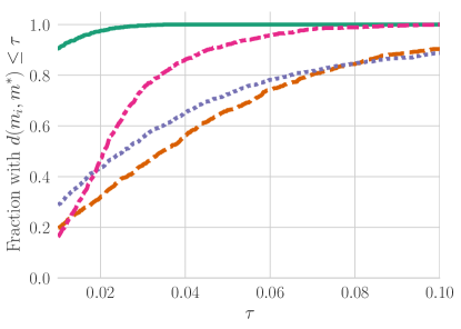
(a) High SNR, decay

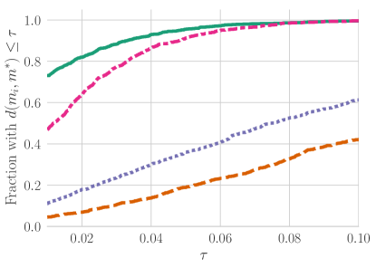
(b) Low SNR, decay

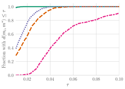
(c) High SNR, no decay

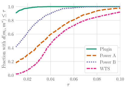
(d) Low SNR, no decay

Figure 1: Performance profiles for the plugin, power method A, power method B, and weighted Thompson Sampling estimators.

Table 1: Experiment Parameters

Type	Value
SNR $\frac{\|u\|_{2}}{\sigma}$	20 (high), 10 (low)
Experiment budget $N$	200
Plant length $r$	10
Input/output data length $r^{\prime}$	50
Plant decay $\rho$	0.75 (decay), 1.0 (no decay)
Number of random plants	100
Noise instances per plant	10

With this in mind, the performance profiles comparing the four algorithms are shown in Fig. 1. We see that for the plants with decaying impulse response coefficients, the plugin and WTS estimators are comparable. The latter estimator performs relatively worse in the experiments corresponding to no coefficient decay. As alluded to previously, this can most likely be attributed to our particular experimental setup: the WTS algorithm effectively grids the frequency response curve of the plant, and this set of plants allows for more relative variation in the curve than the onces with decaying coefficients.

6 Conclusion

We study lower bounds for $\mathcal{H}_{\infty}$-norm estimation for both passive and active algorithms. Our analysis shows that in the passive case model identification and $\mathcal{H}_{\infty}$-norm estimation have the same worst-case sample complexity. In the active setting, the lower bound improves by a factor that is logarithmic in the filter length. Experimentally, we see that the performance of a simple plugin $\mathcal{H}_{\infty}$-norm estimator is competitive with the proposed active algorithms for norm estimation in the literature.

Our work raises an interesting question as to whether there exists an active algorithm attaining the lower bound, or if instead the lower bound can be sharpened. In Section 3.2, we briefly discussed the technical hurdles that need to be overcome for both cases. Beyond resolving the gap between the lower bounds, an interesting question is how does the sample complexity of both model and norm estimation degrade when the filter length is unknown. Another direction is to extend the algorithms and analysis beyond single input single output (SISO) systems.

Appendix

Input: Normalized $u^{(1)}$.

for $t=1$ to $N$ do

       Perform the experiment $y^{(t)}=Gu^{(t)}+\eta^{(t)}$.

       Create the time-reversed $\tilde{y}^{(t)}$.

       $\mu^{(t)}=\|\tilde{y}^{(t)}\|_{2}$.

       $u^{(t+1)}=\tilde{y}^{(t)}/\mu^{(t)}$.

       $\hat{H}_{t}=\sqrt{\mu^{(t-1)}(u^{(t-1)})^{\top}\tilde{y}^{(t)}}.$

end for

return $\hat{H}_{N}$.

Algorithm 2 Power Method A [12]

Input: Normalized $u^{(1)}$.

for $t=1$ to $N/2$ do

       Perform the experiment $y^{(t)}=Gu^{(t)}+\eta^{(t)}$.

       Create the time-reversed $\tilde{y}^{(t)}$.

       Perform the experiment $z^{(t)}=G\tilde{y}^{(t)}+\eta^{\prime(t)}$.

       Create the time-reversed $\tilde{z}^{(t)}$.

       $\hat{H}_{t}=\sqrt{|(u^{(t)})^{\top}\tilde{z}^{(t)}}|$.

       $u^{(t+1)}=\tilde{z}^{(t)}/\|\tilde{z}^{(t)}\|_{2}$.

end for

return $\hat{H}_{(N/2)}$.

Algorithm 3 Power Method B [18]

Input: $M,\lambda,\sigma$, $\rho_{k}^{1}=1/K\;\forall\;k$, $m^{0}=0$, $v^{0}=\lambda^{2}I$.

for $t=1$ to $N$ do

       Input design: Create the normalized input signal $u^{(t)}$ proportional to the DFT power profile $p^{t}=\rho^{t}$.

       Perform the experiment $y^{(t)}=Gu^{(t)}+\eta^{(t)}$ and obtain DFT coefficients $X_{k}^{t}=Y_{k}^{t}/U_{k}^{t}$.

       Update the posterior for all $k$:

       $m_{k}^{t+1}=\frac{\lambda^{2}\sum_{\ell=1}^{t}p_{k}^{\ell}X_{k}^{\ell}}{\sigma^{2}+\lambda^{2}\sum_{\ell=1}^{t}p_{k}^{\ell}}$.

       $v_{k}^{t+1}=\lambda^{2}/(1+\lambda^{2}/\sigma^{2}\sum_{\ell=1}^{t}p_{k}^{\ell})$.

       Update the posterior $\rho^{t+1}$:

       Draw $s^{l}\sim\mathcal{N_{C}}(m_{k}^{t+1},v_{k}^{t+1}),\quad l=1,\ldots,M$.

       $\rho_{k}^{t+1}=\frac{1}{M}\sum_{l=1}^{M}\#(\operatorname*{arg\!\max}_{i}\{|s_{i}^{l}|\}=k)$.

       $\hat{H}_{t}=\max_{k}\sum_{\ell=1}^{t}p_{k}^{\ell}X_{k}^{\ell}/\sum_{\ell=1}^{t}p_{k}^{\ell}$.

end for

return $\hat{H}_{N}$.

Algorithm 4 Weighted Thompson Sampling (WTS) [9]

References

• [1] J.-Y. Audibert and S. Bubeck. Minimax policies for adversarial and stochastic bandits. In Conference on Learning Theory, 2009.
• [2] A. Böttcher and S. M. Grudsky. Toeplitz Matrices, Asymptotic Linear Algebra, and Functional Analysis. 2000.
• [3] S. Bubeck and N. Cesa-Bianchi. Regret analysis of stochastic and nonstochastic multi-armed bandit problems. Foundations and Trends® in Machine Learning, 5(1):1–122, 2012.
• [4] E. Dolan and J. Moré. Benchmarking optimization software with performance profiles. Mathematical Programming, 91(2):201–213, 2002.
• [5] A. Goldenshluger. Nonparametric Estimation of Transfer Functions: Rates of Convergence and Adaptation. IEEE Transactions on Information Theory, 44(2):644–658, 1998.
• [6] S. Gupta and S. M. Joshi. Some properties and stability results for sector-bounded lti systems. In 1994 IEEE 33rd Annual Conference on Conference on Decision and Control, 1994.
• [7] A. J. Helmicki, C. A. Jacobson, and C. N. Nett. Control oriented system identification: A worst-case/deterministic approach in $h_{\infty}$. IEEE Transactions on Automatic Control, 36(10):1163–1176, 1991.
• [8] E. Jonas, Q. Pu, S. Venkataraman, I. Stoica, and B. Recht. Occupy the cloud: Distributed computing for the 99%. In Proceedings of the 2017 Symposium on Cloud Computing, 2017.
• [9] M. I. Müller, P. E. Valenzuela, A. Proutiere, and C. R. Rojas. A stochastic multi-armed bandit approach to nonparametric $\mathcal{H}_{\infty}$-norm estimation. In 2017 IEEE 56th Annual Conference on Conference on Decision and Control, 2017.
• [10] T. Oomen, R. van der Maas, C. R. Rojas, and H. Hjalmarsson. Iterative data-driven $\mathcal{H}_{\infty}$ norm estimation of multivariable systems with application to robust active vibration isolation. IEEE Transactions on Control Systems Technology, 22(6):2247–2260, 2014.
• [11] G. Rallo, S. Formentin, C. R. Rojas, T. Oomen, and S. M. Savaresi. Data-driven $\mathcal{H}_{\infty}$-norm estimation via expert advice. In 2017 IEEE 56th Annual Conference on Conference on Decision and Control, 2017.
• [12] C. R. Rojas, T. Oomen, H. Hjalmarsson, and B. Wahlberg. Analyzing iterations in identification with application to nonparametric $\mathcal{H}_{\infty}$-norm estimation. Automatica, 48(11):2776–2790, 2012.
• [13] A. B. Tsybakov. Introduction to Nonparametric Estimation. 2009.
• [14] S. Tu, R. Boczar, A. Packard, and B. Recht. Non-asymptotic analysis of robust control from coarse-grained identification. arXiv, 2017. math.OC:1707.04791.
• [15] S. Tu, R. Boczar, and B. Recht. On the approximation of toeplitz operators for nonparametric $\mathcal{H}_{\infty}$-norm estimation. In 2018 Annual American Control Conference (ACC), 2018.
• [16] K. van Heusden, A. Karimi, and D. Bonvin. Data-driven estimation of the infinity norm of a dynamical system. In 2007 IEEE 46th Annual Conference on Conference on Decision and Control, 2007.
• [17] R. Vershynin. High-Dimensional Probability: An Introduction with Applications in Data Science. 2018.
• [18] B. Wahlberg, M. B. Syberg, and H. Hjalmarsson. Non-parametric methods for $\mathcal{L}_{2}$-gain estimation using iterative experiments. Automatica, 46(8):1376–1381, 2010.
• [19] Y. Wu. Lecture notes for ece598yw: Information-theoretic methods for high-dimensional statistics. http://www.stat.yale.edu/~yw562/teaching/598/ref.html, 2017.