DYNAMICAL COMPUTATION OF THE DENSITY OF STATES AND BAYES FACTORS
USING NONEQUILIBRIUM IMPORTANCE SAMPLING

Abstract.

Nonequilibrium sampling is potentially much more versatile than its equilibrium counterpart, but it comes with challenges because the invariant distribution is not typically known when the dynamics breaks detailed balance. Here, we derive a generic importance sampling technique that leverages the statistical power of configurations transported by nonequilibrium trajectories, and can be used to compute averages with respect to arbitrary target distributions. As a dissipative reweighting scheme, the method can be viewed in relation to the annealed importance sampling (AIS) method and the related Jarzynski equality. Unlike AIS, our approach gives an unbiased estimator, with provably lower variance than directly estimating the average of an observable. We also establish a direct relation between a dynamical quantity, the dissipation, and the volume of phase space, from which we can compute quantities such as the density of states and Bayes factors. We illustrate the properties of estimators relying on this sampling technique in the context of density of state calculations, showing that it scales favorable with dimensionality—in particular, we show that it can be used to compute the phase diagram of the mean-field Ising model from a single nonequilibrium trajectory. We also demonstrate the robustness and efficiency of the approach with an application to a Bayesian model comparison problem of the type encountered in astrophysics and machine learning.

1. Introduction

Statistical estimation using averages over a dynamical process typically relies on the principle of detailed balance. Consider a dynamical system

(1.1) $$\dot{\boldsymbol{X}}(t,\boldsymbol{x})=\boldsymbol{b}({\boldsymbol{X}}(t,\boldsymbol{x}))\qquad\boldsymbol{X}(0,\boldsymbol{x})=\boldsymbol{x}$$

where $\boldsymbol{x}\in\Omega\subset\mathbb{R}^{n}$ is a state that is propagated in time to ${\boldsymbol{X}}(t,\boldsymbol{x})$ via the vector field $\boldsymbol{b}:\Omega\to\mathbb{R}^{n}$. If the dynamics is microscopically reversible with respect to some target density $\rho(\boldsymbol{x})$, then this density is preserved under time evolution. Practically, this means that the expectation of an observable $\phi(\boldsymbol{x})$ with respect to $\rho(\boldsymbol{x})$, which we denote by $\langle\phi\rangle$, can be computed as a time average along an equilibrium trajectory generated from (1.1), provided that the dynamics is ergodic. This direct sampling scheme becomes inefficient if the expectation $\langle\phi\rangle$ is dominated by values of $\boldsymbol{x}$ that are rare under $\rho(\boldsymbol{x})$ and therefore infrequently visited by the dynamics (1.1).

Importance sampling estimates relying on nonequilibrium dynamics have shown success in a variety of applications, from statistical physics to machine learning [16, 15, 27, 3, 9, 22, 23]. Here, we derive a class of estimators based on an exact reweighting of the samples gathered during a nonequilibrium process with a stationary density. Similar to the annealed importance sampling (AIS) method [22] and estimators based on the Jarzynski equality [16], our scheme accelerates the transport of density to rare regions of phase space which may make substantial contributions to equilibrium averages. This basic idea is exploited by many different enhanced sampling techniques [1, 6, 25, 21]. Physically, the statistical weight of the transported density can be interpreted through the fluctuation theorem as a dissipative reweighting whose value can be derived explicitly. As we show, the resulting estimator is unbiased, unlike the AIS estimator, which requires computing a ratio of sample means (cf. Eq. (12) of Ref. [22]). Our estimator always has lower variance than the direct estimator, a reduction that comes at the nontrivial cost of generating trajectories. That said, nonequilibrium transport enables us to access states that are exponentially rare in original density but which may dominate expectation values; direct sampling fails dramatically in such settings.

2. Nonequilibrium estimators

A generic importance sampling scheme to compute the average with respect to some target density $\rho(\boldsymbol{x})$ reweights samples drawn from another density $\rho_{\text{ne}}(\boldsymbol{x})$

(2.1) $$\langle\phi\rangle=\langle\phi\rho/\rho_{\text{ne}}\rangle_{\text{ne}}.$$

Our samplers use for $\rho_{\text{ne}}(\boldsymbol{x})$ the non-equilibrium stationary density of a dynamical system based on generating trajectories by an initiate-then-propagate procedure: We draw points $\boldsymbol{x}$ from the density $\rho(\boldsymbol{x})$ that we then propagate forward and backward in time using the dynamics (1.1) until the trajectories $\boldsymbol{X}(t,\boldsymbol{x})$ hit some fixed target set. Concrete applications determine the appropriate choice of target sets: they could for example be the boundary of $\Omega$ or the fixed points of (1.1) in $\Omega$ . Using the set of trajectories generated this way we define the nonequilibrium average $\langle\cdot\rangle_{\text{ne}}$ as

(2.2) $$\langle\phi\rangle_{\text{ne}} =\frac{1}{\langle\tau\rangle}\int_{\Omega}\int_{\tau^{-}(\boldsymbol{x})}^{\tau^{+}(\boldsymbol{x})}\phi(\boldsymbol{X}(t,\boldsymbol{x}))dt\,\rho(\boldsymbol{x})d\boldsymbol{x}$$

where $\tau^{+}(\boldsymbol{x})\geq 0$ and $\tau^{-}(\boldsymbol{x})\leq 0$ are the first times at which $\boldsymbol{X}(t,\boldsymbol{x})\in\partial\Omega$ in the future or in the past, respectively, and $\langle\tau\rangle=\langle\tau^{+}\rangle-\langle\tau^{-}\rangle$. By changing integration variables using $X(t,\boldsymbol{x})\to\boldsymbol{x}$ and $t\to-t$ we can express (2.2) as

(2.3) $$\langle\phi\rangle_{\text{ne}}=\frac{1}{\langle\tau\rangle}\int_{\Omega}\phi(\boldsymbol{x})\int_{\tau^{-}(\boldsymbol{x})}^{\tau^{+}(\boldsymbol{x})}\!\!\!J(t,\boldsymbol{x})\rho(\boldsymbol{X}(t,\boldsymbol{x}))dt\,d\boldsymbol{x}$$

where $J(t,\boldsymbol{x})$ is the Jacobian of the transformation:

(2.4) $$J(t,\boldsymbol{x})=\exp\left({\textstyle\int_{0}^{t}\nabla\cdot\boldsymbol{b}(\boldsymbol{X}(s,\boldsymbol{x}))ds}\right).$$

Physically, the Jacobian corresponds to the total energy dissipation up to time $t$ along the trajectory. This derivation is described in detail in Appendix A). Now, (2.3) can be interpreted as an expectation with respect to a nonequilibrium density, $\langle\phi\rangle_{\text{ne}}=\int_{\Omega}\phi(\boldsymbol{x})\rho_{\text{ne}}(\boldsymbol{x})d\boldsymbol{x}$, with $\rho_{\text{ne}}(\boldsymbol{x})$ given by

(2.5) $$\rho_{\text{ne}}(\boldsymbol{x})=\frac{1}{\langle\tau\rangle}\int_{\tau^{-}(\boldsymbol{x})}^{\tau^{+}(\boldsymbol{x})}J(t,\boldsymbol{x})\rho(\boldsymbol{X}(t,\boldsymbol{x}))dt.$$

We can now use this expression for $\rho_{\text{ne}}(\boldsymbol{x})$ in (2.1) for reweighting. As shown in Appendix B this gives 

(2.6) $$\langle\phi\rangle=\left\langle\frac{\int_{\tau^{-}}^{\tau^{+}}\phi(\boldsymbol{X}(t))J(t)\rho(\boldsymbol{X}(t))dt}{\int_{\tau^{-}}^{\tau^{+}}J(t)\rho(\boldsymbol{X}(t))dt}\right\rangle$$

which yields the estimator, one of our main results,

(2.7) $$\langle\phi\rangle=\lim_{N\to\infty}\langle\phi\rangle_{N}\quad\text{where}\quad\langle\phi\rangle_{N}=\frac{1}{N}\sum_{i=1}^{N}\frac{\int_{\tau^{-}(\boldsymbol{x}_{i})}^{\tau^{+}(\boldsymbol{x}_{i})}\phi(\boldsymbol{X}(t,\boldsymbol{x}_{i}))J(t,\boldsymbol{x}_{i})\rho(\boldsymbol{X}(t,\boldsymbol{x}_{i}))dt}{\int_{\tau^{-}(\boldsymbol{x}_{i})}^{\tau^{+}(\boldsymbol{x}_{i})}J(t,\boldsymbol{x}_{i})\rho(\boldsymbol{X}(t,\boldsymbol{x}_{i}))dt},$$

provided that the points $\boldsymbol{x}_{i}$ are drawn (not necessarily independently) from $\rho(\boldsymbol{x})$. An equivalent to (2.6) using no target set and running the trajectories on a finite time lag instead is given in Appendix C. The estimator (2.6)reweights points sampled along a nonequilibrium trajectory according to their dissipation, a physically analogous strategy to that in AIS (see Appendix E for a more detailed comparison with AIS).

Unlike other dissipative reweighting strategies, the estimator $\langle\phi\rangle_{N}$ is unbiased, valid for any dynamics (1.1) and any target density $\rho(\boldsymbol{x})$. Like standard Metropolis Monte-Carlo, it only requires knowing the density up to a normalization factor. It has lower variance than the direct estimator $N^{-1}\sum_{i=1}^{N}\phi(\boldsymbol{x}_{i})$   since the variance of this direct estimator is $N^{-1}(\langle\phi^{2}\rangle-\langle\phi\rangle^{2})$ whereas the variance of $\langle\phi\rangle_{N}$ is $N^{-1}(A-\langle\phi\rangle^{2})$ with $A\leq\langle\phi^{2}\rangle$ since Jensen’s inequality implies

(2.8) $$A=\left\langle\Bigg{|}\frac{\int_{\tau^{-}}^{\tau^{+}}\phi(\boldsymbol{X}(t))J(t)\rho(\boldsymbol{X}(t))dt}{\int_{\tau^{-}}^{\tau^{+}}J(t)\rho(\boldsymbol{X}(t))dt}\Bigg{|}^{2}\right\rangle\leq\left\langle\frac{\int_{\tau^{-}}^{\tau^{+}}|\phi(\boldsymbol{X}(t))|^{2}J(t)\rho(\boldsymbol{X}(t))dt}{\int_{\tau^{-}}^{\tau^{+}}J(t)\rho(\boldsymbol{X}(t))dt}\right\rangle=\left\langle\phi^{2}\right\rangle.$$

With a proper choice of $\boldsymbol{b}(\boldsymbol{x})$ the estimator $\langle\phi\rangle_{N}$ in (2.7) has the potential to significantly outperform the direct estimator (in Appendix D we show that $\langle\phi\rangle_{N}$ is a zro-variance estimator in one-dimension). It does so by transporting points drawn naively from $\rho(\boldsymbol{x})$ towards regions that statistically dominate the expectation of $\phi(\boldsymbol{x})$. In practice, it is also simple to use: (i) sample points $\boldsymbol{x}_{i}$ from $\rho(\boldsymbol{x})$ using e.g. standard Monte Carlo; (ii) compute the trajectory $\boldsymbol{X}(t,\boldsymbol{x}_{i})$ passing through each of these points by integrating (1.1) forward and backward in time until $\boldsymbol{X}(\tau^{\pm}(\boldsymbol{x}_{i}),\boldsymbol{x}_{i})\in\partial\Omega$ (which also gives $\tau^{\pm}(\boldsymbol{x}_{i})$); (iii) use these data to calculate $J(t,\boldsymbol{x}_{i})$ from (2.4) first, then the integrals in (2.7); (iv) average the results to get $\langle\phi\rangle_{N}$. Note that the operations in (ii) and (iii) can be performed in parallel, and we can monitor the value of the running average $\langle\phi\rangle_{N}$ as $N$ increases to check convergence.

Let us also note that a discrete-time equivalent of 2.6 has now been given in [28].

3. Density of states (DOS)

Consider a $d$-dimensional system with position $\boldsymbol{q}\in\mathbb{R}^{d}$, momenta $\boldsymbol{p}\in\mathbb{R}^{d}$, and Hamiltonian $\mathcal{H}(\boldsymbol{q},\boldsymbol{p})=\tfrac{1}{2}|\boldsymbol{p}|^{2}+U(\boldsymbol{q})$ where $U(\boldsymbol{q})$ is some potential bounded from below. Let $V(E)$ be the volume of phase space below some threshold energy $E$,

(3.1) $$V(E)=\int_{\mathcal{H}(\boldsymbol{q},\boldsymbol{p})<E}\ d\boldsymbol{q}d\boldsymbol{p},$$

From $V(E)$ one can compute the DOS, $D(E)=V^{\prime}(E)$, or the canonical partition function, $Z(\beta)=\int_{\mathbb{R}}e^{-\beta E}D(E)dE=\beta\int_{\mathbb{R}}e^{-\beta E}V(E)dE$.

To calculate (3.1) with our estimator (2.7), we set $\boldsymbol{x}=(\boldsymbol{q},\boldsymbol{p})$, define $\Omega=\{(\boldsymbol{q},\boldsymbol{p}):\mathcal{H}(\boldsymbol{q},\boldsymbol{p})<E_{\max}\}$ for some $E_{\max}<\infty$, and use dissipative Langevin dynamics with $\boldsymbol{b}(\boldsymbol{x})=(\boldsymbol{p},-\nabla U(\boldsymbol{q})-\gamma\boldsymbol{p})$ in (1.1)

(3.2) $$\dot{\boldsymbol{q}}=\boldsymbol{p},\qquad\dot{\boldsymbol{p}}=-\nabla U(\boldsymbol{q})-\gamma\boldsymbol{p},$$

for some friction coefficient $\gamma>0$. With this choice, the dissipative term in the estimator (2.7) takes the simple form:

(3.3) $$J(t,\boldsymbol{x})=e^{-d\gamma t}.$$

If we also choose the target density $\rho(\boldsymbol{x})$ to be uniform in $\Omega$, the estimator further simplifies due to cancelation of the two $\rho$ terms in (2.7). We arrive at

(3.4) $$\frac{V(E)}{V(E_{\text{max}})}=\lim_{N\to\infty}\frac{1}{N}\sum_{i=1}^{N}e^{-d\gamma\left(\tau^{E}(\boldsymbol{x}_{i})-\tau^{-}(\boldsymbol{x}_{i})\right)}$$

where $\tau^{E}(\boldsymbol{x})$ denotes the positive (and possibly infinite) or negative time for a trajectory initiated from $\boldsymbol{x}=(\boldsymbol{q},\boldsymbol{p})$ to reach energy $E\leq E_{\text{max}}$ under the dynamics (3.2). Eq. (3.4) is our second main result: it establishes a dictionary between a nonequilibrium dynamical quantity and a purely static, global property of the energy landscape, $V(E)$. This result asserts that the rate of decrease of the volume of phase space can be measured by computing an average of the total dissipation of nonequilibrium descent trajectories. We do not know of an analogous result in the literature.

The $\tau^{+}(\boldsymbol{x})$ terms vanish in this dynamics because the time to reach a local minimum diverges . In practice we halt the forward trajectories when the norm of the gradient is below some tolerance. To compute an unnormalized volume, we can estimate $V(E_{\text{max}})$ with standard Monte Carlo integration.

The power of the procedure we have described comes from the fact that the forward trajectories are guaranteed to visit regions of low energy around local minima of $U(\boldsymbol{q})$ that would otherwise be difficult to sample by drawing points uniformly in $\{\mathcal{H}(\boldsymbol{q},\boldsymbol{p})<E_{\max}\}$. In this regard our approach is also similar to nested sampling [26, 7, 24, 19, 5]. Like nested sampling, we do not require an a priori stratification of the energy shells, which is the way the DOS is typically calculated via thermodynamic integration [12, 13] or simulated tempering [17, 10]. Our method also offers several advantages over nested sampling. First, the depth of energies reached in nested sampling is determined by the initial number of points used in a computation. If too few points are used, the calculation must be repeated in full with a larger number of initial points. Here, the accuracy of the calculation improves and explores deeper minima simply by running additional ascent/descent trajectories. In addition, our approach does not require uniform sampling below every energy level, which is required in nested sampling and is a difficult condition to implement [19]. We must only generate points uniformly below the highest energy level, $E_{\max}$, which is usually much easier. Computationally, we also benefit from the fact that every trajectory contributes independently to our estimator, meaning that the implementation is trivially parallelizable.

4. Variance estimation in the small $\gamma$ limit

We know from (2.8) that the variance of our estimator is lower than that of the direct estimator. In the specific context of a DOS calculation using (3.2), we can analyze the variance more explicitly in the limit of small $\gamma$, in which the descent dynamics in (3.2) reduces to a closed equation for the energy $E=\mathcal{H}(\boldsymbol{q},\boldsymbol{p})$ on the rescaled time $t^{\prime}=\gamma t$. This dynamics evolves on the disconnectivity (or Reeb) graph [29], which branches at every energy level at which a basin where $\mathcal{H}(\boldsymbol{q},\boldsymbol{p})\leq E$ splits into more than one connected component. In the simplest case when the potential $U(\boldsymbol{q})$ has a single well, the graph has only one branch and the value of $\gamma(\tau^{E}(\boldsymbol{x}_{i})-\tau^{-}(\boldsymbol{x}_{i}))$ becomes the same along every trajectory when $\gamma\to 0$. Therefore the estimator (3.4) has zero variance—a single trajectory gives the exact value for $V(E)/V(E_{\text{max}})$. If the disconnectivity graph has several branches, we can count all the paths along the graph starting at $E=E_{\text{max}}$ which end at a given branch. Assuming that the number of such paths is $M\geq 1$, we can associate a deterministic time $\Delta\tau^{E}_{j}>0$, possibly infinite, along each path. We define $\Delta\tau^{E}_{j}$ with $j=1,\ldots,M$ as the total rescaled time the trajectory takes to go from $\mathcal{H}(\boldsymbol{q},\boldsymbol{p})=E_{\text{max}}$ to $\mathcal{H}(\boldsymbol{q},\boldsymbol{p})=E$ by the effective dynamics for $E$ along the path with index $j$ and $\Delta\tau^{E}_{j}=\infty$ if the path terminates at an energy $E^{\prime}>E$. For any initial condition, $\lim_{\gamma\to 0}\gamma(\tau^{E}(\boldsymbol{x}_{i})-\tau^{-}(\boldsymbol{x}_{i}))=\Delta\tau^{E}_{j}$ for some index $j$, meaning the only random component in the procedure is which path is picked if the trajectory starts at $\boldsymbol{x}_{i}$. We denote by $p_{j}$ the probability, computed over all initial conditions drawn uniformly in $\{\mathcal{H}(\boldsymbol{q},\boldsymbol{p})<E_{\max}\}$, that the path with index $j$ is taken. Then in the small $\gamma$ limit the mean and variance of the estimator (3.4) are

(4.1) mean $$=\frac{V(E)}{V(E_{\text{max}})}=\sum_{j=1}^{M}p_{j}e^{-d\Delta\tau^{E}_{j}},$$

variance $$=\sum_{j=1}^{M}p_{j}e^{-2d\Delta\tau^{E}_{j}}-\text{mean}^{2}.$$

The specific values of $p_{j}$, $\Delta\tau_{j}^{E}$, and $M$ which determine the quality of the estimator (3.4) depend on both the structure of the disconnectivity graph and the effective equation for the energy on this graph. What is remarkable, however, is that $p_{j}$, $\Delta\tau_{j}^{E}$, and $M$ depend on the dimensionality of the system only indirectly. In high dimensional settings, the complexity of the disconnectivity is a generic challenge, but our approach has favorable properties even in these difficult cases. In particular, the computational cost of the procedure increases only linearly in $\gamma$ as we decrease this parameter to small values. We also stress that the formulae (4.1) for the mean and variance rely on the assumption $\gamma\ll 1$, but the estimator remains valid for any value of $\gamma.$

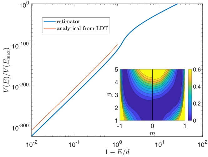
Figure 1. Mean-field Ising model with potential (5.1): volume ratio obtained from (3.4) using a single ascent / descent trajectory. The inset shows the free energy in $\beta$ and $m=d^{-1}\sum_{i=1}^{d}\cos(q_{i})$ that can also be estimated from this single trajectory (right half) and analytically using large deviation theory (left half).

5. Phase diagram of the mean-field Ising model.

As an illustration of the statistical power contained in the nonequilibrium trajectories, we computed the phase diagram of the mean-field Ising model with potential

(5.1) $$U(\boldsymbol{q})=-\frac{1}{2d}\sum_{i,j=1}^{d}\cos(q_{i})\cos(q_{j}).$$

This system is known to display a phase transition in temperature at the critical $\beta_{c}=2$ [20]. The potential (5.1) is double-well, but because of the symmetry $\boldsymbol{q}\to-\boldsymbol{q}$ a single ascent / descent trajectory can be used to estimate the volume ratio $V(E)/V(E_{\text{max}})$. We note that while there are only to energy minima, the energy landscape has an exponential number of critical points (the derivative with respect to $\theta_{j}$ vanishes $2^{d}$ when $\sin(\theta_{j})=0$), so the geometry of the landscape is nontrivial. We performed this calculation when $d=100$ with $\gamma=10^{-3}$ to obtain the result shown in Fig. 1: as can be seen, this result spans 300 order of magnitudes and compares very well with the analytical estimate that can be obtained in the large $d$ limit, as described in Appendix F. The single ascent /descent trajectory can also be used to calculate the free energy in $\beta$ and magnetization $m=d^{-1}\sum_{i=1}^{d}\cos(q_{i})$ of the system (see Appendix F for details). The result shown in the inset of Fig. 1 demonstrates that our estimate compares well with the large $d$ estimate. The code to reproduce these experiments is available on Gitlab . The numerical experiments require only several minutes of computation on a single core, but parallelization strategies could dramatically reduce the duration.

6. Bayes factors

The computations for the density of states have an equivalent manifestation in Bayesian estimation. Given a model $\mathcal{M}$, one seeks to maximize the probability of a set of parameters $\theta\in\mathbb{R}^{d}$ conditioned on observations of data $\mathcal{D}.$ Using Bayes Theorem, we can write

(6.1) $$\mathbb{P}(\boldsymbol{\theta}|\mathcal{D},\mathcal{M})=\mathcal{L}(\boldsymbol{\theta})\pi(\boldsymbol{\theta})/Z$$

where $\mathcal{L}(\boldsymbol{\theta})=\mathbb{P}(\mathcal{D}|\boldsymbol{\theta},\mathcal{M})$ is the likelihood function, $\pi(\boldsymbol{\theta})=\mathbb{P}(\boldsymbol{\theta}|\mathcal{M})$ is the prior, and $Z=\mathbb{P}(\mathcal{D}|\mathcal{M})=\int\mathcal{L}(\boldsymbol{\theta})\pi(\boldsymbol{\theta})d\boldsymbol{\theta}$ is the partition function, often called the Bayesian evidence in this context; it is the canonical partition function with $\beta=1.$

In Bayesian inference, we choose a model and then estimate its parameters without knowledge of the partition function by doing gradient descent on $-\log\mathcal{L}(\boldsymbol{\theta})\equiv U(\boldsymbol{\theta}),$ which depends on the model we have taken. However, there is no a priori guarantee that the chosen model is optimal, so it is often necessary to make comparisons of two distinct models $\mathcal{M}$ and $\mathcal{M^{\prime}}$. Ideally, one would compare the probability of the observed data given each model, that is the Bayes factors

(6.2) $$Z/Z^{\prime}=\mathbb{P}(\mathcal{D}|\mathcal{M})/\mathbb{P}(\mathcal{D}|\mathcal{M}^{\prime}).$$

Similarly, computing posterior probabilities also requires knowledge of the partition function.

As we have already emphasized, computing $Z$ is intractable analytically in all but the simplest cases. [26] demonstrated that it is possible to numerically evaluate the “prior volume”,

(6.3) $$V(L)=\int_{\mathcal{L}(\boldsymbol{\theta})\geq L}\pi(\boldsymbol{\theta})d\boldsymbol{\theta}$$

to produce an estimate of $Z$ via

(6.4) $$Z=\int_{0}^{L_{0}}V(L)\ dL,$$

where $L_{0}$ is the maximum value of the likelihood. Just as in the density of states calculation, we can evaluate the Bayesian evidence by using trajectorial estimators.

To do so, we sample parameters of the model $\mathcal{M}$ uniformly and define a flow of parameters via dissipative Langevin dynamics with $U(\boldsymbol{\theta})=-\log\mathcal{L}(\boldsymbol{\theta})$ (which also gives $L_{0}$ from the terminal point of the descent trajectories). We construct an estimate of $Z$ by computing $V(L)$ using Eq. (3.4) and numerically integrating Eq. (6.4) using quadrature. Note that the contribution from the momenta can be factored out and the resulting Gaussian integral can be computed exactly.

Figure 2. Mixture of Gaussians inference problem with $d=10$ and 50 wells in the mixture. The volume of states below $E=-\log{\mathcal{L}}$ is shown as red circles. In the small gamma limit, the time to reach energy $E$, $\Delta\tau=\tau^{E}-\tau^{-}$, should be independent of the initial condition. The inset shows that the dissipative dynamics converges to many different local minima, corresponding to the individually discernible lines in the inset. A total of $N=100$ trajectories are plotted, but there are fewer than one hundred visible lines, meaning that some trajectories not only end in the same basin, but also have decay in energy at the same rate, as the small $\gamma$ limit predicts. This demonstrates that the low variance regime can be achieved even with modest values of $\gamma.$

We tested our approach using a mixture of Gaussians model, a benchmark which has been used to characterize nested sampling for inference problems [11]. The model is defined as a mixture of $n$ distributions in dimension $d$ with amplitudes $A_{i}$,

(6.5) $$\mathcal{L}(\boldsymbol{\theta})=\sum_{i=1}^{n}A_{i}e^{-\tfrac{1}{2}(\boldsymbol{\theta}-\boldsymbol{\mu}_{i})^{T}\boldsymbol{\Sigma}_{i}^{-1}(\boldsymbol{\theta}-\boldsymbol{\mu}_{i})}.$$

Though we do not have access to the exact expression for $V(E)$ at all energy levels in this model, we can evaluate the partition function $Z$ exactly.

We used $n=50$ wells with depths exponentially distributed in dimension $d=10$, an example much more complex than previous benchmarks. While this landscape is not rugged, in mixture of Gaussian problems entropic effects can lead to extremely difficult optimization problems because we are required to sample exponentially small volumes. In this regime, brute force Monte Carlo approaches fail dramatically. Fig. 2 illustrates the statistical power of the trajectory reweighting approach. With only 100 trajectories, we recover the volume of states for the likelihood function extremely accurately, especially at low energies, where the standard error is vanishingly small. An accurate estimate at low energies leads to robust estimates of $Z$ because the contribution to $Z$ decays exponentially with $E$. In particular, we know the low energy volume estimates are accurate because we compute $Z=17.41$ versus the exact result $Z=17.10$. For this calculation we set $E_{\text{max}}=450$, meaning that the states we neglected have likelihood lower than $e^{-450}$.

7. Conclusions

Any estimate of the microcanonical partition function requires a thorough exploration of the states of the system. Both naive Monte Carlo sampling and equilibrium dynamics often fail to visit states, which, though rare, dramatically impact the thermodynamic properties of the system. A nonequilibrium dynamics suffers from precisely the opposite problem: it explores the states rapidly, but not in proportion to their equilibrium probabilities. Our estimator, via Eq. (3.4) establishes a simple link between a nonequilibrium dynamical observable and a static property, the volume of phase space.

With a properly formulated algorithm, we can fully account for the statistical bias of a nonequilibrium dynamics. The resulting estimators can access states that are extremely atypical in equilibrium sampling schemes, but nevertheless physically consequential. While we demonstrated the potential of these estimators by computing the density of states and the computationally analogous Bayes factor, the expression in (2.7) is extremely general. Attractive applications within reach include adapting this approach to basin volume calculations [2, 18], computing the partition function of restricted Boltzmann machines [22, 14], and importance sampling to compute properties of systems in nonequilibrium stationary states, like active matter [4, 8].

Appendix A Derivation of expression (2.5) for $\rho_{\text{ne}}(\boldsymbol{x})$

To derive the expression in (2.5) for the density $\rho_{\text{ne}}(\boldsymbol{x})$, consider first the forward time trajectories alone and let us define the forward density $\rho_{\text{ne}}^{+}(\boldsymbol{x})$ via

(A.1) $$\langle\phi\rangle^{+}_{{\rm ne}} =\frac{1}{\langle\tau^{+}\rangle}\int_{\Omega}\int_{0}^{\tau^{+}(\boldsymbol{x})}\phi(\boldsymbol{X}(t,\boldsymbol{x}))dt\,\rho(\boldsymbol{x})d\boldsymbol{x}$$

$$\equiv\int_{\Omega}\phi(\boldsymbol{x})\rho^{+}_{\text{ne}}(\boldsymbol{x})d\boldsymbol{x}$$

The nonequilibrium density $\rho_{\text{ne}}^{+}(\boldsymbol{x})$ satisfies the stationary Liouville equation

(A.2) $$\langle\tau^{+}\rangle^{-1}\rho(\boldsymbol{x})=\nabla\cdot\left(\boldsymbol{b}(\boldsymbol{x})\rho^{+}_{\rm ne}(\boldsymbol{x})\right),$$

with the boundary condition $\rho^{+}_{\rm ne}(\boldsymbol{x})=0$ on the regions of $\partial\Omega$ where $\boldsymbol{b}(\boldsymbol{x})$ points inward (since, by construction, no mass can be transported there forward in time). Physically, this equation asserts that, at stationarity, the nonequilibrium probability flux out of a small volume in the vicinity of $\boldsymbol{x}$ is balanced by the rate of reinjection. To solve (A.2) notice that if we differentiate $\rho_{\rm ne}^{+}(\boldsymbol{X}(t,\boldsymbol{x}))$ with respect to time, by the chain rule we have

(A.3) $$\frac{d}{dt}\rho_{\rm ne}^{+}=\boldsymbol{b}\cdot\nabla\rho_{\rm ne}^{+}=\langle\tau^{+}\rangle^{-1}\rho-(\nabla\cdot\boldsymbol{b})\rho_{\rm ne}^{+}$$

where all functions are evaluated at $\boldsymbol{X}(t,\boldsymbol{x})$ and we used Eq. (1) for $\boldsymbol{X}(t,\boldsymbol{x})$ to derive the first equality and (A.2) to derive the second. Using the Jacobian (Eq. (5)),

(A.4) $$J(t,\boldsymbol{x})=\exp\left({\textstyle\int_{0}^{t}\nabla\cdot\boldsymbol{b}(\boldsymbol{X}(s,\boldsymbol{x}))ds}\right),$$

we can write (A.3) as

(A.5) $$\frac{d}{dt}\left(\rho_{\rm ne}^{+}(\boldsymbol{X}(t,\boldsymbol{x}))J(t,\boldsymbol{x})\right)=\langle\tau^{+}\rangle^{-1}\rho(\boldsymbol{X}(t,\boldsymbol{x}))J(t,\boldsymbol{x}).$$

Integration from $t=\tau^{-}(\boldsymbol{x})$ to $t=0$ using the boundary condition $\rho_{\rm ne}^{+}(\boldsymbol{X}(\tau^{-}(\boldsymbol{x}),\boldsymbol{x}))=0$ gives

(A.6) $$\rho_{\rm ne}^{+}(\boldsymbol{x})=\langle\tau^{+}\rangle^{-1}\int_{\tau^{-}(\boldsymbol{x})}^{0}J(t,\boldsymbol{x})\rho(\boldsymbol{X}(t,\boldsymbol{x}))dt.$$

A similar calculation gives the nonequilbrium stationary density resulting from the reverse time propagation of the dynamics, $\rho_{\rm ne}^{-}(\boldsymbol{x})$, defined via

(A.7) $$\langle\phi\rangle^{-}_{\rm ne} =\frac{1}{\langle\tau^{-}\rangle}\int_{\Omega}\int^{0}_{\tau^{-}(\boldsymbol{x})}\phi(\boldsymbol{X}(t,\boldsymbol{x}))dt\,\rho(\boldsymbol{x})d\boldsymbol{x}$$

$$\equiv\int_{\Omega}\phi(\boldsymbol{x})\rho^{-}_{\text{ne}}(\boldsymbol{x})d\boldsymbol{x}$$

We obtain

(A.8) $$\rho_{\rm ne}^{-}(\boldsymbol{x})=\langle\tau^{-}\rangle^{-1}\int^{\tau^{+}(\boldsymbol{x})}_{0}J(t,\boldsymbol{x})\rho(\boldsymbol{X}(t,\boldsymbol{x}))dt.$$

The nonequilibrium density defined via Eq. (4) can then be expressed by superposing $\rho_{\rm ne}^{+}(\boldsymbol{x})$ and $\rho_{\rm ne}^{-}(\boldsymbol{x})$:

(A.9) $$\rho_{\textrm{ne}}(\boldsymbol{x}) =\frac{\langle\tau^{+}\rangle\rho_{\rm ne}^{+}(\boldsymbol{x})-\langle\tau^{-}\rangle\rho_{\rm ne}^{-}(\boldsymbol{x})}{\langle\tau\rangle}$$

$$=\langle\tau\rangle^{-1}\int_{\tau^{-}(\boldsymbol{x})}^{\tau^{+}(\boldsymbol{x})}J(t,\boldsymbol{x})\rho(\boldsymbol{X}(t,\boldsymbol{x}))dt$$

This is (2.5)

Appendix B Derivation of expression (2.6) for the estimator

To derive the estimator in (2.6), start from (2.1) and write

(B.1) $$\langle\phi\rangle =\langle\phi\rho/\rho_{\text{ne}}\rangle_{\text{ne}}$$

$$=\frac{1}{\langle\tau\rangle}\int_{\mathbb{R}^{d}}\int_{\tau^{-}(\boldsymbol{x})}^{\tau^{+}(\boldsymbol{x})}\frac{\phi(\boldsymbol{X}(t,\boldsymbol{x}))\rho(\boldsymbol{X}(t,\boldsymbol{x}))}{\rho_{\text{ne}}(\boldsymbol{X}(t,\boldsymbol{x}))}dt\,\rho(\boldsymbol{x})d\boldsymbol{x}$$

$$=\int_{\mathbb{R}^{d}}\int_{\tau^{-}(\boldsymbol{x})}^{\tau^{+}(\boldsymbol{x})}\frac{\phi(\boldsymbol{X}(t,\boldsymbol{x}))\rho(\boldsymbol{X}(t,\boldsymbol{x}))}{\int_{\tau^{-}(\boldsymbol{X}(t,\boldsymbol{x}))}^{\tau^{+}(\boldsymbol{X}(t,\boldsymbol{x}))}J(s,\boldsymbol{X}(t,\boldsymbol{x}))\rho(\boldsymbol{X}(s,\boldsymbol{X}(t,\boldsymbol{x})))ds}dt\,\rho(\boldsymbol{x})d\boldsymbol{x}.$$

Using $\boldsymbol{X}(s,\boldsymbol{X}(t,\boldsymbol{x}))=\boldsymbol{X}(s+t,\boldsymbol{x})$ we have

(B.2) $$J(s,\boldsymbol{X}(t,\boldsymbol{x})) =\exp\left({\textstyle\int_{0}^{s}\nabla\cdot\boldsymbol{b}(\boldsymbol{X}(u,\boldsymbol{X}(t,\boldsymbol{x})))du}\right)$$

$$=\exp\left({\textstyle\int_{0}^{s}\nabla\cdot\boldsymbol{b}(\boldsymbol{X}(u+t,\boldsymbol{x}))du}\right)$$

$$=\exp\left({\textstyle\int_{t}^{s+t}\nabla\cdot\boldsymbol{b}(\boldsymbol{X}(u^{\prime},\boldsymbol{x}))du^{\prime}}\right)$$

$$=\frac{J(s+t,\boldsymbol{x})}{J(t,\boldsymbol{x})}$$

which implies that we can transform the denominator in (2.6) into

(B.3) $$\int_{\tau^{-}(\boldsymbol{X}(t,\boldsymbol{x}))}^{\tau^{+}(\boldsymbol{X}(t,\boldsymbol{x}))}J(s,\boldsymbol{X}(t,\boldsymbol{x}))\rho(\boldsymbol{X}(s,\boldsymbol{X}(t,\boldsymbol{x})))ds$$

$$= \frac{1}{J(t,\boldsymbol{x})}\int_{\tau^{-}(\boldsymbol{X}(t,\boldsymbol{x}))}^{\tau^{+}(\boldsymbol{X}(t,\boldsymbol{x}))}J(s+t,\boldsymbol{x})\rho(\boldsymbol{X}(s+t,\boldsymbol{x})))ds$$

$$= \frac{1}{J(t,\boldsymbol{x})}\int_{\tau^{-}(\boldsymbol{X}(t,\boldsymbol{x}))+t}^{\tau^{+}(\boldsymbol{X}(t,\boldsymbol{x}))+t}J(s^{\prime},\boldsymbol{x})\rho(\boldsymbol{X}(s^{\prime},\boldsymbol{x})))ds^{\prime}$$

$$= \frac{1}{J(t,\boldsymbol{x})}\int_{\tau^{-}(\boldsymbol{x})}^{\tau^{+}(\boldsymbol{x})}J(s^{\prime},\boldsymbol{x})\rho(\boldsymbol{X}(s^{\prime},\boldsymbol{x})))ds^{\prime}$$

Inserting this expression in (2.6) gives

(B.4) $$\langle\phi\rangle =\int_{\mathbb{R}^{d}}\int_{\tau^{-}(\boldsymbol{x})}^{\tau^{+}(\boldsymbol{x})}\frac{\phi(\boldsymbol{X}(t,\boldsymbol{x}))J(t,\boldsymbol{x})\rho(\boldsymbol{X}(t,\boldsymbol{x}))}{\int_{\tau^{-}(\boldsymbol{x})}^{\tau^{+}(\boldsymbol{x})}J(s^{\prime},\boldsymbol{x})\rho(\boldsymbol{X}(s^{\prime},\boldsymbol{x}))ds^{\prime}}dt\,\rho(\boldsymbol{x})d\boldsymbol{x}$$

$$=\int_{\mathbb{R}^{d}}\frac{\int_{\tau^{-}(\boldsymbol{x})}^{\tau^{+}(\boldsymbol{x})}\phi(\boldsymbol{X}(t,\boldsymbol{x}))J(t,\boldsymbol{x})\rho(\boldsymbol{X}(t,\boldsymbol{x}))dt}{\int_{\tau^{-}(\boldsymbol{x})}^{\tau^{+}(\boldsymbol{x})}J(t,\boldsymbol{x})\rho(\boldsymbol{X}(t,\boldsymbol{x}))dt}\,\rho(\boldsymbol{x})d\boldsymbol{x}$$

which is (2.6). Note that this equality holds even if $\tau_{-}(\boldsymbol{x})=-\infty$ and/or $\tau_{+}(\boldsymbol{x})=+\infty$, as long as the time integrals converge. That is, we don’t necessarily need to introduce target sets to make the descent / ascent trajectories finite.

Appendix C Fixed time equivalent of (2.6)

Suppose that $\boldsymbol{X}(t,\boldsymbol{x})\in\Omega$ for all $\boldsymbol{x}\in\Omega$ and $t\in\mathbb{R}$. Then, given any $-\infty\leq T_{1}<T_{2}\leq\infty$, we have the following estimator

(C.1) $$\langle\phi\rangle=\left\langle\int_{T_{-}}^{T_{+}}\frac{\phi(\boldsymbol{X}(t))\rho(\boldsymbol{X}(t))J(t)}{\int_{t-T_{+}}^{t-T_{-}}\rho(\boldsymbol{X}(s))J(s)ds}dt\right\rangle$$

For $T_{-}=-\infty$ and $T_{+}=\infty$, assuming that the integrals converge, this estimator can also be written as

(C.2) $$\langle\phi\rangle=\left\langle\frac{\int_{-\infty}^{\infty}\phi(\boldsymbol{X}(t))\rho(\boldsymbol{X}(t))J(t)dt}{\int_{-\infty}^{\infty}\rho(\boldsymbol{X}(t))J(t)dt}\right\rangle$$

This is the same as (2.6) when $\tau_{-}(\boldsymbol{x})=\-infty$ and $\tau_{+}(\boldsymbol{x})=+\infty$ for all $\boldsymbol{x}\in\Omega$.

To establish (F.16), notice that its left hand side is

(C.3) LHS(F.16) $$=\int_{\mathbb{R}^{n}}\int_{T_{-}}^{T_{+}}\frac{\phi(\boldsymbol{X}(t,\boldsymbol{x}))\rho(\boldsymbol{X}(t,\boldsymbol{x}))J(t,\boldsymbol{x})}{\int_{t-T_{+}}^{t-T_{-}}\rho(\boldsymbol{X}(s,\boldsymbol{x}))J(s,\boldsymbol{x})ds}dt\rho(\boldsymbol{x})d\boldsymbol{x}$$

$$=\int_{T_{-}}^{T_{+}}\int_{\mathbb{R}^{n}}\frac{\phi(\boldsymbol{X}(t,\boldsymbol{x}))\rho(\boldsymbol{X}(t,\boldsymbol{x}))J(t,\boldsymbol{x})}{\int_{t-T_{+}}^{t-T_{-}}\rho(\boldsymbol{X}(s,\boldsymbol{x}))J(s,\boldsymbol{x})ds}\rho(\boldsymbol{x})d\boldsymbol{x}dt$$

Now use $\boldsymbol{x}^{\prime}=\boldsymbol{X}(t,\boldsymbol{x})$ as new integration variable, the group property of the flow to set $\boldsymbol{x}=\boldsymbol{X}(-t,\boldsymbol{x}^{\prime})$ and $\boldsymbol{X}(s,\boldsymbol{x})=\boldsymbol{X}(s,\boldsymbol{X}(-t,\boldsymbol{x}^{\prime}))=\boldsymbol{X}(s-t,\boldsymbol{x}^{\prime})$, as well as $J(s,\boldsymbol{X}(-t,\boldsymbol{x}^{\prime}))=J(s-t,\boldsymbol{x}^{\prime})/J(-t,\boldsymbol{x}^{\prime})$ to obtain

(C.4) LHS(F.16) $$=\int_{T_{-}}^{T_{+}}\int_{\mathbb{R}^{n}}\frac{\phi(\boldsymbol{x}^{\prime})\rho(\boldsymbol{x}^{\prime})/J(-t,\boldsymbol{x}^{\prime})}{\int_{t-T_{+}}^{t-T_{-}}\rho(\boldsymbol{X}(s-t,\boldsymbol{x}^{\prime}))J(s-t,\boldsymbol{x}^{\prime})/J(-t,\boldsymbol{x}^{\prime})ds}\rho(\boldsymbol{X}(-t,\boldsymbol{x}^{\prime}))J(-t,\boldsymbol{x}^{\prime})d\boldsymbol{x}^{\prime}dt$$

$$=\int_{T_{-}}^{T_{+}}\int_{\mathbb{R}^{n}}\frac{\phi(\boldsymbol{x}^{\prime})\rho(\boldsymbol{x}^{\prime})}{\int_{t-T_{+}}^{t-T_{-}}\rho(\boldsymbol{X}(s-t,\boldsymbol{x}^{\prime}))J(s-t,\boldsymbol{x}^{\prime})ds}\rho(\boldsymbol{X}(-t,\boldsymbol{x}^{\prime}))J(-t,\boldsymbol{x}^{\prime})d\boldsymbol{x}^{\prime}dt$$

Finally use $s^{\prime}=t-s$ as new integration variable in the integral at the denominator to deduce

(C.5) LHS(F.16) $$=\int_{T_{-}}^{T_{+}}\int_{\mathbb{R}^{n}}\frac{\phi(\boldsymbol{x}^{\prime})\rho(\boldsymbol{x}^{\prime})}{\int_{T_{-}}^{T_{+}}\rho(\boldsymbol{X}(-s^{\prime},\boldsymbol{x}^{\prime}))J(-s^{\prime},\boldsymbol{x}^{\prime})ds^{\prime}}\rho(X(-t,\boldsymbol{x}^{\prime}))J(-t,\boldsymbol{x}^{\prime})d\boldsymbol{x}^{\prime}dt$$

$$=\int_{\mathbb{R}^{n}}\phi(\boldsymbol{x}^{\prime})\rho(\boldsymbol{x}^{\prime})\frac{\int_{T_{-}}^{T_{+}}\rho(\boldsymbol{X}(-t,\boldsymbol{x}^{\prime}))J(-t,\boldsymbol{x}^{\prime})dt}{\int_{T_{-}}^{T_{+}}\rho(\boldsymbol{X}(-s^{\prime},\boldsymbol{x}^{\prime}))J(-s^{\prime},\boldsymbol{x}^{\prime})ds^{\prime}}d\boldsymbol{x}^{\prime}$$

$$=\int_{\mathbb{R}^{n}}\phi(\boldsymbol{x}^{\prime})\rho(\boldsymbol{x}^{\prime})d\boldsymbol{x}^{\prime}\equiv\langle\phi\rangle.$$

Appendix D Eq. (2.6) is a zero-variance estimator in one-dimension

Suppose that $x\in\mathbb{R}$, let $b(x)=1$ so that $X(t,x)=x+t$ and $J(t,x)=1$ , and consider the one-dimensional version of (C.2)

(D.1) $$\langle\phi\rangle=\left\langle\frac{\int_{-\infty}^{\infty}\phi(X(t))\rho(X(t))dt}{\int_{-\infty}^{\infty}\rho(X(t))dt}\right\rangle$$

The factor under the expectation at the left hand side is

(D.2) $$\frac{\int_{-\infty}^{\infty}\phi(X(t,x))\rho(X(t,x))dt}{\int_{-\infty}^{\infty}\rho(X(t,x))dt}=\frac{\int_{-\infty}^{\infty}\phi(x+t)\rho(x+t)dt}{\int_{-\infty}^{\infty}\rho(x+t)dt}=\langle\phi\rangle$$

where we used $x^{\prime}=x+t$ as new integration variable to get the second equality. Since (D.2) hold for any $x\in\mathbb{R}$, the expectation in (D.1) is unnecessary, i.e. (D.2) is a zero variance estimator of $\langle\phi\rangle$. It is easy to see that this remains true as long as the velocity $b(x)$ is stays bounded away from zero (i.e. does not change sign), so that $X(t,x)\to-\infty$ as $t\to-\infty$ and $X(t,x)\to\infty$ as $t\to\infty$ if $b(x)>0$ and conversely if $b(x)<0$.

Of course, the one-dimensional situation is very special since in that case we can trade space for time. In higher dimension, this is no longer posible, and the estimator (C.2) will not have zero variance in general. Still, it suggests that by carefully designing the velocity field $\boldsymbol{b}(\boldsymbol{x})$ it may be possible to get low or even zero variance estimators using (C.2).

Appendix E Comparison with Neal’s Annealed Importance Sampling (AIS) method

While our method is conceptually similar to AIS, the estimator (13) has important philosophical and practical differences from AIS, which we highlight here.

In AIS, one defines a sequence of distributions in order to estimate an expectation with respect to a target density $\rho_{1}$, usually known only up to a normalization factor, i.e. we know some $\hat{\rho}_{1}(\boldsymbol{x})$ can be evaluated pointwise, but the factor $Z_{1}=\int_{\Omega}\hat{\rho}_{1}(\boldsymbol{x})d\boldsymbol{x}$ needed to get the normalized density $\rho_{1}(\boldsymbol{x})=Z_{1}^{-1}\hat{\rho}_{1}(\boldsymbol{x})$ is not known. In practice, the sampling is done by transporting from an initial density $\rho$ using a nonequilibrium dynamics: $\rho$ can be sampled e.g. using Metropolis-Hastings Monte-Carlo, and is also only known up to a normalization factor in general. This transport defines a nonequilibrium density $\rho_{\text{ne}}(\boldsymbol{x})$, also known only up to a normalization factor, so that the annealed importance sampling scheme for the expectation of an observable $\phi$ is

(E.1) $$\langle{\phi}\rangle_{\rho_{1}}=\frac{\langle\phi\hat{\rho}_{1}/\hat{\rho}_{\rm ne}\rangle_{\rm ne}}{\langle\hat{\rho}_{1}/\hat{\rho}_{\rm ne}\rangle_{\rm ne}},$$

where the ratio $\hat{\rho}_{1}/\hat{\rho}_{\rm ne}$ plays the role of the weights in AIS.

The situation with our estimator is quite different. First, we use $\rho_{1}=\rho$. Secondly, we generate the trajectories in a way such that, even if we do not know the normalization of $\rho_{1}=\rho$, we have the property that

(E.2) $$\langle\hat{\rho}_{1}/\hat{\rho}_{\rm ne}\rangle_{\rm ne}=\langle\hat{\rho}/\hat{\rho}_{\rm ne}\rangle_{\rm ne}=1$$

by construction. Therefore our reweighting scheme does not require that we estimate a ratio of expectations; therefore, it provides us with an unbiased estimator, unlike (E.1). Finally, this estimator has lower variance than the direct sample mean estimator, as shown by Eq. (9) in the main text.

Appendix F The mean-field Ising model

We next consider a continuous version of the Curie-Weiss magnet, i.e. the mean-field Ising model with $d$ spins and potential (5.1)

(F.1) $$U(\boldsymbol{q})=-\frac{1}{2d}\sum_{i,j=1}^{d}\cos q_{i}\cos q_{j}=-\frac{1}{2d}\left(\sum_{i=1}^{d}\cos q_{i}\right)^{2}$$

The Gibbs (canonical) density for this model is

(F.2) $$\rho_{c}(\boldsymbol{q})=Z^{-1}(\beta)e^{-\beta U(\boldsymbol{q})}\quad\text{where}\quad Z(\beta)=\int_{[-\pi,\pi]^{d}}e^{-\beta U(\boldsymbol{q})}d\boldsymbol{q}.$$

This system has similar thermodynamics properties as the standard Curie-Weiss magnet with discrete spins, but it is amenable to simulation by Langevin dynamics since the angles $q_{i}$ vary continuously.

In particular, like the standard Curie-Weiss magnet, the system with potential (F.1) displays phase-transitions when $\beta$ is varied. To see why, and also introduce the scaled free energy that we monitor in our numerical experiments, let us marginalize the Gibbs density (F.2) on the average magnetization $m$ defined as

(F.3) $$m=\frac{1}{d}\sum_{i=1}^{d}\cos q_{i}.$$

This marginalized density is given by

(F.4) $$\bar{\rho}_{c}(m)=\int_{[-\pi,\pi]^{K}}\rho_{c}(\boldsymbol{q})\delta\left(m-\frac{1}{d}\sum_{i=1}^{d}\cos q_{i}\right)d\boldsymbol{q}.$$

A simple calculation shows that

(F.5) $$\bar{\rho}_{c}(m)=\bar{Z}^{-1}(\beta)e^{-\beta dF_{d}(m,\beta)}\quad\text{where}\quad\bar{Z}(\beta)=\int_{-1}^{1}e^{-\beta dF_{d}(m,\beta)}dm$$

Here we introduced the (scaled) free energy $F_{d}(m,\beta)$ defined as

(F.6) $$F_{d}(m,\beta)=V(m)-\beta^{-1}S_{d}(m)$$

with potential term

(F.7) $$V(m)=-\tfrac{1}{2}m^{2}$$

and entropic term

(F.8) $$S_{d}(m)=d^{-1}\log\int_{[-\pi,\pi]^{d}}\delta\left(m-\frac{1}{d}\sum_{i=1}^{d}\cos q_{i}\right)d\boldsymbol{q}.$$

The marginalized density (F.5) and the free energy (F.6) can be used to analyze the properties of the system in thermodynamic limit when $d\to\infty$ and map out its phase transition diagram in this limit. In particular, standard results from large deviation theory recalled below can be used to show that $F_{d}(m,\beta)$ has a limit as $d\to\infty$ that has a single minimum at high temperature, but two minima at low temperature. Since $F_{d}(m,\beta)$ is scaled by $d$ in (F.5), this implies that density can become bimodal at low temperature, indicative of the presence of two strongly metastable states separated by a free energy barrier whose height is proportional to $d$.

The limiting free energy $F(m,\beta)$ is defined as

(F.9) $$F(m,\beta)=\lim_{d\to\infty}F_{d}(m)=-\tfrac{1}{2}m^{2}-\beta^{-1}\lim_{d\to\infty}S_{d}(m).$$

To calculate the limit of the entropic term, let us define $H(\lambda)$ via the Laplace transform of (F.8) through

(F.10) $$\begin{split}e^{-dH(\lambda)}&=\int_{-1}^{1}e^{-d\lambda m+dS_{d}(m)}dm\\ &=\int_{[-\pi,\pi]^{d}}e^{-\lambda\sum_{i=1}^{d}\cos(q_{i})}d\boldsymbol{q}\\ &=\prod_{i=1}^{d}\int_{-\pi}^{\pi}e^{-\lambda\cos(q_{i})}dq_{i}\\ &=\left(2\pi I_{0}(\lambda)\right)^{d},\end{split}$$

where $I_{0}(\lambda)$ is a modified Bessel function. In the large $d$ limit, $S(m)$ can be calculated from $H(\lambda)$ by Legendre transform

(F.11) $$\begin{split}S(m)=\lim_{d\to\infty}S_{d}(m)&=\min_{\lambda}\left\{\lambda m-H(\lambda)\right\}\\ &=\min_{\lambda}\left\{\lambda m+\log I_{0}(\lambda)\right\}+\log(2\pi).\end{split}$$

The minimizer $\lambda(m)$ of (F.11) satisfies

(F.12) $$m=-\frac{I_{1}(\lambda(m))}{I_{0}(\lambda(m))}$$

which, upon inversion, offers a way to parametrically represent $S(m)$ using

(F.13) $$S(m(\lambda))=\lambda m(\lambda)+\log I_{0}(\lambda)+\log(2\pi),\qquad m(\lambda)=-\frac{I_{1}(\lambda)}{I_{0}(\lambda)},\qquad\lambda\in\mathbb{R}.$$

Similarly we can represent $F(m,\beta)$ as

(F.14) $$F(m(\lambda),\beta)=-\tfrac{1}{2}m^{2}(\lambda)-bm(\lambda)-\beta^{-1}S(m(\lambda)),\qquad m(\lambda)=-\frac{I_{1}(\lambda)}{I_{0}(\lambda)}\qquad\lambda\in\mathbb{R}.$$

These are the formulae we use to plot the free energy shown in the inset of Fig. 1. We compare this free energy with the one obtained by estimating the following expectation using our estimator with a single ascent / descent trajectory

(F.15) $$-(d\beta)^{-1}\log\left\langle e^{-\beta U(\boldsymbol{q})}\delta\left(m-\frac{1}{d}\sum_{i=1}^{d}\cos q_{j}\right)\right\rangle$$

A similar calculation can be used to estimate the factor $Z(\beta)$ in (F.2) using the identity

(F.16) $$Z(\beta)=\int_{-1}^{1}e^{\frac{1}{2}\beta dm^{2}+dS_{d}(m)}dm$$

In the $d\to\infty$ limit this implies that

(F.17) $$G(\beta)\equiv\lim_{d\to\infty}d^{-1}\log Z(\beta)=\max_{m\in[-1,1]}\left(\tfrac{1}{2}\beta dm^{2}+dS(m)\right)$$

Since the density of states

(F.18) $$D(E)=\int_{[-\pi,\pi]^{d}\times\mathbb{R}^{d}}\delta\left(E-\frac{1}{2}|\boldsymbol{p}|^{2}-U(\boldsymbol{q})\right)d\boldsymbol{q}d\boldsymbol{p}$$

is related to $Z(\beta)$ as (accounting for the extra factor coming from the momenta)

(F.19) $$(2\pi\beta^{-1})^{d/2}Z(\beta)=\int_{\mathbb{R}}D(E)e^{-\beta E}dE$$

we have

(F.20) $$\lim_{d\to\infty}d^{-1}\log D(d\mathcal{E})=Q(\mathcal{E})$$

with

(F.21) $$Q(\mathcal{E})=-\min_{\beta}\left(\beta\mathcal{E}+G(\beta)-\tfrac{1}{2}\log\beta\right)+\tfrac{1}{2}\log\pi.$$

This is the formula we used to plot the red curve in Fig. 1 used for comparison with the estimate of $V(E)$ we obtained directly using our estimator.

References

• [1] R.Β J. Allen, C.Β Valeriani, and P.Β Rein ten Wolde. Forward flux sampling for rare event simulations. J. Phys. Condens. Matter, 21(46):463102, Nov. 2009.
• [2] D.Β Asenjo, F.Β Paillusson, and D.Β Frenkel. Numerical Calculation of Granular Entropy. Phys. Rev. Lett., 112(9):098002, Mar. 2014.
• [3] M.Β AthΓ©nes. A path-sampling scheme for computing thermodynamic properties of a many-body system in a generalized ensemble. Eur. Phys. J. B, 38(4):651–663, Apr. 2004.
• [4] C.Β Bechinger, R.Β DiΒ Leonardo, H.Β LΓΆwen, C.Β Reichhardt, G.Β Volpe, and G.Β Volpe. Active Particles in Complex and Crowded Environments. Rev. Mod. Phys., 88(4):045006, Nov. 2016.
• [5] P.Β G. Bolhuis and G.Β CsΓ‘nyi. Nested Transition Path Sampling. Phys. Rev. Lett., 120(25):250601, June 2018.
• [6] A.Β Bouchard-CΓ΄tΓ©, S.Β J. Vollmer, and A.Β Doucet. The Bouncy Particle Sampler: A Nonreversible Rejection-Free Markov Chain Monte Carlo Method. J. Am. Stat. Assoc., 113(522):855–867, Apr. 2018.
• [7] B.Β J. Brewer, L.Β B. PΓ‘rtay, and G.Β CsΓ‘nyi. Diffusive nested sampling. Stat. Comput., 21(4):649–656, Oct. 2011.
• [8] M.Β E. Cates and J.Β Tailleur. Motility-Induced Phase Separation. Annu. Rev. Condens. Matter Phys., 6(1):219–244, Mar. 2015.
• [9] C.Β Dellago and G.Β Hummer. Computing equilibrium free energies using non-equilibrium molecular dynamics. Entropy, 16(1):41–61, 2013.
• [10] D.Β J. Earl and M.Β W. Deem. Parallel tempering: Theory, applications, and new perspectives. Phys. Chem. Chem. Phys., 7(23):3910, 2005.
• [11] F.Β Feroz and M.Β P. Hobson. Multimodal nested sampling: An efficient and robust alternative to Markov Chain Monte Carlo methods for astronomical data analyses: Multimodal nested sampling. Mon. Notices Royal Astron. Soc., 384(2):449–463, Jan. 2008.
• [12] D.Β Frenkel and B.Β Smit. Understanding Molecular Simulation: From Algorithms to Applications. Elsevier, Oct. 2001.
• [13] A.Β Gelman and X.Β L. Meng. Simulating Normalizing Constants: From Importance Sampling to Bridge Sampling to Path Sampling. Stat. Sci., 13(2):163–185, 1998.
• [14] R.Β B. Grosse, C.Β J. Maddison, and R.Β R. Salakhutdinov. Annealing between distributions by averaging moments. In C.Β J.Β C. Burges, L.Β Bottou, M.Β Welling, Z.Β Ghahramani, and K.Β Q. Weinberger, editors, Advances in Neural Information Processing Systems 26, pages 2769–2777. Curran Associates, Inc., 2013.
• [15] G.Β Hummer and A.Β Szabo. Free energy reconstruction from nonequilibrium single-molecule pulling experiments. Proc. Natl. Acad. Sci. USA, 98(7):3658–3661, 2001.
• [16] C.Β Jarzynski. Nonequilibrium Equality for Free Energy Differences. Phys. Rev. Lett., 78(14):2690–2693, Apr. 1997.
• [17] E.Β Marinari and G.Β Parisi. Simulated Tempering: A New Monte Carlo Scheme. EPL, 19(6):451–458, July 1992.
• [18] S.Β Martiniani, K.Β J. Schrenk, J.Β D. Stevenson, D.Β J. Wales, and D.Β Frenkel. Turning intractable counting into sampling: Computing the configurational entropy of three-dimensional jammed packings. Phys. Rev. E, 93(1):012906, Jan. 2016.
• [19] S.Β Martiniani, J.Β D. Stevenson, D.Β J. Wales, and D.Β Frenkel. Superposition Enhanced Nested Sampling. Phys. Rev. X, 4(3):031034, Aug. 2014.
• [20] A.Β Martinsson, J.Β Lu, B.Β Leimkuhler, and E.Β Vanden-Eijnden. Simulated Tempering Method in the Infinite Switch Limit with Adaptive Weight Learning. arXiv, Sept. 2018.
• [21] M.Β Michel, S.Β C. Kapfer, and W.Β Krauth. Generalized event-chain Monte Carlo: Constructing rejection-free global-balance algorithms from infinitesimal steps. J. Chem. Phys., 140(5):054116, Feb. 2014.
• [22] R.Β M. Neal. Annealed importance sampling. Stat. Comput., 11:125–139, 2001.
• [23] J.Β P. Nilmeier, G.Β E. Crooks, D.Β D.Β L. Minh, and J.Β D. Chodera. Nonequilibrium candidate Monte Carlo is an efficient tool for equilibrium simulation. Proc. Nat. Acad. Sci. USA, 108(45):E1009–E1018, Nov. 2011.
• [24] L.Β B. PΓ‘rtay, A.Β P. BartΓ³k, and G.Β CsΓ‘nyi. Nested sampling for materials: The case of hard spheres. Phys. Rev. E, 89(2):022302, Feb. 2014.
• [25] E.Β A. J.Β F. Peters and G.Β de With. Rejection-free Monte Carlo sampling for general potentials. Phys. Rev. E, 85(2):026703, Feb. 2012.
• [26] J.Β Skilling. Nested sampling for general Bayesian computation. Bayesian Anal., 1(4):833–859, Dec. 2006.
• [27] S.Β X. Sun. Equilibrium free energies from path sampling of nonequilibrium trajectories. J. Chem. Phys., 118(13):5769–5775, Apr. 2003.
• [28] A.Β Thin, Y.Β Janati, S.Β L. Corff, C.Β Ollion, A.Β Doucet, A.Β Durmus, E.Β Moulines, and C.Β Robert. Invertible flow non equilibrium sampling, 2021.
• [29] D.Β J. Wales, M.Β A. Miller, and T.Β R. Walsh. Archetypal energy landscapes. Nature, 394(6695):758–760, Aug. 1998.