Strong cosmic censorship: The nonlinear story

Abstract

A satisfactory formulation of the laws of physics entails that the future evolution of a physical system should be determined from appropriate initial conditions. The existence of Cauchy horizons in solutions of the Einstein field equations is therefore problematic, and expected to be an unstable artifact of General Relativity. This is asserted by the Strong Cosmic Censorship Conjecture, which was recently put into question by an analysis of the linearized equations in the exterior of charged black holes in an expanding universe. Here, we numerically evolve the nonlinear Einstein-Maxwell-scalar field equations with a positive cosmological constant, under spherical symmetry, and provide strong evidence that mass inflation indeed does not occur in the near extremal regime. This shows that nonlinear effects might not suffice to save the Strong Cosmic Censorship Conjecture.

I Introduction

The Strong Cosmic Censorship (SCC) conjecture embodies the expectation that General Relativity is a deterministic theory. It does so by predicting that Cauchy horizons (CH) – the boundaries of the maximal evolution of initial data via the Einstein field equations – are unstable, and give rise, upon perturbation, to singular boundaries, beyond which the field equations cease to make sense.

Quite surprisingly, recent results Costa et al. (2018); Costa and Franzen (2017); Hintz and Vasy (2017); Cardoso et al. (2018a, b); Dias et al. (2018a); Mo et al. (2018); Dias et al. (2018b) put into question the validity of SCC in the context of highly charged black holes (BHs) immersed in a spacetime with a positive cosmological constant. More precisely, these results provide evidence for the existence of stable (charged de Sitter) BH configurations containing a CH in their interior, along which the Misner-Sharp mass, a scalar invariant measuring the energy content of symmetry spheres, remains bounded – a no mass inflation scenario. In particular, the CH should then retain enough regularity to allow evolving the spacetime metric across it using the Einstein equations. However, such evolution is not unique, condemning determinism (and the SCC conjecture) to failure.

This is particularly disturbing in view of the fact that a positive cosmological constant provides the standard mechanism to model the observed accelerated expansion of our universe. Nonetheless, the results mentioned above are restricted to either the linear setting or to the nonlinear analysis of the geometry of the BH interior starting from an already completely formed event horizon – i.e. the corresponding (horizon) data are put in “by hand”. These results provide clear expectations concerning the stability/instability of Cauchy horizons within de Sitter BHs, but are not enough to cast a final verdict on SCC for the following reasons: first, the parameter ranges identified in Cardoso et al. (2018a) as potentially problematic for SCC are very narrow, and therefore even small non-linear deviation form these might be enough to save SCC; secondly the (non-linear) results in Costa et al. (2018) do not take into account the oscillatory behavior of the scalar field along the event horizon which was identified in Cardoso et al. (2018a) for the first time. Moreover, our numerical simulations will allow us to gain further information concerning the behavior of various relevant quantities near the Cauchy horizon, as for instance a quantitative understanding of tidal deformations.

To go beyond the previous studies we perform a full nonlinear numerical evolution of both massless and massive minimally coupled self-gravitating scalar fields, in a spacetime with a Maxwell field and a positive cosmological constant. For technical reasons we will restrict ourselves to the spherically symmetric setting, but we should stress that, according to the results in Cardoso et al. (2018a), the spherically symmetric mode plays a key role in the linear stability/instability of Cauchy horizons for near extremal Reissner-Nordström de Sitter BHs.

All the nonlinear simulations we will be discussing evolve from characteristic initial data whose outgoing component is located in the BH exterior; in particular, the data along the event horizon arises dynamically in this framework. Our numerical code also allows us to probe the BH interior region and to derive a detailed description of the behavior of fundamental quantities, such as the radius function, scalar field, (Misner-Sharp) mass and curvature. By examining the vicinity of the BH parameters identified as potentially problematic for SCC in Cardoso et al. (2018a), we find stable no mass inflation scenarios arising from a full nonlinear evolution (of exterior data). These are, to the best of our knowledge, the first results of this kind. They show, in particular, that nonlinear effects are apparently not strong enough to save SCC in the context of highly charged de Sitter BHs.

Our setup also allows the inclusion of a scalar field mass, and so we take the opportunity to investigate the possibility, raised in Cardoso et al. (2018b) and Dias et al. (2018a), that the curvature might be bounded up to the Cauchy horizon for certain choices of this mass. This scenario is disproved in the cases that we analyze.

II Setup

We consider here an evolving, electrically charged spacetime, modelled by the Einstein-Maxwell action with a cosmological constant $\Lambda$, minimally coupled to a massive scalar field $\Phi$ with mass parameter $\mu$,

$$S=\int d^{4}x{\sqrt{-g}}\left(R-2\Lambda-F^{2}-2\Phi_{,\alpha}\Phi^{,\alpha}-2\mu^{2}\Phi^{2}\right)\,,$$

where $F^{2}=F_{\alpha\beta}F^{\alpha\beta}$ and $F_{\alpha\beta}$ is the Maxwell tensor. The equations of motion reduce to

$$G_{\mu\nu}+\Lambda g_{\mu\nu} = 2F_{\mu\alpha}{F_{\nu}}^{\alpha}-\frac{1}{2}g_{\mu\nu}F^{2}$$ (1)

$$+ 2\Phi_{,\mu}\Phi_{,\nu}-g_{\mu\nu}\left(\Phi_{,\alpha}\Phi^{,\alpha}+\mu^{2}\Phi^{2}\right)\,,$$

$$\Box\Phi = \mu^{2}\Phi\,,\qquad dF=d\star\!F=0\,,$$ (2)

where $\star$ is the Hodge dual.

We focus on spherically symmetric spacetimes, written in double null coordinates as

$$ds^{2} = -2e^{2\sigma(u,v)}dudv+r^{2}(u,v)d\Omega^{2}\,,$$ (3)

$$F = F_{uv}(u,v)du\wedge dv\,,\qquad\Phi=\Phi(u,v)\,,$$ (4)

where $u$ and $v$ are ingoing and outgoing coordinates, respectively. In this framework, Maxwell’s equations decouple and imply that

$$F_{uv}r^{2}e^{-2\sigma}={\rm constant}=Q\,,$$ (5)

with $Q$ a conserved (electric) charge.

III Numerical evolutions

To numerically evolve the field equations we specify initial conditions along two null segments, $u=u_{i}$ and $v=v_{i}$. We fix the residual gauge freedom as follows:

$$r(u_{i},v)=v\,,\qquad r(u,v_{i})=r_{0}+ur_{u0}\,,$$ (6)

where $r_{u0}$ is a constant and $r_{0}=v_{i}$. The profile of the scalar field is set as purely ingoing

$$\Phi(u_{i},v)=Ae^{-\left(\frac{v-v_{c}}{w}\right)^{2}}\,,$$ (7)

with the outgoing flux being set to zero, $\Phi_{,u}(u,v_{i})=0$. See the Supplemental Material for more information about the integration procedure.

To interpret our results it will be convenient to consider the following alternative outgoing null coordinates: $\overset{\circ}{v}$, an Eddington-Finkelstein type coordinate, defined by integrating

$$\left(1-\frac{2M}{r}+\frac{Q^{2}}{r^{2}}-\frac{\Lambda}{3}r^{2}\right)d\overset{\circ}{v}=r_{,v}\;dv$$ (8)

along the event horizon (EH), and $t$, the affine parameter of an outgoing null geodesic, obtained by integrating

$$\left(1-\frac{2M}{r}+\frac{Q^{2}}{r^{2}}-\frac{\Lambda}{3}r^{2}\right)dt=-r_{,u}r_{,v}\;dv$$ (9)

along a constant $u$ line. In these expressions $M$ stands for the Misner-Sharp mass function, which we also closely monitor during the integration, given by

$$M(u,v)=\frac{r}{2}\left(1+\frac{Q^{2}}{r^{2}}-\frac{\Lambda}{3}r^{2}+2e^{-2\sigma}r_{,u}r_{,v}\right)\,.$$ (10)

The constant $r_{u0}$ is thus related to the initial BH mass, $M_{0}\equiv M(u_{i},v_{i})$. Recall that the blow-up of this scalar signals the breakdown of the field equations Dafermos (2014) (compare with Luk (2018); Dafermos and Luk (2017)).

To estimate the curvature we compute the Kretschmann scalar $K$ computed from the field equations (see Supplemental Material; a direct evaluation of this scalar in terms of the metric was found to lead to important round-off error-related problems).

According to the results in Refs. Costa et al. (2018); Cardoso et al. (2018a), concerning the massless case, we expect the curvature to blow up for all non-trivial initial data throughout the entire subextremal parameter range. Although it is a potentially interesting nonlinear effect, we recall that the blow-up of $K$, per se, is of little significance: it implies neither the breakdown of the field equations Klainerman et al. (2015) nor the destruction of macroscopic observers Ori (1991). Recall that the results in Refs. Cardoso et al. (2018b); Dias et al. (2018a) suggest that the introduction of scalar mass could lead, for appropriate choices of BH parameters, to solutions with bounded curvature. As we will see below, our results contradict this expectation.

IV Initial conditions

The physical problem is then fully determined upon specifying $Q$, $\Lambda$, $\mu$, $M_{0}$, $A$, $v_{c}$ and $w$. Since our purpose here is to determine whether the linearized predictions of Refs. Cardoso et al. (2018a, b) hold in the full nonlinear regime, we focus on $M_{0}=1,\,\Lambda=0.06$ and use the following configurations:

A: $Q=0.9000,\,\mu=0$, corresponding to $Q=0.890Q_{\rm max}$. In this case, the results in Ref. Cardoso et al. (2018a) (lower left panel of Fig. 3) predict mass inflation.

B: $Q=1.0068,\,\mu=0$, corresponding to $Q=0.996Q_{\rm max}$. Linearized studies provide evidence in favor of a no mass inflation scenario Cardoso et al. (2018a).

C: $Q=1.0068,\,\mu=1.0$. The results of Ref. Cardoso et al. (2018a) together with those of Ref. Cardoso et al. (2018b) – see Fig. 2 – also provide evidence in favor of a no mass inflation scenario. Here we are considering the superposition of both neutral massless scalar perturbations Cardoso et al. (2018a) and charged massive scalar perturbations Cardoso et al. (2018b) as being the most predictive of the full non-linear evolution. If we just take into account massive scalar perturbations, then the results in Ref. Cardoso et al. (2018b) (see Fig. 2]) and Dias et al. (2018a) (page 22) suggest that curvature might also be bounded.

To test the dependence of our results on initial data, we use the following initial profiles for the scalar field:

${\bf 1}$: $A=0.04,\,w=0.1$ and $v_{c}=3.0$;

${\bf 2}$: $A=0.08,\,w=0.5$ and $v_{c}=3.0$.

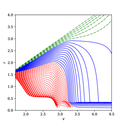
Figure 1: Radius function for constant-$u$ slices in a configuration with $M_{0}=1.0$, $Q=0.9$, $\Lambda=0.06$, $\mu=0$, $A=0.4$, $v_{c}=3.0$ and $w=0.25$. Dashed-dotted green lines reach infinity, full blue lines hit the CH and red dashed lines hit the singularity at $r=0$.

We have evolved the relevant system of equations using the DoNuTS code, described briefly in the Supplemental Material. It is based on the formulation presented in Refs. Burko and Ori (1997); Hansen et al. (2005); Avelino et al. (2011), but the integration technique makes it spectrally accurate in the $v$-direction and, correspondingly, runs with trivial memory requirements and orders of magnitude faster than previously reported codes.

V Results

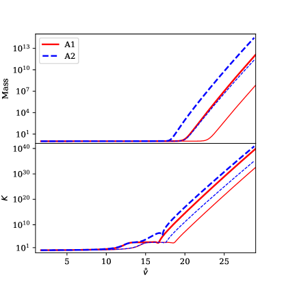
Figure 2: Mass function (10) and Kretschmann scalar as functions of $\overset{\circ}{v}$ for configurations A1 (red solid line) and A2 (blue dashed line). Thin lines are evaluated at $u=u_{\rm EH}+1$ and thick lines are evaluated at $u=u_{\rm EH}+2$. These results are consistent with the existence of mass inflation leading to a weak singularity.

It is important to start by noticing that, as widely expected Costa et al. (2018); Dafermos (2005), our numerics show that all solutions contain a non-empty CH in their BH interior. This can be attested by monitoring the radius function – shown in Fig. 1 – along null lines $u=u_{1}$, for $u_{1}>u_{\rm EH}$, where $u=u_{\rm EH}$ is the event horizon. In fact, for $u_{1}$ larger but close to $u_{\rm EH}$, the radius converges, in $v$, to a non-vanishing constant. It is also interesting to note that, for some initial configurations and large enough $u_{1}$, the radius does converge to zero, signaling (in that region) a singularity beyond which the metric cannot be extended Sbierski (2018).

As is well known the behavior of the scalar field along the event horizon is of great significance for the structure of the BH interior region. The first noteworthy feature of our results (see Supplemental Material for details) is that, as expected, the field decays exponentially (in $\mathring{v}$). More surprisingly, we also clearly observe an oscillatory profile; this might seem odd at first, since it is in contrast with what happens for $\Lambda=0$ and with the expectation created by the study of sufficiently sub-extremal BHs with $0<M^{2}\Lambda\ll 1$ Brady et al. (1997). However, it turns out that such behavior should be expected from the linearized analysis of Refs. Cardoso et al. (2018a, b), where it is shown that, for a configuration resembling our configuration B, there are two modes which dominate the response: a non-oscillatory “near extremal” (NE) mode with characteristic frequency $\omega_{\rm NE}\sim-0.081i$, and a “photon sphere” (PS) mode with $\omega_{\rm PS}\sim 0.096-0.095i$ (these numbers are given in the units and time-coordinate of Ref. Cardoso et al. (2018a)). Here we find very good agreement with the PS mode (when translated to our $\mathring{v}$ coordinate) which is oscillatory in nature. Similar agreement can be found for the remaining configurations A and C. We also recall that, according to the results in Cardoso et al. (2018a), in the $M^{2}\Lambda\ll 1$ case, the dominant mode is a non-oscillatory “de Sitter” mode, in agreement with Brady et al. (1997).

Our main results (concerning mass and curvature) are summarized in Figs. 2-4. Fig. 2 shows the evolution of the mass function and the Kretschmann scalar for configurations A: in these cases mass inflation occurs, and, consequently, the curvature invariant $K$ diverges. Note that an observer crossing one such region will be subjected to physical deformations which are not necessarily infinite (see discussion below). Nonetheless, because there is mass inflation, the singularity is strong enough to deserve the classification of terminal boundary, since it corresponds to a locus where the field equations cease to make sense. These conclusions are consistent with the linear results in Cardoso et al. (2018a) and the nonlinear results in Costa et al. (2018).

Figure 3: Mass function (10) and Kretschmann scalar as functions of $\overset{\circ}{v}$ for configurations B1 (red solid line) and B2 (blue dashed line). Thin lines are evaluated at $u=u_{\rm EH}+1$ and thick lines are evaluated at $u=u_{\rm EH}+2$.

The main novel result of this work concerns Fig. 3: there exist configurations for which no mass inflation occurs. For configurations B, in the BH interior, after a small “accretion” stage the mass settles to a constant value. Moreover, as recently predicted Costa et al. (2018); Cardoso et al. (2018a), the CH remains a curvature singularity, since the curvature scalar $K$ diverges. However, the lack of mass inflation makes the singularity so “mild” that, in principle, one should be able to continue the evolution of the space-time metric across it, by solving the Einstein field equations!

A somewhat unexpected feature (of configuration B) is the oscillatory way in which the curvature scalar diverges. In hindsight, such behavior could be expected from the previously discussed oscillatory behavior of the scalar field along the event horizon. Note that in a no mass inflation situation it is the blow up of $\Phi_{,v}/r_{,v}$ that dominates the behavior of $K$. This should be contrasted with what happens when mass inflation occurs: then it is the monotone divergence of the mass that controls the Kretschmann; this last fact provides an explanation for the non-oscillatory behavior observed for configuration A.

Figure 4: Same as Fig. 3, for configurations C1 (red solid) and C2 (blue dashed).

Concerning massive scalars, the results presented in Fig. 4 identify configuration C as another no mass inflation configuration. Once again we find that the corresponding CH is a “weak” curvature singularity. In fact, the presence of scalar mass seems to have no attenuation effect on the growth of $K$, in contrast with what might be expected from linear analysis Cardoso et al. (2018b) and Dias et al. (2018a).

We finish this section with some further remarks concerning the blow up of curvature. In configuration A, our results indicate that the Kretschmann scalar blows up as $t^{-2}$ (possibly modulated by logarithmic terms), where $t$ is the affine parameter defined in (9) with the Cauchy horizon located at $t=0$. This might suggest that the curvature blows up as $t^{-1}$, but, as noted in Poisson and Israel (1989); Ori (1991), there are curvature components that may blow up even faster. In fact, the quantities that determine the blow-up of the Kretschmann scalar are the square of the (Misner-Sharp) mass $M$ and the square of the gradient of $\Phi$, which is dominated by $(\Phi_{,v}/r_{,v})^{2}$. However, all curvature components are controlled by $M$ and $(\Phi_{,v}/r_{,v})^{2}$ (the origin of the last term can be traced to the energy-momentum tensor). From the behavior of the Kretschmann scalar we can then conclude that the components of the curvature blow up at most as $t^{-2}$; we also expect inverse logarithmic powers Ori (1991); Luk (2018); Dafermos and Luk (2017) that are hard to detect numerically. Although divergent, these curvature components should yield (with the help of the logarithmic terms) a finite “tidal deformation” when integrated twice with respect to $t$, in agreement with the picture in Ori (1991).

From the equation (see Ref. Costa et al. (2017))

$$M_{,v}=\frac{1}{2}\left(1-\frac{2M}{r}+\frac{Q^{2}}{r^{2}}-\frac{\Lambda}{3}r^{2}\right)\left(\frac{\Phi_{,v}}{r_{,v}}\right)^{2}r_{,v}$$ (11)

we conclude that no mass inflation is essentially equivalent to the integrability of $(\Phi_{,v}/r_{,v})^{2}$, with respect to $t$. Moreover, when both occur we immediately see that the curvature can only give rise to finite “tidal deformations”. This reasoning is verified by our results concerning configuration B, for which the mass is bounded, $\Phi_{,v}/r_{,v}$ grows slower than $t^{-1/2}$ and the Kretschmann scalar and the curvature components blow up at most as $t^{-1}$.

VI Discussion

The main motivation for this study was to understand whether nonlinear effects could trigger mass inflation, even when the linearized analysis suggests otherwise Cardoso et al. (2018a). We found that nonlinear effects are not strong enough to change the picture: in fact, the nonlinear results are in full agreement with the linearized predictions. The linearized analysis of Ref. Cardoso et al. (2018a) suggests that no mass inflation should occur for BH charge above a threshold $Q_{*}\simeq 0.95$. Within a nonlinear evolution, the precise linearized results are difficult to reproduce (for instance, the final spacetime parameters depend on the initial parameters and on the size of the initial data). However, for small scalar amplitudes, our results are indeed consistent with the previous threshold.

The (numerical) no mass inflation solutions presented here are the first solutions of this kind arising from the full nonlinear evolution of exterior data. They contain a Cauchy horizon in their BH interior region that can be seen as (“weakly”) singular, due to the divergence of curvature invariants. However, these divergent tidal forces are not necessarily strong enough to lead to a divergent tidal deformation and the consequent unequivocal destruction of all macroscopic objects Ori (1991). Even more problematic, the lack of mass inflation indicates that these Cauchy horizons should maintain enough regularity as to allow the field equations to determine (classically), in a highly non-unique way, the evolution of the metric to their future. This corresponds to a potential severe violation of SCC.

Our results concern spherically symmetric spacetimes. The picture is unlikely to change even with asymmetric initial conditions Cardoso et al. (2018a). Thus, from the conceptual point of view Cardoso et al. (2018b), our results show that SCC is not enforced by the field equations. In the meantime, interesting suggestions to remedy SCC, in the presence of a positive cosmological constant, have been put forward: these include enlarging the allowed set of initial data by weakening their regularity Dafermos and Shlapentokh-Rothman (2018), or restricting the scope of SCC to the uncharged BH setting Dias et al. (2018c). It thus seems plausible that the astrophysical interpretation of SCC remains valid, once other fields and realistic BH charges are considered.

Appendix A Numerical procedure

A.1 Algorithm

Our equations of motion have the form

$$r_{,uv}+\frac{r_{,u}r_{,v}}{r}+\frac{e^{2\sigma}}{2r}\left[1-\frac{Q^{2}}{r^{2}}-\left(\Lambda+\mu^{2}\Phi^{2}\right)r^{2}\right]=0\,,$$ (12)

$$\sigma_{,uv}-\frac{r_{,u}r_{,v}}{r^{2}}-\frac{e^{2\sigma}}{2r^{2}}\left(1-2\frac{Q^{2}}{r^{2}}\right)+\Phi_{,u}\Phi_{,v}=0\,,$$ (13)

$$\Phi_{,uv}+\frac{1}{r}\left(\Phi_{,u}r_{,v}+\Phi_{,v}r_{,u}\right)+\frac{e^{2\sigma}}{2}\mu^{2}\Phi=0\,,$$ (14)

and are subjected to the following constraints

$$r_{,uu}-2r_{,u}\sigma_{,u}+r\,(\Phi_{,u})^{2}=0\,,$$ (15)

$$r_{,vv}-2r_{,v}\sigma_{,v}+r\,(\Phi_{,v})^{2}=0\,.$$ (16)

These equations must be satisfied by the initial data. Then, by virtue of the Bianchi identities, they will be satisfied in the whole computational domain provided that the dynamical equations are accurately satisfied.

To integrate these equations, we start by transforming them into a system of ODEs. Our procedure is as follows. Let $h(u,v)$ be any evolved quantity $r(u,v)$, $\sigma(u,v)$ and $\Phi(u,v)$. Defining $f(v)=\partial_{u}h(u,v)$, all dynamical equations, for fixed $u$, have the form

$$f^{\prime}(v)+f(v)p(v)=g(v)\,,$$ (17)

where ^′ denotes the derivative with respect to $v$. These equations can be solved by introducing the integrating factor

$$\lambda(v)=\exp\left(\int_{v_{i}}^{v}p(v^{\prime})\,dv^{\prime}\right),\qquad\lambda^{\prime}(v)=p(v)\lambda(v)\,.$$

Multiplying Eq. (17) by $\lambda(v)$, we get

$$f^{\prime}(v)\lambda(v)+f(v)\lambda^{\prime}(v)=\left[f(v)\lambda(v)\right]^{\prime}=g(v)\lambda(v)$$

$$\Leftrightarrow f(v)\equiv\partial_{u}h(v)=\frac{1}{\lambda(v)}\left[f(v_{i})+\int_{v_{i}}^{v}g(v^{\prime})\lambda(v^{\prime})\,dv^{\prime}\right]\,,$$

which are ODEs in $u$ for all values of $v$. Given initial conditions in the two null segments $u=u_{i}$, $h(u_{i},v)$ $\forall v$ and $v=v_{i}$, $f(v_{i})\equiv\partial_{u}h(u,v_{i})$ $\forall u$, we can integrate the equations in a rectangular region $u_{i}<u<u_{f}$ and $v_{i}<v<v_{f}$.

For our three functions in Eqs. (12), (13) and (14), $p(v)$ and $g(v)$ are the following:

$$p_{r}(v) =\frac{r_{,v}}{r}\,,$$

$$g_{r}(v) =-\frac{e^{2\sigma}}{2r}\left[1-\frac{Q^{2}}{r^{2}}-\left(\Lambda+\mu^{2}\Phi^{2}\right)r^{2}\right]\,,$$

$$p_{\Phi}(v) =\frac{r_{,v}}{r}\,,$$

$$g_{\Phi}(v) =-\frac{r_{,u}\Phi_{,v}}{r}-\frac{e^{2\sigma}}{2}\mu^{2}\Phi\,,$$

$$p_{\sigma}(v) =0\,,$$

$$g_{\sigma}(v) =\frac{r_{,u}r_{,v}}{r^{2}}+\frac{e^{2\sigma}}{2r^{2}}\left(1-2\frac{Q^{2}}{r^{2}}\right)-\Phi_{,u}\Phi_{,v}\,.$$

We integrate these equations using the Double Null Through Spectral methods (DoNuTS) code written in Julia Bezanson et al. (2017). To integrate the system within DoNuTS, all functions are expanded in a Chebyshev basis in the $v$ direction (where all $v$ derivatives and integrations can be readily performed), and the remaining ODEs in the $u$ direction are integrated using an adaptive step integrator through the DifferentialEquations.jl Julia package Rackauckas and Nie (2017).

A.2 Adaptive gauge

When using the initial gauge, $r_{,u}$ becomes extremely large around the apparent horizon for large $v$. Therefore, in order to explore the near-horizon region at late times, it is convenient to use an adaptive gauge in $u$ during the numerical evolution.

Since the change $u\to\tilde{u}(u)$ together with $\sigma\to\sigma-\frac{1}{2}\log\left(\frac{d\tilde{u}}{du}\right)$ leaves the equations invariant, we can change the gauge in $u$ along the integration by choosing appropriately the initial condition $\sigma_{,u}(u,v_{i})$ at each value of $u$.

To explore the near-horizon geometry, we can choose an Eddington-like gauge for $u$, i.e., a gauge that brings the event horizon to $u\to\infty$. A good way to do so, as described in Eilon and Ori (2016), is to set $\sigma(u,v_{f})=\log\left(2r_{,v}(u,v_{f})\right)+C$, where $C$ can be any constant. In the DoNuTS code, this is achieved by picking the initial condition for $\sigma_{,u}(u,v_{i})$

$$\sigma_{,u}(u,v_{i})=-\left[\sigma(u,v_{f})-\log\left(2r_{,v}(u,v_{f})\right)+\frac{3}{2}\log 2\right]\,.$$ (18)

The term $\frac{3}{2}\log 2$ is chosen so that $\sigma_{,u}(u_{i},v_{i})$ is small when $\sigma(u_{i},v_{f})\approx-\frac{1}{2}\log 2$. With this condition, $\sigma(u,v_{f})$ is damped towards the desired value $\log\left(2r_{,v}(u,v_{f})\right)-\frac{3}{2}\log 2$ along the evolution in $u$. Additionally, in order to satisfy the constraint equation (15), we must introduce an additional ODE for the initial condition $r_{,u}(u,v_{i})$ at $v=v_{i}$,

$$r_{,uu}(u,v_{i})=2r_{,u}(u,v_{i})\sigma_{,u}(u,v_{i})$$ (19)

with $r_{,u}(u_{i},v_{i})=r_{u0}$ obtained using the expression for the Misner-Sharp mass in the main text. By solving this ODE along with all the others, we get the initial conditions at $v=v_{i}$ at each value of $u$ along the integration.

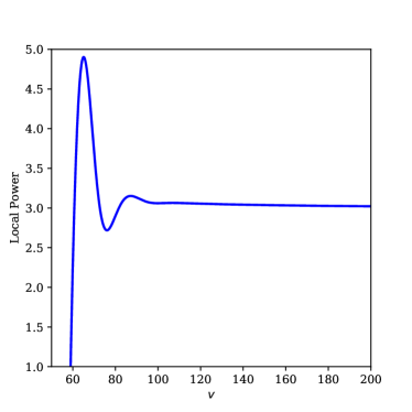
Figure 5: Massless scalar field along the event horizon with corresponding “local power” for a configuration with $M_{0}=1.0$, $Q=0.95$, $\Lambda=0$, $\mu=0$, $A=0.01$, $v_{c}=6.0$ and $w=0.25$. The power-law decay $\Phi\sim v^{-3}$ matches to a very good precision the one expected from linearized analysis Price (1972), and reproduces well previous nonlinear results Burko and Ori (1997).

A.3 Code tests

As a test of our numerical implementation we have reproduced the late-time decay of an asymptotically flat configuration with a massless scalar field. For this, it was crucial to employ the gauge conditions (18), (19). We also compute the “local power” of the scalar field decay, defined as $-v\Phi_{,v}/\Phi$. These are shown in Fig. 5 and are consistent with expected results.

To further test the code, we have analyzed its convergence properties. We thus evaluate the quantity

$$\delta_{n,m}(F)\equiv\max|1-F_{n}/F_{m}|$$ (20)

for a given function $F_{N}$ obtained with resolution $N$ at a fixed $u$ coordinate, and where the maximum is evaluated for all values of $v$. Here, the index $m$ refers to a reference solution obtained using a large number $m$ of grid points while $n$ denotes test solutions using a coarser resolution, $n<m$.

Figure 6: $\delta_{N,64}(K)$ at $u=18.2$ for configuration B1. 20 domains were employed in the $v$ direction, where each domain has $N$ points. The plot clearly shows exponential convergence until $N\approx 40$.

In Fig. 6 we show the convergence properties of the Kretschmann scalar for configurations B1. The plots show exponential convergence up to $N\approx 40$.

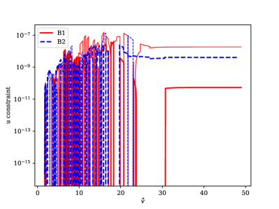
Figure 7: Constraint violations during our evolutions of configurations B.

Finally, since we use a free-evolution scheme, we have checked that the constraint equations (15) and (16) remain satisfied throughout our evolution. We show typical plots for the corresponding constraint violation in Fig. 7.

Appendix B The Kretschmann scalar

To avoid round-off errors we use the expression for the Kretschmann scalar in Costa et al. (2017) (adapted to include a scalar field mass), instead of computing it directly in terms of the metric:

$$K\; \equiv \;R_{\alpha\beta\gamma\delta}R^{\alpha\beta\gamma\delta}=\frac{16}{r^{6}}\left[\left(M-\frac{3Q^{2}}{2r}+\frac{\Lambda}{6}r^{3}\right)+\frac{r}{2}\left(1-\frac{2M}{r}+\frac{Q^{2}}{r^{2}}-\frac{\Lambda}{3}r^{2}\right)\left(\frac{r\Phi_{,u}}{r_{,u}}\right)\left(\frac{r\Phi_{,v}}{r_{,v}}\right)\right]^{2}$$

$$+ \frac{16}{r^{6}}\left(M-\frac{Q^{2}}{2r}+\frac{\Lambda}{6}r^{3}\right)^{2}+\frac{16}{r^{6}}\left(M-\frac{Q^{2}}{r}-\frac{r^{3}}{3}\left(\Lambda+\mu^{2}\Phi^{2}\right)\right)^{2}+\frac{4}{r^{4}}\left(1-\frac{2M}{r}+\frac{Q^{2}}{r^{2}}-\frac{\Lambda}{3}r^{2}\right)^{2}\left(\frac{r\Phi_{,u}}{r_{,u}}\right)^{2}\left(\frac{r\Phi_{,v}}{r_{,v}}\right)^{2}\,,$$

where $M$ is the Misner-Sharp mass.

Appendix C The scalar field along the EH

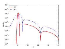
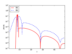
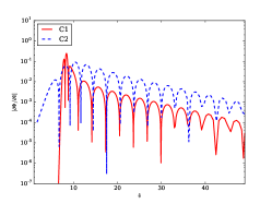
Figure 8: Scalar field derivative $\partial\Phi/\partial\overset{\circ}{v}$ as a function of $\overset{\circ}{v}$ for configurations A (left plot), B (middle plot), C (right plot) with initial profiles 1 (red solid lines) and 2 (blue dashed lines). $\partial\Phi/\partial\overset{\circ}{v}$ evaluated at $u=u_{\rm EH}$.

The scalar field along the event horizon is shown in Fig. 8 (contrast with the asymptotically flat example of Fig. 5). The late-time behavior is described by ringing exponential falloff of the signal, well described by the lowest quasinormal modes of the spacetime Cardoso et al. (2018a).

References

- Costa et al. (2018) J. L. Costa, P. M. Girão, J. Natário, and J. D. Silva, Commun. Math. Phys. 361, 289 (2018), arXiv:1707.08975 [gr-qc] .
- Costa and Franzen (2017) J. L. Costa and A. T. Franzen, Annales Henri Poincare 18, 3371 (2017), arXiv:1607.01018 [gr-qc] .
- Hintz and Vasy (2017) P. Hintz and A. Vasy, J. Math. Phys. 58, 081509 (2017), arXiv:1512.08004 [math.AP] .
- Cardoso et al. (2018a) V. Cardoso, J. L. Costa, K. Destounis, P. Hintz, and A. Jansen, Phys. Rev. Lett. 120, 031103 (2018a), arXiv:1711.10502 [gr-qc] .
- Cardoso et al. (2018b) V. Cardoso, J. L. Costa, K. Destounis, P. Hintz, and A. Jansen, (2018b), arXiv:1808.03631 [gr-qc] .
- Dias et al. (2018a) O. J. C. Dias, H. S. Reall, and J. E. Santos, (2018a), arXiv:1808.02895 [gr-qc] .
- Mo et al. (2018) Y. Mo, Y. Tian, B. Wang, H. Zhang, and Z. Zhong, (2018), arXiv:1808.03635 [gr-qc] .
- Dias et al. (2018b) O. J. C. Dias, H. S. Reall, and J. E. Santos, (2018b), arXiv:1808.04832 [gr-qc] .
- Mellor and Moss (1990) F. Mellor and I. Moss, Phys. Rev. D41, 403 (1990).
- Brady et al. (1998) P. R. Brady, I. G. Moss, and R. C. Myers, Phys. Rev. Lett. 80, 3432 (1998), arXiv:gr-qc/9801032 [gr-qc] .
- Dafermos (2005) M. Dafermos, Commun. Pure Appl. Math. 58, 0445 (2005), arXiv:gr-qc/0307013 [gr-qc] .
- Luk (2018) J. Luk, J. Am. Math. Soc. 31, 1 (2018), arXiv:1311.4970 [gr-qc] .
- Dafermos and Luk (2017) M. Dafermos and J. Luk, (2017), arXiv:1710.01722 [gr-qc] .
- Luk and Oh (2017a) J. Luk and S.-J. Oh, (2017a), arXiv:1702.05715 [gr-qc] .
- Luk and Oh (2017b) J. Luk and S.-J. Oh, (2017b), arXiv:1702.05716 [gr-qc] .
- Van de Moortel (2017) M. Van de Moortel, (2017), 10.1007/s00220-017-3079-3, arXiv:1704.05790 [gr-qc] .
- Dafermos (2014) M. Dafermos, Commun. Math. Phys. 332, 729 (2014), arXiv:1201.1797 [gr-qc] .
- Klainerman et al. (2015) S. Klainerman, I. Rodnianski, and J. Szeftel, Invent. Math. 202, 91 (2015), arXiv:1204.1767 [math.AP] .
- Ori (1991) A. Ori, Phys. Rev. Lett. 67, 789 (1991).
- Burko and Ori (1997) L. M. Burko and A. Ori, Phys. Rev. D56, 7820 (1997), arXiv:gr-qc/9703067 [gr-qc] .
- Hansen et al. (2005) J. Hansen, A. Khokhlov, and I. Novikov, Phys. Rev. D71, 064013 (2005), arXiv:gr-qc/0501015 [gr-qc] .
- Avelino et al. (2011) P. P. Avelino, A. J. S. Hamilton, C. A. R. Herdeiro, and M. Zilhao, Phys. Rev. D84, 024019 (2011), arXiv:1105.4434 [gr-qc] .
- Sbierski (2018) J. Sbierski, J. Diff. Geom. 108, 319 (2018), arXiv:1507.00601 [gr-qc] .
- Brady et al. (1997) P. R. Brady, C. M. Chambers, W. Krivan, and P. Laguna, Phys. Rev. D55, 7538 (1997), arXiv:gr-qc/9611056 [gr-qc] .
- Poisson and Israel (1989) E. Poisson and W. Israel, Phys. Rev. Lett. 63, 1663 (1989).
- Costa et al. (2017) J. L. Costa, P. M. Girão, J. Natário, and J. D. Silva, Ann. PDE 3 (2017), 10.1007/s40818-017-0028-6, arXiv:1406.7261 [gr-qc] .
- Dafermos and Shlapentokh-Rothman (2018) M. Dafermos and Y. Shlapentokh-Rothman, (2018), arXiv:1805.08764 [gr-qc] .
- Dias et al. (2018c) O. J. C. Dias, F. C. Eperon, H. S. Reall, and J. E. Santos, Phys. Rev. D97, 104060 (2018c), arXiv:1801.09694 [gr-qc] .
- Bezanson et al. (2017) J. Bezanson, A. Edelman, S. Karpinski, and V. B. Shah, SIAM review 59, 65 (2017).
- Rackauckas and Nie (2017) C. Rackauckas and Q. Nie, Journal of Open Research Software 5 (2017), 10.5334/jors.151.
- Eilon and Ori (2016) E. Eilon and A. Ori, Phys. Rev. D93, 024016 (2016), arXiv:1510.05273 [gr-qc] .
- Price (1972) R. H. Price, Phys. Rev. D5, 2419 (1972).