Extended Optical/NIR Observations of Type Iax Supernova 2014dt: Possible Signatures of a Bound Remnant

Abstract

We present optical and near-infrared observations of the nearby Type Iax supernova (SN) 2014dt from $14$ to $410$ days after the maximum light. The velocities of the iron absorption lines in the early phase indicated that SN 2014dt showed slower expansion than the well-observed Type Iax SNe 2002cx, 2005hk and 2012Z. In the late phase, the evolution of the light curve and that of the spectra were considerably slower. The spectral energy distribution kept roughly the same shape after $\sim 100$ days, and the bolometric light curve flattened during the same period. These observations suggest the existence of an optically thick component that almost fully trapped the $\gamma$-ray energy from ⁵⁶Co decay. These findings are consistent with the predictions of the weak deflagration model, leaving a bound white dwarf remnant after the explosion.

1 Introduction

For normal Type Ia supernovae (SNe Ia), there is a well-established correlation between the peak luminosity and the decline rate of the light curve (LC; e.g., Phillips 1993), which has been used to measure distances to remote galaxies. However, some SNe Ia deviate from this correlation, and their peak luminosities are significantly fainter ($\geq$ 1 mag) than those of normal SNe Ia with similar decline rates. These outliers have been called SN 2002cx-like SNe (Li et al. 2003) or SNe Iax (Foley et al. 2013). SNe Iax commonly show lower luminosities, lower expansion velocities and hotter photospheres around their maximum light than normal SNe Ia (Foley et al. 2013 and references therein), as well as scatter in maximum magnitudes and decline rates. For example, the maximum magnitude of the faintest SN Iax 2008ha is only $-13.74\pm 0.15$ mag in the $B$-band (Foley et al. 2009), which is $\sim$ 4 mag fainter than that of the prototypical SN Iax SN 2002cx. The line velocities of SNe Iax around the maximum light are $2000$–$8000$ km s^-1, whereas those of normal SNe Ia are $\gtrsim 10000$ km s^-1. The estimated ⁵⁶Ni mass and explosion energy of SNe Iax are only $0.003$–$0.3$ M_⊙ and $10^{49}$–$10^{51}$ erg, respectively (e.g., Foley et al. 2009, Foley et al. 2013, Stritzinger et al. 2015).

From the compilation of early phase observations of SNe Iax, weak correlations between the maximum magnitude and the decline rate, line velocity and rising time have been suggested (e.g., Narayan et al. 2011; Foley et al. 2013; Magee et al. 2016). However, rapidly increasing observational data suggest that this is probably an oversimplification and that SNe Iax show large diversity as well. For example, SN Iax 2014ck showed spectra similar to SN 2008ha, whereas the LCs were similar to SNe 2002cx and 2005hk (Tomasella et al. 2016). PS1-12bwh showed a spectral evolution similar to that of SN 2005hk in the post-maximum phase, whereas the pre-maximum evolution showed significant difference (Magee et al. 2017). SN 2012Z showed close similarity to SN 2005hk in its early phase spectra. In the late phase, although the emission lines of SN 2012Z were significantly broader than those of SN 2005hk, the overall spectral features of SN 2012Z were similar to those of SN 2005hk. Regardless of the similarity seen in the spectra, the decline rates of the LCs in the late phase show the diversity (Stritzinger et al. 2015, Yamanaka et al. 2015).

These peculiarities of SNe Iax are difficult to explain within the framework of canonical SNe Ia. Many researchers have discussed plausible models that can reproduce the observed properties. One of the models is the weak deflagration of a Chandrasekhar-mass carbon-oxygen white dwarf (e.g., Fink et al. 2014), in which a considerable part of the white dwarf could not gain sufficient kinetic energy to exceed the binding energy, and a bound white dwarf remnant of $\sim$ 1 M_⊙ may be left after the explosion. However, Valenti et al. (2009) suggested that a fraction of SNe Iax could be core-collapse (CC) SNe based on of some characteristics in the optical spectra. Moriya et al. (2010) suggested a ‘fallback CC SN model’ for SNe Iax, where a considerable fraction of the ejecta would fall onto the central remnant, probably a black hole, in a CC SN explosion of a massive star ($\gtrsim$ 25 M_⊙).

To date, the number of SNe Iax for which the evolution of the late phases has been well-observed remains small. Late phase observations are expected to carry important information on the progenitor and explosion through a direct view to the inner part of the ejecta (e.g., Maeda et al. 2010). The spectra of some SNe Iax in the late phase show the permitted lines with the P-Cygni profile, unlike those of SNe Ia. From the analysis of the late phase spectra, Foley et al. (2016) suggested that the ejecta of SNe Iax have two distinct components, one of which creates the photosphere even in the late phase. Thus, the data for SNe Iax in the late phases can provide meaningful constraints on an explosion model. In addition, the low expansion velocity in SNe Iax makes it easier to identify different subclasses than in SNe Ia due to the smaller contamination by line blending (e.g., Stritzinger et al. 2014; but see Szalai et al. 2015 for practical difficulties in this kind of analysis).

The recent apparent identification of possible progenitor systems for two SNe Iax could be important for exploring the explosion model and links to normal SNe Ia. For SN 2012Z, a blue hot star (possibly a companion helium star) has been detected in pre-explosion images (McCully et al. 2014). For SN 2008ha, a luminous redder source has appeared in the post-explosion images, which could be a bound remnant or a survived companion star (Foley et al. 2014). For other SN Iax (SN 2008ge; Foley et al. 2010 and SN 2014ck; Tomasella et al. 2016), only the upper limits for the brightness of the progenitors have been derived, excluding a massive progenitor scenario.

SN 2014dt was discovered by K. Itagaki in a nearby galaxy M61 on 2014 October 29.8 (UT) at 13.6 mag (Nakano et al. 2014). The spectrum obtained on October 31, 2014, by the Asiago Supernova classification program is consistent with a SN Iax at $\sim$ 1 week after the maximum light (Ochner et al. 2014). SN 2014dt is one of the nearest SN Iax ever discovered (see below). Foley et al. (2015) gave an upper limit for the luminosity of the progenitor system using pre-explosion images taken with the Hubble Space Telescope (HST), which is consistent with a system with a low-mass evolved or main-sequence companion. However, the upper limit could not reject the system with a sub-class of Wolf-Rayet star. The distance of M61 obtained by several works are summarized in the NASA/IPAC Extragalactic Database (NED). The Tully-Fisher relation (Schoeniger & Sofue 1997) shows a large scatter ($\mu=30.02\pm 0.92$ mag using the CO Tully-Fisher relation, and $\mu=30.21\pm 0.70$ mag using the Hi Tully-Fisher relation), thus we decided not to adopt these values. Bose & Kumar et al. (2014) reported the distance obtained by applying the expanding photosphere method (EPM) to SN 2008in (Bose & Kumar et al. 2014). They gave two possible values for the distance with two different atmosphere models, $\mu=30.45\pm 0.10$ mag and $\mu=30.81\pm 0.20$ mag. In this paper, we adopt the EPM distance of M61, $\mu=30.81\pm 0.20$ mag, which was calibrated with the atmosphere model updated by Dessart & Hillier (2005). Some parameters (e.g., the luminosity, the ⁵⁶Ni mass) are affected by the difference of the adopted distance. In this paper we adopt the EPM distance, while the parameter values derived with the Tully-Fisher distances will be mentioned as well to show associated uncertainty. For the total extinction towards SN 2014dt, we simply adopted $E(B-V)_{\rm total}=0.02$ mag, following Foley et al. (2015).

In this paper, we report our extended optical and near-infrared (NIR) observations of SN 2014dt. We describe the observation and data reduction in §2. In §3, we present the results of our observations. In §4, we investigate the characteristic features of SN 2014dt and discuss the implications for the progenitor and explosion mechanism. In the analyses, we emphasize the characteristic behaviors found in the late phase. The slow evolution seen in the LCs and spectral energy distribution (SED) suggests the existence of high-density material buried deep in the ejecta. A similar suggestion was made by Foley et al. (2016), based on late phase spectra, but our conclusions were reached by independent observational materials. A summary of this work is provided in §5.

2 Observations and Data Reduction

We performed optical $BVRI$-band photometry of SN 2014dt using Hiroshima One-shot Wide-field Polarimeter (HOWPol; Kawabata et al. 2008) installed at the 1.5 m Kanata telescope at Higashi-Hiroshima Observatory and with an Andor DW936N-BV CCD camera installed at the 51 cm telescope at Osaka Kyoiku University (OKU). We reduced the data in a standard manner for CCD photometry. For the images obtained by HOWPol, we performed subtraction of the host galaxy template image before aperture photometry to minimize contamination by the host galaxy background (Figure 2). The template images for the $BVRI$-bands were obtained with the same telescope and instrument on 2018 February 23 (i.e., $>1200$ days after the discovery; Figure 2). We removed the cosmic rays using L. A. Cosmic pipeline (van Dokkum 2001, van Dokkum et al. 2012). After that, we remapped our data to WCS using the SExtractor (Bertin & Arnouts 1996), and transformed the template images into our images using $wcsremap$. The host galaxy subtraction was then performed using $hotpants$ . For the subsequent aperture photometry, we used the DAOPHOT package in IRAF. We estimated the error for the photometry from the error associated with photometry, the variation in the magnitude obtained from each comparison stars and the difference images. The error for the photometry included that caused by the host galaxy subtraction. The estimated error due to the host galaxy subtraction is dominant.

For the images obtained by Andor CCD camera on the 51cm telescope, we skipped the template subtraction because the images were significantly affected by fringe patterns and the template subtraction made the photometric results worse. We, however, note that the host galaxy contamination is negligible for those images, as those were obtained in the early phases when the SN itself was much brighter than the host background (as was confirmed by the subtracted images for the HOWPol data). We adopted Point-Spread-Function (PSF) fitting photometry for these data.

For the magnitude calibration, we adopted relative photometry using comparison stars taken in the same frame (Figure 1). The magnitudes of the comparison stars were calibrated with the photometric standard stars in the Landolt field (SA104; Landolt 1992), observed on photometric nights using HOWPol. We show the magnitudes of the comparison stars in Table 1. The magnitudes are consistent with those reported by Roy et al. (2011). We note that the $B$-band magnitudes of the comparison stars, as well as those given by Roy et al. (2011), are $\sim$0.3 mag fainer those shows given by Singh et al. (2018), perhaps due to a systematic difference between the systems. For photometric correction, we performed first-order color term correction. We skipped S-correction, which is negligible for the purposes of this study (Stritzinger et al. 2002). We list the journal of the optical photometry in Table 2.

We performed NIR $JHK_{s}$-band photometry with Hiroshima Optical and Near-InfraRed camera (HONIR; Akitaya et al. 2014) installed at the 1.5 m Kanata telescope. In the observations, we adopted five-position dithering method. We adopted the host galaxy subtraction and the aperture photometry method in the same way as used for reduction of the optical data, and calibrated the magnitude of the SN using the comparison stars in the 2MASS catalog (Skrutskie et al. 2006). We obtained the galaxy template images with the same telescope and instrument on 2017 April 23 (i.e., at $>900$ days after the discovery; Figure 2). For the photometric error, we included the error caused by the host galaxy in the same way as for the HOWPol data. The journal of NIR photometry is shown in Table 3.

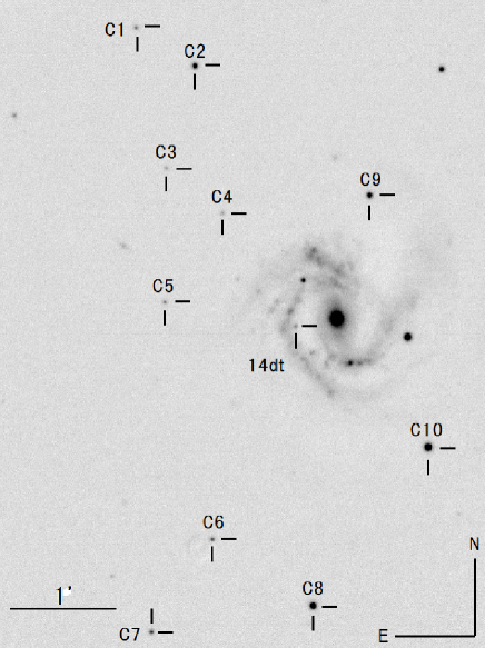
Figure 1: The $R$-band image of SN 2014dt and comparison stars taken with the Kanata telescope/HOWPol on MJD 57171.51 (2015 March 29).

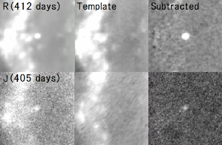
Figure 2: Comparison of the observed (left panels), the template (center), and the subtracted (right) images around SN 2014dt. Upper and lower panels are images in the $R$-band at 412 days and in the $J$-band at 405 days, respectively. The field of view is $30^{\prime\prime}\times 30^{\prime\prime}$. The template image in the $R$-band is synthesized from SDSS images, and that in the $J$-band was obtained with HONIR (see text).

lccccccc Magnitudes of comparison stars of SN 2014dt ID $B$ (mag) $V$ (mag) $R$ (mag) $I$ (mag) $J$ (mag) $H$ (mag) $K_{s}$ (mag)
The magnitudes in the NIR bands are from the 2MASS catalog (Skrutskie et al. 2006). C1 17.536 $\pm$ 0.026 16.842 $\pm$ 0.012 16.338 $\pm$ 0.024 15.992 $\pm$ 0.012 $-$ $-$ $-$
C2 16.340 $\pm$ 0.023 15.505 $\pm$ 0.010 14.970 $\pm$ 0.034 14.533 $\pm$ 0.016 $-$ $-$ $-$
C3 18.451 $\pm$ 0.033 17.682 $\pm$ 0.015 17.170 $\pm$ 0.025 16.812 $\pm$ 0.014 $-$ $-$ $-$
C4 19.585 $\pm$ 0.066 18.053 $\pm$ 0.019 16.971 $\pm$ 0.025 16.061 $\pm$ 0.012 15.261 $\pm$ 0.055 14.571 $\pm$ 0.070 14.377 $\pm$ 0.099
C5 18.785 $\pm$ 0.039 17.552 $\pm$ 0.014 16.575 $\pm$ 0.024 15.872 $\pm$ 0.012 15.135 $\pm$ 0.059 14.598 $\pm$ 0.051 14.343 $\pm$ 0.087
C6 18.280 $\pm$ 0.032 16.956 $\pm$ 0.012 15.977 $\pm$ 0.024 15.252 $\pm$ 0.011 14.619 $\pm$ 0.042 13.956 $\pm$ 0.038 13.831 $\pm$ 0.061
C7 18.256 $\pm$ 0.032 16.895 $\pm$ 0.012 15.878 $\pm$ 0.024 15.144 $\pm$ 0.011 $-$ $-$ $-$
C8 15.542 $\pm$ 0.023 14.731 $\pm$ 0.010 14.164 $\pm$ 0.024 13.748 $\pm$ 0.011 13.525 $\pm$ 0.026 13.115 $\pm$ 0.028 13.053 $\pm$ 0.035
C9 16.844 $\pm$ 0.024 15.609 $\pm$ 0.010 14.719 $\pm$ 0.024 14.048 $\pm$ 0.011 13.326 $\pm$ 0.023 12.724 $\pm$ 0.026 12.602 $\pm$ 0.033
C10 $-$ $-$ $-$ $-$ 12.734 $\pm$ 0.026 12.388 $\pm$ 0.030 12.352 $\pm$ 0.031

We obtained optical spectra of SN 2014dt using HOWPol at 13 epochs. The wavelength coverage was $4500$–$9200$ Å and the wavelength resolution was $R=\lambda/\Delta\lambda\simeq 400$ at 6000 Å. For wavelength calibration, we used sky emission lines. To remove cosmic ray events, we used the L. A. Cosmic pipeline. The flux of SN 2014dt was calibrated using data of spectrophotometric standard stars taken on the same night. The journal of spectroscopy is listed in Table 4.

In addition, we obtained optical photometric and spectroscopic data in the late phases with the Faint Object Camera and Spectrograph (FOCAS; Kashikawa et al. 2002) installed at the 8.2 m Subaru telescope, NAOJ. The wavelength resolution was $R=\lambda/\Delta\lambda\simeq 650$ at 6000 Å. The data reduction was performed in the same way as that with HOWPol, except for the host galaxy subtraction for the imaging photometry and the wavelength calibration for the spectroscopy. The template images for the $V$ and $R$-bands were created from the SDSS $u^{\prime}g^{\prime}r^{\prime}i^{\prime}z^{\prime}$ images using the relations for the flux transformation (Smith et al. 2002). For the wavelength calibration, we used arc lamp (Th-Ar) data and skylines. The observation log with Subaru/FOCAS is shown in Tables 2 and 4.

lccccccc Log of optical photometry of SN 2014dt Date MJD Phase $B$ (mag) $V$ (mag) $R$ (mag) $I$ (mag) Site
The uncertainty of phase is inevitably larger, $\pm 4$ days. See §3.3. See §2. 2014-11-03 56964.85 14.4 $-$ $-$ 13.43 $\pm$ 0.03 13.31 $\pm$ 0.02 OKU
2014-11-04 56965.84 15.4 $-$ $-$ 13.51 $\pm$ 0.04 13.37 $\pm$ 0.01 OKU
2014-11-05 56966.83 16.4 $-$ $-$ 13.654 $\pm$ 0.051 13.313 $\pm$ 0.050 Kanata
2014-11-06 56967.86 17.5 $-$ 14.349 $\pm$ 0.054 13.743 $\pm$ 0.055 13.312 $\pm$ 0.051 Kanata
2014-11-10 56971.84 22.4 16.113 $\pm$ 0.050 14.522 $\pm$ 0.050 13.965 $\pm$ 0.051 13.580 $\pm$ 0.051 Kanata
2014-11-10 56971.85 22.4 $-$ 14.65 $\pm$ 0.07 13.97 $\pm$ 0.04 13.63 $\pm$ 0.04 OKU
2014-11-13 56974.84 24.4 $-$ $-$ 14.165 $\pm$ 0.050 13.894 $\pm$ 0.120 Kanata
2014-11-16 56977.83 27.4 $-$ 14.95 $\pm$ 0.03 14.23 $\pm$ 0.05 13.81 $\pm$ 0.03 OKU
2014-11-17 56978.86 28.5 $-$ $-$ 14.34 $\pm$ 0.03 14.03 $\pm$ 0.02 OKU
2014-11-18 56979.85 29.4 16.54 $\pm$ 0.04 14.98 $\pm$ 0.02 14.35 $\pm$ 0.03 14.02 $\pm$ 0.02 OKU
2014-11-18 56979.85 29.4 16.594 $\pm$ 0.054 15.125 $\pm$ 0.051 14.380 $\pm$ 0.050 13.964 $\pm$ 0.050 Kanata
2014-11-19 56980.84 30.4 $-$ 15.02 $\pm$ 0.08 $-$ $-$ OKU
2014-11-20 56981.84 31.4 16.68 $\pm$ 0.06 15.02 $\pm$ 0.03 14.42 $\pm$ 0.03 14.12 $\pm$ 0.02 OKU
2014-11-22 56983.84 33.4 16.846 $\pm$ 0.050 $-$ $-$ $-$ Kanata
2014-11-22 56983.85 33.4 16.68 $\pm$ 0.07 15.11 $\pm$ 0.01 14.54 $\pm$ 0.03 14.11 $\pm$ 0.10 OKU
2014-11-23 56984.83 34.4 16.82 $\pm$ 0.08 15.14 $\pm$ 0.03 14.54 $\pm$ 0.03 14.23 $\pm$ 0.02 OKU
2014-11-27 56988.84 38.4 16.77 $\pm$ 0.06 15.25 $\pm$ 0.03 14.70 $\pm$ 0.03 14.37 $\pm$ 0.02 OKU
2014-11-29 56990.85 40.4 16.73 $\pm$ 0.06 15.33 $\pm$ 0.02 14.78 $\pm$ 0.03 14.48 $\pm$ 0.05 OKU
2014-11-29 56990.87 40.5 16.848 $\pm$ 0.050 $-$ $-$ $-$ Kanata
2014-12-05 56996.86 46.5 16.80 $\pm$ 0.03 15.44 $\pm$ 0.02 14.94 $\pm$ 0.05 $-$ OKU
2014-12-06 56997.80 47.4 17.10 $\pm$ 0.05 15.48 $\pm$ 0.03 15.03 $\pm$ 0.03 14.72 $\pm$ 0.02 OKU
2014-12-07 56998.86 48.5 16.87 $\pm$ 0.06 15.49 $\pm$ 0.01 15.03 $\pm$ 0.03 14.72 $\pm$ 0.02 OKU
2014-12-07 56998.86 48.5 17.020 $\pm$ 0.054 $-$ $-$ $-$ Kanata
2014-12-08 56999.84 49.4 16.90 $\pm$ 0.04 15.49 $\pm$ 0.03 $-$ $-$ OKU
2014-12-11 57002.80 52.4 17.08 $\pm$ 0.08 15.58 $\pm$ 0.06 15.13 $\pm$ 0.03 14.81 $\pm$ 0.01 OKU
2014-12-13 57004.81 54.4 16.98 $\pm$ 0.04 15.60 $\pm$ 0.02 15.17 $\pm$ 0.03 15.05 $\pm$ 0.31 OKU
2014-12-14 57005.86 55.5 17.09 $\pm$ 0.04 15.63 $\pm$ 0.02 15.19 $\pm$ 0.03 14.89 $\pm$ 0.02 OKU
2014-12-20 57011.86 61.5 17.068 $\pm$ 0.050 15.931 $\pm$ 0.052 15.425 $\pm$ 0.051 14.880 $\pm$ 0.051 Kanata
2014-12-21 57012.80 62.4 17.00 $\pm$ 0.08 15.81 $\pm$ 0.05 15.38 $\pm$ 0.04 15.06 $\pm$ 0.01 OKU
2014-12-22 57013.85 63.4 17.22 $\pm$ 0.21 15.67 $\pm$ 0.22 15.40 $\pm$ 0.03 15.01 $\pm$ 0.10 OKU
2014-12-23 57014.83 64.4 17.01 $\pm$ 0.03 15.79 $\pm$ 0.02 15.41 $\pm$ 0.04 15.10 $\pm$ 0.02 OKU
2014-12-24 57015.87 65.5 17.15 $\pm$ 0.11 15.86 $\pm$ 0.05 15.48 $\pm$ 0.06 $-$ OKU
2014-12-26 57017.78 67.4 16.98 $\pm$ 0.03 15.87 $\pm$ 0.02 15.47 $\pm$ 0.04 15.05 $\pm$ 0.08 OKU
2014-12-26 57017.87 68.4 17.099 $\pm$ 0.050 16.078 $\pm$ 0.051 15.541 $\pm$ 0.051 14.984 $\pm$ 0.050 Kanata
2014-12-27 57018.80 68.4 17.18 $\pm$ 0.03 15.84 $\pm$ 0.03 15.48 $\pm$ 0.03 15.20 $\pm$ 0.01 OKU
2014-12-29 57020.80 70.4 17.18 $\pm$ 0.06 15.93 $\pm$ 0.01 15.56 $\pm$ 0.03 15.26 $\pm$ 0.01 OKU
2014-12-30 57021.83 71.4 17.24 $\pm$ 0.04 15.96 $\pm$ 0.02 15.59 $\pm$ 0.03 15.29 $\pm$ 0.02 OKU
2015-01-02 57024.86 74.4 17.27 $\pm$ 0.15 $-$ $-$ $-$ OKU
2015-01-03 57025.80 75.4 17.11 $\pm$ 0.15 $-$ $-$ $-$ OKU
2015-01-04 57026.83 76.4 17.34 $\pm$ 0.04 16.02 $\pm$ 0.02 15.70 $\pm$ 0.03 $-$ OKU
2015-01-08 57030.86 80.5 17.36 $\pm$ 0.04 $-$ $-$ $-$ OKU
2015-01-10 57032.80 82.4 17.49 $\pm$ 0.07 16.03 $\pm$ 0.12 15.80 $\pm$ 0.03 15.41 $\pm$ 0.02 OKU
2015-01-10 57032.83 82.4 17.778 $\pm$ 0.054 16.334 $\pm$ 0.051 16.002 $\pm$ 0.051 15.348 $\pm$ 0.050 Kanata
2015-01-16 57035.79 85.4 17.25 $\pm$ 0.07 16.14 $\pm$ 0.03 15.86 $\pm$ 0.03 15.47 $\pm$ 0.02 OKU
2015-01-17 57038.76 88.4 17.41 $\pm$ 0.04 $-$ $-$ $-$ OKU
2015-01-20 57039.82 89.4 17.32 $\pm$ 0.04 16.32 $\pm$ 0.06 15.93 $\pm$ 0.04 15.58 $\pm$ 0.02 OKU
2015-01-23 57042.76 92.4 17.42 $\pm$ 0.05 16.25 $\pm$ 0.03 15.96 $\pm$ 0.11 15.34 $\pm$ 0.06 OKU
2015-01-24 57045.82 96.3 17.34 $\pm$ 0.06 16.31 $\pm$ 0.02 16.06 $\pm$ 0.06 $-$ OKU
2015-01-24 57046.67 96.3 17.506 $\pm$ 0.050 16.665 $\pm$ 0.052 $-$ 15.484 $\pm$ 0.051 Kanata
2015-01-24 57046.69 96.3 17.51 $\pm$ 0.05 16.34 $\pm$ 0.02 16.08 $\pm$ 0.04 $-$ OKU
2015-01-28 57050.71 100.3 17.31 $\pm$ 0.16 16.35 $\pm$ 0.04 15.99 $\pm$ 0.09 $-$ OKU
2015-01-31 57053.77 103.4 17.61 $\pm$ 0.03 16.44 $\pm$ 0.02 16.20 $\pm$ 0.05 $-$ OKU
2015-02-01 57054.75 104.3 17.57 $\pm$ 0.04 $-$ $-$ $-$ OKU
2015-02-01 57054.76 104.4 17.560 $\pm$ 0.059 16.699 $\pm$ 0.056 $-$ $-$ Kanata
2015-02-06 57059.72 109.3 $-$ 16.61 $\pm$ 0.04 16.31 $\pm$ 0.03 $-$ OKU
2015-02-10 57063.71 113.3 17.74 $\pm$ 0.04 16.61 $\pm$ 0.02 $-$ $-$ OKU
2015-02-11 57064.75 114.3 $-$ $-$ 16.22 $\pm$ 0.07 $-$ OKU
2015-02-12 57065.75 115.3 17.68 $\pm$ 0.03 16.51 $\pm$ 0.12 16.40 $\pm$ 0.13 $-$ OKU
2015-02-13 57066.69 116.3 17.744 $\pm$ 0.050 16.793 $\pm$ 0.051 $-$ $-$ Kanata
2015-02-13 57066.81 116.4 17.77 $\pm$ 0.09 16.61 $\pm$ 0.03 16.29 $\pm$ 0.07 $-$ OKU
2015-02-14 57067.74 117.3 17.75 $\pm$ 0.03 16.65 $\pm$ 0.02 16.39 $\pm$ 0.04 $-$ OKU
2015-02-19 57072.67 122.3 17.65 $\pm$ 0.13 16.64 $\pm$ 0.06 16.40 $\pm$ 0.03 $-$ OKU
2015-02-20 57073.72 123.3 17.77 $\pm$ 0.05 16.68 $\pm$ 0.03 16.38 $\pm$ 0.05 $-$ OKU
2015-02-23 57076.70 126.3 17.90 $\pm$ 0.03 16.73 $\pm$ 0.03 16.50 $\pm$ 0.05 $-$ OKU
2015-02-24 57077.67 127.3 17.54 $\pm$ 0.05 16.50 $\pm$ 0.03 16.19 $\pm$ 0.05 $-$ OKU
2015-02-26 57079.83 129.4 18.120 $\pm$ 0.050 17.101 $\pm$ 0.054 16.615 $\pm$ 0.053 15.889 $\pm$ 0.053 Kanata
2015-03-01 57082.68 132.3 17.864 $\pm$ 0.050 17.169 $\pm$ 0.059 16.637 $\pm$ 0.058 15.845 $\pm$ 0.052 Kanata
2015-03-01 57082.74 132.3 17.56 $\pm$ 0.27 16.86 $\pm$ 0.15 16.48 $\pm$ 0.08 $-$ OKU
2015-03-02 57083.72 133.3 $-$ 16.83 $\pm$ 0.02 16.47 $\pm$ 0.05 $-$ OKU
2015-03-04 57085.78 135.4 $-$ 16.82 $\pm$ 0.08 $-$ $-$ OKU
2015-03-10 57091.65 141.2 17.76 $\pm$ 0.23 16.87 $\pm$ 0.04 16.61 $\pm$ 0.06 $-$ OKU
2015-03-11 57092.69 142.3 18.03 $\pm$ 0.03 16.98 $\pm$ 0.03 $-$ $-$ OKU
2015-03-12 57093.60 143.2 $-$ 16.97 $\pm$ 0.02 16.69 $\pm$ 0.04 $-$ OKU
2015-03-14 57095.66 145.3 $-$ 16.90 $\pm$ 0.19 $-$ $-$ OKU
2015-03-16 57097.59 147.2 $-$ 16.98 $\pm$ 0.02 16.68 $\pm$ 0.05 16.17 $\pm$ 0.03 OKU
2015-03-17 57098.59 148.2 $-$ 17.05 $\pm$ 0.05 16.67 $\pm$ 0.06 16.30 $\pm$ 0.27 OKU
2015-03-20 57101.62 151.2 $-$ 16.97 $\pm$ 0.04 16.71 $\pm$ 0.03 16.19 $\pm$ 0.04 OKU
2015-03-21 57102.53 152.1 $-$ 17.238 $\pm$ 0.056 16.757 $\pm$ 0.052 15.955 $\pm$ 0.052 Kanata
2015-03-21 57102.62 152.2 $-$ 17.03 $\pm$ 0.07 16.75 $\pm$ 0.07 16.19 $\pm$ 0.11 OKU
2015-03-22 57103.69 153.3 $-$ 17.05 $\pm$ 0.08 16.68 $\pm$ 0.05 16.19 $\pm$ 0.06 OKU
2015-03-23 57104.59 154.2 $-$ 17.00 $\pm$ 0.08 16.63 $\pm$ 0.05 16.14 $\pm$ 0.02 OKU
2015-03-24 57105.58 155.2 $-$ 17.07 $\pm$ 0.11 16.75 $\pm$ 0.05 16.21 $\pm$ 0.04 OKU
2015-03-25 57106.56 156.2 $-$ 17.13 $\pm$ 0.05 16.75 $\pm$ 0.06 16.25 $\pm$ 0.03 OKU
2015-03-26 57107.53 157.1 $-$ 17.12 $\pm$ 0.08 16.82 $\pm$ 0.04 16.33 $\pm$ 0.04 OKU
2015-03-27 57108.55 158.1 $-$ 17.01 $\pm$ 0.13 16.73 $\pm$ 0.07 16.11 $\pm$ 0.14 OKU
2015-03-28 57109.57 159.2 18.28 $\pm$ 0.05 17.11 $\pm$ 0.08 16.81 $\pm$ 0.05 16.34 $\pm$ 0.05 OKU
2015-03-28 57109.60 159.2 $-$ $-$ 16.529 $\pm$ 0.056 $-$ Kanata
2015-03-29 57110.61 160.2 18.297 $\pm$ 0.085 17.215 $\pm$ 0.062 16.787 $\pm$ 0.061 15.993 $\pm$ 0.056 Kanata
2015-03-30 57111.59 161.2 18.25 $\pm$ 0.12 17.07 $\pm$ 0.05 16.79 $\pm$ 0.03 16.30 $\pm$ 0.03 OKU
2015-04-11 57123.53 173.1 $-$ 17.19 $\pm$ 0.09 16.87 $\pm$ 0.20 16.31 $\pm$ 0.11 OKU
2015-04-21 57133.53 183.1 18.780 $\pm$ 0.050 17.509 $\pm$ 0.078 17.127 $\pm$ 0.057 16.250 $\pm$ 0.052 Kanata
2015-05-05 57147.46 197.1 19.000 $\pm$ 0.050 17.629 $\pm$ 0.059 $-$ $-$ Kanata
2015-05-29 57171.51 221.1 19.571 $\pm$ 0.087 18.013 $\pm$ 0.052 17.269 $\pm$ 0.051 16.557 $\pm$ 0.050 Kanata
2015-06-06 57179.51 229.1 19.430 $\pm$ 0.050 17.887 $\pm$ 0.054 17.389 $\pm$ 0.054 16.444 $\pm$ 0.051 Kanata
2015-06-21 57194.26 243.9 $-$ 17.959 $\pm$ 0.014 17.375 $\pm$ 0.014 $-$ Subaru
2015-06-28 57201.47 251.1 $-$ $-$ 17.132 $\pm$ 0.059 $-$ Kanata
2015-06-29 57202.47 252.1 $-$ $-$ 17.535 $\pm$ 0.063 $-$ Kanata
2015-08-01 57235.48 285.1 $-$ $-$ 17.540 $\pm$ 0.066 16.726 $\pm$ 0.058 Kanata
2015-08-03 57237.47 287.1 $-$ $-$ 17.623 $\pm$ 0.053 16.751 $\pm$ 0.054 Kanata
2015-08-05 57239.47 289.1 $-$ 18.709 $\pm$ 0.091 17.596 $\pm$ 0.061 $-$ Kanata
2015-12-06 57362.59 412.2 $-$ 19.355 $\pm$ 0.017 18.621 $\pm$ 0.011 $-$ Subaru

lccccc Log of NIR photometry SN 2014dt Date MJD Phase $J$ (mag) $H$ (mag) $K_{s}$ (mag)
The uncertainty of phase is inevitably larger, $\pm 4$ days. See §3.3. 2014-11-22 56983.87 33.5 $-$ 13.987 $\pm$ 0.300 14.415 $\pm$ 0.301
2014-11-29 56990.84 40.4 14.986 $\pm$ 0.301 14.090 $\pm$ 0.301 13.987 $\pm$ 0.301
2014-12-07 56998.87 48.5 15.224 $\pm$ 0.301 14.568 $\pm$ 0.301 14.870 $\pm$ 0.305
2015-01-24 57046.65 96.2 15.999 $\pm$ 0.306 $-$ $-$
2015-01-28 57050.80 100.4 15.925 $\pm$ 0.318 $-$ $-$
2015-02-01 57054.70 104.3 16.249 $\pm$ 0.305 15.635 $\pm$ 0.309 $-$
2015-02-08 57061.72 111.3 15.939 $\pm$ 0.300 $-$ $-$
2015-02-13 57066.66 116.3 16.294 $\pm$ 0.303 15.674 $\pm$ 0.302 $-$
2015-03-02 57083.63 132.2 16.309 $\pm$ 0.303 15.816 $\pm$ 0.303 $>$ 15.9
2015-03-10 57091.64 141.2 16.855 $\pm$ 0.336 15.939 $\pm$ 0.310 $>$ 14.7
2015-03-22 57103.58 153.2 16.271 $\pm$ 0.303 16.088 $\pm$ 0.310 $>$ 15.6
2015-03-25 57106.69 156.3 16.734 $\pm$ 0.308 $-$ $-$
2015-04-17 57129.64 179.2 $-$ $-$ $>$ 15.6
2015-04-25 57137.55 187.1 16.676 $\pm$ 0.309 16.427 $\pm$ 0.311 $-$
2015-05-02 57144.45 194.0 16.359 $\pm$ 0.300 $-$ $-$
2015-05-05 57147.49 197.1 16.614 $\pm$ 0.315 16.183 $\pm$ 0.321 $-$
2015-05-20 57162.61 212.2 16.727 $\pm$ 0.307 16.090 $\pm$ 0.316 $-$
2015-06-03 57176.47 226.1 16.993 $\pm$ 0.340 16.846 $\pm$ 0.326 $-$
2015-11-30 57355.82 405.4 16.991 $\pm$ 0.316 $-$ $-$
2015-12-20 57375.84 425.4 17.481 $\pm$ 0.348 17.025 $\pm$ 0.323 $>$ 17.5

lcccccc Log of spectroscopic observations of SN 2014dt Date MJD Phase Telescope (Instrument) Wavelength Range (Å) Resolution S/N
The uncertainty of phase is inevitably larger, $\pm 4$ days. See §3.3. At 6000Å. 2014-11-10 56971.84 21.4 Kanata (HOWPol) $4000$–$9000$ 400 22
2014-11-18 56979.86 29.5 Kanata (HOWPol) $4000$–$9000$ 400 3
2014-11-29 56990.88 40.5 Kanata (HOWPol) $4000$–$9000$ 400 7
2014-12-23 57014.86 64.5 Kanata (HOWPol) $4000$–$9000$ 400 18
2015-01-10 57032.84 82.4 Kanata (HOWPol) $4000$–$9000$ 400 5
2015-01-24 57046.69 96.3 Kanata (HOWPol) $4000$–$9000$ 400 8
2015-02-01 57054.77 104.4 Kanata (HOWPol) $4000$–$9000$ 400 9
2015-02-13 57066.70 116.3 Kanata (HOWPol) $4000$–$9000$ 400 3
2015-02-21 57075.55 125.1 Subaru (FOCAS) $3800$–$10000$ 650 32
2015-03-02 57083.67 133.3 Kanata (HOWPol) $4000$–$9000$ 400 3
2015-03-21 57102.55 152.1 Kanata (HOWPol) $4000$–$9000$ 400 5
2015-04-15 57127.53 177.1 Kanata (HOWPol) $4000$–$9000$ 400 2
2015-04-26 57138.53 188.1 Kanata (HOWPol) $4000$–$9000$ 400 4
2015-05-29 57171.52 221.1 Kanata (HOWPol) $4000$–$9000$ 400 1
2015-06-20 57194.26 243.6 Subaru (FOCAS) $3800$–$10000$ 650 32
2015-12-05 57362.59 412.2 Subaru (FOCAS) $3800$–$10000$ 650 22

3 Results

3.1 Light Curves

Figure 3 shows $BVRIJHK_{s}$-band LCs of SN 2014dt. While we missed the pre-maximum data because SN 2014dt was discovered after the maximum, we continued follow-up observations for 412 days, which is one of the longest multi-band monitorings of SNe Iax. By comparison with LCs of other SNe Iax, we estimated the epoch of the $B$-band maximum as MJD $56950.4\pm 4.0$ (see §3.3). In this paper, we adopted the $B$-band maximum as 0 day.

We estimated the decline rate in the late phase by fitting a linear function to the LC. The decline rate of SN 2014dt is 0.009 $\pm$ 0.001 mag day^-1 between 100 – 430 days in the $V$-band. The fitting error includes uncertainties on the phase and the photometric error. Using the data of Singh et al. (2018), we also estimate the decline rate up to 200 days in the same way. The decline rate is 0.008 $\pm$ 0.001 mag day^-1. The value is consistent with that obtained from our data. This is slower than those of 2002cx (0.012 mag day^-1; McCully et al. 2014), 2005hk (0.015 mag day^-1; McCully et al. 2014), 2008A (0.019 mag day^-1; McCully et al. 2014). These late phase decline rates of SNe Iax except for SN 2014dt are similar to that of a normal SN Ia SN 2011fe, which is 0.0151 mag day^-1 at 100 – 300 days (Zhang et al. 2016). SN 2014dt shows the slowest decline among SNe Ia and Iax. Similarly, SN 2014dt evolves much more slowly than normal SN 2013hv in NIR.

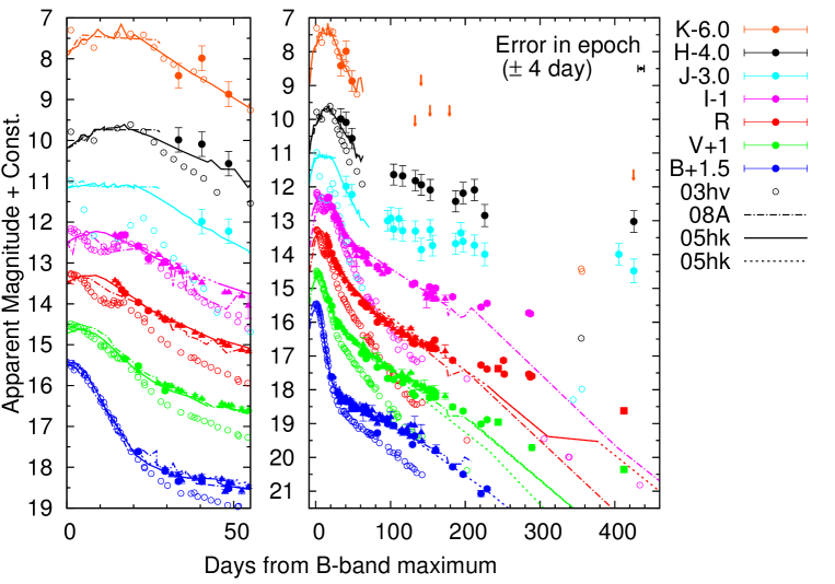
Figure 3: Multi-band light curves of SN 2014dt. The filled circles, triangles and squares denote data that were obtained at Kanata, OKU, and Subaru, respectively. The light curve of each band is shifted vertically as indicated in the top-right portion of the panel. We adopted MJD $56950.4\pm 4.0$ as 0 day, and show its uncertainty in the panel (see §3.3). In the left panel, we show the enlarged ones for the early phase ($\lesssim$ 60 days). For comparison, we show the light curves of SN Iax 2005hk with solid lines (or dashed ones in cases where separation to the neighboring point is $\gtrsim$ 100 days) ($BVRIJHKs$-bands and $F606W$-band; Phillips et al. 2007, Sahu et al. 2008, Friedman et al. 2015, McCully et al. 2010, Stritzinger et al. 2015, Krisciunas et al. 2017) and SN 2008A ($BVRI$, $r^{\prime}i^{\prime}$ and $F555W,F622W,F625W,F791W,F775W$-bands) with dashed-dotted lines (McCully et al. 2010, Hicken et al. 2012, Silverman et al. 2012, Brown et al. 2014, Friedman et al. 2015) and SN Ia 2003hv with the open circles (Leloudas et al.2009).

We compared the long-term decline rates of SN 2014dt at different epochs with those of SNe 2001el (Krisciunas et al. 2003; Stritzinger et al. 2007) and 2003hv (Leloudas et al. 2009), which are well-observed, non-dust forming normal SNe Ia with available late phase optical-NIR photometric data. Figure 4 shows the relationship between the long-term decline rates in optical and NIR bands for SN 2014dt at three epochs, and for SNe 2001el and 2003hv at two epochs. They are well aligned along straight lines, $m_{\rm NIR}$/$m_{\rm opt}\simeq 0.5$–$0.9$, suggesting that the declining trends in optical and NIR wavelengths are similar in those SNe. This suggests that the slow $V$-band decay traces a slow evolution in the bolometric light curves, and it is not caused by a color evolution.

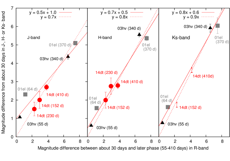
Figure 4: Relationship between the long-term decline rates in the optical and NIR bands for SN 2014dt. The decline rate is measured from $\sim$ 30 days to a given epoch (152, 230 and 410 days) in the late phase. The epochs, as measured from the maximum light, are plotted in parentheses in the figure. For comparison, we plotted those of normal, non-dust forming SN Ia 2003hv at 55 and 340 days as black symbols (Leloudas et al. 2009) and SN 2001el at 64 and 370 days as gray symbols (Krisciunas et al. 2003, Stritzinger et al. 2007). The circle, square and triangle symbols denote data obtained in the $J$, $H$, and $K_{s}$-bands, respectively. The data points were approximately aligned along straight lines suggesting that the long-term decline is homogeneous over optical and NIR bands and that no clear sign of NIR excess was found in SN 2014dt at $230$–$410$ days when the MIR excess was observed (see §4.1).

3.2 Spectral Evolution

Figure 5 shows optical spectra of SN 2014dt from 21 days through 412 days. The early phase spectra are characterized by absorption lines of Na i D, Fe ii, Co ii, and the Ca ii IR triplet (Branch et al. 2004; Jha et al. 2006; Sahu et al. 2008). The line identification is partly in debate due to non-negligible line blending (see below). The line of Si ii $\lambda$6355 is likely hidden by that of Fe ii $\lambda$6456 at 21 days. These lines are usually seen in SNe Iax at similar epochs. The spectral features of SN 2014dt at $21$–$64$ days closely resemble those of SN 2005hk at similar epochs, except that the line width (and the blueshift) of each absorption feature in SN 2014dt is slightly narrower (and smaller) than those in SN 2005hk. This suggests that SN 2014dt had a smaller expansion velocity in the early phase. In Figure 6, we compare the line velocities of Fe ii $\lambda$6149 and $\lambda$6247 lines in SN 2014dt with those in other SNe Iax. We measured the velocities by a Gaussian fit to each absorption line. In each spectrum, we measured it multiple times for each lines. The scatter of the line velocities due to the measurements $\sim$400 km s^-1. The derived velocity was roughly 4000 km s^-1 at $21$ days and decreased to $2000$–$3000$ km s^-1 at $100$–$120$ days. This is slower than those of SNe 2002cx, 2005hk and 2012Z, whereas it is slightly faster than those of SNe 2009ku (Narayan et al. 2011) and 2014ck (Tomasella et al. 2016).

Here, we should be careful in the treatment of line velocities, because the spectra of SNe Iax show many intermediate-mass and Fe-group elements, and it is thus difficult to identify individual lines (e.g., Szalai et al. 2015) even with the less line blending due to the slower expansion than normal SNe Ia. We synthesized model spectra using SYN++ code (Thomas et al. 2011) to provide reliable line identifications. The synthetic spectrum explained the overall features well in the spectrum (Figure 7). At around 6000 Å , the spectral lines of Fe ii likely dominate the observed features, and Fe ii $\lambda$6149 and $\lambda$6247 suffered from little contamination by other lines (e.g., Co ii) as suggested in previous studies (i.e., Stritzinger et al. 2014 for SN 2010ae and Szalai et al. 2015 for SN 2011ay). This supports the idea that the slower expansion of SN 2014dt seen in Figure 6 is real in nature.

In the late phase, 244 and 412 days, the spectra are characterized by many narrow emission lines. Many permitted lines, such as Fe ii, and Ca ii, are seen in addition to forbidden lines, such as [Fe i] $\lambda$7155 and [Ca ii] $\lambda\lambda$7291, 7324. The spectral features at 241 days are still quite similar to those of SN 2005hk at 232 days except for some minor differences, such as the line ratios among emission lines around $8400$–$8700$ Å and the width and blueshift of the Na i D absorption line. Generally, the strength ratio of a forbidden line to a permitted one is an index of the density of the line-emitting region; a smaller ratio indicates a larger density (e.g., Li & McCray 1993). We derived the strength of the emission lines simply by a single-Gaussian fit to each line profile. In the spectrum of SN 2014dt at 244 days, the ratio of [Ca ii] $\lambda\lambda$7291, 7324 to Ca ii $\lambda$8542 was 0.7 $\pm$ 0.1, whereas that in the spectrum of SN 2005hk at 228 days was much larger, 2.5 $\pm$ 0.1. This suggests that the density of the line emitting region in SN 2014dt is higher than that in SN 2005hk.

The spectral evolution through $\simeq 410$ days is markedly different between SNe 2014dt and 2005hk. SN 2014dt showed no significant change except that some Fe ii lines at the shorter wavelengths become weaker. However, in SN 2005hk, the forbidden lines ([Fe i] $\lambda$7155 and [Ca ii] $\lambda\lambda$7291, 7324) become stronger relatively to the continuum and most emission lines become narrower. These indicate that the spectral evolution of SN 2014dt in the late phase was slow, which is likely consistent with the slow decline of the optical and NIR luminosity.

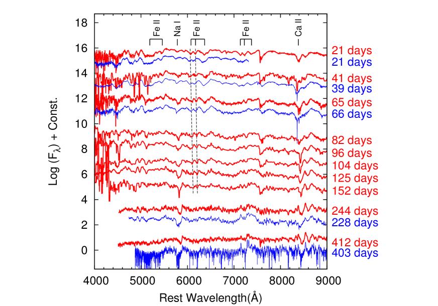
Figure 5: Spectral evolution of SN 2014dt (red solid lines). The epoch of each spectrum is indicated on the right outside the panel. The dashed lines show the positions of Fe ii $\lambda$6149 and $\lambda$6247 lines. For comparison, we plotted the spectra of SN 2005hk (blue lines, Phillips et al. 2007; Blondin et al. 2012; Silverman et al. 2012).

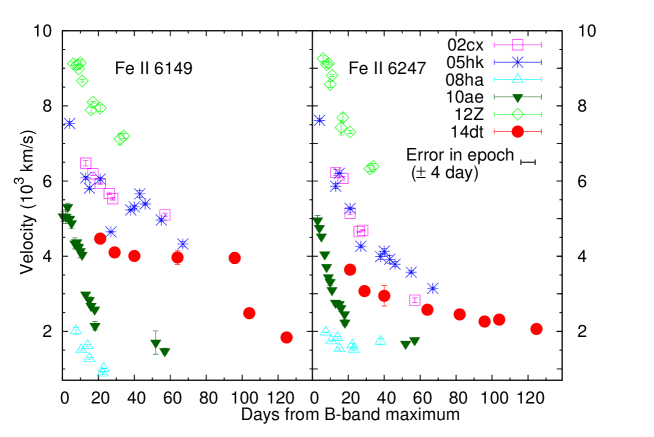
Figure 6: Line velocities of Fe ii $\lambda$6149 and $\lambda$6247 in SN 2014dt. For comparison, we plotted those in SNe Iax 2002cx (Li et al. 2003), 2005hk (Phillips et al. 2007; Blondin et al. 2012; Silverman et al. 2012), 2008ha (Foley et al. 2009; Valenti et al. 2009), 2010ae (Stritzinger et al. 2014) and 2012Z (Stritzinger et al. 2015; Yamanaka et al. 2015). We measured the velocity of the comparison SNe in the same way as for SN 2014dt.

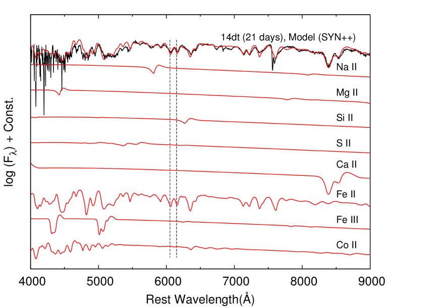
Figure 7: Comparison of the observed spectrum for SN 2014dt at 21 days (black line) and the synthesized spectra calculated with SYN++ code (red lines). We also show the synthesized spectra of each species indicated in the panel. The dashed lines show the positions of Fe ii $\lambda$6149 and $\lambda$6247 lines. It is likely that Fe ii $\lambda$6149 and $\lambda$6247 are little blended with other species (see text).

3.3 Estimation of the Maximum Epoch

It is useful to restrict the epoch of maximum brightness even roughly for comparison with other SNe and theoretical models. We emphasize that the main arguments in this paper are based on the long-term evolution through the late phase, and thus uncertainty in the maximum epoch and explosion date do not alter our main conclusions. However, some of our additional arguments depend on the epoch of maximum brightness. In this subsection, we describe how we estimated the maximum epoch from the observational data of SN 2014dt, for which the maximum date is indeed missing.

Figure 8 shows a spectral comparison of SN 2014dt and other SNe Iax. The spectrum of SN 2014dt on November 10 shows a close resemblance to those of SNe 2002cx at 21 days and 2005hk at 22 days, SN 2012Z at 21 days. The absorption lines of SNe 2008ha and 2010ae are much narrower; however, the overall spectral features are still similar to those of other SNe Iax at similar epochs. This spectral comparison could provide a tentative estimation of the epoch of SN 2014dt: 2014 November 10 was around $21$–$22$ days after the maximum.

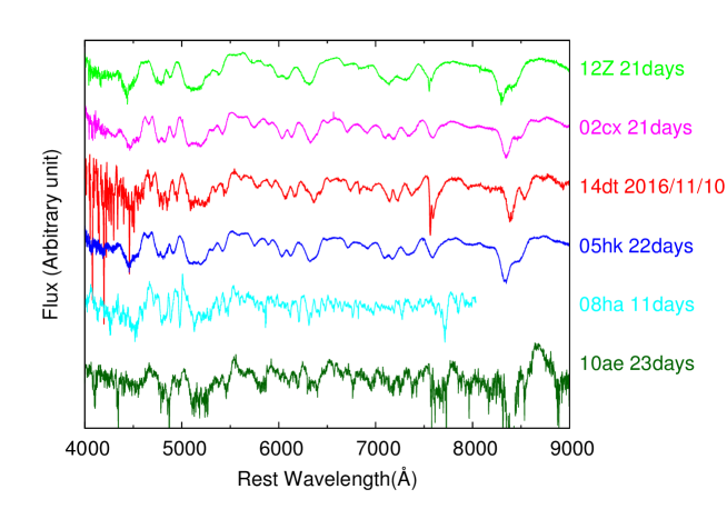
Figure 8: Spectral comparison of SN 2014dt on 2016 November 10 with other SNe Iax; 2012Z (Stritzinger et al. 2015), 2002cx (Li et al. 2003), 2005hk (Blondin et al. 2012), 2008ha (Foley et al. 2009), and 2010ae (Stritzinger et al. 2014). The phase of each spectrum is $\sim$20 days except for SN 2008ha for which no spectrum at $\sim$ 20 days was available.

Next, we considered an estimation of the epoch based on the LCs. Indeed, the multi-band LCs of SN 2014dt apparently closely followed those of SNe 2002cx, 2005hk, and 2012Z in the post-maximum phase, until $\sim 80$ days after the explosion. In this period, the extinction-corrected colors and the spectra of SN 2014dt also resembled those of SNe 2002cx, 2005hk and 2012Z except for a slightly slower expansion velocity (see §3.2). These data allowed us to conclude that the multi-band LCs of SN 2014dt even before the discovery were similar to those of SNe 2002cx, 2005hk and 2012Z. To further quantify the similarity and provide a reasonable estimate on evolution of the LCs of SN 2014dt before the discovery, we examined whether and how the multi-band LCs of these template SNe matched to those of SN 2014dt. The details are given in the Appendix. Here we provide a summary of our analyses.

First, the initial guess in the phase was adopted so that it was 21 days after the maximum on 2014 November 10. For a template LC of each SN in each bandpass, we allowed the shifts along the time axis $\Delta t$ and the magnitude axis $\Delta M$ within given ranges ($|\Delta t|\leq 10$ days and $|\Delta M|\leq 0.3$ mag). For each set of $\Delta t$ and $\Delta M$, we computed a residual between the SN 2014dt and the hypothesized template LC between the discovery date of SN 2014dt and 60 days after the discovery. Then, we estimated the plausible ranges of $\Delta t$ and $\Delta M$ requiring that the residual should be smaller than a given specific value. Performing the same procedure independently for $BVRI$-band LCs, we determined the allowed range of $\Delta t$ and $\Delta M$ so that the fits in all of the bands were mutually consistent. However, we found that the multi-band LCs of SN 2002cx did not provide a consistent solution among different bands; thus we concluded that the LCs of SN 2002cx should be omitted from the template LCs. As a result, we had a series of ‘combined’ LCs for SN 2014dt, in which the pre-discovery part was replaced by the LC of either SN 2005hk or SN 2012Z, taking into account the uncertainty in $\Delta t$ and $\Delta M$. Further details can be found in Appendix. Thus, we derived the epoch of $B$-band maximum as MJD $56950.4\pm 4.0$ (2014 October 20.4 UT), which was in accordance with the results of the spectral comparison and the also with the previous estimate (Foley et al. 2016, Fox et al. 2016 and Singh et al. 2018).

3.4 Maximum Magnitude v.s. Decline Rates

For the ‘combined’ LCs constructed in §3.3 (see also Appendix), we estimated the maximum magnitude and the decline rate, $\Delta m_{15}$, as well as the epoch of the maximum light in each of the $VRI$-bands (Table 5). After correcting the distance modulus and the total extinction (see §1), we derived the absolute maximum magnitude in the $B$-band, $M_{B,{\rm max}}=$ $-16.82$–$-17.34$ mag. It is $\sim$1 mag fainter than that obtained by Singh et al. (2018), which is apparently originated from the systematic difference in the $B$-band magnitude of the companion stars (see §2) and in the adopted distance modulus. Our $M_{B,{\rm max}}$ was slightly ($0.2$–$1.2$ mag) fainter than those of SNe Iax 2002cx ($M_{B,{\rm max}}=-17.55\pm 0.34$ mag; Li et al. 2003), 2005hk ($M_{B,{\rm max}}=-18.02\pm 0.32$ mag; Phillips et al. 2007, $M_{B,{\rm max}}=-18.00\pm 0.25$ mag; Stritzinger et al. 2015), and 2012Z ($M_{B,{\rm max}}=-18.27\pm 0.09$ mag; Stritzinger et al. 2015, $M_{B,{\rm max}}\sim-17.61$ mag; Yamanaka et al. 2015 ), whereas it was $3.1$–$3.6$ mag brighter than that of SN 2008ha ($M_{B,{\rm max}}=-13.74\pm 0.15$ mag; Foley et. al. 2009, $M_{B,{\rm max}}=-13.79\pm 0.14$ mag; Stritzinger et al. 2014). It is noted that this estimate conservatively included the uncertainty in the ‘combined’ LCs in terms of the template LCs (SN 2005hk or SN 2012Z) and the fitting uncertainties in $\Delta t$ and $\Delta M$.

lccc Peak magnitude and its epoch of SN 2014dt in each photometric band Band Maximum date (MJD) Maximum magnitude $\Delta m_{15}$
They are deduced from the light curves combined with those of SNe 2005hk
and 2012Z since the observed light curves of SN 2014dt do not cover the
peak magnitude. See §3.3 for details. Magnitude difference between 0 days and 15 days after the maximum. $B$ 56950.4 $\pm$ 4.0 $13.88$–$13.76$ $1.43$–$1.57$
$V$ 56954.9 $\pm$ 4.0 $13.56$–$13.50$ $0.73$–$0.91$
$R$ 56957.5 $\pm$ 4.0 $13.47$–$13.28$ $0.51$–$0.66$
$I$ 56958.5 $\pm$ 4.0 $13.63$–$13.30$ $0.48$–$0.66$

The derived decline rate of SN 2014dt was $\Delta m_{15}(B)=1.43$–$1.57$ mag. As shown in Table 5, the decline rate was smaller at longer wavelengths. Figure 9 shows the relationship between $M_{V,{\rm max}}$ and $\Delta m_{15}(V)$ in some SNe Iax and normal SNe Ia. SN 2014dt apparently belonged to the group of the bright SNe Iax including SNe 2002cx, 2005hk and 2012Z. From 60 through 410 days, the differences in LCs from those of SN 2005hk became significant (Figure 3); SN 2014dt showed a slower decline than SN 2005hk. This is confirmed in Figure 10 where the ‘long-term decline rates’ ($0$ to $200$–$250$ days) in the $B$-band were plotted. Among three SNe Iax for which $B$-band photometric data at $200$–$250$ days existed SN 2014dt showed the smallest long-term decline rate, and was the smallest compared to larger samples of normal SNe Ia. We found no clear trend between the absolute maximum magnitude and the long-term decline rate among SNe Iax samples or normal SNe Ia samples (see §4. for discussion). The large error in $\Delta m_{200-250}(B)$ stemmed from our conservative error estimated in the maximum magnitude. Indeed, it is clear from Figure 3 that the LCs of SN 2014dt were much flatter in the late phase than those of SN 2005hk (see §3.1).

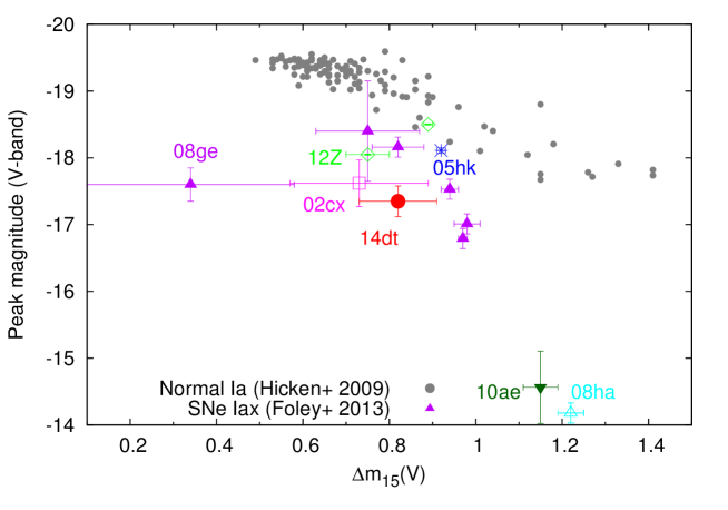
Figure 9: Correlation of the peak absolute magnitudes in the $V$-band with the decline rate $\Delta m_{15}(V)$. The gray filled circles are the data points of normal SNe Ia (Hicken et al. 2009), and the other symbols are for SNe Iax (Li et al. 2003; Foley et al. 2009; Foley et al. 2013; Stritzinger et al. 2014; Stritzinger et al. 2015; Yamanaka et al. 2015). For some SNe Iax, the SN IDs are indicated one by one.

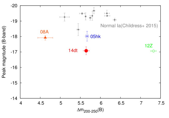
Figure 10: Relationship between the peak absolute magnitudes in the $B$-band and the long-term decline rate; that is, the magnitude difference between $0$ and $200$–$250$ days after the maximum light (see §3.4), in the $B$-band. The data for normal SNe Ia are from Childress et al. (2015).

3.5 Spectral Energy Distribution

Our observations may provide the first opportunity to examine the long-term, optical and NIR multi-band photometry for SNe Iax, which enables studying the evolution of SED through the late phase, including any possible contribution from circumstellar (CS) dust. At longer wavelengths, Fox et al. (2016) reported that SN 2014dt showed brightening around 300 days at mid-infrared (MIR) wavelengths and suggested that thermal emissions from pre-existing dust grains could cause MIR excess.

We derived SEDs of SN 2014dt by combining the optical and NIR photometric data at similar epochs (difference $\lesssim$ 14 days), and plotted them in Figure 11 together with representative blackbody (BB) spectra. The BB temperature is roughly an indicator of the photospheric temperature. Initially (between 40 days and 132 days) the BB temperature seemed to decrease rapidly from $\sim 5000$ K to $\sim 3700$ K, but thereafter the BB temperature showed no significant change through 410 days, whereas the peak flux gradually decreased. For some SNe Iax, McCully et al. (2014) points out that temperature evolution obtained by the ratio of the permitted Ca ii lines is slower than $t^{-1}$ or even constant. This might be commonly seen in SNe Iax. However, the fluence ($\lambda F_{\lambda}$) at MIR wavelengths gradually increased during the period of $309$–$336$ days (Fox et al. 2016), although it was still much smaller than those in optical and NIR wavelengths. The spectral slope of the MIR excess was inconsistent with the main SED component peak at optical wavelengths, and thus the MIR excess would only represent a minor, additional component.

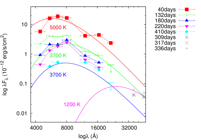
Figure 11: The evolution of the SED of SN 2014dt. For data at 180, 220, and 410 days, we plotted the combined data at similar epochs (difference $\lesssim$ 14 days) because we did not always have the data exactly at the same epoch. The data at mid-infrared wavelengths (the gray points) are from Fox et al. (2016). For comparison, we plotted the blackbody spectra for 5000, 3700, and 1200 K by the solid lines.

4 Discussion

4.1 Interpretation of the SED Evolution

As shown in Figure 11, the main SED component ($\sim 3700$ K BB emission) dominated the optical and NIR flux from 180 days to 410 days. This long-lasting SED component could be an analog to the component that Foley et al. (2016) found for SN 2005hk by continuum fits to late phase spectra. The authors suggested that the long-lasting photospheric emission could have originated in a wind launched from a bound remnant in a context of the weak deflagration model. It is plausible that this photospheric emission component corresponded to the main SED component derived for SN 2014dt.

The combination of the bolometric luminosity and the temperature obtained through the SED fitting suggests that the photosphere is located at $R_{\rm ph}\sim 6.2\times 10^{14}$ cm at 230 days. Assuming that the bolometric luminosity follows the ⁵⁶Co decay, then the nearly unchanged temperature suggests $R_{\rm ph}\sim 2.9\times 10^{14}$ cm at 410 days, i.e., the photospheric radius has decreased by about a factor of two from 230 days to 410 days. Assuming that the opacity is $0.1$ cm² g^-1, then $R_{\rm ph}$ (230 days) suggests that $\sim 8\times 10^{-3}M_{\odot}$ of the material is confined within this radius. If the photosphere could be located within the homologously expanding inner ejecta, then the corresponding velocity is $\sim 300$ km s^-1 and $\sim 80$ km s^-1 at 230 and 410 days, respectively. To compare to these values of the velocity, the late phase spectra at 232 and 412 days show some permitted lines whose widths are marginally resolved by our spectroscopic observations. Given the resolution of 650, the velocities of these permitted lines should be an order of 100 km s^-1, while the precise measurement is not possible. In the discussion below, we just use the rough value (a few 100 km s^-1) in a qualitative way.

The photospheric radius far exceeds the size of a red supergiant, and therefore it is unlikely that this is created by a (nearly hydrostatic) atmosphere of a hot (remnant) white dwarf within the weak deflagration scenario. The overall feature may be consistent with a scenario that the photosphere is located deep in the homologously expanding ejecta, as the inferred velocity is consistent with those measured in the spectra but within the spectral resolution. Indeed, Foley et al. (2016) argued against this interpretation the photosphere in the ejecta for SN 2005hk, by pointing out the discrepancy (in a snapshot spectrum) in the velocities measured in these two different approach. If the photosphere is in the homologously expanding ejecta, it predicts that the associated line velocity decreases as time goes by (see above, i.e., by a factor of nearly 4 from 200 to 400 days), and thus an accurate measurement of the line velocities and their evolution is a key in testing this scenario with the photosphere located deep in the ejecta. This scenario on the other hand naturally explains the decrease in the photospheric radius, as the density of the emitting material decreases.

Alternatively, the photosphere might have formed within a wind lunched by the possible bound remnant white dwarf, as suggested by Foley et al. (2016) for SN 2005hk. In this case, a line velocity has no direct link to the photospheric radius but determined by the velocity of the wind. Still, it should be an order of at least $100$ km s^-1 to create the photosphere at $R>10^{14}$ cm. The mass within the photosphere ($\sim 8\times 10^{-3}M_{\odot}$ as measured at 230 days) is translated to the wind mass loss rate of $\sim 10^{-2}M_{\odot}$ yr^-1, and the kinetic power of $\sim 3\times 10^{37}$ erg s^-1 to $10^{39}$ erg s^-1 for the wind velocity of $\sim 100-1000$ km s^-1. This is roughly the Eddington luminosity for the expected bound remnant, thus is in line with the wind scenario. A possible drawback of the wind scenario is that there is no obvious reason about why the photosphere radius has been decreased, as the ‘stationary wind’ would not provide a change in the density scale to change the position of the photosphere.

In summary, it is not possible to make a strong conclusion on the origin of the photospheric component. Both of the ejecta model and the wind model have advantage and disadvantage. In any case, we add several new constraints on the nature of this emission to the suggestion by Foley et al. (2016); for example, any model should explain the recession of the photosphere, and the mass of the material must be at least $\sim 10^{-3}M_{\odot}$. In either case, the need of the high-density material in the inner part of the ejecta could support the weak deflagration scenario and the existence of the bound remnant.

4.2 Interpretation of the MIR Excess

Here we briefly discuss the origin of the minor MIR excess (§3.5). Foley et al. (2016) suggested that the emissions from circumstellar dust seemed unlikely, because neither additional reddening nor narrow absorption lines due to a possible circumstellar interaction has been observed in late phase optical spectra of SNe Iax. They further argued against thermal emissions from newly formed dust grains within the ejecta, based on the lack of expected signatures such as the blueward shift of the spectral lines and additional reddening. Alternatively, the authors suggested that the emissions from a bound remnant with a super-Eddington wind were plausible as a source of the MIR excess. However, as shown above, the main component that we derived for SN 2014dt was indeed an analog to what Foley et al. (2016) suggested for SN 2005hk, representing a possible bound remnant. By this component alone, it is hard to explain the MIR excess.

Thus, we speculate that an echo by circumstellar material (CSM) is the most likely interpretation of the MIR excess. This would not contradict the lack of strong extinction and narrow emission lines. For example, the CSM of the over-luminous SN Ia 2012dn is likely to be located off the line of sight, and the separation between the CSM and the SN is too far to allow a strong interaction within the first few years after the explosion (Yamanaka et al. 2016, Nagao et al. 2017). A similar configuration may apply to the case of SN 2014dt.

As mentioned in §3.5, the MIR excess only provided a minor contribution to the SED. However, it may not be negligible in the $K_{s}$-band at 410 days if the continuum from a hot dust ($\sim 1200$ K) is the origin of the MIR excess and it may contaminate the NIR fluxes (see Figure 11). Thus, it is interesting to check for possible contamination in our NIR data. If the possible additional component to the intrinsic SN emission in the NIR bands exists, the data point should be significantly lower than the straight lines in Figure 4 (see §3.1). Thus, we exclude the existence of the additional component in the NIR bands, and the dust should not be hot (i.e., $\lesssim 1200$ K) if thermal emissions from dust is the origin of the MIR excess.

4.3 Two-component fit to the bolometric LC: A support to the weak deflagration model with a bound remnant

We derived the bolometric luminosity of SN 2014dt assuming that the sum of fluxes in the $BVRI$-bands occupied about 60 % of the bolometric one (Wang et al. 2009). The derived bolometric LC is shown in Figure 12, which is one of the ‘combined LCs’, with the template LCs taken from SN 2005hk and $\Delta t=0$ days (see §3.3 and Appendix). In the early phase, SN 2014dt was $0.1$–$0.5$ dex fainter than SNe 2002cx, 2005hk, and 2012Z. SN 2014dt showed a significantly slow decline after $\sim 60$ days, and then its luminosity became comparable with that of SN 2005hk as well as $\sim 0.5$ dex brighter than that of SN 2012Z at $230$–$250$ days. With the peak luminosity ($L_{\rm bol,max}$) and rising time ($t_{r}$), we could estimate the mass of the synthesized ⁵⁶Ni (Arnett 1982; Stritzinger & Leibundgut 2005). The rising part of the LC in SN 2014dt was not observed. SNe Iax show larger diversity, but it is pointed out that the rise time of SNe Iax has a correlation with the peak magnitude (Magee et al. 2016). SN 2014dt is slightly fainter than SNe 2005hk and 2012Z, and it might be not a clear outlier like SN 2007qd (McClelland et al. 2010, Magee et al. 2016). We assume that the rise time of SN 2014dt is roughly similar to the rise time of SNe 2005hk and 2012Z. Adopting SN 2005hk and 2012Z as a template, we tested a range of rising times to estimate the mass of ⁵⁶Ni. The definition of the rising time can differ in different literatures, so we decided to derive the rising time ourselves. We fitted each of the multi-band LCs of SNe 2005hk and 2012Z by a quadratic function, deriving rising times, and $t_{r}=16.5$–$21.0$ and $11.8$–$12.8$ days for SNe 2005hk and 2012Z, respectively, which are consistent with those in previous papers. Using $L_{\rm bol,max}=$ ($1.2$–$1.8$) $\times 10^{42}$ erg s^-1 and $t_{r}=11.8$–$21.0$ days, we estimated the ⁵⁶Ni mass as $0.04$–$0.10$M_⊙ for SN 2014dt. It unfortunately has a large uncertainty, because the data around the maximum light are missing for SN 2014dt.

We also estimated the ⁵⁶Ni mass from the late phase bolometric LC, which was subject to much less contamination by the error of the explosion epoch. First, we estimated the ⁵⁶Ni mass by a fit of a simple radioactive-decay LC model in the late phase (e.g., Maeda et al. 2003),

$$L_{\rm bol} = M(^{56}$$ Ni) [ e^(-t/8.8 d) ϵ_γ,Ni (1 - e^-τ) (1)

$$+\left.e^{(-t/113{\rm\ d})}\left\{\epsilon_{\gamma,\rm Co}(1-e^{-\tau})+\epsilon_{e^{+}}\right\}\right]$$, and

$$\tau\simeq 1000\times\left[\frac{(M_{\rm ej}/M_{\odot})^{2}}{E_{51}}\right](t\mbox{day})^{-2}\mbox{ ,}$$ (2)

where $\epsilon_{\gamma,\rm Ni}=3.9\times 10^{10}$ erg s^-1 g^-1 is the energy deposition rate by ⁵⁶Ni via $\gamma$-rays, $\epsilon_{\gamma,\rm Co}=6.8\times 10^{9}$ erg s^-1 g^-1 and $\epsilon_{e^{+}}=2.4\times 10^{8}$ erg s^-1 g^-1 are those by the ⁵⁶Co decay via $\gamma$-rays and positron ejection, $M_{\rm ej}$ is the ejecta mass, and $E_{51}$ is the kinetic energy of $10^{51}$ erg. However, it does not consistently explain the derived bolometric LC at both and early and late phases. The slow tail in the obtained bolometric LC of SN 2014dt after $\sim 60$ days required nearly a full trapping of the deposited energy (that is, a larger $\tau$). However, the full trapping of $\gamma$-rays with $\sim 0.10$ M_⊙ of ⁵⁶Ni / ⁵⁶Co (as derived above to fit the peak) should result in a much larger $L_{\rm bol}$ in the late phase (see Figure12).

Thus, we adopted a two-component LC model (Maeda et al. 2003) where $L_{\rm bol}$ is a sum of $L_{\rm bol,in}$ and $L_{\rm bol,out}$. In this model, we have four independent parameters in total, $M_{\rm in}(^{56}$Ni$),[(M_{\rm ej}/M_{\odot})^{2}/E_{51}]_{\rm in}$, $M_{\rm out}(^{56}$Ni$)$ and $[(M_{\rm ej}/M_{\odot})^{2}/E_{51}]_{\rm out}$. The former two parameters (subscripted by ‘in’) correspond to an inner, larger $\tau$ component, and the latter two correspond to the outer, smaller $\tau$ one. With this model, we successfully reproduced the LC which well traces the bolometric LC from near maximum to $\sim 250$ days as shown in Figure 12.

The parameters obtained by the fit were $M_{\rm in}(^{56}$Ni$)=$ $0.015$–$0.025$ M_⊙, $[(M_{\rm ej}/M_{\odot})^{2}/E_{51}]_{\rm in}\gtrsim 500$, $M_{\rm out}(^{56}$Ni$)=$ $0.02$–$0.08$ M_⊙ and $[(M_{\rm ej}/M_{\odot})^{2}/E_{51}]_{\rm out}\sim$ $0.8$–$3.0$. Again, we noted that the errors were conservatively associated with a series of the allowed combined LCs for SN 2014dt (§3.3), which is also the case for the following analyses. We could only estimate a rough lower-limit for $[(M_{\rm ej}/M_{\odot})^{2}/E_{51}]_{\rm in}$ so that it was large enough to fully trap the $\gamma$-rays even at $250$–$410$ days. That is, the need for the high-density inner component was robust and insensitive to the parameters for fit. At 410 days, the bolometric LC of SN 2014dt was slightly brighter than the two-component model LC. Contamination by the galaxy background was small in this phase (see Foley et al. 2014). If this excess was real, one possible explanation is the contribution from a scattering component of a presumed CSM echo, corresponding to the MIR excess (§4.1).

The existence of the large $\tau_{\rm in}$ component suggests that there is an inner component that keeps a high density even in the late phase, regardless of the origin (see §4.1). This is consistent with the prediction of the weak deflagration model with a bound remnant (e.g., Fink et al. 2014).

4.4 Properties of Ejecta

In the two-component model, the inner, dense component may be connected with the existence of a bound white dwarf, and the outer, less dense one may correspond to the SN ejecta. Assuming that the outer component ($[(M_{\rm ej}/M_{\odot})^{2}/E_{51}]_{\rm out}\sim$ $0.8$–$3.0$) was the main ejecta, we could estimate $M_{\rm ej}$ and $E_{\rm k}$ of the ejecta in SN 2014dt by applying the scaling laws,

$$t_{\rm d}\propto\kappa^{1/2}\ M_{\rm ej}^{3/4}\ E_{\rm k}^{-1/4}\mbox{, and}$$ (3)

$$v\propto E_{\rm k}^{1/2}\ M_{\rm ej}^{-1/2}\mbox{,}$$ (4)

calibrated with the well-studied SNe Ia, where $t_{\rm d}$ is the diffusion timescale, $\kappa$ is the absorption coefficient for optical photons, and $v$ is the typical expansion velocity of the ejecta. Here, we adopted the parameters derived for SN Ia 2011fe (Pereira et al. 2013) for the normalization. From Equations (3) and (4), we obtained the following equations of the ratios in $M_{\rm ej}$ and $E_{\rm k}$,

$$\frac{M_{\rm ej,14dt}}{M_{\rm ej,11fe}}=\left(\frac{t_{\rm d,14dt}}{t_{\rm d,11fe}}\right)^{2}\times\frac{v_{\rm 14dt}}{v_{\rm 11fe}}\times\frac{\kappa_{\rm 11fe}}{\kappa_{\rm 14dt}}\mbox{, and}$$ (5)

$$\frac{E_{\rm k,14dt}}{E_{\rm k,11fe}}=\left(\frac{t_{\rm d,14dt}}{t_{\rm d,11fe}}\right)^{2}\times\left(\frac{v_{\rm 14dt}}{v_{\rm 11fe}}\right)^{3}\times\frac{\kappa_{\rm 11fe}}{\kappa_{\rm 14dt}}\mbox{.}$$ (6)

The expansion velocity of a SN Ia is usually estimated from the blueshift of the Si ii $\lambda$6355 absorption line at $\sim 0$ day (e.g., $v_{\rm 11fe}\simeq 10500$ km s^-1; Pereira et al. 2013). The Si ii $\lambda$6355 absorption line of SN Ia is strong at $\sim 0$ day and is little contaminated by other absorption lines (e.g, SN 2011fe; Parrent et al. 2012). However, we have no spectrum of SN 2014dt around the maximum. In addition, it is often difficult to identify the Si ii $\lambda$6355 line in the spectra of SNe Iax at 10 days and later. Thus, we estimated the Si ii $\lambda$6355 line velocity, assuming that the ratio between the velocity of Si ii $\lambda$6355 at $\sim 0$ day and that of Fe ii lines velocity at $\sim 20$ days was similar among SNe Iax samples (i.e., SNe 2005hk, 2012Z and 2014dt). In SNe Iax, the Fe ii $\lambda$6149 and $\lambda$6247 lines were not much blended (see §3.2). In this way, we estimated $v_{\rm 14dt}=3500$–$4200$ km s^-1.

The diffusion timescale, $t_{\rm d}$, approximately corresponds to the width of the peak in the bolometric LC. We derived the ratio of $t_{\rm d,14dt}/t_{\rm d,11fe}$ as $1.0$–$1.6$, by comparing the durations for the two SNe from the maximum to the epoch when the magnitude decreased by 0.5 dex.

For $\kappa$, it would not be safe to simply assume that the opacity of SN 2014dt is the same as that of SN 2011fe, because the properties of SN ejecta would be considerably different between SNe Iax and normal SNe Ia (i.e., $\kappa_{\rm 14dt}\neq\kappa_{\rm 11fe}$). Thus, we kept it as a free parameter and added another observational constraint using the post-maximum LC, when the LC is still dominated by the ejecta (that is, the outer component). With $E_{\rm k,11fe}=1.2\times 10^{51}$ erg (Pereira et al. 2013) and $M_{\rm ej,11fe}=1.4$ M_⊙, we obtained $E_{\rm k,14dt}=$ ($0.07$–$0.42$) $\times 10^{50}$ erg, $M_{\rm ej,14dt}=0.08$–$0.35$ M_⊙ and $\kappa_{\rm 14dt}/\kappa_{\rm 11fe}=1.5$–$11.6$. The relatively large uncertainties reflect the large errors in the estimated explosion epoch (see §3.4). Similarly, we obtained $\kappa_{\rm 05hk}/\kappa_{\rm 11fe}=2.2$–$4.3$ (see §4.5 for details). Interestingly, the opacity of the SNe Iax was found to be larger than that of normal SNe Ia. Foley et al. (2013) found the ejecta mass of SNe Iax is systematically small based on the LC analysis . The contribution of the iron-group elements to the opacity could differ from those in the ejecta of normal SNe Ia. This large ratio $\kappa_{\rm Iax}/\kappa_{\rm 11fe}$ indicates that a difference exists. However, for a more realistic treatment, one has to take into account the different physical properties (e.g., ionization) in SNe Iax and normal SNe Ia, which is beyond the scope of this study.

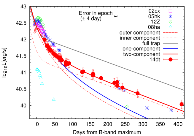
Figure 12: The bolometric light curve of SN 2014dt. This is the ‘combined’ bolometric LC with the template LCs taken from SN 2005hk and $\Delta t=0$ days (see §4.2 and Appendix). The red filled and open circles are the bolometric luminosities obtained from the sum of fluxes in the $BVRI$-bands and those from fitted template LCs in SN 2005hk, respectively. At 232, 287 and 412 days, we calculated the bolometric luminosity from only $V$- and $R$-band fluxes under the assumption of the non-evolving SED shape at $\gtrsim 100$ days (see §3.5) because we did not have $B$- and $I$-band data. For comparison, we plotted the LCs of SNe 2002cx (Li et al. 2003), 2005hk (Sahu et al. 2008), 2008ha (Foley et al. 2009) and 2012Z (Yamanaka et al. 2015). The gray, blue and red solid lines show the full-trap model, and one- and two-component LC models, respectively. In these models, the total ⁵⁶Ni mass is set to be $\sim$0.10 M_⊙. The dashed and dotted lines indicate the outer and inner components, respectively, in the two-component model.

4.5 Explosion Mechanism

We discuss the explosion mechanism of SN 2014dt based on the explosion parameters derived above. Since the derived explosion parameters have a large uncertainty, the discussion here should be regarded as being qualitative. For SNe Iax, several different explosion models have been suggested (e.g., the weak deflagration model with or without a bound remnant, the pulsating delayed detonation, and the fallback CC models). For the weak deflagration model without a bound remnant (Nomoto et al. 1976; Branch et al. 2004; Jha et al. 2006; Sahu et al. 2008), our analysis suggests that this model clould not explain the slow decline LC in the late phase (see §4.2). As previously mentioned, the observational properties of SNe Iax are explained by the pulsational delayed detonation model (PDD model; Höeflich et al. 1995, Höeflich & Khokhlov 1996) (e.g., SN 2012Z; Stritzinger et al. 2015). In the PDD model, the detonation is triggered after the deflagration phase. This creates a high-density inner ejecta, and thus it may explain the slow evolution and low velocities seen in the late time spectra of SN 2014dt.

In Table 6, we show the characteristic explosion parameters predicted by the weak deflagration model with a bound remnant (Fink et al. 2014) and by the fallback CC SN model (Moriya et al. 2010), which are apparently consistent with those derived for SN 2014dt. In the fallback CC model, some progenitor models (a He star with initial mass of $40$ M_⊙, CO stars with initial masses of $25$ and $40$ M_⊙) seem to explain the observations. However, Foley et al. (2015) gave the upper-limit of the brightness of the progenitor from the pre-explosion images taken by the HST and suggested that an existence of a massive star in the progenitor system is unlikely. Thus, we consider that the weak deflagration model with a bound remnant is most plausible for SN 2014dt. However, the explosion parameters of SN 2014dt have large uncertainties due to a lack of pre-maximum data. Thus, we do not argue strongly that the derived parameters provide a strong evidence of the weak deflagration scenario. Rather, we list this analysis as a supporting evidence to the arguments in the late phase behaviors, which led us to suggest the weak deflagration model for SNe 2014dt and 2005hk. The slow evolution in the SED of SN 2014dt in the same phase (§4.1) seems consistent with this model.

Our late time data revealed the nearly unchanged SED and full $\gamma$-ray trapping, which are difficult to explain by the expanding SN ejecta with decreasing density. It is thus tempting to connect these properties to the weak deflagration model, in which the bound remnant and its atmosphere may serve as a high-density “stationary” source of the energy input. If the PDD model would also create a slow, high-density Fe-rich ejecta which keeps opaque for 400 days, this could also be a viable model, while this may require fine-tuning in the model. We suggest the weak deflagration as a straightforward interpretation, but distinguishing these two scenarios will require further study both in theory and model. Indeed, there are two possible drawbacks so far raised for the weak deflagration model. (1) The weak deflagration model by Fink et al. (2014) leads to a rapid decline in the post-maximum phase. However, the model does not include the effect of the central remnant, and thus the investigation of the effects of the bound remnant in the LC is strongly encouraged. (2) The weak deflagration model inevitably leads to a well-mixed, non-stratified structure in the ejecta, while the layered structure has been inferred at least for some SNe Iax from the velocity evolution (SN 2012Z; Stritzinger et al. 2015) and through spectral modeling (SN 2011ay; Barna et al. 2017). Indeed, this feature has been suggested to be consistent with the PDD model rather than the weak deflagration model (Stritzinger et al. 2015). To further add possible diagnostics to differentiate the two models, we encourage to investigate the evolution of line velocities in the late phase. The two scenarios may predict the difference in the formation of the low velocity permitted lines in the late phase. The weak deflagration model could produce them either in the remnant WD and the slow expanding ejecta, while only the latter is possible in the PDD. As these two mechanism will lead to different evolution in the line velocities, a high-resolution spectroscopy in the late phase may solve this issue.

lccc Comparison of explosion parameters with candidate models Model Explosion energy ($10^{50}$erg) Ejecta mass ($M_{\odot}$) ⁵⁶Ni mass ($M_{\odot}$)
With a bound remnant. N1def and N3def models for Fink et al. (2014) He star with initial mass of 40 M_⊙, CO stars with initial masses of $25,40$ M_⊙ for Moriya et al. (2010) This study. ⁵⁶Ni mass of SN 2005hk is referred to Sahu et al. (2008). Weak deflagration $0.149$–$0.439$ $0.0843$–$0.195$ $0.0345$–$0.0730$
Core collapse (40He) $0.12$–$0.33$ $0.10$–$0.23$ -
Core collapse (25CO) $0.073$–$0.33$ $0.056$–$0.24$ -
Core collapse (40CO) $0.038$–$0.39$ $0.029$–$0.25$ -
SN 2014dt $0.07$–$0.42$ $0.08$–$0.35$ $0.04$–$0.10$
SN 2005hk $0.42$–$0.88$ $0.21$–$0.42$ $0.17\pm 0.02$

4.6 Comparison with another SN Iax 2005hk

It is interesting seen in discuss the diversities in the observed properties of SNe Iax 2005hk, 2012Z and 2014dt from a viewpoint of the prediction of the weak deflagration model. As shown in §3, the diversities in photometric and spectroscopic data are likely more significant in the late phase than in the early phase. In this subsection we apply the modeling procedure adopted in the previous sections to another SN Iax 2005hk, to investigate whether SN 2005hk can be explained within the same context of the weak deflagration model.

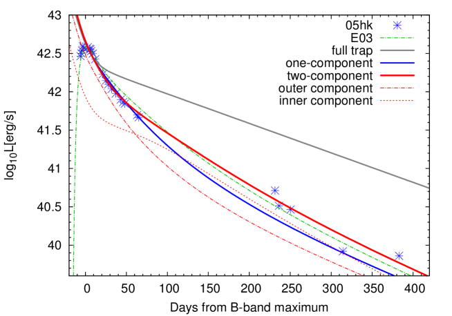
Figure 13: The bolometric light curve of SN 2005hk and corresponding LC models. The lines are plotted in the same manner as in Figure 12. The total ⁵⁶Ni mass is 0.18 M_⊙. We also plotted the LC of the E03 model (weak deflagration model without a bound remnant; Sahu et al. 2008) by a green dashed line (see §4.5), which also well represents the entire LC from the early through the late phases.

For SN 2005hk, Sahu et al. (2008) suggested the weak deflagration model without a bound remnant, which could reproduce the LC. The LC model ‘E03’ in Figure 11 is the LC presented by Sahu et al. (2008), where the explosion parameters are $E_{\rm k,05hk}=3.0\times 10^{50}$ erg and $M_{\rm ej,05hk}=1.4$ M_⊙. In the sequence of the weak deflagration models by Fink et al. (2014), it is expected that such a small $E_{\rm k}$ model would leave a bound remnant. The critical value is $\sim$($6.0$–$7.0$) $\times 10^{50}$ erg (Fink et al. 2014). However, considering the uncertainty in the model, it is difficult to conclude that kinetic energy as small as $3.0\times 10^{50}$ erg should be associated with a bound remnant.

Alternatively, a two-component model can also explain the LC of SN 2005hk, which mimics the presence of a bound remnant (Figure 13). The parameters of the two-component model are $M_{\rm in}(^{56}$Ni$)\sim 0.04$ M_⊙, $[(M_{\rm ej}/M_{\odot})^{2}/E_{51}]_{\rm in}\sim 30$, $M_{\rm out}(^{56}$Ni$)\sim 0.14$ M_⊙ and $[(M_{\rm ej}/M_{\odot})^{2}/E_{51}]_{\rm out}\sim 1.0$–$2.0$. SN 2005hk has a smaller fraction of the ⁵⁶Ni mass in the inner component than SN 2014dt. In the same way, we estimated the explosion parameters for SN 2005hk as $E_{\rm k,05hk}=$($0.42$–$0.88$) $\times 10^{50}$ erg and $M_{\rm ej,05hk}=0.21$–$0.42$ M_⊙ within the context of the two-component model. The derived $[(M_{\rm ej}/M_{\odot})^{2}/E_{51}]_{\rm in}$ indicates that the average density in the inner component of SN 2014dt may be larger than that of SN 2005hk, consistent with indications from the late phase spectra (§3.2). The $E_{\rm k,05hk}$ and $M_{\rm ej,05hk}$ are consistent with the weak deflagration model with a bound remnant, whose mass is smaller than in SN 2014dt (Fink et al. 2014).

In summary, we conclude that SN 2005hk can be explained by the weak deflagration model as well. It is unclear whether SN 2005hk left a bound remnant. If a bound remnant was left, the mass of the remnant would be smaller than in SN 2014dt.

5 Conclusions

We presented long-term optical and NIR observations of SN 2014dt up to 410 days after the maximum light. The data for SNe Iax in the NIR bands are rare, especially in the late phase. We could obtain the NIR evolution for SN 2014dt until the late phase. The LC showed a considerably slow decline in the late phase; the decline rate was the smallest among well-studied SNe Iax samples. From the evolution of the SED, SN 2014dt did not show significant change in the BB temperature. The spectral features were also slow in SN 2014dt in the late phase. A bound remnant left after the explosion gives a good account of these observational properties.

By scaling the explosion parameters of normal SN Ia 2011fe, we suggest that the mass of synthesized ⁵⁶Ni was $0.04$–$0.10$ M_⊙, the kinetic energy was ($0.07$–$0.42$) $\times 10^{50}$ erg, and the ejecta mass was $M_{\rm ej}=0.08$–$0.35$ M_⊙. These values are consistent with the prediction of the weak deflagration model with a bound remnant. However, the uncertainties in the derived explosion parameters for SN 2014dt were large, reflecting our conservative error estimation associated with a possible range of the missed pre-maximum LC behavior.

In summary, the overall properties derived from the long-term observations of SN 2014dt could be explained with the weak deflagration model, with leaves a bound remnant after the explosion. Indeed, by applying the same model to SN 2005hk, we found that SN 2005hk could also be explained by the weak deflagration model with an explosion energy larger than for SN 2014dt. With the larger kinetic energy, it might not leave a bound remnant. The present work demonstrates the power and importance of late phase observations to uncover the origin of SNe Iax. To further test the explosion models, we need to obtain a larger sample of well-observed SNe Iax in the future.

While the weak deflagration model with the bound remnant provides straightforward interpretation to our data, further study is required to robustly identify the explosion mechanism. For example, the PDD model may also account for main observational features including those derived from our data set. For example, further study on the predicted observable based on large model grids both for the deflagration and PDD scenarios will help to resolve the issue, including the synthetic light curves for the deflagration model including the contribution from the bound remnant. Observationally, a key would be high spectral-resolution observations in the late phase to robustly measure the velocities of the low velocity permitted lines and their evolution, which would be used to identify the origin of the late phase slow evolution in the SED either as being caused by the low velocity ejecta or the WD wind.

Appendix A Estimate of the Pre-maximum LC Behavior

Here we describe how to constrain the maximum brightness and the maximum date of SN 2014dt. We compared its early multi-band LCs with those of well-observed SNe Iax 2002cx, 2005hk, and 2012Z for which the spectra are similar to those of SN 2014dt.

We adopted the multi-band LCs of SNe 2002cx, 2005hk, and 2012Z as templates because those LCs cover both their own maximum phases and the phase when the data of SN 2014dt exist. Moreover, there are spectral resemblances and apparent similarities in the decaying part of the multi-band LCs (see §3.1 – 3.3). Our initial guess of the $B$-band maximum date of SN 2014dt was MJD 56950.8 (20.8 October 2014) in terms of the similarity in the spectral phase (§3.3). For a LC of each SN in a given bandpass, we allowed a shift in the time axis $\Delta t$ and in the magnitude axis $\Delta M$. Here, $\Delta t=0$ corresponds to the initial guess, and we allowed the range of $\Delta t=\pm 10$ days with an interval of 2 days. In this procedure, the relatively densely-sampled LC data of SN 2014dt were interpolated to provide the magnitude at the (assumed) same epochs with the data points available for the reference/template SNe Iax. For each set of $\Delta t$ and $\Delta M$, we computed a residual between the SN 2014dt and the hypothesized template LC between $\sim 20$ (the discovery date) and 60 days after the discovery of SN 2014dt. This residual, $\bar{M}$ is defined as follows;

$$\bar{M}=\sqrt[]{\mathstrut\Sigma\frac{{(m_{Iax}-m_{14dt})}^{2}}{N}}\mbox{,}$$ (7)

where $m_{Iax}$ is the $BVRI$-band magnitude of the reference SN Iax, $m_{14dt}$ is that of SN 2014dt, and $N$ is the number of data points of SN 2014dt that overlap with the template LCs. We first obtained the ‘canonical magnitude offset’ in the magnitude axis, where $\bar{M}$ takes the minimum value ($\Delta M_{0}$) for given $\Delta t$. To further evaluate the uncertainty in the magnitude axis in the fit, we varied the magnitude axis by $\Delta m$ against $\Delta M_{0}$ within the range of $\pm 0.3$ mag with an interval of $0.1$ mag, and then adopted $\Delta M=\Delta M_{0}+\Delta m$. These procedures provided the distribution of $\bar{M}$ as an indicator of the similarity of the LCs among SN 2014dt and the reference SNe in each band separately ($BVRI$-band), as a function of $\Delta t$ and $\Delta M$. The set of $\Delta t$ and $\Delta M$ that provided the minimum $\bar{M}\equiv\bar{M_{0}}$ was adopted as our tentative best-fit model for each band. To evaluate their uncertainties and avoid possible local minima, we searched the area in the $\Delta t$–$\Delta M$ plane ($|\Delta t|\leq 10$ days and $|\Delta M|\leq 0.3$ mag) where $\bar{M}<2\times\bar{M_{0}}$ holds. The ensemble of the set of $\Delta t$ and $\Delta M$ satisfying above condition was adopted as acceptable ones and we estimated the uncertainties from their ranges. The choice of this criterion is somewhat arbitrary, but provides a reasonable estimate as judged by visual inspection of the fitting results.

Performing the same procedure independently for $BVRI$-band LCs, we determined the allowed range of $\Delta t$ and $\Delta M$ so that the fits in all bands were mutually consistent. Indeed, we found that the multi-band LCs of SN 2002cx did not provide a consistent solution in each band (see below), and thus we concluded that the LCs of SN 2002cx should be omitted as templates. As a result, we have a series of ‘combined’ LCs for SN 2014dt, in which the pre-discovery part was replaced by the LC of SN 2005hk or SN 2012Z, taking into account the uncertainty in $\Delta t$ and $\Delta M$.

The derived range of acceptance for $\Delta t$ is $\Delta t=-2$ $\sim$ $+4$ and $-4$ $\sim$ $0$, for SNe 2005hk and 2012Z, respectively, as templates. From these acceptance ranges, we assumed an uncertainty of $\pm 4$ days in the maximum epoch throughout this paper. Thus, we adopted the epoch of the $B$-band maximum and its error as MJD $56950.8\pm 4.0$. Then, we have a series of ‘combined’ LCs in which the LCs of SN 2014dt in the pre-discovery epoch were reconstructed using the LCs of a reference SN (either SN 2005hk or 2012Z), taking into account the conservative uncertainty in $\Delta t$ and $\Delta M$. Throughout this paper, in cases where the pre-maximum LC data are used for the relevant analyses (e.g., the maximum magnitudes, explosion parameters), our estimation includes the error associated with this uncertainty (also including the difference in results between the two reference SNe).

To demonstrate the fitting result, and especially how it was dependent on the template SNe, we showed the best-fit LCs for each template SN (including SN 2002cx) in Figure 12. In the $B$- and $V$-bands, all of the reference SNe provided an acceptable fit for SN 2014dt. However, in the $R$- and $I$-bands, the LCs of SN 2002cx showed significantly slower decline than those of SN 2014dt and never provided a good fit, as was clear even by visual inspection.

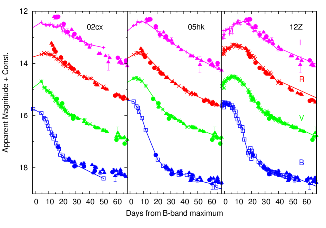
Figure 14: The best-fit LCs of SN 2014dt in the $BVRI$-band. These were derived in order to construct ‘combined’ LCs in the period before the discovery (i.e., around the maximum of SN 2014dt). We adopt the LCs of SNe 2002cx (left panel), 2005hk (middle) and 2012Z (right) as templates (see Appendix for details). For SN 2014dt, the symbols are plotted in the same manner as in Figure 3. We show the fitted reference LCs by crosses connected by solid lines.

References

- [1] Akitaya, H., et al. 2014, Proc. SPIE, 9147, 91474O
- [2] Anupama, G. C., Sahu, D. K., & Jose, J., 2005, A&A, 429, 667
- [3] Arnett, W. D., 1982, ApJ, 253, 785
- [4] Barna et al. 2017, MNRAS, 471, 4865
- [5] Bertin, E., Arnouts, S., 1996, A&AS, 117, 393
- [6] Blondin, S., et. al. 2012, AJ, 143, 126
- [7] Bose, S., & Kumar, B., 2014, ApJ, 782, 98
- [8] Branch, D., Baron, E., Thomas, R. C., Kasen, D., Li, W., & Filippenko, A. V., 2004, PASP, 116, 903
- [9] Brown, P. J., Breeveld, A. A., Holland, S., Kuin, P., Pritchard, T., 2014, Ap&SS, 354, 89
- [10] Dessart, L., & Hillier, D. J., 2005, A&A, 439, 671
- [11] Cardelli, J. A., Claython, G. C., & Mathies, J. S., 1989, ApJ, 345, 245
- [()] Chornock, R., Filippenko, A. V., Branch, D., Foley, R. J., Jha, S., & Li, W., 2006, PASP, 118, 722
- [()] Childress, M. J., et al. 2015, MNRAS, 454, 3816
- [12] van Dokkum, P. G., 2001, PASP, 113, 1420
- [13] van Dokkum, P. G., Bloom, J., Tewes, M., 2012, ASCL, 07005
- [14] Fink, M., et. al. 2014, MNRAS, 438, 1762
- [()] Foley, R. J., et al. 2009, AJ, 138, 376
- [()] Foley, R. J., et al. 2010, AJ, 140, 1321
- [15] Foley, R. J., et al. 2013, ApJ, 767, 57
- [16] Foley, R. J., McCully, C., Jha, S. W., Bildsten, L., Fong, W., Narayan, G., Rest, A., & Stritzinger, M. D., 2014, ApJ, 792, 29
- [17] Foley, R. J., Van Dyk, S. D., Jha, S. W., Clubb, K. I., Filippenko, A. V., Mauerhan, J. C., Miller, A. A., & Smith, N., 2015, ApJ, 798, 37
- [18] Foley, R. J., Jha, S. W., Pan, Y., Zheng, W., Bildsten, L., Filippenko, A. V., & Kasen, D., 2016, MNRAS, 461, 433
- [19] Fox, O., et al. 2016, ApJ, 816, 13
- [20] Friedman, A. S., 2015, ApJS, 220, 9
- [21] Fukugita, M., Shimasaku, K., & Ichikawa, T., 1995, PASP, 107, 945
- [22] Ganeshalingam, M., et al. 2010, ApJS, 190, 418
- [23] Graham, M. L., et. al. 2015, MNRAS, 446, 2073
- [24] Guillochon, J., Parrent, J., Kelley, L. Z., Margutti, R., 2017, ApJ, 835, 64
- [()] Hicken, M., et al. 2009, ApJ, 700, 331
- [()] Hicken, M., et al. 2012, ApJS, 200, 12
- [()] Höeflich, P., Khokhlov, A. M., & Wheeler, J. C., 1995, ApJ, 444, 831
- [()] Höeflich, P., & Khokhlov, A. M., 1996, ApJ, 457, 500
- [25] Jha, S., Branch, D., Chornock, R., Foley, R. J., Li, W., Swift, B. J., Casebeer, D., & Filippenko, A. V., 2006, AJ, 132, 189
- [()] Jha, S., Riess, A. G., & Kirshner, R. P., 2007, ApJ, 659, 122
- [26] Kashikawa, N., et al. 2002, PASJ, 54, 819
- [27] Kawabata, K. S., et al. 2008, Proc. SPIE, 7014, 70144
- [28] Kawabata, K. S., et. al. 2014, ApJ, 795, L4
- [29] Kromer, M., et. al. 2013, MNRAS, 429, 2287
- [30] Kromer, M., et. al. 2015, MNRAS, 450, 3045
- [31] Krisciunas, K., et al. 2003, AJ, 125, 166
- [32] Krisciunas, K., et al. 2017, AJ, 154, 211
- [33] Landolt, A. U., 1992, AJ, 104, 340
- [34] Leloudas, G, et al. 2009, A&A, 505, 265
- [35] Li H., & McCray, R., 1993, ApJ, 405, 730
- [36] Li, W., et al. 2003, PASP, 115, 453
- [37] Maeda, K., Mazzali, P. A., Deng, J., Nomoto, K., Yoshii, Y., Tomita, H., & Kobayashi, Y., 2003, ApJ, 593, 931
- [38] Maeda, K., et. al. 2010, Nature, 466, 82
- [39] Magee, et. al. 2016, A&A, 589, 89
- [40] Magee, et. al. 2017, A&A, 601, 62
- [41] Maguire, K., et. al. 2010, MNRAS, 404, 981
- [42] McClelland, C. M., et al. 2010, ApJ, 720, 704
- [43] McCully, C., et. al. 2014, Nature, 512, 54
- [44] McCully, C., et. al. 2014, ApJ, 786, 134
- [45] Moriya, T., Tominaga, N., Tanaka, M., Nomoto, K., Sauer, D. N., Mazzali, P. A., Maeda, K., & Suzuki, T., 2010, ApJ, 719, 1445
- [46] Nagao, T., Maeda, K., Yamanaka, M., 2017, ApJ, 835, 143
- [47] Nakano, S., et al. 2014, CBET, 4011, 1
- [48] Narayan, G., Foley, R. J., Berger, E., et al. 2011, ApJ, 731, 11
- [49] Nomoto, K., Sugimoto, N., Neo, S., 1976, Ap&SS, 39, L37
- [50] Ochner, P., Tomasella, L., Benetti, S., Cappellaro, E., Elias-Rosa, N., Pastorello, A., & Turatto, M., 2014, CBET, 4011, 2
- [51] Pastorello, A., et. al. 2007, MNRAS, 377, 1531
- [52] Parrent, J. T., et al. 2012, ApJ, 752, 26
- [53] Pereira, R., et al. 2013, A&A, 554, A27
- [54] Perlmutter, S., et. al. 1999, ApJ, 517, 565
- [55] Phillips, M. M., 1993, ApJ, 413, 105
- [56] Phillips, M. M., et al. 2007, PASP, 119, 360
- [57] Pignata, G., et al. 2008, MNRAS, 388, 971
- [58] Pignata, G., et. al. 2004, MNRAS, 355, 178
- [59] Richmond, M. W., & Smith, H, H. A., 2012, JAVSO, 40, 872
- [60] Richardson, D., Thomas, R. C., Casebeer, D., Blankenship, Z., Ratowt, S., Baron, E., & Branch, D., 2001, AAS, 199, 8408
- [61] Roy, R., et al. 2011, ApJ, 736, 76
- [62] Sahu, D., et al. 2008, ApJ, 680, 580
- [63] Sandage, A., Saha, A., Tammann, G. A., Labhardt, L., Panagia, N., & Macchetto, F. D., 1996, ApJ, 460, L15
- [64] Schlegel, D. J., Finkbeiner, D. P., & Davis, M., 1998, ApJ, 500, 525
- [65] Schoeniger, F., & Sofue, Y., 1997, A&A, 323, 14
- [66] Silverman, J. M., et al. 2012, MNRAS, 425, 1789
- [67] Singh, M., et al. 2018, MNRAS, 474, 2551
- [68] Skrutskie et al. 2006, AJ, 131, 1163
- [69] Smith, J. A., et. al. 2002, AJ, 123, 2121
- [70] Stritzinger, M., et al. 2002, AJ, 124, 2100
- [71] Stritzinger, M., & Leibundgut, B., 2005, A&A, 431, 423
- [72] Stritzinger, M., & Sollerman, J., 2007, A&A, 470, L1
- [73] Stritzinger, M. D., et al. 2014, A&A, 561, A146
- [74] Stritzinger, M. D., et al. 2015, A&A, 573, A2
- [75] Suntzeff, N. B., et al. 1999, AJ, 117, 1175
- [76] Szalai, T., Vinkó, J., Sárneczky, K., et al. 2015, MNRAS, 453, 2103
- [77] Thomas, R. C., Nugent, P. E., Meza, J. C., 2011, PASP, 123, 237
- [78] Tomasella, L., Cappellaro, E., Benetti, S., et al. 2016, MNRAS, 459, 1018
- [79] Tomita, H., et. al. 2006, ApJ, 664, 400
- [80] Valenti, S., et. al. 2009, Nature, 459, 674
- [81] Wang, X., et. al. 2009, ApJ, 697, 380
- [82] Yamanaka, M., et al. 2015, ApJ, 806, 191
- [83] Yamanaka, M., et al. 2016, PASJ, 68, 68
- [84] Yaron, O., & Gal-Yam, A., 2012, PASP, 124, 668
- [85] Zhang, J., Wang, X., Bai, J., Zhang, T., Wang, B., Liu, Z., Zhao, X., & Chen, J., 2014, AJ, 148, 1
- [86] Zhang, K., et al. 2016, ApJ, 820, 67