RNA polymerase interactions and elongation rate

Abstract

We show that non-steric molecular interactions between RNA polymerase (RNAP) motors that move simultaneously on the same DNA track determine strongly the kinetics of transcription elongation. With a focus on the role of collisions and cooperation, we introduce a stochastic model that allows for the exact analytical computation of the stationary properties of transcription elongation as a function of RNAP density, their interaction strength, nucleoside triphosphate concentration, and rate of pyrophosphate release. Cooperative pushing, i.e., an enhancement of the average RNAP velocity and elongation rate, arises due to stochastic pushing. This cooperative effect cannot be explained by steric hindrance alone but requires a sufficiently strong molecular repulsion. It disappears beyond a critical RNAP density, above which jamming due to collisions takes over. For strong stochastic blocking the cooperative pushing is suppressed at low RNAP densities, but a reappears at higher densities.

${}^{~{}1}$Instituto de Matemática e Estátistica, Universidade de São Paulo, Rua do Matão, 1010, CEP 05508-090, São Paulo - SP, Brazil
Email: belitsky@ime.usp.br

${}^{~{}2}$Institute of Complex Systems II, Theoretical Soft Matter and Biophysics, Forschungszentrum Jülich, 52425 Jülich, Germany
Email: g.schuetz@fz-juelich.de

1 Introduction

RNA polymerase (RNAP) is a molecular motor that transcribes the information coded in the base pair sequence of DNA into an RNA. The process is initiated at a promoter sequence on the DNA. Stepping along the base pairs of the DNA, the RNAP forms the transcription elongation complex (TEC) which polymerizes the monomeric subunits of the RNA by the addition of nucleotides, as determined by the corresponding sequence on the template DNA [1, 2]. To this end, the RNAP locally creates the so-called transcription bubble by unzipping the two DNA strands as it progresses. The elongation process ends when the TEC reaches the termination sequence. Then the nascent RNA is released by the RNAP and serves as a template for translation into proteins (in the case of messenger RNA) or facilitates the formation of RNA-protein complexes such as ribosomes. Thus RNAPs play a central role in gene expression and also as therapeutic drug targets [3].

Here we focus on the kinetics of the elongation stage where each successful addition of ribonucleotides to the growing RNA transcript is accompanied by a biased random walk of the RNAP along the DNA with a step length of one base pair for each translocation [4, 5]. Our main interest is the impact of interactions between RNAP on the average speed of an individual RNAP which determines the overall rate of elongation.

The intrinsically stochastic dynamics of a single RNAP has been studied in great detail. The major and generic features of the multi-step mechano-chemical pathway of individual RNAP motors during each elongation step are: (1) Nucleoside triphosphate (NTP) binding at a catalytic site within the transcription bubble, (2) NTP hydrolysis, (3) Release of pyrophosphate (PP_i, one of the products of hydrolysis), (4) Forward step of the RNAP along the DNA template by one base pair (bp) [2, 6]. Recently, the mechanism of NTP binding to the active site [7] and PP_i release [8] were studied with atomistic simulations in great detail for T7 RNA Polymerase. Also recently, the role of trigger loop folding-unfolding on the RNAP translocation was elucidated for the RNAP of Escherichia coli [9]. For a recent more detailed description, see [10].

If more than one RNAP molecule initiates from the same promoter one cannot ignore their mutual interactions. On the one hand, pausing RNAP may block the advancement of trailing RNAP and thus induce “traffic jams” [11, 12] and phase transitions in the rate of elongation [13]. On the other hand, by the same token the interaction has been demonstrated to be cooperative: Trailing RNAP strongly prevent backtracking, and even “push” the leading RNAP out of pause sites [14, 15, 16, 17, 18, 19, 20]. Thus one is faced with the apparently paradoxical picture that the appearance of traffic jam would suggest a reduction of the average rate of elongation, while cooperative behaviour indicates an enhancement.

How RNAP interactions affect the rate of elongation is not known quantitatively nor is their precise nature. Most modelling approaches to molecular motor traffic that are based on generalizations of the asymmetric simple exclusion process (ASEP), a generic Markovian lattice gas model, assume only a hard core repulsion corresponding to pure steric hindrance on contact. This approach successfully captures the traffic jam phenomenon and other kinetic properties of the transcription process [21]. However, this interaction does not explain pushing as the rate of forward steps along the DNA in such models does not depend on the presence of motors in the backward direction.

This shortcoming is addressed in a number of recent works. Galburt et al. [19] employed transition rate theory to determine rates of translocation by postulating a phenomenological free-energy landscape for two neighbouring RNAP interacting via a hard-core potential. They concluded that pushing occurs only in cases where the transition state of the active particle is relatively early during a step. Costa et al. [22] introduced a model that generalizes the stochastic sequence-dependent model of Bai et al. [23, 24] such that collisions between elongating RNAP modify their elongation rates. For the sequences that were investigated by numerical simulation an acceleration of transcription up to 48% was observed when collisions are allowed. Teimouri et al [25] consider a generic Markovian model for molecular motors where the pushing and collisions are explicitly put into the model by rates that are different from the single-motor step rate when a motor attempts to move close to a paused motors or when it moves away from it. With numerical simulation and analytical mean field approximation it is shown that there is an optimal repulsive interaction strength that leads to a maximal particle flux, which in the context of our discussion translates into an optimal elongation rate. In this model the mechano-chemical cycle that RNAP undergo during translocation is ignored. Heberling et al. [26] argue that the torque produced by RNAP motion on helically twisted DNA leads to fewer collisions and thus explains transcription enhancement. This hypothesis is supported by Monte-Carlo simulation of a generalized ASEP in which the rate of translocation depends on the torque between the polymerase and its closest two neighboring polymerases. The amount of torque is, in turn, the result of the relative motion of RNAPs on the DNA strand. However, the notion of transcription enhancement due to a reduced number of collisions is at odds with the pushing picture which relies on collisions of the trailing RNAP with a pausing RNAP.

Here we take a different approach. We propose a stationary distribution of the chemical states and the relative distances between RNAPs along the template DNA. From this distribution we determine Markovian stochastic transition mechanisms that on the one hand are compatible with stationarity and on the other hand take into account the main processes in the mechano-chemical RNAP stepping cycle as well as not only steric hard-core repulsion, but also a short-range term that captures the interaction when two RNAP are very close to each other. This approach enables us to make exact analytical computations for collective stationary quantities rather than having to rely on numerical simulation or analytical mean-field theory which do not allow for any rigorous estimate of the approximation error.

It will transpire that hard-core repulsion alone does not allow to capture any pushing phenomenon. However, the presence of an additional short-range repulsion turns out to lead to stochastic pushing (which is not an input into our model) and thus explains it as a general consequence of short-range repulsion between neighbouring RNAP moving stochastically along the DNA track. The effect of the stochastic pushing on the collective average motor velocity and hence on the average elongation rate depends on the average density of interacting RNAP along the DNA. At sufficiently low densities the cooperative effect of pushing prevails over blocking and leads to an enhanced RNAP speed, compared to the average speed of an isolated single motor. Beyond a critical density, however, the average velocity starts to decrease, even though the average elongation rates generated by the collective action of all RNAP still increases with density. At a second higher critical density blocking prevails and also the average elongation rate decreases with further increasing density. Thus our approach accounts both for cooperative pushing and jamming. Interestingly, for sufficiently strong repulsion the average elongation rate can exhibit two maxima at different RNAP densities. Moreover, the model makes analytical predictions about how the motor velocity and elongation rate change when the concentration of NTP and the rate of PP_i release vary.

In the next section we formulate the mathematical model and review some of the theoretical and empirical background that motivates it. In the third section we present and discuss our results. First we focus on minimal-range interaction and present exact analytic expressions for the RNAP average velocity and transcription rate as functions of the RNAP density and interaction strength. Then we extend the discussion to an extended interaction range of the microscopic processes without impact on the stationary distribution. In the concluding section we summarize the gist of our approach and the main findings. The mathematical derivations of the results are presented in an Appendix.

2 Methods

We address the questions detailed in the introduction with a stochastic model for interacting RNAP that we introduce here. The model is a Markov process whose exact stationary properties, in particular, the average rate of transcription elongation, can be computed analytically as function of the model parameters. First we describe the model for the stochastic dynamics of an isolated RNAP, following [6]. In a second step we introduce interactions.

2.1 Single-RNAP dynamics

As mentioned above, the RNAP undergoes various transformations during each elongation step, see [10] for a recent discussion. Here we do not aspire a detailed description. In the reduced description of Wang et al [6], which accounts rather well for various experimentally established features of the kinetics of single RNAP, and which is adequate as a starting point for the purposes of this work, the rate-limiting step is the PP_i release from the catalytic site [28]. An RNAP carrying an RNA transcript of length $n$ thus appears in only two distinct polymerization states, namely with or without PP_i bound to it. It moves forward along the DNA only after PP_i release by one bp, corresponding to a step length $\delta=0.34nm$.

It is natural to describe the state of an RNAP mathematically not in terms of the length $n$ of the RNA transcript attached to it, but to consider $n$ to mark the corresponding base pair on the template DNA. We denote the RNAP state without PP_i by 1 and when it is bound by 2. Thus the translocation of the RNAP from base pair $n$ to $n+1$ corresponds to a directed random step on a one-dimensional lattice from site $n$ to $n+1$ provided the RNAP is in state 1. We denote the rate at which this step occurs by $\omega^{\star}$. The processes that lead to translocation are fast by comparison to the PP_i release and thus conflate into the translocation step itself, which means that the RNAP arrives at site $n+1$ in state 2 with PP_i bound. It can move again only after PP_i is released, which happens with a rate that we denote by $\kappa^{\star}$. This reduced minimal reaction scheme is sketched in Figure 1.

Figure 1: Minimal reaction scheme of RNAP translocation. The RNAP can move from base pair $n$ to $n+1$ provided it is in state $1_{n}$ (no pyrophospate bound to it) with an effective rate $\omega^{\star}$ through a series of processes involving NTP binding to the active site and NTP hydrolysis which results in a PP_i bound state in the transcription elongation complex (state $2_{n+1}$). Only after PP_i release with rate $\kappa^{\star}$ (transition from state $2_{n+1}$ to state $1_{n+1}$) the RNAP can perform the next translocation step. Reverse reactions (not considered here) are indicated with thin dashed arrows.

The reverse processes are possible, but occur with smaller rates [6] that we neglect. For the purpose of elucidating the role of interactions we also ignore the sequence dependence and the role of the trigger loop in the translocation mechanism. Following [6] we assume that the PP_i release rate $\kappa^{\star}$ is independent of the NTP concentration while the translocation rate $\omega^{\star}$ is proportional to it. In the setting considered by Wang et al. one has under load-free conditions

$$\kappa^{\star}=31.4s^{-1},\quad\omega^{\star}=[NTP](\mu M)^{-1}s^{-1}$$ (2.1)

where $[NTP]$ is the NTP concentration. The rates $\kappa^{\star}$ and $\omega^{\star}$ are of similar magnitude for $[NTP]$ around $30\mu M$. The translocation rate $\omega^{\star}$ is a free parameter of our model. Under cellular conditions, RNAP transription leads to downstream supercoiling that generates a load force of $6pN$ [27]. We ignore this effect as it only renormalizes the translocation rate by a factor of approximately $\exp{(-6pN\cdot 0.34nm)/k_{B}T}\approx 0.6$.

2.2 RNAP interactions

We extend the two-state random walk model for single RNAP to a Markov process of interacting random walks. The typical size of a transcription bubble is around 15 bp [6, 29] whereas the TEC covers a DNA segment of up to 35 bp. We simplify the complicated geometry of the TEC by representing it as a rod covering $\ell$ lattice sites, where $\ell$ is parameter of our model that can be adjusted as needed. We number the RNAPs sequentially from 1 to $N$ and denote by $x_{i}$ the (integer) lattice position of the left end of the $i^{th}$ rod in the random walk model, which corresponds to the trailing side of the corresponding TEC. Then $x_{i}+\ell-1$ is the lattice position of the “front” side of the TEC. We say that two rods (TECs) $i$ and $i+1$ are neighbours when the front of rod $i$ and the left edge of rod $i+1$ occupy neighbouring lattice sites, i.e., when $x_{i+1}=x_{i}+\ell$. For technical reasons and since we are interested only in the elongation stage of transcription we take a lattice of $L$ sites with periodic boundary conditions.

2.2.1 Short-range contribution to hard-core repulsion

Both for RNAP and other molecular motors the modelling of steric hindrance by a hard-core repulsion alone has a very long history, starting with the pioneering work of MacDonald et al [30] on ribosomes, see e.g. [12, 31, 32, 33, 34, 35, 36, 37, 38] for later developments concerning ribosomes, RNAP and other molecular motors. In the framework of our model this means that translocation cannot occur if the site $x_{i}+\ell$ next to the tip of the RNAP $i$ is occupied by a leading RNAP $i+1$. Thus traffic jams of molecular motors may form [38]. However, as shown below, this approach does not allow for pushing.

Indeed, recent data suggest that the description of the free energy landscape of two neighbouring TECs by just a hard-core interaction is inappropriate when the leading polymerase is unable to move forward due to nucleotide starvation. Under these conditions, the system exhibits elastic deformations [16, 19]. In order to capture this effect we introduce an interaction that has short-ranged contributions to hard-core repulsion. Since we do not wish to use pushing as an input into model but derive it analytically, we define processes along the lines indicated above for a single RNAP, but with rates that depend on the presence of nearby RNAP. These rates are given initially as free parameters. Then we fix mathematically rigorously relations between the proposed transition rates to ensure stationarity of the distribution. This will indicate whether the rates are in a range compatible with pushing or not.

2.2.2 Stationary distribution

Hardcore repulsion means that configurations such that $x_{i+1}=x_{i}+\ell-1$ are forbidden since in such a case the front of rod $i$ and the end of rod $i+1$ would occupy the same site. Correspondingly, the stationary distribution gives give probability 0 to such configurations. Moreover, since TECs cannot overtake each other, the coordinates $x_{i}$ will stay ordered at all times, i.e., only RNAP configurations satisfying the ordering condition $x_{i+1}\geq x_{i}+\ell$ have non-zero probability. We shall refer to such configurations as allowed configurations. An allowed configuration of $N$ RNAPs, which we denote by $\boldsymbol{\eta}$, is thus specified by a coordinate vector $\mathbf{x}=(x_{1},\dots,x_{N})$ with ordered integer coordinates and a state vector $\mathbf{s}=(s_{1},\dots,s_{N})$ with state variables $s_{i}\in\{1,2\}$.

For the stationary distribution of the interacting RNAPs we assume for the interaction part of $N$ RNAPs at positions $\mathbf{x}=(x_{1},\dots,x_{N})$ in addition to hardcore repulsion an effective short range interaction energy of the form

$$U(\mathbf{x})=J\sum_{i=1}^{N}\delta^{L}_{x_{i+1},x_{i}+\ell}.$$ (2.2)

Here $\delta^{L}$ denotes the Kronecker symbol with arguments understood modulo $L$ due to periodic boundary conditions. Positive $J$ corresponds to repulsion.

We denote by $N^{\alpha}$ the fluctuating number of RNAPs in state $\alpha\in\{1,2\}$, so that $N=N^{1}+N^{2}$. We also define the excess $B(\mathbf{s})=N^{1}-N^{2}$. The stationary distribution for allowed configurations thus takes the form

$$\pi^{\ast}(\boldsymbol{\eta})=\frac{1}{Z}\pi(\boldsymbol{\eta})$$ (2.3)

with the Boltzmann weights

$$\pi(\boldsymbol{\eta})=\exp{\left[-\frac{1}{k_{B}T}\left(U+\lambda B\right)\right]}$$ (2.4)

and the partition function

$$Z=\sum_{\boldsymbol{\eta}}\pi(\boldsymbol{\eta}).$$ (2.5)

The chemical potential $\lambda$ is a Lagrange multiplier that takes care of the fluctuations in the excess

$$B(\mathbf{s})=\sum_{i=1}^{N}(3-2s_{i})$$ (2.6)

due to the interplay of NTP hydrolysis and PP_i release.

For later use we introduce the parameters

$$x=\mathrm{e}^{\frac{2\lambda}{k_{B}T}},\quad y=\mathrm{e}^{\frac{J}{k_{B}T}}$$ (2.7)

to work with, instead of $\lambda$ and $J$. Positive $\lambda$ (i.e., $x>1$) corresponds to an excess of RNAP in state 1. Repulsive interaction corresponds to $y>1$.

2.2.3 Kinetic assumptions

The rate-limiting processes that occur during transcription elongation must be consistent with the stationarity of the distribution (2.3). For the the kinetics of a single RNAP model we adopt the results of [6] for the temperature and concentration dependence of the translocation rate $\omega^{\star}$ appearing in (2.1) as well as a constant value for $\kappa^{\star}$. However, as mentioned above, in the interacting case we allow these rates to depend parametrically on the presence of neighbouring RNAP. We consider separately two different forms of a kinetic short-range interaction which influence the rates of translocation and PP_i release.

A) Minimal kinetic interaction range

The rate for a move by one step of rod $i$ covering sites from $x_{i}$ to $x_{i}+\ell-1$ depends on the occupation of the directly neighboring sites $x_{i-1}$ and $x_{i+\ell}$. As in the single-RNAP case the rod needs to be in state 1 to move and arrives at the target site in state 2.

From the hard-core repulsion we require that an RNAP can move forward by one site, if demanded by its own mechanochemistry, provided the target site $x_{i+\ell}$ is not already covered. Thus the configuration-dependent translocation rate for rod $i$ from position $x_{i}$ to position $x_{i}+1$ is of the form

$$\omega_{i}(\boldsymbol{\eta})=\omega^{\star}\delta_{s_{i},1}\left(1+d^{1\star}\delta_{x_{i-1}+\ell,x_{i}}\right)\left(1-\delta_{x_{i}+\ell,x_{i+1}}\right)$$ (2.8)

with “bare” rate $\omega^{\star}$ when both neighbouring sites $x_{i}-1$ and $x_{i+\ell}$ are empty and a correction given by the phenomenological dimensionless interaction parameter $d^{1\star}\geq-1$ (to ensure positivity of the rate) when rods $i-1$ and $i$ are neighbours. The overall factor $\left(1-\delta_{x_{i+\ell},x_{i+1}}\right)$ is zero when rods $i$ and $i+1$ are neighbours and thus expresses hard-core repulsion.

Likewise, we parametrize the rate for PP_i release as

$$\kappa_{i}(\boldsymbol{\eta})=\kappa^{\star}\delta_{s_{i},2}\left(1+f^{1\star}\delta_{x_{i-1}+\ell,x_{i}}+f^{\star 1}\delta_{x_{i}+\ell,x_{i+1}}+f^{1\star 1}\delta_{x_{i-1}+\ell,x_{i}}\delta_{x_{i}+\ell,x_{i+1}}\right)$$ (2.9)

with the bare release rate $\kappa^{\star}$ and interaction terms coming from the potential presence of neighbouring rods.

The master equation for the probability $P(\boldsymbol{\eta},t)$ of finding the rods at time $t$ in a configuration $\boldsymbol{\eta}$ thus reads

$$\frac{\mathrm{d}}{\mathrm{d}t}P(\boldsymbol{\eta},t)=\sum_{i=1}^{N}\left[\omega_{i}(\boldsymbol{\eta}_{tl}^{i})P(\boldsymbol{\eta}_{tl}^{i},t)+\kappa_{i}(\boldsymbol{\eta}_{rel}^{i})P(\boldsymbol{\eta}_{rel}^{i},t)-(\omega_{i}(\boldsymbol{\eta})+\kappa_{i}(\boldsymbol{\eta}))P(\boldsymbol{\eta},t)\right]$$ (2.10)

where $\boldsymbol{\eta}_{tl}^{i}$ is the configuration that leads to $\boldsymbol{\eta}$ before a translocation of RNAP $i$ (i.e., with coordinate $x^{tl}_{i}=x_{i}-1$ and state $s^{tl}_{i}=3-s_{i}$) and $\boldsymbol{\eta}_{rel}^{i}$ is the configuration $\boldsymbol{\eta}$ before PP_i release at RNAP $i$ (i.e., with coordinate $x^{rel}_{i}=x_{i}$ and state $s^{rel}_{i}=3-s_{i}$. Due to periodicity, the positions $x_{i}$ of the rods are counted modulo $L$ and labels $i$ are counted modulo $N$.

B) Extended kinetic interaction range

As we will see, the form (2.3) of the stationary distribution does not uniquely fix the rates for translocation and PP_i release. In particular, one may explore a dependence of these rates over distances of neighbouring rods of more than one site.

For the configuration-dependent translocation rate for rod $i$ we assume a dependence on whether the configuration after the jump leads to a new neighbouring pair of rods or not, as this changes the effective energy (2.2) and hence the Boltzmann weight (2.4) of the configuration in the distribution (2.3). This yields

$$\omega_{i}(\boldsymbol{\eta}) = \omega^{\star}\delta_{s_{i},1}\left(1+d^{1\star}\delta_{x_{i-1}+\ell,x_{i}}+d^{\star 1}\delta_{x_{i+1},x_{i}+\ell+1}\right)\left(1-\delta_{x_{i+1},x_{i}+\ell}\right)$$ (2.11)

with a further dimensionless interaction parameter $d^{\star 1}$.

For the rate of PP_i release, which does no lead to any change in the effective energy (2.2), we allow for a dependence on the presence neighboring RNAP of the form

$$\kappa_{i}(\boldsymbol{\eta}) = \kappa^{\star}\delta_{s_{i},2}\left[1+f^{1\star}\delta_{x_{i-1}+\ell,x_{i}}+f^{\star 1}\delta_{x_{i}+\ell,x_{i+1}}+f^{1\star 1}\delta_{x_{i-1}+\ell,x_{i}}\delta_{x_{i}+\ell,x_{i+1}}\right.$$ (2.12)

$$\left.+f^{10\star}(1-\delta_{x_{i-1}+\ell,x_{i}})\delta_{x_{i-1}+\ell+1,x_{i}}+f^{\star 01}(1-\delta_{x_{i}+\ell,x_{i+1}})\delta_{x_{i+1},x_{i}+\ell+1}\right].$$

The master equation for the extended process is of the same form as the master equation (2.10) since the allowed transitions are the same, the only difference being their rate. We do not specify the interactions that lead to the parameters appearing in the rates (2.8),(2.9), (2.11), and (2.12) since we do not have sufficient experimental knowledge of the underlying processes on molecular level. We stress that one cannot impose detailed balance since the system is not in thermal equilibrium. We can just state that for a stationary distribution the left hand side of the many-particle master equation (2.10) is equal to 0, by definition of stationarity. Thus the condition of stationary of the proposed distribution (2.3) determines the parameters that enter the interaction the parameters appearing in the rates (2.8),(2.9), (2.11), and (2.12).

3 Results and Discussion

Due to the stochastic dynamics all quantities of interest are fluctuating. However, under high growth conditions a large number of RNAP transcribe simultaneously and fluctuations get washed out. Hence in this work our main concern are stationary averages. These are not averages over different cells where various external factors may lead to variations, but averages over the fluctuations inherent to RNAP transcription from the same DNA template. We denote the average density of RNAP by $\rho$ by which we mean the average number of RNAP on a DNA sequence of $L$ bp. We also recall the definitions (2.7) that will be used extensively.

3.1 Stationarity condition

As pointed out above, given the stationary distribution (2.3), the transition rates $\omega_{i}(\boldsymbol{\eta})$ and $\kappa_{i}(\boldsymbol{\eta})$ cannot be chosen freely. We stress that, in fact, it is not even a priori clear whether a process exists for which the distribution (2.3) is stationary and which has rates of the form (2.8) and (2.9) or (2.11) and (2.12). It is therefore rather non-trivial that, as shown in the Appendix, the requirement of stationarity of the probability distribution (2.3) fixes in a non-trivial fashion the parameters $x,y$ (2.7) and the rates (2.11) and (2.12), up to four free parameters $\kappa^{\star},\omega^{\star},d^{1\star},d^{\star 1}$. In terms of these parameters one obtains the relations

$$x=\frac{\omega^{\star}}{\kappa^{\star}}$$ (3.1)

$$y=\frac{1+d^{1\star}}{1+d^{\star 1}}$$ (3.2)

$$f^{1\star}=d^{1\star}\frac{x}{1+x}-\frac{1}{1+x}$$ (3.3)

$$f^{\star 1}=d^{1\star}\frac{1}{1+x}-\frac{x}{1+x}$$ (3.4)

$$f^{1\star 1}=-d^{1\star}$$ (3.5)

$$f^{10\star}=d^{\star 1}\frac{1}{1+x}$$ (3.6)

$$f^{\star 01}=d^{\star 1}\frac{x}{1+x}$$ (3.7)

which must be satisfied for (2.3) to be stationary. The relations for minimal interaction range follow by setting $f^{\star 01}=f^{10\star}=d^{\star 1}=0$. Here we only outline the strategy of the proof. More mathematical details are given in the appendix.

Dividing (2.10) by the stationary distribution (2.3), the stationarity condition becomes

$$\sum_{i=1}^{N}\left[\omega_{i}(\boldsymbol{\eta}_{tl}^{i})\frac{\pi(\boldsymbol{\eta}_{tl}^{i})}{\pi(\boldsymbol{\eta})}+\kappa_{i}(\boldsymbol{\eta}_{rel}^{i})\frac{\pi(\boldsymbol{\eta}_{rel}^{i})}{\pi(\boldsymbol{\eta})}-(\omega_{i}(\boldsymbol{\eta})+\kappa_{i}(\boldsymbol{\eta}))\right]=0.$$ (3.8)

Now we introduce the quantities

$$D_{i}(\boldsymbol{\eta}) = \omega_{i}(\boldsymbol{\eta}_{tl}^{i})\frac{\pi(\boldsymbol{\eta}_{tl}^{i})}{\pi(\boldsymbol{\eta})}-\omega_{i}(\boldsymbol{\eta})$$ (3.9)

$$F_{i}(\boldsymbol{\eta}) = \kappa_{i}(\boldsymbol{\eta}_{rel}^{i})\frac{\pi(\boldsymbol{\eta}_{rel}^{i})}{\pi(\boldsymbol{\eta})}-\kappa_{i}(\boldsymbol{\eta}).$$ (3.10)

Taking into account periodicity, the stationarity condition (3.8) is satisfied if the lattice divergence condition

$$D_{i}(\boldsymbol{\eta})+F_{i}(\boldsymbol{\eta})=\Phi_{i}(\boldsymbol{\eta})-\Phi_{i+1}(\boldsymbol{\eta})$$ (3.11)

holds for all allowed configurations with a family of functions $\Phi_{i}(\boldsymbol{\eta})$ satisfying $\Phi_{N+1}(\boldsymbol{\eta})=\Phi_{1}(\boldsymbol{\eta})$. The lattice divergence condition can be understood as a specific discrete form of Noethers theorem.

A further ingredient is to consider the headway, i.e., the number of empty sites $m_{i}$ between neighbouring rods $i$ and $i+1$, as random variable rather than the actual positions $x_{i}$, which is possible due to translation invariance. A configuration of RNAPs is then specified by the distance vector $\mathbf{m}:=(m_{1},\dots,m_{N})$ and the state vector $\mathbf{s}$. The energy (2.2) becomes $E(\mathbf{m})=J\sum_{i}\delta_{m_{i},0}$. As a result, the stationary distribution (2.3) becomes a product measure in the new distance variables $m_{i}$. The rates $\omega_{i}$ and $\kappa_{i}$ are functions of the distances $m_{i-1}$ and $m_{i}$. By somewhat lengthy, but straightforward computations one then finds that the lattice divergence condition is satisfied if and only if relations (3.1) - (3.7) are satisfied.

3.2 Pure hard-core repulsion

It is interesting to note that In the absence of a static nearest-neighbour interaction ($J=0$) other than hard-core repulsion one has $y=1$. Then the stationarity conditions (3.1) - (3.7) force all parameters that determine the interaction contributions to the translocation rate and to the PP_i release rate to be zero. Thus a pure hard-core repulsion is compatible with transition rates of the interacting system that are identical to the transition rates of a single RNAP. Therefore, stationary of a distribution corresponding to hard-core repulsion only is not compatible with any kinetic mechanism that produces the experimentally observed pushing phenomenon.

3.3 Pushing and blocking

As stressed above, the model assumptions include the form of the stationary distribution (2.3) and some assumptions on the form of the transition rates, as expressed by the parameters appearing in (2.8) and (2.9) for minimal kinematic interaction range and (2.11) and (2.12) resp. for the extended kinematic interaction range. There is no assumption on the magnitude of these parameters. The quantitative relations (3.1) - (3.7) are consequences arising from requiring stationarity of the distribution (2.3).

We consider first the choice of minimal kinematic interaction range. Inserting (3.2) with $d^{\star 1}=0$ into the translocation rate (2.8) one finds the translocation rate

$$\omega_{i}(\boldsymbol{\eta})=\omega^{\star}\delta_{s_{i},1}y^{\delta_{x_{i-1}+\ell,x_{i}}}\left(1-\delta_{x_{i}+\ell,x_{i+1}}\right).$$ (3.12)

This form of the rate means the following. If RNAP $i$ has no left trailing neighbour and the neighbouring site in forward direction is free, then translocation takes place with the rate $\omega^{\star}$ of an isolated RNAP. However, if a trailing RNAP has arrived to the left of the RNAP, then translocation takes place with rate

$$\omega^{push}=y\omega^{\star}.$$ (3.13)

For repulsive static interaction ($J>0$) one has $y>1$. Thus the trailing RNAP pushes the leading RNAP, as observed in experiments [14, 15]. Blocking, i.e., the prevention of a forward step through the presence of an RNAP on the target site, occurs in the same manner as in the case of pure hard-core repulsion, since the translocation rate in the minimal interaction range scheme is not sensitive to the occupation of the location 2 sites ahead of its present position. The pushing which is discussed here in terms of the rate $\omega^{push}$ will from now on be referred to as stochastic pushing, as opposed to a collective increase of the average RNAP velocity discussed below.

We regard to the extended interaction range we point out that according to (3.2), repulsion corresponds to $d^{1\star}>d^{\star 1}$. The significance of this relation becomes clear by noting that according to the definition (2.11) the quantity $\omega^{\star}(1+d^{1\star})$ is the rate for moving away from from a left-neighbouring trailing rod (without at the same time acquiring a leading rod a new right neighbour), while $\omega^{\star}(1+d^{\star 1})$ is the rate for approaching a right-neighbouring leading rod (without at the same time losing a trailing rod as previous left neighbour). The case $d^{\star 1}<0$ will be referred to as stochastic blocking enhancement or simply jamming, since in this range of the interaction parameter $d^{\star 1}$ the rate of approaching an RNAP is reduced compared to the translocation rate of an single non-interacting RNAP.

3.4 Average excess and dwell time

The simplest measure that characterizes the distribution of RNAP is the average excess density $\sigma=(\mbox{$\langle\,{N^{1}}\,\rangle$}-\mbox{$\langle\,{N^{2}}\,\rangle$})/L$ of RNAP with no PP_i bound over the PP_i bound state of RNAP. From the grandcanonical stationary distribution (A.19) one obtains

$$\sigma=-\frac{k_{B}T}{L}\frac{\mathrm{d}}{\mathrm{d}\lambda}\ln Z_{gc}=\frac{1-x}{1+x}\rho.$$ (3.14)

For the densities of each RNAP state

$$\rho^{\alpha}:=\mbox{$\langle\,{\delta_{s_{i},\alpha}}\,\rangle$}=\frac{1}{L}\mbox{$\langle\,{N^{\alpha}}\,\rangle$}$$ (3.15)

one concludes

$$\rho^{1}=\frac{1}{1+x}\rho,\quad\rho^{2}=\frac{x}{1+x}\rho.$$ (3.16)

Due to ergodicity this ensemble average is proportional to the average fraction of dwell times $\tau^{\alpha}=\rho^{\alpha}/\rho$ that the RNAP spends in state $1,2$. Thus

$$\tau^{1}=\frac{1}{1+x},\quad\tau^{2}=\frac{x}{1+x}.$$ (3.17)

It is noteworthy that the dwell times of an RNAP in the interacting ensemble exhibit no difference to the case of a single RNAP. Using the result (3.1) that follows from the requirement of stationarity we arrive at the balance equation

$$\frac{\rho^{1}}{\rho^{2}}=\frac{\tau^{1}}{\tau^{2}}=\frac{\omega^{\star}}{\kappa^{\star}}$$ (3.18)

which expresses the ensemble ratio in terms of the single-RNAP translocation rate $\omega^{\star}$ and the single-RNAP PP_i release rate $\kappa^{\star}$.

3.5 Elongation rate

Since at each translocation step the RNA transcript is elongated by one nucleotide, the average speed $v$ of an RNAP in units of bp per second equals the elongation rate as defined by the number of polymerized nucleotides per second. In a collection of interacting RNAP a measure of the total elongation rate is the stationary RNAP flux $j$, which is defined as the average number of RNAP translocations per second and basepair [12]. The average flux and the average speed are related by

$$j=\rho v.$$ (3.19)

The average flux is the expectation of translocation rate $\omega_{i}(\boldsymbol{\eta})$ in the stationary distribution (2.3).

In order to elucidate the effect of interactions on the average elongation rate we first consider a single isolated RNAP as a reference. From the work of Wang et al [6] one can compute the mean velocity

$$v^{\star}=\frac{\omega^{\star}\kappa^{\star}}{\omega^{\star}+\kappa^{\star}}=\frac{1}{1+\frac{\omega^{\star}}{\kappa^{\star}}}\,\omega^{\star}.$$ (3.20)

The expression (3.20) differs from $v^{\star}_{0}=\omega^{\star}$ for a simple random walk by a prefactor of Michaelis-Menten form due to the need to go through the intermediate state $2$. From the result (3.17) for the mean dwell time it becomes clear that this prefactor is the average time spent in the mobile state 1.

3.5.1 Minimal interaction range

For minimal interaction range the translocation rate is given by (2.8). Using the factorization property of the stationary distribution one gets

$$j=\omega^{\star}\rho^{1}\mbox{$\langle\,{\left(1+d^{1\star}\delta_{x_{i-1}+\ell,x_{i}}\right)\left(1-\delta_{x_{i}+\ell,x_{i+1}}\right)}\,\rangle$}.$$ (3.21)

With the definition (A.1) from the appendix and the distribution (A.19) one obtains

$$v = A(\rho,y)v^{\star}$$ (3.22)

with

$$A(\rho,y)=y\frac{1-\ell\rho}{\rho}\tilde{z}(\rho,y)$$ (3.23)

and the function

$$\tilde{z}(\rho,y)=1-\frac{1-(\ell-1)\rho-\sqrt{(1-(\ell-1)\rho)^{2}-4\rho(1-\ell\rho)(1-y^{-1})}}{2\rho(1-y^{-1})}$$ (3.24)

related through the mean headway to the function $z(\rho,y)$ given in (A.24)

$$\frac{1-\tilde{z}}{1-z}=\frac{1}{\rho}-\ell.$$ (3.25)

Comparing (3.22) with the single-RNAP scenario one notices that speed and flux change by a factor that is entirely determined by the RNAP density and the static interaction through the parameter $y$ (2.7). This factor does not depend on the translocation rate $\omega^{\star}$ and the rate $\kappa^{\star}$ for PP_i release for a free RNAP.

3.5.2 Extended interaction range

For extended interaction range the translocation rate given by (2.11) acquires a further term. The factorization property of the stationary distribution yields

$$j=\omega^{\star}\rho^{1}\mbox{$\langle\,{\left(1+d^{1\star}\delta_{x_{i-1}+\ell,x_{i}}+d^{\star 1}\delta_{x_{i+1},x_{i}+\ell+1}\right)\left(1-\delta_{x_{i}+\ell,x_{i+1}}\right)}\,\rangle$}.$$ (3.26)

From the partition function (A.19) computed in the Appendix one finds

$$v = v^{\star}B(\rho,y,d^{\star 1})$$ (3.27)

where

$$B(\rho,y,d^{\star 1})=\frac{d^{1\star}(1-\ell\rho)\tilde{z}(\rho,y)-d^{\star 1}\rho z(\rho,y)}{\rho(1-y^{-1})}$$ (3.28)

and $z(\rho,y)$ defined in (A.24). In contrast to the previous case, the average RNAP speed and average elongation rate cannot be expressed in terms of the interaction parameter $y$ alone, but are functions of both interaction parameters $d^{1\star}$ and $d^{\star 1}$. As pointed out above, $d^{1\star}>d^{\star 1}$ corresponds to static repulsion.

3.6 Relation to experiments and predictions

The model makes predictions about the kinetics of transcription elongation and, specifically, about the rate of elongation and total rate of RNA synthesis in dependence on the rate of translocation, and pyrophosphate release on the one hand, and on the density of and interaction strength between RNAP initiating from the same promoter sequence on the other hand. In all plots shown below we use the parameter value $\ell=5$.

The dependence of the elongation rate on the translocation rate is experimentally directly accessible by manipulating the NTP concentration. The model predicts that this dependence on NTP concentration is independent of RNAP density and interactions, except for the overall amplitude. Figure 2 shows the average RNAP velocity as a function of NTP concentration $c=[NTP](\mu M)^{-1}$ with amplitude chosen as $A(\rho,y)=1$ (see below). We have taken as rate of PP_i release the value $\kappa^{\star}=31.4s^{-1}$ obtained in [6]. Notice that only the ratio of NTP concentration and PP_i release rate enter the analytical expression. Hence the model predicts the same curve for a different rate PP_i release rate $\tilde{\kappa}=a\kappa^{\star}$ if one works with concentration $\tilde{c}=ac$.

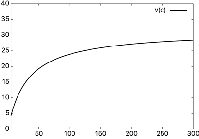
Figure 2: Average RNAP velocity $v(c)$ in $bp/s$ as function of NTP concentration $c$ in $\mu M$ at amplitude value $A(\rho,y)=1$.

By using an excess of DNA one can regulate the number of RNAP initiating from a single DNA molecule and thus the RNAP density. We consider first the predictions for minimal interaction range. As a function of the density, the speed increases and reaches maximum at $\rho^{\ast}>0$ only if $y>2$. This can be shown analytically by taking the derivative of (3.22) w.r.t. the density. Thus, while stochastic pushing always occurs in single jumps, it has a cooperative effect on the avarage speed of a single RNAP in an ensemble of interacting RNAP only for sufficiently strong repulsion, up to some characteristic blocking density $\rho_{b}$ above which blocking dominates and the velocity drops below that of an isolated RNAP without pushing. Weak short-range repulsion below the critical value (or attraction) reduce the speed of the RNAP as the density increases, as does pure hard-core repulsion. Hence this regime is blocking-dominated, i.e., the pushing effect is not strong enough to compensate the blocking due to steric hard-core repulsion. These features are shown in Fig. 3, left panel.

In contrast, the total average elongation rate $j=\rho v$ increases for any interaction strength, even for attractive interaction. It reaches a maximum at a second critical density $\rho^{\ast\ast}>\rho^{\ast}$ (Fig. 3, right panel) where for $y\leq 2$ we define $\rho^{\ast}=0$. However, cooperativity sets in again only above the critical repulsion strength $y_{c}=2$. Otherwise the flux of interacting RNAP is lower than the flux generated by the same number of single RNAP (dotted curve in the right panel). We stress that pushing is not an input in our calculation of the transition rates, but is a prediction borne out by experiments.

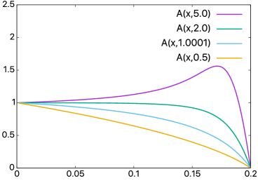
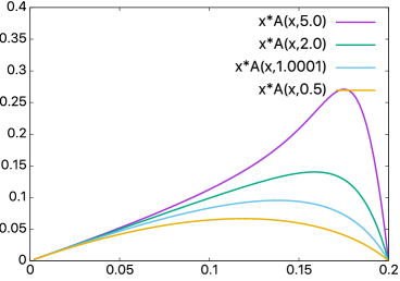
Figure 3: RNAP velocity amplitude $A(\rho,y)$ (left panel) and RNAP flux amplitude $\rho A(\rho,y)$ (right panel) as function of RNAP density for different interaction strengths $y$ and minimal interaction range. Curves from top to bottom: $y=5.0$ (strong repulsion), $y=2.0$ (critical repulsion strength), $y=1.0001$ (only hard core), $y=0.5$ (attraction). The dotted reference line corresponds to non-interacting RNAP.

Next we point out our predictions for situations where experimental results are currently not available. We consider manipulating the kinetic interaction range which may be probed by applying an external torque to the RNAP, as has been suggested as a means to to regulate the average velocity of RNAP [39]. Taking in (3.27) the derivative w.r.t. the density at density 0 one finds that the average speed increases with density provided that

$$d^{1\star}>-1/2+y^{-1}.$$ (3.29)

Since $d^{\star 1}<0$ (stochastic blocking enhancement) is assumed, cooperative pushing at low densities requires the same minimal interaction strength $y_{c}=2$ as in the case of minimal interaction range.

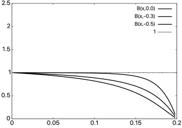
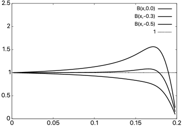
Figure 4: RNAP velocity amplitude $B(\rho,y,d^{\star 1})$ for interaction strengths $y=2$ (left panel) and $y=5$ (right panel) as function of RNAP density for different values of $d^{\star 1}$ that characterize the extended interaction range. Curves from top to bottom: $d^{\star 1}=0$ (reference curve without extension of interaction range), $d^{\star 1}=-0.3$ (intermediate blocking enhancement), $d^{\star 1}=-0.5$ (critical blocking enhancement). The dotted reference line corresponds to non-interacting RNAP.

In terms of the interaction parameters $d^{1\star},d^{\star 1}>-1$ the limiting curve (3.29) is in the domain $d^{\star 1}>-1/2$, $d^{1\star}>0$. This has a twofold meaning. First, stochastic pushing ($d^{1\star}>0$) is necessary for cooperative pushing to emerge. When the stochastic blocking enhancement is too strong ($d^{\star 1}\leq d^{\star 1}_{c}=-1/2$), then even strong stochastic pushing ($y$ arbitrarily large) does not lead to cooperative pushing at low densities. In Fig. 4 these effects are illustrated by for $y=y_{c}$ (left panel, no cooperative pushing at any density) and for strong repulsion $y=5$ (right panel, cooperative pushing until jamming takes over at high density, provided stochastic blocking enhancement is not too strong ($d^{1\star}>0.3$).

When both repulsive static interaction and stochastic blocking enhancement are very strong, a new phenomenon appears. The speed of an RNAP develops an intermediate minimum at a density $\rho_{m}$. The local minimum deepens with increasing static repulsion and is outside the range of cooperative pushing, even though there is stochastic pushing. Somewhat paradoxically, however, at higher densities there a reentrance to a cooperative pushing regime, see Fig. 5 for two different values of $y$. For a range of densities stochastic pushing prevails over stochastic blocking enhancement. Only at very high densities cooperative pushing disappears again. The drop is also present in the average elongation rate at a higher density, see Fig. 6 where the velocity amplitude $B(\rho,y,d^{\star 1})$ (left panel) and the flux amplitude $\rho B(\rho,y,d^{\star 1})$ (right panel) are shown for a large value $y=50$ of the static repulsion strength. The large value was chosen to demonstrate that the reentrance effect can be very pronounced and is very sensitive to the interaction parameter $d^{\star 1}$.

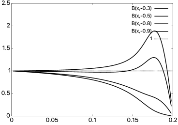
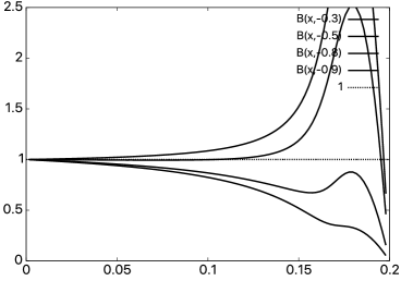
Figure 5: RNAP velocity amplitude $B(\rho,y,d^{\star 1})$ for large interaction strengths $y=10$ (left panel) and $y=20$ (right panel) as function of RNAP density for different values of $d^{\star 1}$. Curves from top to bottom: $d^{\star 1}=-0.3,-0.5,-0.8,-0.9$. The dotted reference line corresponds to non-interacting RNAP.

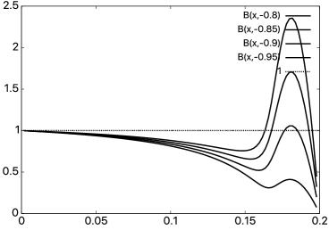
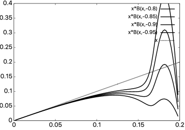
Figure 6: RNAP velocity amplitude $B(\rho,y,d^{\star 1})$ (left panel) and flux amplitude (right panel) for large interaction strength $y=50$ as function of RNAP density for different values of $d^{\star 1}$. Curves from top to bottom: $d^{\star 1}=-0.8,-0.85,-0.9,-0.95$. The dotted reference line corresponds to non-interacting RNAP.

4 Conclusions

The elongation phase can involve multiple RNAPs moving one after another along the same DNA molecule. Therefore an investigation of the kinetics of transcription requires taking into account interactions between RNAP. Experimental results that demonstrate a pushing effect of trailing RNAP necessitate a description of such interactions that goes beyond a steric hard-core repulsion through additional short-range interactions. To our knowledge the approach developed in this paper is the first attempt to capture such extra interactions as well as the mechanochemical cycles of each individual RNAP in the elongation stage in a stochastic model that allows for an exact analytical computation of its stationary properties. In particular, we make precise predictions on the average rate of elongation as a function of interaction strength as well as the RNAP density and NTP concentration which can be manipulated experimentally so that model predictions can be tested.

The model is based on a reduced picture of the mechanochemical cycle and incorporates a nearest-neighbour interaction that allows us to understand certain qualitative and quantitative aspects of the kinetics of transcription and the dependence of the rate of elongation on interactions. Without using the experimental results on pushing in the computation of the transition rates, the model predicts pushing: When a trailing RNAP reaches a paused RNAP, then the paused RNAP continues stochastically with a higher translocation rate as in the absence of the trailing RNAP. A stationary distribution for RNAP with hard-core repulsion only is not compatible with any kinetic mechanism that produces the experimentally observed pushing phenomenon. This mechanism requires an RNAP distribution that incorporates an additional static short-range repulsion.

However, according to the model, the cooperative effect of individual RNAP pushing, i.e, the enhancement of the average elongation rate, requires an effective short-range repulsion between RNAP beyond a certain strength. Given this interaction strength, cooperative pushing persists up to a maximal RNAP density beyond which jamming due to hard-core repulsion prevails. At such high RNAP densities the elongation rate of multiple RNAP transcribing on the same DNA segment is reduced compared to the same number of non-interacting RNAP, i.e., an average over RNAP transcribing the same RNA independently on different DNA molecules.

A second outcome of our approach is a certain degree of freedom in the choice of kinetic processes that do not alter the stationary distribution. In particular, one can describe not only pushing, but also a stochastic blocking enhancement that goes beyond the effects of pure hard-core repulsion by a reduction of the translocation rate when a trailing RNAP approaches a paused RNAP. At present there are not sufficient experimental data for any specific RNAP to determine these parameters. For the sake of simplicity, we have illustrated the effect of the interplay of stochastic pushing and stochastic blocking enhancement for the simplest case compatible with stationarity of the RNAP distribution.

It turns out that the RNAP velocity and transcription rate are sensitive to this interplay in a subtle and somewhat surprising manner. At low densities and moderately strong repulsion cooperative pushing occurs much in the same way as without stochastic blocking enhancement, provided that stochastic blocking enhancement is not too strong. When stochastic blocking enhancement is very strong, then a moderate stochastic pushing is not sufficient to generate a cooperative pushing effect. However, when also the repulsion (and therefore stochastic pushing) is very strong then as RNAP density increase, the elongation rate first decreases (due to jamming), but it reaches a minimum and then enters a range of RNAP density, where cooperative pushing reappears. Only at very high RNAP density jamming dominates again.

Thus the model provides an explanation of cooperative pushing in terms of static and kinetic interactions between neighbouring RNAP. The modelling approach is mathematically robust and can be extended to allow for a more detailed biological description of the mechanochemical cycle of the RNAP during elongation, for back-tracking, and also for incorporating more general short-range interactions.

5 Acknowledgements

G.M.S. thanks the Instituto de Matemática e Estatástica of the University of São Paulo for kind hospitality. This work was financed in part by Coordenação de Aperfeiçoamento de Pessoal de Nível Superior – Brazil (CAPES) – Finance Code 001, by the grants 2017/20696-0, 2017/10555-0 of São Paulo Research Foundation (FAPESP), and by the grant 309239/2017-6 of Conselho Nacional de Desenvolvimento Cinetífico e Tecnológico (CNPq). The authors thank D. Chowdhury (IIT Kanpur) for useful comments on an early draft of this paper.

Appendix A Mapping to the headway process

We consider the extended interaction range. All results for minimal interaction range follow by taking $d^{\star 1}=f^{10\star}=f^{\star 01}=0$.

A.1 Master equation and stationary distribution

Because of translation invariance one may describe the RNAP model in terms of the headway distances $\mathbf{m}=(m_{1},\dots,m_{N})$ with $m_{i}=x_{i+1}-(x_{i}+\ell)\bmod L$ which is the number of vacant sites between the left edge of rod $i+1$ and the right edge of rod $i$. The total number of vacant sites is $M=L-N$. It is convenient to introduce the indicator functions

$$\theta_{i}^{p}:=\delta_{m_{i},p}=\delta_{x_{i+1},x_{i}+\ell+p}$$ (A.1)

on a headway of length $p$ (in units of bp) with the index $i$ taken modulo $N$, i.e., $\theta_{0}^{p}\equiv\theta_{N}^{p}$. Since $\theta_{i}^{p}$ takes only values 0 or 1 one has

$$y^{\theta_{i}^{p}}=1+(y-1)\theta_{i}^{p}$$ (A.2)

which is useful for explicit computations.

A translocation of RNAP $i$ corresponds to the transition

$$(m_{i-1},m_{i})\to(m_{i-1}+1,m_{i}-1)$$

with all other distances remaining unchanged. Due to steric hard-core repulsion this transition can only take place if $m_{i}>0$. In terms of the new stochastic variables $\boldsymbol{\zeta}=(\mathbf{m},\mathbf{s})$ given by the distance vector $\mathbf{m}$ and the state vector $\mathbf{s}$ the transition rates (2.11) and (2.12) for extended interaction range become

$$\tilde{\omega}_{i}(\boldsymbol{\zeta}) = \omega^{\star}\delta_{s_{i},1}\left(1-\theta^{0}_{i}\right)\left(1+d^{1\star}\theta^{0}_{i-1}+d^{\star 1}\theta^{1}_{i}\right)$$ (A.3)

$$\tilde{\kappa}_{i}(\boldsymbol{\zeta}) = \kappa^{\star}\delta_{s_{i},2}\left(1+f^{1\star}\theta^{0}_{i-1}+f^{\star 1}\theta^{0}_{i}+f^{1\star 1}\theta^{0}_{i-1}\theta^{0}_{i}+f^{10\star}\theta^{1}_{i-1}+f^{\star 01}\theta^{1}_{i}\right).$$ (A.4)

In the mapping to the headway process the stationary average speed of an RNAP is given by the stationary expectation of the function $\tilde{\omega}_{i}(\boldsymbol{\zeta})$.

In order to write the master equation we need to introduce notation for the configurations that lead to a given configuration $\boldsymbol{\zeta}$, viz. $\boldsymbol{\zeta}^{i-1,i}$ for translocation and $\boldsymbol{\zeta}^{i}$ for PP_i release. For a fixed $\boldsymbol{\zeta}$ these configurations are defined by

$$\mathbf{s}^{i-1,i}_{j}=\mathbf{s}_{j}+(3-2s_{j})\delta_{j,i},\quad\mathbf{m}^{i-1,i}_{j}=m_{j}+\delta_{j,i}-\delta_{j,i-1}$$ (A.5)

$$\mathbf{s}^{i}_{j}=\mathbf{s}_{j}+(3-2s_{j})\delta_{j,i},\quad\mathbf{m}^{i}_{j}=m_{j}.$$ (A.6)

This yields the master equation

$$\frac{\mathrm{d}}{\mathrm{d}t}P(\boldsymbol{\zeta},t)=\sum_{i=1}^{N}Q_{i}(\boldsymbol{\zeta},t)$$ (A.7)

with

$$Q_{i}(\boldsymbol{\zeta},t) = \tilde{\omega}_{i}(\boldsymbol{\zeta}^{i-1,i})P(\boldsymbol{\zeta}^{i-1,i},t)-\tilde{\omega}_{i}(\boldsymbol{\zeta})P(\boldsymbol{\zeta},t)$$ (A.8)

$$+\tilde{\kappa}_{i}(\boldsymbol{\zeta}^{i})P(\boldsymbol{\zeta}^{i},t)-\tilde{\kappa}_{i}(\boldsymbol{\zeta})P(\boldsymbol{\zeta},t).$$

This is the master equation for a misanthrope process [40] generalized to sites $i$ that can take two degrees of freedom $s_{i}$.

An important property of the stationary distribution (2.3) is the independence of the probability to find an RNAP in state 1 or 2 from the spatial distribution of RNAPs. An immediate consequence is the factorization of the partition function (2.5) into into a summation over states and a summation over the spatial degrees of freedom. Thus one finds for the stationary distribution in terms of the parameters (2.7) and the new distance variables (A.1) the expression

$$\tilde{\pi}(\boldsymbol{\zeta})=\frac{1}{Z}\prod_{i=1}^{N}\left(y^{-\theta_{i}^{0}}x^{-3/2+s_{i}}\right)$$ (A.9)

which is of factorized form, indicating the absence of distance correlations.

A.2 Proof of stationarity

Notice that in the stationary state the master equation (A.7) has the form of a conservation law $\dot{Q}=0$ where $Q=\sum_{i}Q_{i}$ with a locally conserved stationary quantity $Q_{i}$. Invoking the discrete form of the Noether theorem leads us to conclude that there is a locally conserved current $J_{i}$ associated with $Q_{i}$ such that one can write $Q_{i}=J_{i-1}-J_{i}$. Defining

$$\tilde{D}_{i}(\boldsymbol{\zeta}) = \tilde{\omega}_{i}(\boldsymbol{\zeta}^{i-1,i})\frac{\tilde{\pi}(\boldsymbol{\zeta}^{i-1,i})}{\tilde{\pi}(\boldsymbol{\zeta})}-\tilde{\omega}_{i}(\boldsymbol{\zeta})$$ (A.10)

$$\tilde{F}_{i}(\boldsymbol{\zeta}) = \tilde{\kappa}_{i}(\boldsymbol{\zeta}^{i})\frac{\tilde{\pi}(\boldsymbol{\zeta}^{i})}{\tilde{\pi}(\boldsymbol{\zeta})}-\tilde{\kappa}_{i}(\boldsymbol{\zeta})$$ (A.11)

one gets $Q_{i}=(\tilde{D}_{i}+\tilde{F}_{i})\pi^{-1}$. We can therefore rephrase the stationarity condition in a local divergence form equivalent to (3.11) with a locally conserved current $J_{i}=\tilde{\Phi}_{i}\pi$.

One has

$$\theta_{j}^{p}(\boldsymbol{\zeta}^{i-1,i})=\delta_{m_{j}+\delta_{j,i}-\delta_{j,i-1},p}=\theta_{j}^{p-\delta_{j,i}+\delta_{j,i-1}}(\boldsymbol{\zeta}),\quad\delta_{s^{i}_{i},\alpha}=\delta_{2s_{i},3-\alpha}$$ (A.12)

which yields

$$\frac{\tilde{\pi}(\boldsymbol{\zeta}^{i-1,i})}{\tilde{\pi}(\boldsymbol{\zeta})} = x^{3-2s_{i}}y^{\theta_{i-1}^{0}+\theta_{i}^{0}-\theta_{i-1}^{1}}$$ (A.13)

$$\tilde{\omega}_{i}(\boldsymbol{\zeta}^{i-1,i}) = \omega^{\star}\delta_{s_{i},2}\left(1-\theta^{0}_{i-1}\right)\left(1+d^{1\star}\theta^{1}_{i-1}+d^{\star 1}\theta^{0}_{i}\right)$$ (A.14)

and therefore

$$\tilde{D}_{i}(\boldsymbol{\zeta}) = x^{-1}\omega^{\star}\delta_{s_{i},2}\left(1-\theta^{0}_{i-1}\right)\left(1+d^{1\star}\theta^{1}_{i-1}+d^{\star 1}\theta^{0}_{i}\right)y^{\theta_{i}^{0}-\theta_{i-1}^{1}}$$ (A.15)

$$-\omega^{\star}\delta_{s_{i},1}\left(1-\theta^{0}_{i}\right)\left(1+d^{1\star}\theta^{0}_{i-1}+d^{\star 1}\theta^{1}_{i}\right)$$

$$\tilde{F}_{i}(\boldsymbol{\zeta}) = \left(x\delta_{s_{i},1}-\delta_{s_{i},2}\right)$$ (A.16)

$$\times\kappa^{\star}\left(1+f^{1\star}\theta^{0}_{i-1}+f^{\star 1}\theta^{0}_{i}+f^{1\star 1}\theta^{0}_{i-1}\theta^{0}_{i}+f^{10\star}\theta^{1}_{i-1}+f^{\star 01}\theta^{1}_{i}\right)$$

One notices that $\tilde{D}_{i}$ and $\tilde{F}_{i}$ depend only on the state at site $i$ and only on the distance variables $\theta^{0}_{i-1}$, $\theta^{1}_{i-1}$, $\theta^{0}_{i}$, and $\theta^{1}_{i}$. This implies that the local divergence conditions holds (3.11) if and only if

$$\tilde{D}_{i}+\tilde{F}_{i}=\tilde{\Phi}_{i-1}-\tilde{\Phi}_{i}$$

where the quantity $\tilde{\Phi}_{i}$ is of the form $\tilde{\Phi}_{i}=a+b\theta^{0}_{i}+c\theta^{1}_{i}$ with arbitrary constants $a,b,c$. This fact imposes conditions on the interaction parameters appearing in (A.15) and (A.16) which are obtained by requiring

$$\tilde{D}_{i}+\tilde{F}_{i}=[(a+b\theta^{0}_{i-1}+c\theta^{1}_{i-1})-(a+b\theta^{0}_{i}+c\theta^{1}_{i})](\delta_{s_{i},1}+\delta_{s_{i},2}).$$

Comparing in (A.15) and (A.16) the constant terms (independent of $\theta^{\alpha}_{i-1}$ and $\theta^{\alpha}_{i}$) one finds $a=0$ and (3.1). Comparing all the remaining terms proportional to $\delta_{s_{i},1}$ one finds the relation (3.5) and

$$f^{1\star}+f^{\star 1}=d^{1\star}-1$$ (A.17)

$$f^{10\star}+f^{\star 01}=d^{\star 1}$$ (A.18)

corresponding to $b=f^{1\star}-d^{1\star}$ and $c=f^{10\star}$. Finally, using these preliminary results and comparing each term in (A.15) and (A.16) proportional to $\delta_{s_{i},2}$ to the corresponding term proportional to $\delta_{s_{i},1}$ by using the indicator property (A.2) one arrives after some straightforward computation at the relations (3.2), (3.3), (3.4), (3.6), and (3.7). This completes the proof of stationarity.

A.3 Partition function

It is convenient to work in the grandcanonical ensemble defined by

$$\tilde{\pi}_{gc}(\boldsymbol{\zeta})=\frac{1}{Z_{gc}}\prod_{i=1}^{N}\left(z^{m_{i}}y^{-\theta_{i}^{0}}x^{-3/2+s_{i}}\right)$$ (A.19)

where $Z_{gc}=(Z_{1}Z_{2})^{N}$ with

$$Z_{1}=\frac{1+(y-1)z}{1-z},\quad Z_{2}=x^{\frac{1}{2}}+x^{-\frac{1}{2}}.$$ (A.20)

From this grandcanonical distribution one obtains the mean headway

$$\mbox{$\langle\,{m_{i}}\,\rangle$}=z\frac{\mathrm{d}}{\mathrm{d}z}\ln Z_{gc}=\frac{yz}{(1-z)(1+(y-1)z)}.$$ (A.21)

On the other hand, this is the mean available empty space on the lattice $L-\ell N$ per rod which gives $\mbox{$\langle\,{m_{i}}\,\rangle$}=\frac{1}{\rho}-\ell$ where

$$\rho=\frac{N}{L}$$ (A.22)

is the RNAP density. Hence the auxiliary variable $z$ is the solution of the quadratic equation

$$(y-1)z^{2}+z\left(\frac{y\rho}{1-\ell\rho}-y+2\right)-1=0$$ (A.23)

given by

$$z(\rho,y)=1-\frac{1-(\ell-1)\rho-\sqrt{(1-(\ell-1)\rho)^{2}-4\rho(1-\ell\rho)(1-y^{-1})}}{2(1-\ell\rho)(1-y^{-1})}.$$ (A.24)

Notice that the model allows for a number density in the range $0<\rho\leq 1/\ell$. This ensures that $0\leq z<1$ and therefore the partition function (A.19) is well-defined.

References

- [1] Alberts, B., D. Bray, K. Hopkin, A. Johnson, J. Lewis, M., K. Roberts, and P. Walter. 2013. Essential Cell Biology. 4th ed., Garland Science, New York.
- [2] Bai, L., T. J. Santangelo, and M. D. Wang. Single-Molecule Analysis of RNA Polymerase Transcription. 2006. Annu. Rev. Biophys. Biomol. Struct. 35:343–360
- [3] Ma, C., X. Yang, and P. J. Lewis. 2016. Bacterial transcription as a target for antibacterial drug development. Microbiol. Mol. Biol. Rev. 80:139–160.
- [4] Guthold, M. X. Zhu, C. Rivetti, G. Yang, N. H. Thomson, S. Kasas, H. G. Hansma, B. Smith, P. K. Hansma, and C.s Bustamante. 1999. Direct Observation of One-Dimensional Diffusion and Transcription by Escherichia coli RNA Polymerase. Biophys. J. 77:2284–2294
- [5] Ó Maoiléidigh, D., V. R. Tadigotla, E. Nudler, and A. E. Ruckenstein. 2011. A Unified Model of Transcription Elongation: What Have We Learned from Single-Molecule Experiments? Biophys. J. 100:1157–1166.
- [6] Wang, H. Y. , T. Elston, A. Mogilner, and G. Oster. 1998. Force Generation in RNA Polymerase. Biophys. J. 74:1186–1202.
- [7] Wu, S., L. Li, and Q. Li. 2017. Mechanism of NTP Binding to the Active Site of T7 RNA Polymerase Revealed by Free-Energy Simulation, Biophys. J. 112:2253–2260.
- [8] Da L-T, E C, Duan B, Zhang C, Zhou X, Yu J (2015) A Jump-from-Cavity Pyrophosphate Ion Release Assisted by a Key Lysine Residue in T7 RNA Polymerase Transcription Elongation. PLoS Comput. Biol. 11:e1004624.
- [9] Mejia, Y. X., E. Nudler, and C. Bustamante. 2015. Trigger loop folding determines transcription rate of Escherichia coli’s RNA polymerase. Proc. Natl. Acad. Sci. USA 112:743–748
- [10] Zhang, L., F. Pardo-Avila, I. C. Unarta, P. P.-H. Cheung, G. Wang, D. Wang, and X. Huang. 2016. Elucidation of the Dynamics of Transcription Elongation by RNA Polymerase II using Kinetic Network Models. Acc. Chem. Res., 49:687–694.
- [11] Klumpp, S., and T. Hwa. 2008. Stochasticity and traffic jams in the transcription of ribosomal RNA: Intriguing role of termination and antitermination. Proc. Natl. Acad. Sci. USA 105:18159–18164.
- [12] T. Tripathi, and D. Chowdhury. 2008. Interacting RNA polymerase motors on a DNA track: Effects of traffic congestion and intrinsic noise on RNA synthesis. Phys. Rev. E 77:011921.
- [13] Tripathi, T., G. M. Schütz, and D. Chowdhury. 2009. RNA polymerase motors: dwell time distribution, velocity and dynamical phases. J. Stat. Mech 2009:P08018.
- [14] Epshtein, V., and E. Nudler. 2003. Cooperation between RNA polymerase molecules in transcription elongation. Science 300:801–805.
- [15] Epshtein, V., F. Toulme, A. Rachid Rahmouni, S. Borukhov, and E. Nudler. 2003. Transcription through the roadblocks: the role of RNA polymerase cooperation. EMBO J. 22:4719–4727 .
- [16] Saeki, H., and J. Q. Svejstrup. 2009. Stability, flexibility, and dynamic interactions of colliding RNA polymerase II elongation complexes. Mol. Cell. 35:191–205.
- [17] Jin, J., L. Bai, D. S. Johnson, R.M. Fulbright, M.L. Kireeva, M. Kashlev, and M.D. Wang. 2010. Synergistic action of RNA polymerases in overcoming the nucleosomal barrier. Nat. Struct. Mol. Biol. 17:745–752.
- [18] Ehrenberg, M., P.P. Dennis, and H. Bremer. 2010. Maximum rrn promoter activity in Escherichia coli at saturating concentrations of free RNA polymerase. Biochimie 92: 12–20.
- [19] Galburt, E.A., J. M..R. Parrondo, and S. W. Grill. 2011. RNA polymerase pushing. Biophys. Chem. 157:43–47.
- [20] Klumpp, S. 2011. Pausing and backtracking in transcription under dense traffic conditions. J. Stat. Phys. 142:1252–1267.
- [21] Schadschneider, A., D. Chowdhury and K. Nishinari. 2010. Stochastic Transport in Complex Systems. Elsevier, Amsterdam.
- [22] Costa, P.R., M.L. Acencio, and N. Lemke. 2013. Cooperative RNA Polymerase Molecules Behavior on a Stochastic Sequence-Dependent Model for Transcription Elongation. PLoS ONE 8(2): e57328.
- [23] L. Bai, A. Shundrovsky, and M.D. Wang. 2004. Sequence-dependent kinetic model for transcription elongation by RNA polymerase. J. Mol. Biol. 344: 335–349.
- [24] Bai, L., R. M. Fulbright, and M. D. Wang. 2007. Mechanochemical kinetics of transcription elongation. Phys. Rev. Lett. 98:068103.
- [25] Teimouri, H., A. B. Kolomeisky, and K. Mehrabiani. 2015. Theoretical Analysis of Dynamic Processes for Interacting Molecular Motors. J. Phys. A: Math. Theor. 48: 065001.
- [26] Heberling, T., L. Davis, J. Gedeon, C. Morgan, and T. Gedeon. 2016. A Mechanistic Model for Cooperative Behavior of Co-transcribing RNA Polymerases. PLoS Comput. Biol. 12: e1005069.
- [27] Yin, H., M. D. Wang, K. Svoboda, R. Landick, S. M. Block, and J. Gelles. 1995. Transcription against an applied force. Science 270:1653–1657.
- [28] Erie, D. A., T. D. Yager, and P. von Hippel. 1992. The single-nucleotide addition cycle in transcription: a biophysical and biochemical perspective. Annu. Rev. Biophys. Biomol. Struct. 21:379–415.
- [29] Geszvain K., and R. Landick. 2005. The structure of bacterial RNA polymerase. In The bacterial chromosome. P. Higgins, editor. ASM, Washington, pp 283–296.
- [30] MacDonald, J.T., J.H. Gibbs, and A.C. Pipkin. 1968. Kinetics of biopolymerization on nucleic acid templates. Biopolymers 6:1–25.
- [31] Shaw, L.B., R. K. P. Zia, and K. H. Lee. 2003. Totally asymmetric exclusion process with extended objects: A model for protein synthesis. Phys. Rev. E 68:021910
- [32] Klumpp, S. and R. Lipowsky. 2003. Traffic of Molecular Motors Through Tube-Like Compartments. J. Stat. Phys. 113: 233–268.
- [33] Chou, T. and G. Lakatos. 2004. Clustered bottlenecks in mRNA translation and protein synthesis. Phys. Rev. Lett. 93:198101.
- [34] Frey, E., A. Parmeggiani, and T. Franosch. 2004. Collective Phenomena in Intracellular Processes. Genome Inf. 15:46–55
- [35] Dong, J.J., B. Schmittmann, B. and R.K.P. Zia. 2007. Towards a Model for Protein Production Rates J. Stat. Phys. 128: 21–34.
- [36] Greulich, P., A. Garai, K. Nishinari, A. Schadschneider, and D. Chowdhury. 2007. Intracellular transport by single-headed kinesin KIF1A: Effects of single-motor mechanochemistry and steric interactions Phys. Rev. E 75:041905.
- [37] Kolomeisky, A.B., and M. E. Fisher. 2007. Molecular Motors: A Theorist’s Perspective. Annu. Rev. Phys. Chem. 58:675–95
- [38] Chowdhury, D. 2013. Stochastic mechano-chemical kinetics of molecular motors: A multidisciplinary enterprise from a physicist’s perspective. Phys. Rep. 529:1–197.
- [39] Tripathi, T., P. Prakash, D. Chowdhury. 2008. RNA polymerase motor on DNA track: effects of interactions, external force and torque. arXiv:0812.4692.
- [40] Cocozza-Thivent, C. 1985. Processus des misanthropes, Z. Wahrsch. Verw. Gebiete 70:509–523.