Analysis and Performance Evaluation of Adjoint-Guided Adaptive Mesh Refinement for Linear Hyperbolic PDEs Using Clawpack

Abstract.

Adaptive mesh refinement (AMR) is often used when solving time-dependent partial differential equations using numerical methods. It enables time-varying regions of much higher resolution, which can be used to track discontinuities in the solution by selectively refining around those areas. The open source Clawpack software implements block-structured AMR to refine around propagating waves in the AMRClaw package. For problems where the solution must be computed over a large domain but is only of interest in a small area this approach often refines waves that will not impact the target area. We seek a method that enables the identification and refinement of only the waves that will influence the target area.

Here we show that solving the time-dependent adjoint equation and using a suitable inner product allows for a more precise refinement of the relevant waves. We present the adjoint methodology in general, and give details on how this method has been implemented in AMRClaw. Examples for linear acoustics equations are presented, and a computational performance analysis is conducted. The adjoint method is compared to AMR methods already available in the AMRClaw software, and the resulting advantages and disadvantages are discussed. The code for the examples presented is archived on Github.

1. Introduction

Hyperbolic systems of partial differential equations appear in the study of numerous physical phenomena involving wave propagation. Methods for numerically calculating solutions to these systems of PDEs have broad applications in many disciplines. Complicating the development of numerical methods for solving these systems is the fact that solutions often contain discontinuities or localized steep gradients. A variety of adaptive mesh refinement (AMR) techniques have been developed to allow the use of much finer grids around discontinuities or localized regions needing higher resolution, which generally propagate as the solution evolves. Nonlinear hyperbolic problems that produce shock waves often require AMR in regions that can be easily identified by computing the local gradient. But AMR is often also extremely useful for linear hyperbolic equations with smooth solutions, particularly when the solution is of interest over some small region relative to the size of the computational domain. Examples motivating this work include modeling tsunami propagation over the ocean (for which linearized shallow water equations are suitable until the waves reach shore) and earthquake modeling, where linear elasticity equations are generally used. In both cases spatially varying coefficients in the PDE lead to scattering and reflections that can make it difficult to predict which portions of the domain must be refined at any given time in order to capture the waves that will ultimately reach the location of interest.

We present a general approach to using the adjoint equation to efficiently guide adaptive refinement in this situation, and describe an implementation of this approach in the Clawpack software (Clawpack Development Team, 2015; Mandli et al., 2016). This open source software has been developed since 1994 and can be applied to almost any hyperbolic PDE in 1, 2, or 3 space dimensions by providing a Riemann solver, the basic building block of the high-resolution Godunov-type finite volume methods that are employed (Bale et al., 2002; Langseth and LeVeque, 2000; LeVeque, 1997, 2004). The AMRClaw package of Clawpack uses block structured AMR as developed in (Berger and Oliger, 1984; Berger and Colella, 1989) and adapted to the wave-propagation algorithms used in Clawpack in (Berger and LeVeque, 1998). The AMR software is also used in the GeoClaw variant of Clawpack developed for modeling tsunamis, storm surge, and other geophysical flows (e.g. (Berger et al., 2011; LeVeque et al., 2011; Mandli and Dawson, 2014)).

For a hyperbolic PDE, the adjoint equation is another (closely related) hyperbolic PDE that must be solved backwards in time, starting with a disturbance at the location of interest. Waves propagating outward in this adjoint solution indicate the portion of the domain that can affect the solution at the location and time of interest. Taking a suitable inner product between the forward solution (or an estimate of the local error in the forward solution) and the adjoint solution allows us to determine what regions need to be refined at each earlier time.

We concentrate on linear (variable coefficient) problems in this paper because in this case the adjoint equation is independent of the forward solution, and can be computed a priori before solving the forward problem. The adjoint problem is generally solved on a much coarser grid than will be used for the forward problem, so that this adds relatively little computational expense. For a nonlinear hyperbolic PDE an adjoint problem can still be defined, but involves linearizing about a particular solution of the forward problem. For nonlinear problems, making full use of the adjoint to guide adaptive refinement might require iterating between approximations to the forward and adjoint problem as the forward problem is better resolved in appropriate regions. The work reported in this paper could form the basis for such an extension, and has already proved very useful in its own right for the applications mentioned above. We also assume that the coefficients vary in space but not in time. Time-varying coefficients could be handled in much the same way if the focus is on a single output time of interest, but in most practical cases the coefficients are time-invariant and hence the equation is autonomous in time. This makes it easy to extend the approach to handle problems where the solution at one spatial location is of interest over a range of times, which is the situation in the examples mentioned above, for example. The adjoint solution needs to be computed only once over a sufficiently long time period, and snapshots in time of this one solution can be used to guide the adaptive refinement regardless of the time period of interest.

In two space dimensions (with obvious modifications for 1 or 3 dimensions), a linear hyperbolic system with coefficients varying in space typically takes one of two forms, either the conservative form

(1) $$q_{t}(x,y,t)+(A(x,y)q(x,y,t))_{x}+(B(x,y)q(x,y,t))_{y}=0,$$

or the non-conservative form

(2) $$q_{t}(x,y,t)+A(x,y)q_{x}(x,y,t)+B(x,y)q_{y}(x,y,t)=0.$$

Of course eq:hypsys_nonconserv differs from eq:hypsys_conserv only if the coefficient matrices vary in space. Often the same physical system can be modeled by equations of either form, depending on what variables are chosen to make up the vector $q(x,y,t)$. For example, linear acoustics can be written in the form eq:hypsys_conserv as a system of 3 equations where $q$ models small disturbances of density and momenta in the $x$- and $y$-directions. Alternatively the same acoustics problem can be modeled in the form eq:hypsys_nonconserv (with different coefficient matrices) if instead the system is written in terms of pressure and velocities. Clawpack can be used to solve equations in either form. This is important to note since if the original equation is in one form then the adjoint equation takes the other form. As derived below in sec:adjeqn, the adjoint equations arise from an integration by parts and hence if the original equation is eq:hypsys_conserv then the adjoint equation is

(3) $$\hat{q}_{t}(x,y,t)+A(x,y)^{T}\hat{q}_{x}(x,y,t)+B(x,y)^{T}\hat{q}_{y}(x,y,t)=0,$$

while if the original equation is eq:hypsys_nonconserv then the adjoint equation is

(4) $$\hat{q}_{t}(x,y,t)+(A(x,y)^{T}\hat{q}(x,y,t))_{x}+(B(x,y)^{T}\hat{q}(x,y,t))_{y}=0.$$

In this paper we first consider one-dimensional problems (one space dimension plus time) for ease of exposition and because it is informative to view the solutions in the $x$–$t$ plane in this case. The ideas extend directly to more space dimensions and we also consider two-dimensional acoustics in sec:2d_acoustics_example. While not done in the work, the ideas presented here also extend directly to three dimensions.

A key component of any AMR algorithm is the criterion for deciding which grid cells should be refined. Before this work, four different criteria were available in AMRClaw and GeoClaw for flagging cells that need refinement from one level to the next finer level. These are:

• a Richardson extrapolation error estimation procedure that compares the solution on the existing grid with the solution on a coarser grid and refines cells where this error estimate is greater than a specified tolerance,

• refining cells where the gradient of the solution (or an undivided difference of neighboring cell values) is large,

• refining cells where the surface elevation differs significantly from sea level (this refinement criteria is specific to GeoClaw for tsunami or storm surge modeling), or

• some other user-specified criterion that examines the current solution locally.

In general these approaches will flag cells for refinement anywhere that a specified refinement tolerance is exceeded, irrespective of the fact that the area of interest may be only a subregion of the full solution domain. To address this, recent versions of AMRClaw and GeoClaw also allow specifying “refinement regions,” space-time subsets of the computational domain where refinement above a certain level can be either required or forbidden. This is essential in many GeoClaw applications where only a small region along the coast (some community of interest) must be refined down to a very fine resolution (often $1/3$ arcsecond, less than 10 meters) as part of an ocean-scale simulation. In this work we focus on acoustics examples, and in that context the region of interest might be dictated by the placement of a pressure gauge or other measurement device. These AMR regions can also be used to ensure that the simulation only refines around the waves of interest. However, since the regions are user-specified, placing them optimally often requires multiple attempts and careful examination of how the solution is behaving. This generally necessitates the use of coarser grid runs for guidance, which adds computational and user time requirements. This manual guiding of AMR may also fail to capture some waves that are important. For example, a user may determine, based on a coarser grid run, that a portion of a wave is heading away from the region of interest and therefore forbid excessive refinement in that area in an effort to save computational time. However, this portion of the wave may later reflect off a distant boundary or material heterogeneity, causing it to have an unexpected impact on the region of interest.

For any problem where only a particular area of the total solution is of interest, a method that allows specifically targeting and refining the grid in regions that influence this area of interest would allow for computational savings while also ensuring that the accuracy of the solution is preserved. This challenge is the motivation for our work presented here.

When solving the original time-dependent PDE, which we will call the “forward problem”, generally we have initial data specified at some initial time $t_{0}$ and the problem is solved forward in time to find the solution at the target location at some later time $t_{f}$ (or, more typically, over some time range of interest). The adjoint equation (derived in sec:adjeqn) must then be solved backwards in time from the final time $t_{f}$ to the initial time $t_{0}$. The “initial ” data for the adjoint equation, which must be specified at the final time, is non-zero at the target location and then spreads out into waves as the adjoint equation is solved. The key idea is that at any intermediate “regridding” time $t_{r}$, between $t_{0}$ and $t_{f}$, the only regions in space where the forward solution could possibly affect the target location at time $t_{f}$ are regions where the adjoint solution is nonzero. Moreover, by computing a suitable inner product of the forward and adjoint solutions at time $t_{r}$ it is possible to determine whether the forward solution at a given spatial point will actually impact the target location at the final time $t_{f}$, or whether it can be safely ignored. Alternatively, by computing a suitable inner product of an error estimate in the forward solution and the adjoint solution at time $t_{r}$, it is possible to estimate how much the error at a given spatial point will affect the final accuracy at the target location. This information can then be used to decide whether or not to refine this spatial location in the forward solution.

1.1. Previous Work in the Literature

The idea of using adjoint equations to guide computations has been around for many years. For an overview of the various fields in which adjoints have been utilized see (Davis and LeVeque, 2016). Historically the adjoint method has been commonly used to improve the accuracy of a solution by calculating a correction term and adding it back into the solution, see for example the work of (Pierce and Giles, 2000). Adjoint equations have also been used to compute the sensitivity of the solution to changes in the input data. This has led to the adjoint equations being utilized for system control in a wide variety of applications such as shallow-water wave control (Sanders and Katopodes, 2000), optimal control of free boundary problems (Marburger, 2012), and aerodynamics design optimization (Jameson, 1988). More relevant to this current work, the adjoint method has been used in literature to guide adaptive mesh refinement. (Becker and Rannacher, 2001) used the adjoint equation to relate the global error to errors in the physical quantities of interest for the particular problem being considered, and then used these a posteriori error estimates to refine or coarsen the mesh. (Venditti and Darmofal, 2002) and (Venditti and Darmofal, 2003) have applied the same methods to compressible two-dimensional inviscid and viscous flow problems. (Park, 2004) extended the methods of (Venditti and Darmofal, 2002) to three-dimensional problems in the area of computational fluid dynamics. All of these, however, dealt with steady state problems.

Some work on using the adjoint method to guide AMR for time-dependent problems has also been done within the finite volume community. This is a more expensive problem due to the fact that there is not a single time-invariant adjoint solution but rather the problem requires computing and saving adjoint snapshots at various times. Some examples include (Kast and Fidkowski, 2013) and (Luo and Fidkowski, 2011) who use the adjoint method to guide AMR for both spatial and temporal grid refinement for the Navier-Stokes equations and (Kouhi et al., 2015) who applies this method to the compressible Euler equations. All of these examples of using the adjoint method to guide AMR work with the discrete adjoint formulation, whereas in this work we derive the continuous adjoint and then discretize this hyperbolic system using the same finite volume methods as used for the forward problem. We presented the novel use of the continuous adjoint method in the context of the shallow water equations for tsunami modeling, as well as using the adjoint method to guide adaptive mesh refinement for problems in that field, in (Davis and LeVeque, 2016). Since then, (Lacasta et al., 2018) has published work also using the continuous adjoint equations for the shallow water equations — which they used to control their internal boundary conditions. For a comprehensive comparison of the continuous and discrete adjoint formulations see (Nadarajah and Jameson, 2000).

1.2. Outline

We first introduce various methods for determining where to apply AMR in sec:flagging, some of which have been implemented in AMRClaw and GeoClaw already and some of which were newly implemented in the Clawpack framework for this work. We then present more detail on the adjoint equation and how it can be used to guide AMR in sec:adjeqn, and some specifics on implementing this new method in the context of Clawpack are presented in sec:algorithm. This basic method is expanded to take into account the approximated error in the calculated solution at each time step in sec:adjErrorFlag. Examples of this method applied to the one- and two-dimensional variable coefficient linear acoustics equations are given in sec:1d_acoustics_examples,sec:2d_acoustics_example, respectively, as well as an analysis of the computational performance of this method relative to the previously available AMR methods in Clawpack. For completeness, the appendix contains a discussion of how to solve the Riemann problem for the one-dimensional variable-coefficient acoustics problem and its adjoint.

2. Adaptive Mesh Refinement in Clawpack

The block-structured mesh refinement used in AMRClaw consists of a set of logically rectangular grid patches at multiple levels of refinement. The coarsest level contains grids that cover the entire domain, with subsequent levels representing progressively finer mesh resolutions. Generally each level is refined in both time and space to preserve the stability of the explicit finite volume method. Each level, other than the coarsest level, is properly nested within the grids that comprise the next coarsest level. For each time step on Level $L$ starting with $L=1$ for the coarsest level (and recursively applying to the finest level $L_{\max}$), the following steps are performed:

1. If $L>1$ then fill ghost cells around each patch at this level (from neighboring Level $L$ patches, or by interpolating from Level $L-1$).

2. Take a time step of length $\Delta t_{L}$ appropriate to this level.

3. If $L<L_{\max}$, then

   1. If it is time to regrid, flag cells on Level $L$ that need refining, and cluster these into rectangular patches to define the new Level $L+1$ grid patches.

   2. Take $\Delta t_{L}/\Delta t_{L+1}$ time steps on all grid patches at Level $L+1$ by recursively applying this procedure.

   3. Update the Level $L$ solution in regions covered by Level $L+1$ patches by cell-averaging the finer grid solution, and in cells directly neighboring these patches as needed to preserve conservation.

We assume the refinement ratio $\Delta t_{L}/\Delta t_{L+1}$ is an integer, generally equal to the refinement ratio in space from Level $L$ to $L+1$ in order to preserve stability, since Clawpack uses explicit finite volume methods that require the Courant number be bounded by 1. See (Berger and LeVeque, 1998) for more details on the steps above, and (Berger and Oliger, 1984; Berger and Colella, 1989) for general background on this approach. In this paper we are concerned only with step 3(a), and in particular the manner in which cells at one level are flagged for refinement to the next level. The clustering is then done using an algorithm of Berger and Rigoutsos presented in (Berger and Rigoutsos, 1991), which attempts to limit the number of unflagged cells contained in the rectangular patches while also not introducing too many separate patches. Some buffering is also done so that the refined patches extend a few grid cells out from the flagged cells. Waves can travel at most one grid cell per time step, so this ensures that waves needing refinement will not escape from the refined patches in a few time steps, but in general for a wave propagation problem it is necessary to regrid every few time steps on each level. The regridding interval and width of the buffer zone are generally related, and can each be set as input parameters in the code. Because of the need for frequent regridding, and the desire to minimize the number of needlessly refined cells, the methodology utilized for selecting which cells to flag will have a significant impact on both the accuracy of the results and the time required for the computation to run.

2.1. Flagging Methods Available in Clawpack

Prior to this work there were two built-in flagging methods available in AMRClaw, undivided differences and Richardson extrapolation. Both of these methods flag a cell if the quantity being evaluated is greater than some specified tolerance. A third flagging method, specific to GeoClaw, determines whether to flag a cell based on the surface elevation of the water. For all of the methods of refinement, if the user has specified limitations on certain regions of the domain (either requiring or forbidding flagging to occur) then these limitations are also taken into account at the flagging step in the code.

Undivided Differences. This is the default flagging routine that is used in AMRClaw. This routine evaluates the maximum max-norm of the undivided differences between a given grid cell and its two, four, or six neighbors in one, two, or three space dimensions respectively. If this maximum max-norm is greater than the specified tolerance then the cell is flagged for refinement. Therefore, this flagging method refines the mesh wherever the solution is not sufficiently smooth. This approach often works very well for problems with shock waves where the goal is to refine around all shocks. In this work, we will refer to this flagging method as difference-flagging.

Richardson Extrapolation. This second approach to flagging is based on using Richardson extrapolation to estimate the error in each cell. For each grid on Level $L$, this is done by

• advancing the current grid a time step, as normal,

• taking an extra time step on the current grid,

• generating a coarsened grid (by a factor of 2 in each direction) and taking one time step on this grid,

• comparing the solution on these two grids to estimate the one-step error introduced in a single time step with the current Level $L$ mesh size. Cells are flagged for refinement to Level $L+1$ where this estimate is above a given tolerance.

Note that this approach requires one additional time step on the Level $L$ grid and one time step on the coarsened grid, relative to difference-flagging. Therefore, it is more expensive than difference-flagging, but has the advantage of refining based on estimates of the error in the solution rather than simply anywhere that the solution is not sufficiently smooth. In this work we will refer to this flagging method as error-flagging.

2.2. Flagging Using the Adjoint Method

The adjoint-flagging method is the focus of this work. Here a very brief description of how the method can be used for AMR is given, to provide a general framework for understanding our goal for the adjoint equations. sec:adjeqn outlines the derivation of the equations required for this method, and sec:algorithm contains a detailed description of the algorithms used to implement this method. sec:adjErrorFlag expands the basic adjoint method to take into account the approximated error in the calculated solution of the forward problem at each time step. The end goal of this work is to determine which regions of the domain need to be refined at any given time by using the adjoint solution to determine what portions of the current forward solution will affect the target location.

The steps needed to use this flagging method are the following:

1. Determine the appropriate adjoint problem based on the forward problem.

2. Solve the adjoint problem backward in time, saving snapshots of the solution at various times.

3. When solving the forward problem, at each regridding time:

   1. identify the snapshot(s) of the adjoint solution that bracket the current time in the forward solution,

   2. find the value of each of the identified adjoint snapshots at the spatial location of each grid cell by interpolation,

   3. take a suitable inner product between the forward solution and each of the identified adjoint snapshots,

   4. and flag each cell if the maximum of these inner products for that grid cell is above a certain tolerance.

Note that there are several extra steps required for this flagging method, which we will refer to as adjoint-flagging, when compared to the flagging methods currently available in AMRClaw. However, much of this has been automated in the work described here, and if the adjoint problem is solved on a relatively coarse grid then the computational time added by the adjoint solution and inner products may be small relative to the time potentially saved by refining in a more optimal manner. Also note that, rather than considering the inner product between the forward problem and various selected adjoint snapshots, we could instead start from the appropriate adjoint snapshot and take a few small time steps to get to the time corresponding to the current regridding time for the forward problem. Since we are trying to minimize the amount of work required while solving the forward problem, we have selected to go with the method presented above — as it requires less computations. However, even though the method we have selected is less computationally intensive, it has proven to be extremely effective in enabling us to guide AMR for the forward problem.

Finding the appropriate adjoint problem analytically and implementing the adjoint solver is a one-time cost for each type for forward problem. For example, once the appropriate adjoint problem is found for the acoustics equations, any acoustics forward problem can use the same adjoint problem. Note that the adjoint equation is also a linear hyperbolic equation, and can therefore be solved using the same software as the forward problem. To see how this can be accomplished see sec:1d_acoustics_examples,sec:2d_acoustics_example where the adjoint problems are found for one- and two-dimensional linear acoustics problems.

When using adjoint-flagging we consider two different options when it comes to taking the inner product, stemming from a slightly different refinement criterion analogous to the difference-flagging vs. error-flagging described above.

Considering the forward solution. The first option focuses on the magnitude of the forward solution, and asks the question:

:

At a given regridding time $t_{r}$, what portions of the forward solution will eventually affect the target location?

To answer this question we take the inner product between the forward solution and the adjoint solution at the appropriate complementary time and flag the cells where this inner product is above the given tolerance. This has the advantage of flagging only cells that contain information that is pertinent to the target location and time interval, which is not possible with any of the flagging methods currently available in AMRClaw and GeoClaw. In this work we will refer to this flagging method as adjoint-magnitude flagging, which we describe in detail in sec:adjeqn,sec:algorithm. While this is often quite effective, it can be difficult to choose a suitable magnitude tolerance for flagging cells (relative to the desired accuracy of the solution). Moreover, regions where the inner product is largest do not necessarily contribute the most error to the final computed solution at the location of interest. Whether these regions actually require more refinement depends also on the smoothness of the solution and hence the accuracy of the finite volume solution.

Considering the error in the forward solution. The second option focuses on estimating the error in the forward solution, and asks the question:

:

At a given regridding time $t_{r}$, what portions of the forward solution will introduce a significant amount of error that will eventually affect the target location?

This is the question we really want to answer in deciding where to refine, but requires more work. To answer this question we estimate the one-step error in the forward solution using the Richardson extrapolation algorithm of AMRClaw, take the inner product between this error estimation and the adjoint solution at the appropriate complementary time, and flag the cells where this inner product is above a given tolerance. This method still has the advantage of flagging only cells that contain information that will reach the target location, but also only if the error estimate indicates that the error in this part of the solution is signficant on the current grid resolution. However, this flagging method is slower than adjoint-magnitude flagging because it requires the estimation of the one-step error in each grid cell using Richardson extrapolation. We will refer to this flagging method as adjoint-error flagging, and consider it further in sec:adjErrorFlag after describing the basic ideas and algorithms in the simpler context of adjoint-magnitude flagging.

3. The Adjoint Equation and Adjoint-Magnitude Flagging

For readers not familiar with the concept of an adjoint equation, (Davis and LeVeque, 2016) contains a description of the basic idea in the context of an algebraic system of equations that may be beneficial in appreciating this method, along with details of the adjoint AMR procedure and some motivating examples in the context of tsunami modeling. Here, we will present the mathematics behind finding the adjoint equation in the general context of time-dependent linear hyperbolic equations, and sec:algorithm describes the algorithms necessary to implement this method in AMRClaw and GeoClaw.

Suppose $q(x,t)$ is the solution to the time-dependent linear equation (with spatially varying coefficients)

(5) $$q_{t}(x,t)+A(x)q_{x}(x,t)=0,\quad a\leq x\leq b,\quad t_{0}\leq t\leq t_{f}$$

subject to some known initial conditions, $q(x,t_{0})$, and some boundary conditions at $x=a$ and $x=b$. Here $q(x,t)\in{{\rm l}\kern-1.49994pt{\rm R}}^{m}$ for a system of $m$ equations and we assume $A(x)\in{{\rm l}\kern-1.49994pt{\rm R}}^{m\times m}$ is diagonalizable with real eigenvalues at each $x$, so that eq:qtAqx is a hyperbolic system of equations. For the discussion and examples presented in this work we assume that we start with an equation in the form eq:hypsys_nonconserv, but we could equally well start with an equation in the form eq:hypsys_conserv.

Now suppose we do not care about the solution everywhere, but only about the value of a linear functional

(6) $$J=\int_{a}^{b}\varphi^{T}(x)q(x,t_{f})dx$$

for some given $\varphi(x)$ at the final time (or, more typically, over a range of times as considered below). Although any function $\varphi(x)$ could be specified in the method and software developed here, the case we will focus on in the examples is the common situation where we are only interested in the solution in one small spatial region (e.g., one coastal community in the case of tsunami modeling), but we need to solve the equations over a much larger region (e.g., the entire ocean) in order to determine the solution in this region. In this case it is natural to define $J$ by choosing $\varphi(x)$ to be a delta function centered at the point of interest, $\varphi(x)=\delta(x-x_{p})$. Or more realistically (and better computationally), we can take $\varphi(x)$ to be a box function or Gaussian centered about $x_{p}$ with mass 1, corresponding to $J$ being a spatial average of $q(x,t_{f})$ near the location of interest.

If $\hat{q}(x,t)\in{{\rm l}\kern-1.49994pt{\rm R}}^{m}$ is any other function then taking the inner product of $\hat{q}$ with eq:qtAqx and integrating over the space-time domain yields

(7) $$\int_{t_{0}}^{t_{f}}\int_{a}^{b}\hat{q}^{T}(x,t)\left(q_{t}(x,t)+A(x)q_{x}(x,t)\right)dx\,dt=0.$$

Then integrating by parts first in space and then in time yields the equation

(8) $$\int_{a}^{b}\left.\hat{q}^{T}q\right|^{t_{f}}_{t_{0}}dx+\int_{t_{0}}^{t_{f}}\left.\hat{q}^{T}Aq\right|^{b}_{a}dt-\int_{t_{0}}^{t_{f}}\int_{a}^{b}q^{T}\left(\hat{q}_{t}+\left(A^{T}\hat{q}\right)_{x}\right)dx\,dt=0.$$

By choosing $\hat{q}(x,t)$ to satisfiy the adjoint equation,

(9) $$\hat{q}_{t}(x,t)+(A^{T}(x)\hat{q}(x,t))_{x}=0,$$

solved backward in time from $\hat{q}(x,t_{f})=\varphi(x)$, and selecting the appropriate boundary conditions for $\hat{q}(x,t)$ such that the second integral in eq:intbyparts vanishes (which varies based on the specific system being considered), we can eliminate all terms from eq:intbyparts except the first term, to obtain

(10) $$\int_{a}^{b}\hat{q}^{T}(x,t_{f})q(x,t_{f})dx=\int_{a}^{b}\hat{q}^{T}(x,t_{0})q(x,t_{0})dx.$$

Therefore, the integral of the inner product between $\hat{q}$ and $q$ at the final time is equal to the integral at the initial time $t_{0}$:

(11) $$J=\int_{a}^{b}\hat{q}^{T}(x,t_{0})q(x,t_{0})dx.$$

Note that we can replace $t_{0}$ in eq:q_integral with any $t_{r}$ at which we wish to do regridding ($t_{0}\leq t_{r}\leq t_{f}$), which would yield eq:J with $t_{0}$ replaced by $t_{r}$. From this we observe that the locations where the inner product $\hat{q}(x,t_{r})^{T}q(x,t_{r})$ is large at the regridding time are the areas that will have a significant effect on the functional $J$. These are the areas where the solution should be refined at time $t_{r}$ if we are using adjoint-magnitude flagging. To make use of this, we must first solve the adjoint equation adjoint1 for $\hat{q}(x,t)$. This requires using “initial” data $\hat{q}(x,t_{f})=\varphi(x)$, so the adjoint problem must be solved backward in time. The strategy used for this is discussed in the next section.

4. Implementing the Adjoint Method

In principle the adjoint-flagging methodology could be used with any software that uses time-dependent AMR. In this work we are examining the specifics of implementing it in the context of AMRClaw. This section discusses the special considerations required for coding the adjoint method in Clawpack, and the resulting algorithms.

4.1. Solving the Adjoint Equation

Consider the one dimensional problem eq:qtAqx and recall that the adjoint equation adjoint1 has the form

$$\hat{q}_{t}+\left(A^{T}(x)\hat{q}\right)_{x}=0,$$

where the initial condition for $\hat{q}$ is given at the final time, $\hat{q}(x,t_{f})=\varphi(x)$, and is selected to highlight the impact of the forward solution on some region of interest.

Clawpack is designed to solve equations forward in time, so slight modifications must be made to the adjoint problem to make it compatible with our software. Define the function

$$\tilde{q}(x,\tilde{t}) \equiv\hat{q}(x,t_{f}-\tilde{t})$$

for $\tilde{t}>0$. This function satisfies the modified adjoint equation

(12) $$\tilde{q}_{\tilde{t}}-\left(A^{T}(x)\tilde{q}\right)_{x}=0 x\in[a,b],\hskip 7.22743pt\tilde{t}>0$$

$$\tilde{q}(a,\tilde{t})=\hat{q}(a,t_{f}-\tilde{t}) 0\leq\tilde{t}\leq t_{f}-t_{0}$$

$$\tilde{q}(b,\tilde{t})=\hat{q}(b,t_{f}-\tilde{t}) 0\leq\tilde{t}\leq t_{f}-t_{0}$$

with initial condition $\tilde{q}(x,0)=\varphi(x)$ given at the initial time $\tilde{t}_{0}=0$. This problem is then solved using the Clawpack software. Snapshots of this solution are saved at regular time intervals, $\tilde{t}_{0}=0,~{}\tilde{t}_{1},~{}\cdots,~{}\tilde{t}_{f}=t_{f}-t_{0}$. Note that $\tilde{t}$ has the interpretation of time remaining to $t_{f}$, which will be useful when selecting which adjoint snapshots to consider at a given regridding time $t_{r}$. This is discussed in the next section.

When solving the forward problem, the saved snapshots of the adjoint solution are retrieved from the appropriate output folder and the adjoint solution $\tilde{q}$ at each snapshot is saved in an ‘adjoints’ data structure. This structure is then utilized throughout the code whenever we need to take the inner product between the adjoint solution and either the forward solution or the Richardson error estimate of the forward solution.

The basic mechanism through which Clawpack solves hyperbolic problems is by using a Riemann solver to calculate the waves generated between each set of adjacent cells at any point in time. See (LeVeque, 2004) for more details of the wave propagating algorithms that are used. Therefore, an appropriate Riemann solver is needed for any problem being solved using this software package. For linear systems the Riemann solution is generally easy to compute in terms of the eigenstructure of the coefficient matrix, for either nonconservative or conservative linear systems. We provide details for both the acoustics equation and its adjoint in the appendix, and the software implementation of these solvers are available at (Davis, 2018b).

4.2. Using Adjoint Snapshots

With the adjoint solution in hand, we now turn to solving the forward problem. During this solution process it is unlikely that solution data for the adjoint problem will be available at all the times needed for regridding, nor will it generally be available on as fine a grid as the forward solution, since the adjoint solution is generally solved only on a coarse grid. As refinement occurs in space for the forward problem, maintaining the stability of the finite volume method requires that refinement must also occur in time, which will further exacerbate the issue of adjoint solution data not being available at the needed spatial and temporal locations. To address this issue, the solution for the adjoint problem at the necessary locations is approximated using linear or bilinear interpolation from the data present on the coarser grid for one- or two-dimensional problems, respectively.

Typically we are interested in a time range, between $t_{s}$ and $t_{f}$, at the location of interest rather than a single point in time. For example, if we were modeling an acoustic wave we could be interested in the time range between when the first and last waves reach our pressure gauge, or in a tsunami simulation we are interested in accurately capturing the waves reaching a tide gauge over some time range. See (Davis and LeVeque, 2016) for more details and examples for this latter application. This time range comes into play when we are considering which adjoint snapshots to take into account at each time step of the forward problem. Suppose that we are solving the forward problem from $t_{0}$ to $t_{f}$ and that we are currently at regridding time $t_{r}$ in the solution process. Since the time for our modified adjoint problem, $\tilde{t}$, has the interpretation of being the time remaining to $t_{f}$, when evaluating which portions of the current solution will affect the target location at $t_{f}$ we need to consider the modified adjoint at $\tilde{t}=t_{f}-t_{r}$. Similarly, when evaluating which portions of the current solution will affect the target location at $t_{s}$ we need to consider the adjoint at $\tilde{t}=t_{s}-t_{r}$ (using the fact that the equations are autonomous in time). Because we are actually interested in evaluating which portions of the current solution will affect the target location in the time range between $t_{s}$ and $t_{f}$, we need to consider the adjoint solutions snapshots for which $t_{s}-t_{r}\leq\tilde{t}\leq t_{f}-t_{r}$. This results in a list of adjoint snapshots, $\tilde{t}_{m}$ for $m=m_{1},m_{2},\cdots,M$ that need to be considered for each time $t_{r}$ that we wish to perform flagging for the forward problem. To be conservative, we expand the list to include $\tilde{t}_{m_{1}-1}$ (if $\tilde{t}_{m_{1}}>0$) and $\tilde{t}_{M+1}$ (if $\tilde{t}_{M}<t_{f}-t_{0}$).

We then take the inner product between the forward solution and each adjoint snapshot on our list. (In sec:adjErrorFlag we modify this to use the one-step error estimate rather than the forward solution itself.) Since we are concerned with flagging the cell if any of these inner products exceeds the specified tolerance, we just keep track of the maximum inner product calculated. If this value exceeds the tolerance, the cell is flagged. Algorithm 1 describes in pseudo-code the basic flagging procedure, although in the actual code base this functionality is spread throughout various files.

Input: Forward solution on some level $L<L_{\max}$ at a particular regridding time $t_{r}$, and adjoint solution snapshots

Output: Flagged cells needing refinement to level $L+1$

$list$ = adjoint snapshots at times $\tilde{t}_{m_{1}},\tilde{t}_{m_{2}},\cdots\tilde{t}_{M}$ such that $t_{s}-t_{r}\leq\tilde{t}_{m}\leq t_{f}-t_{r}$

if $\tilde{t}_{m_{1}}>0$ add adjoint snapshot at time $t_{m_{1}-1}$ to $list$

if $\tilde{t}_{M}<t_{f}-t_{0}$ add adjoint snapshot at time $t_{M+1}$ to $list$

for each grid patch g at level L do

      initialize max inner product to 0 at each grid point

      for each adjoint snapshot in list do

           for each grid patch in adjoint snapshot do

                if the adjoint and forward patches overlap then

                     for each cell in grid patch g do

                          interpolate the adjoint snapshot in space and time to cell center

                          if using adjoint-error flagging: estimate error in forward solution (sec:adjErrorFlag)

                          calculate appropriate inner product and save if greater than current recorded maximum

                          end for

                         

                          end if

                         

                          end for

                         

                          end for

                         for each cell on grid patch g do

                               if max inner product exceeds tolerance: flag cell

                               end for

                              

                               end for

Algorithm 1 Flagging Cells For Refinement

As in the standard AMRClaw and GeoClaw codes, the user must choose a tolerance and some experimentation may be required to choose a suitable tolerance, related to the scaling of the solution. This form of adjoint-magnitude flagging allows the code to avoid refining regions of the solution that cannot possibly affect $J$ (the inner product will be indentically zero in such regions). Moreover, the inner product $|\hat{q}^{T}(x,t_{r})q(x,t_{r})|$ can be viewed as a measure of the sensitivity of $J$ to changes to the solution near $x$ at the regridding time, and hence regions where this is large may be important to refine. However, just because this is large at some $x$ does not necessarily mean that the solution is inaccurate at this location and needs refinement. The next section explores the extension of this approach to incorporate error estimation.

5. Adjoint-Error Flagging

To extend the adjoint approach to use adjoint-error flagging, we need to consider the errors being made at each time step. Let $Q(x,t_{n})$ be the calculated solution at $t_{n}$ that approximates $q(x,t_{n})$. Then the error in the functional $J$ at the final time is given by

$$\int\hat{q}^{T}(x,t_{f})\left[Q(x,t_{f})-q(x,t_{f})\right]dx.$$

Recall that the PDE we solve is assumed to be linear and autonomous in time, and let $\mathcal{L}(\Delta t)$ represent the solution operator over time $\Delta t$, so we can write $q(\cdot,t+\Delta t)=\mathcal{L}(\Delta t)q(\cdot,t)$. For notational convenience we will also write this as $q(x,t+\Delta t)=\mathcal{L}(\Delta t)q(x,t)$, but note that $\mathcal{L}(\Delta t)$ cannot be applied pointwise, so this is really shorthand for $q(x,t+\Delta t)=[\mathcal{L}(\Delta t)q(\cdot,t)](x)$. Also note that $\mathcal{L}$ satisfies the semigroup property, $\mathcal{L}(t_{2}-t_{1})\mathcal{L}(t_{1}-t_{0})=\mathcal{L}(t_{2}-t_{0})$.

Now let $\tau(x,t_{n})$ be the one-step error at time $t_{n}$, defined as the error that would be incurred by taking a single time step of length $\Delta t_{n}=t_{n}-t_{n-1}$, starting with data $Q(x,t_{n-1})$:

$$\tau(x,t_{n})=Q(x,t_{n})-\mathcal{L}(\Delta t_{n})Q(x,t_{n-1}),$$

which is approximately $\Delta t_{n}$ times the local truncation error (LTE). Then the global error grows according to the recurrence

$$Q(x,t_{n})-q(x,t_{n})=\mathcal{L}(\Delta t_{n})(Q(x,t_{n-1})-q(x,t_{n-1}))+\tau_{n},$$

which, together with the assumption of no error in the initial data yields, after $N$ steps,

(13) $$Q(x,t_{N})-q(x,t_{N})=\sum_{n=1}^{N}\mathcal{L}(t_{N}-t_{n})\tau(x,t_{n}).$$

Now note that eq:q_equality implies that $\int\hat{q}^{T}(x,t_{N})\mathcal{L}(t_{N}-t_{n})q(x,t_{n})dx=\int\hat{q}^{T}(x,t_{n})q(x,t_{n})dx$. This same expression applies if we replace $q(x,t_{n})$ by any other function of $x$, since the solution operator $\mathcal{L}$ then evolves this data according to the original PDE. Hence, in particlar,

(14) $$\int\hat{q}^{T}(x,t_{N})\mathcal{L}(t_{N}-t_{n})\tau(x,t_{n})dx=\int\hat{q}^{T}(x,t_{n})\tau(x,t_{n})dx.$$

Bearing this in mind, we turn back to considering the error in our functional of interest, given by eq:J_general. Let $E_{J}$ be the error in our functional at the final time $t_{N}\equiv t_{f}$:

$$E_{J}=\int\hat{q}^{T}(x,t_{N})Q(x,t_{N})dx-\int\hat{q}^{T}(x,t_{N})q(x,t_{N})dx.$$

Using eq:finalerror,eq:erroreq gives us

(15) $$\begin{split}E_{J}&=\int\hat{q}^{T}(x,t_{N})\left[Q(x,t_{N})-q(x,t_{N})\right]dx\\ &=\int\hat{q}^{T}(x,t_{N})\sum_{n=1}^{N}\mathcal{L}(t_{N}-t_{n})\tau(x,t_{n})dx\\ &=\sum_{n=1}^{N}\int\hat{q}^{T}(x,t_{N})\mathcal{L}(t_{N}-t_{n})\tau(x,t_{n})dx\\ &=\sum_{n=1}^{N}\int\hat{q}^{T}(x,t_{n})\tau(x,t_{n})dx.\end{split}$$

Therefore the error in our functional at the final time is equal to the sum of integrals of the inner product of the adjoint and the one-step error at each time step. From this we can observe that the locations where the inner product $\hat{q}^{T}(x,t_{n})\tau(x,t_{n})$ is large at the time $t_{n}$ are the areas that will have a significant effect on the final error. Moreover we can attempt to use estimates of the one-step error to flag only the cells that contribute excessively to the estimated error in $J$.

Now suppose we wish to limit the error $E_{J}$ to a maximum value of $\epsilon$. Then we want

$$\left|\sum_{n=1}^{N}\int\hat{q}^{T}(x,t_{n})\tau(x,t_{n})dx\right|\leq\epsilon.$$

Note that

(16) $$\left|\sum_{n=1}^{N}\int\hat{q}^{T}(x,t_{n})\tau(x,t_{n})dx\right| \leq\sum_{n=1}^{N}\Delta t_{n}\left|\frac{1}{\Delta t_{n}}\int\hat{q}^{T}(x,t_{n})\tau(x,t_{n})dx\right|$$

(17) $$\leq(t_{N}-t_{0})\max\limits_{n}\frac{1}{\Delta t_{n}}\int\left|\hat{q}^{T}(x,t_{n})\tau(x,t_{n})\right|dx.$$

We can enforce this bound by requiring that

(18) $$\int\left|\hat{q}^{T}(x,t_{n})\tau(x,t_{n})\right|dx\leq\epsilon\Delta t_{n}/(t_{N}-t_{0})\equiv\epsilon_{n}$$

for each $n$. In the AMRClaw software the Richardson error estimation procedure described in sec:flaggingmeths provides an estimate of the one-step error, and this can be used to approximate the contribution to the error $E_{J}$ in the functional that results from the step at $t_{n}$.

Let $Q(x_{i},t_{n};L)$ represent the numerical solution in a grid cell at level $L$, where $i$ ranges over an index set $i\in I_{L}$ giving the indices of cells at this level that are not covered by finer grid patches. Only these cells are part of the best approximation to $q(x,t_{n})$ that is composed of the finest-level approximation available at each point in the domain. Similarly, let $\tau(x_{i},t_{n};L)$ be the estimated one-step error in such a cell, and let $\hat{Q}(x_{i},t_{n};L)$ be the numerical approximation of the adjoint solution interpolated to $(x_{i},t_{n})$. Then the error estimate eq:EJsum for $E_{J}$ can be approximated by

(19) $$E_{J}\approx E_{J}^{n}=\sum_{L=1}^{L_{max}}\sum_{i\in I_{L}}\hat{Q}^{T}(x_{i},t_{n};L)\tau(x_{i},t_{n};L)\,\Delta x_{L}.$$

In practice we choose the maximum refinement level $L_{max}$ in advance along with some desired tolerance $\epsilon$ and hope to achieve an error in $J$ that is no larger than $\epsilon$. This makes the implicit assumption that if we refined everywhere to the finest level then we would be able to obtain at least this much accuracy in $J$. Our goal is to acheive $|E_{J}|<\epsilon$ without refining everywhere, by refining only the areas on each level $L$ where the error estimate is too large. Choosing the optimal refinement pattern would be an unsolvable global optimization problem over all grids, so we must use some heuristic to decide what is “too large” as we sequentially refine each level to the next resolution. We take the approach of trying to enforce

(20) $$\left|\sum_{i\in I_{L}}\hat{Q}^{T}(x_{i},t_{n};L)\tau(x_{i},t_{n};L)\,\Delta x_{L}\right|<\epsilon_{n}/L_{max}$$

on each level, so that the allowable error is equally distributed among levels. This suggests a way to flag cells at level $L$ for refinement to level $L+1$: flag cells starting with the one having the largest error estimate and continue flagging (i.e., removing cells from the index set $I_{L}$) until the sum of the remaining estimates satisfies eq:EJlevel.

This is still impossible to implement in the context of AMRClaw, where there may be many patches at each level that are handled sequentially (or in parallel with OpenMP), and instead we require a pointwise tolerance $\epsilon_{n}^{L}$ so that we can simply flag any cell where

(21) $$\left|\hat{Q}^{T}(x_{i},t_{n};L)\tau(x_{i},t_{n};L)\,\Delta x_{L}\right|>\epsilon_{n}^{L}.$$

One simple choice is $\epsilon_{n}^{L}=(\epsilon_{n}/L_{max})/(b-a)$, where $(b-a)$ is the length of the domain, since $\sum_{I_{L}}\Delta_{x}\leq(b-a)$. This ignores the fact that in general only part of the domain is refined to level $L$, and so this can be improved by replacing $(b-a)$ by the total length of level $L$ grid patches. This is the approach we use in the first time step $n=0$ to choose the initial grid patches at each level. This still ignores the fact that in some cells the error will be much smaller than the tolerance, and hence in other cells a larger error should be allowed. So at later regridding times we choose $\epsilon_{n}^{L}$ based on the error estimates from the previous regridding step, assuming a similar distribution of errors (generally valid since we regrid every few time steps on each level). We save all the error estimates as each grid patch is processed. At the next regridding time for each refinement level, $L$, we sort the error estimates from all of the grids corresponding to level $L$ from smallest to largest and sum them up until the cumulative sum of the first $j$ sorted errors reaches $\epsilon_{n}/L_{max}$, and then set $\epsilon_{n}^{L}$ to be the last included term,

(22) $$\epsilon_{n}^{L}=\left|\hat{Q}^{T}(x_{j},t_{n};L)\tau(x_{j},t_{n};L)\,\Delta x_{L}\right|$$

In the next regridding step we flag any cell on level $L$ for which the pointwise error estimate exceeds this value.

6. One-Dimensional Variable Coefficient Acoustics

In the next two sections we give some examples of the performance of the algorithms developed here relative to the older AMRClaw algorithms. We begin with two one-dimensional linear acoustics examples for ease of visualization. Our first example showcases the capabilities of adjoint-flagging in a rather simple setting, and the second showcases a more complex scenario. These two examples highlight the strengths of adjoint-flagging when compared to the flagging methods currently available in AMRClaw. For examples using adjoint-flagging in a two dimensional acoustics context see sec:2d_acoustics_example. For some examples using adjoint-flagging in a two dimensional shallow water equations context see (Borrero et al., 2015), (Davis and LeVeque, 2016), and (Davis, 2018a).

Consider the linear acoustics equations in one dimension in a piecewise constant medium,

(23) $$\begin{split}p_{t}(x,t)+K(x)u_{x}(x,t)&=0,\\ {\rho(x)}u_{t}(x,t)+{p_{x}(x,t)}&=0,\end{split}$$

in the domain $x\in[a,b],t>t_{0}$, with solid wall (reflecting) boundary conditions at each boundary,

(24) $$u(a,t)=0,\hskip 7.22743ptu(b,t)=0,\qquad t\geq t_{0}.$$

Setting

(25) $$A(x)=\left[\begin{matrix}0&K(x)\\ 1/\rho(x)&0\end{matrix}\right]\hskip 14.45377pt\textnormal{and}\hskip 14.45377ptq(x,t)=\left[\begin{matrix}p(x,t)\\ u(x,t)\end{matrix}\right],$$

gives us the equation $q_{t}(x,t)+A(x)q_{x}(x,t)=0$. Here $\rho(x)$ is the density and $K(x)$ is the bulk modulus. The eigenvalues of $A(x)$ are $\pm c(x)$ where $c(x)=\sqrt{K(x)/\rho(x)}$ is the speed of sound. We also define the impedance $Z(x)=\sqrt{K(x)\rho(x)}=\rho(x)c(x)$. The eigenvectors of $A(x)$ depend on the impedance; see the Appendix for more details and solution to the Riemann problem for this problem and its adjoint.

6.1. Example 1: Constant Impedance in One Dimension

Let $t_{0}=0$, $t_{f}=34$, $a=-12$, $b=12$,

$$\rho(x)=\left\{\begin{array}[]{lr}1&\hskip 21.68121pt\textnormal{if }x<0,\\ 4&\textnormal{if }x>0,\end{array}\right.\qquad\text{and}\qquad K(x)=\left\{\begin{array}[]{lr}4&\hskip 21.68121pt\textnormal{if }x<0,\\ 1&\textnormal{if }x>0,\end{array}\right.$$

so that

$$c(x)=\left\{\begin{array}[]{lr}2&\hskip 21.68121pt\textnormal{if }x<0,\\ 0.5&\textnormal{if }x>0,\end{array}\right.\qquad\text{and}\qquad Z(x)\equiv 2.$$

Since the impedance is constant across $x=0$, so are the eigenvectors. The sound speed changes and the waves are deformed as they pass through the interface, but there will be no reflected waves. As initial data for $q(x,t)$ we take two wave packets in pressure, one on each side of the interface, and zero velocity everywhere. The wave packets in pressure are given by

(26) $$p(x,0)=e^{-\beta_{r}(x-3)^{2}}\sin(f_{r}x)+e^{-\beta_{l}(x+2.5)^{2}}\sin(f_{l}x)$$

with $\beta_{l}=20$, $\beta_{r}=5$, $f_{l}=20$ and $f_{r}=3$. As time progresses, the wave packets split into equal left-going and right-going waves which interact with the walls and the interface giving reflected and transmitted waves (recall that there will be no reflected waves off of the interface because the impedance is constant throughout the domain).

Suppose that we are interested in the accurate estimation of the pressure near some point $x_{p}$. Then we can use the functional $J=\int_{a}^{b}\alpha\exp\left(-\hat{\beta}\left(x-x_{p}\right)^{2}\right)p(x,t_{f})\,dx$, which corresponds to eq:J_general with

(27) $$\varphi(x)=\left[\begin{matrix}\alpha\exp\left(-\hat{\beta}\left(x-x_{p}\right)^{2}\right)\\ 0\end{matrix}\right].$$

For this example we take $x_{p}=7.5$, $\hat{\beta}=50$, and

(28) $$\alpha=\sqrt{\hat{\beta}/\pi}$$

to normalize the Gaussian so it has mass 1 and represents an averaging of the pressure in a small region around $x_{p}$. If we define the adjoint solution by solving

(29) $$\hat{q}_{t}+\left(A^{T}(x)\hat{q}\right)_{x} =0 x\in[a,b],\hskip 7.22743ptt_{f}\geq t\geq t_{0}$$

$$\hat{u}(a,t)=0,\hskip 7.22743pt\hat{u}(b,t) =0 t_{f}\geq t\geq t_{0},$$

then the second and third terms in eq:intbyparts vanish and we are left with eq:q_equality, which is the expression that allows us to use the inner product of the adjoint and forward problems at each time step to determine what regions will influence the point of interest at the final time.

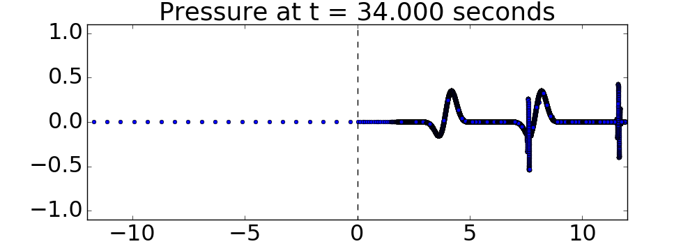
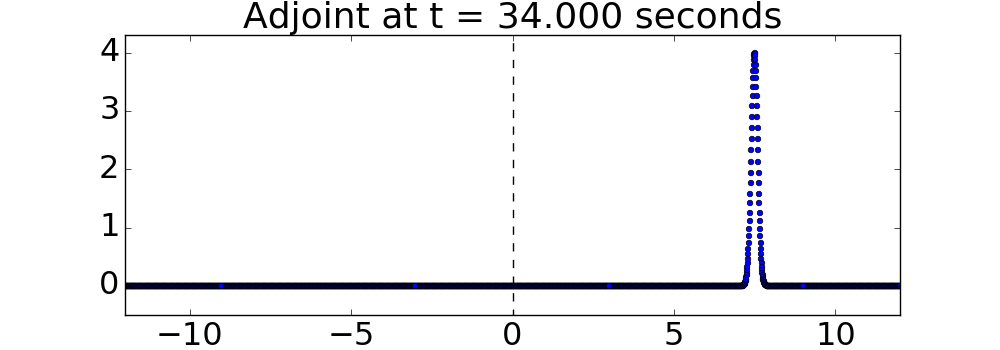
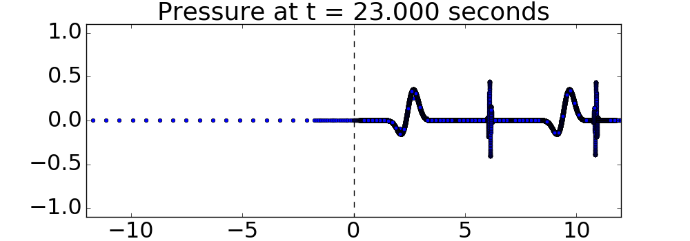
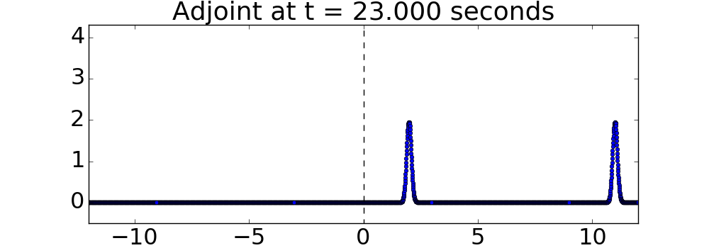
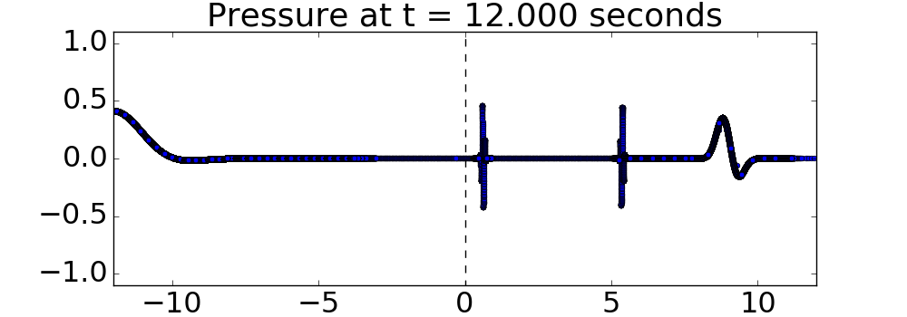
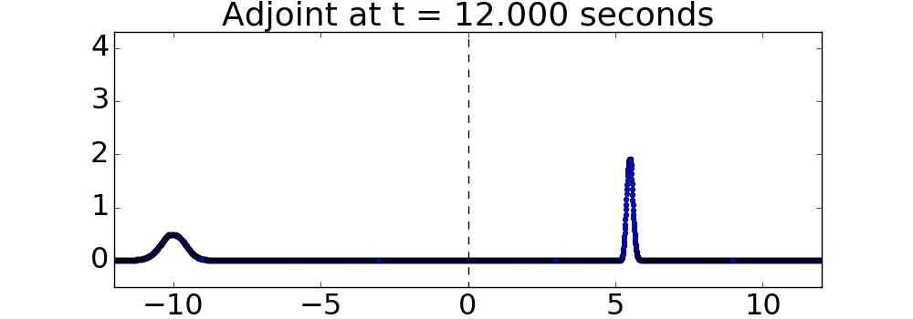
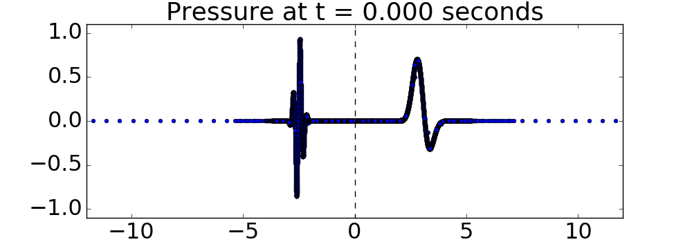
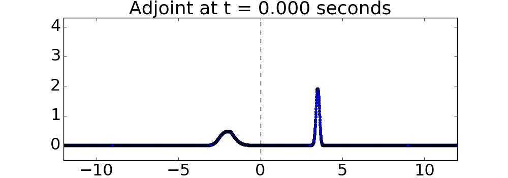
Figure 1. Two wave packets in the forward problem (on the left, with initial data at $t=0$, in the bottom plot) and a Gaussian hump in the adjoint problem (on the right, with “initial” data at $t=34$, in the top plot), interacting with an interface at $x=0$ (dashed line). There is a change of sound speed at the interface, but the impedance is constant throughout the domain. The solutions are plotted as points, whose density varies due to AMR in the left plots.

As the “initial” data for this problem we set $\hat{q}(x,t_{f})=\varphi(x)$. As time progresses backwards, the Gaussian hump splits into equal left-going and right-going waves which interact with the walls and the interface giving reflected waves off of the walls and transmitted waves through the interface. fig:ex1_timeseries shows the AMRClaw results for the pressure of both the forward and adjoint solutions at four different times. Each data point represents the pressure (the $y$ axis) at the center of a grid point in space (the $x$ axis). The density of data points in $x$ is indicative of the resolution of the level of refinement in that location. For instance, in the top plot on the left side of fig:ex1_timeseries, the widely spaced data points on the left side of the domain indicate that the region is covered by a very coarse grid while the tightly spaced data points on the right side of the domain indicate that the region is covered by a very fine grid. Both the forward and adjoint problems are run using $t_{f}=34$, so the forward problem is run from $t=0$ to $t=34$ and the adjoint problem is run from $t=34$ to $t=0$.

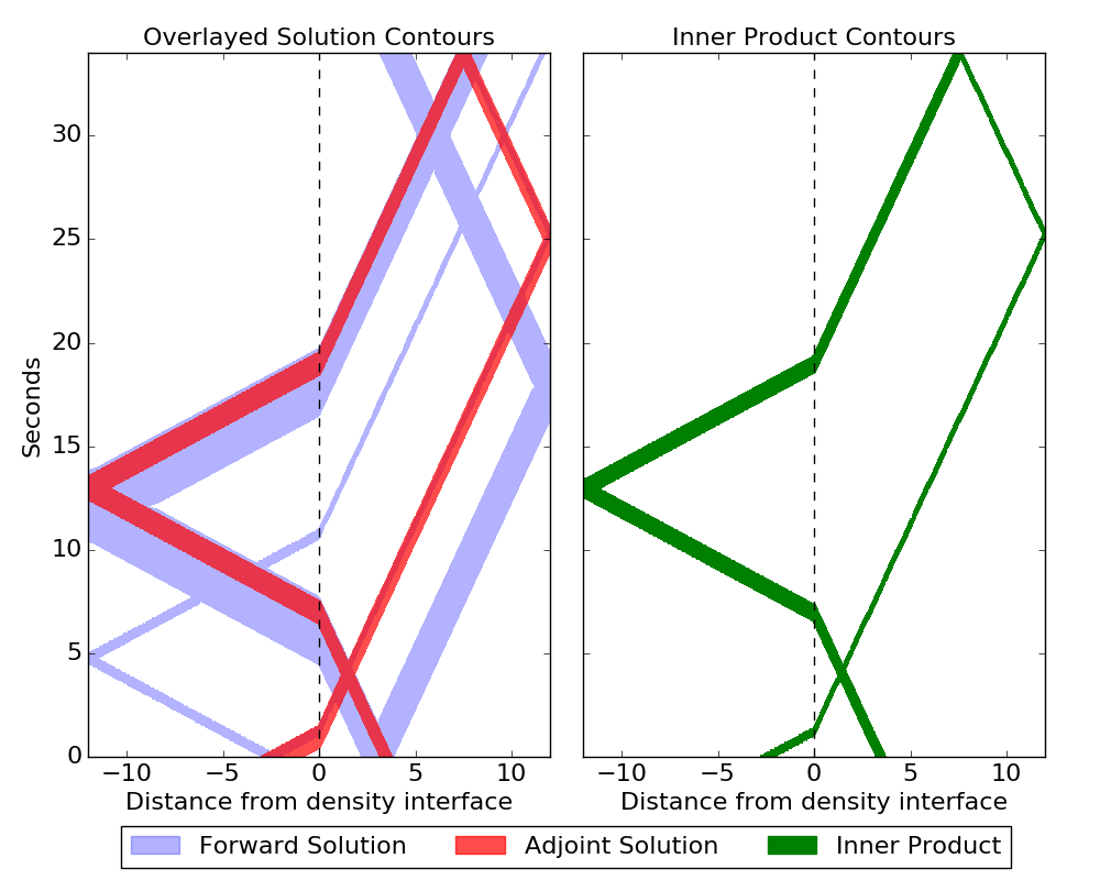
Figure 2. Space-time plots showing the forward and adjoint solutions from Example 1 overlaid in the left plot. Colored regions are where the magnitude of the first component of $q(x,t)$ or $\hat{q}(x,t)$ is above some threshold. The plot on the right shows regions where $|\hat{q}^{T}(x,t)q(x,t)|$ is above some tolerance, indicating where the forward problem should be refined if we are using adjoint-magnitude flagging. The time axis is the same for both plots.

To better visualize how the waves are moving through the domain, it is helpful to look at the data in the $x$-$t$ plane as shown in fig:ex1_norms. For fig:ex1_norms, the horizontal axis is the position, $x$, and the vertical axis is time. The left plot shows in blue the locations where $1-$norm of $q(x,t)$ is greater than or equal to $10^{-2}$ and in red the locations where the $1-$norm of $\hat{q}(x,t)$ is greater than or equal to $10^{-2}$. The right plot shows in green the locations where the inner product $\hat{q}^{T}(x,t)q(x,t)$ is greater than or equal to $10^{-2}$. This indicates which portions of the wave in the forward problem will actually reach our point of interest, and are exactly the regions that will be refined when using the adjoint-magnitude flagging method.

6.2. Example 2: Variable Impedance in One Dimension

As a slightly more complex example, let $t_{0}=0$, $t_{f}=52$, $a=-12$, $b=12$,

$$\rho(x)=\left\{\begin{array}[]{lr}1&\hskip 21.68121pt\textnormal{if }x<0,\\ 2&\textnormal{if }x>0,\end{array}\right.\qquad\text{and}\qquad K(x)=\left\{\begin{array}[]{lr}4&\hskip 21.68121pt\textnormal{if }x<0,\\ 1&\textnormal{if }x>0,\end{array}\right.$$

so that

$$c(x)=\left\{\begin{array}[]{lr}2&\hskip 21.68121pt\textnormal{if }x<0\\ 0.5&\textnormal{if }x>0\end{array}\right.\qquad\text{and}\qquad Z(x)=\left\{\begin{array}[]{lr}4&\hskip 21.68121pt\textnormal{if }x<0,\\ 0.5&\textnormal{if }x>0.\end{array}\right.$$

In this case there is a jump in impedance at $x=0$, which will result in there being both transmitted and reflected waves at the interface. As initial data for $q(x,t)$ we take two wave packets in pressure one on each side of the interface, and zero velocity. The wave packets in pressure are the same as in example 1, and given by eq:1d_qic. As time progresses, the wave packets split into equal left-going and right-going waves which interact with the walls and the interface giving reflected and transmitted waves. In contrast to example 1, many more waves arise in the solution as time evolves due to the generation of new waves at each reflection.

For this example we suppose that we are interested in the accurate estimation of the pressure around $x_{p}=4.5$ at $t=52$, chosen so that several waves in the forward problem must be resolved to accurately capture the solution (while many other waves do not need to be resolved; see fig:ex2_norms). As “initial” data for the adjoint problem, $\hat{q}(x,t_{f})=\varphi(x)$, we can use the same functional eq:phi_1d as in Example 1, with this value of $x_{p}$, and with $\alpha$, and $\hat{\beta}$ defined as in the previous example. As time progresses backwards in the adjoint solution, the hump splits into equal left-going and right-going waves that interact with the walls and the interface giving both reflected and transmitted waves. Both the forward and adjoint problems are run using $t_{f}=52$, so the forward problem is run from $t=0$ to $t=52$ and the adjoint problem is run from $t=52$ to $t=0$.

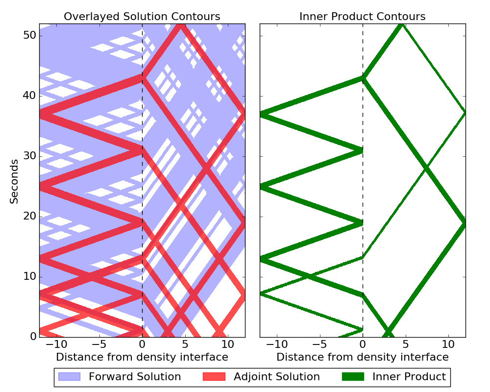
Figure 3. Space-time plots showing the forward and adjoint solutions from Example 2 overlaid in the left plot. Colored regions are where the magnitude of the first component of $q(x,t)$ or $\hat{q}(x,t)$ is above some threshold. The plot on the right shows regions where $|\hat{q}^{T}(x,t)q(x,t)|$ is above some tolerance, indicating where the forward problem should be refined if we are using adjoint-magnitude flagging. The time axis is the same for both plots.

We will again visualize how the waves are moving through the domain by looking at the data in the $x$-$t$ plane as shown in fig:ex2_norms. For fig:ex2_norms, the horizontal axis is the position, $x$, and the vertical axis is time. The left plot shows in blue the locations where $1-$norm of $q(x,t)$ is greater than or equal to $10^{-5}$ and in red the locations where the $1-$norm of $\hat{q}(x,t)$ is greater than or equal to $10^{-3}$. The right plot shows in green the locations where the inner product $\hat{q}^{T}(x,t)q(x,t)$ is greater than or equal to $10^{-3}$. This indicates which portions of the wave in the forward problem will actually reach our point of interest, and are exactly the regions that will be refined when using the adjoint-magnitude flagging method.

To better visualize the impact these different flagging methods have on the final solution, fig:ex2_finalsol_diff shows the final solution when using difference flagging and when using adjoint-magnitude flagging to achieve the same level of accuracy for our functional $J$. Similarly, fig:ex2_finalsol_err shows the final solution when using error flagging and when using adjoint-error flagging to achieve the same level of accuracy in $J$. Note that the adjoint flagging methods have only focused on accurately capturing the waves at the location of interest, whereas the difference and error flagging techniques have captured all of the waves in the domain.

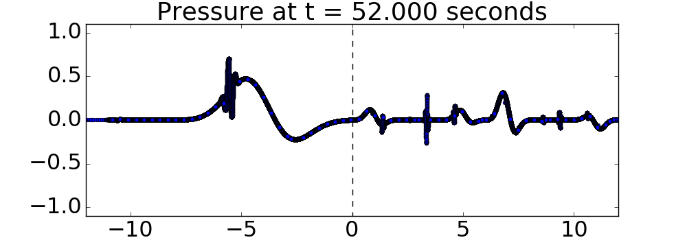
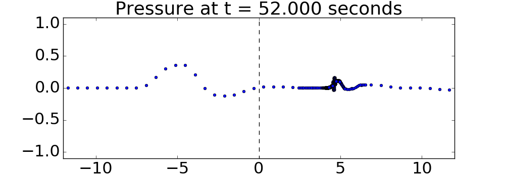
Figure 4. The final solution computed in example 2 when using two different refinement strategies. On the left: using difference-flagging. On the right: using adjoint-magnitude flagging, with a functional $J$ chosen to resolve only the waves that affect the solution near $x_{p}=4.5$ at this time.

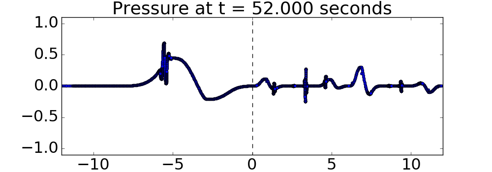
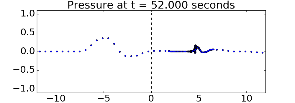
Figure 5. The final solution computed in example 2 when using two different refinement strategies. On the left: using error-flagging. On the right: using adjoint-error flagging, with a functional $J$ chosen to resolve only the waves that affect the solution near $x_{p}=4.5$ at this time.

As an aid to visualizing how the different methods capture the solution at the region of interest, fig:ex2_compare shows the solution for the four different flagging methods for a zoomed-in area around the region of interest. Difference-flagging is shown in blue, error-flagging is shown in red, adjoint-magnitude is flagging shown in green, and adjoint-error flagging is shown in black. Note that although all four solutions (from the four different flagging methods) are show, they are almost impossible to distinguish from one another in the figure. In this figure, only the solution on refinement levels 4 and 5 is shown. Note that the area of the domain that is resolved to refinement levels 4 and 5 is smaller for the adjoint-flagging methods than for their non-adjoint flagging counterparts, as expected.

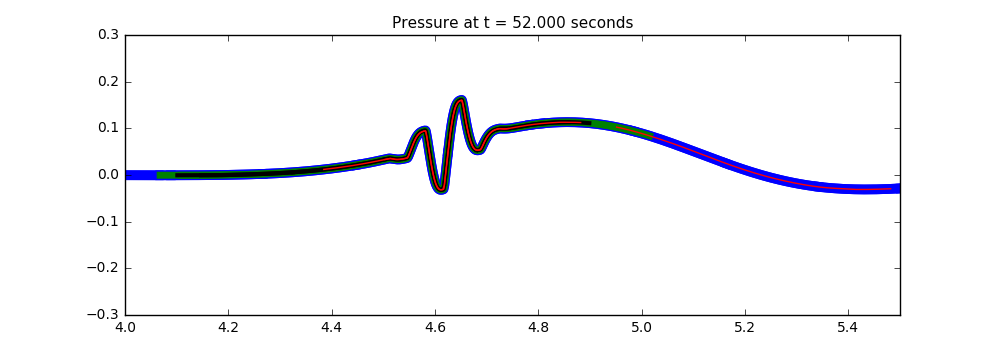
Figure 6. The final solution computed in example 2 for all four refinement strategies, in a zoomed in region of the domain. Difference-flagging shown in blue, error-flagging shown in red, adjoint-magnitude flagging shown in green, and adjoint-error flagging shown in black. Note that the lines are so overlapped that they are almost impossible to tell apart.

6.3. Computational Performance

Recall that we are considering four different flagging methodologies: difference-flagging, error-flagging, adjoint-magnitude flagging, and adjoint-error flagging. To compare the results from these methods we will take into account

• the placement of AMR patches throughout the domain,

• the amount of CPU time required,

• the number of cell updates required, and

• the accuracy of the computed solution

for each flagging method.

Let us begin by considering the placement of AMR levels throughout the domain. Since the adjoint-flagging methods take into account only the portions of the wave that will impact the region of interest during our time range of interest we expect that using adjoint-flagging will result in less of the domain being covered by fine resolution grids — where we are making the assumption that some of the waves will not ultimately have an effect on our region of interest.

In both of the examples we have presented this is in fact the case. Consider the contour plots shown in fig:ex1_norms and fig:ex2_norms. If we are using difference-flagging then anywhere the forward solution is large (all of the areas in blue) would be flagged. In contrast, if we are using adjoint-magnitude flagging all of the areas where the inner product $\hat{q}^{T}(x,t)q(x,t)$ is large (all of the areas in green) would be flagged. Therefore, more of the domain would be flagged when using difference-flagging, resulting in more of the domain being covered by finer levels of refinement. For both of these one-dimensional examples a total of five levels of refinement are used for the forward problem, starting with $40$ cells on the coarsest level and with a refinement ratio of $6$ from each level to the next. So, the finest level in the forward problem corresponds to a fine grid with 51,840 cells. Where these finer levels of refinement are placed, of course, varies based on the flagging method being used. The adjoint problem was solved on a relatively coarse grid with $3000$ cells, and no adaptive mesh refinement.

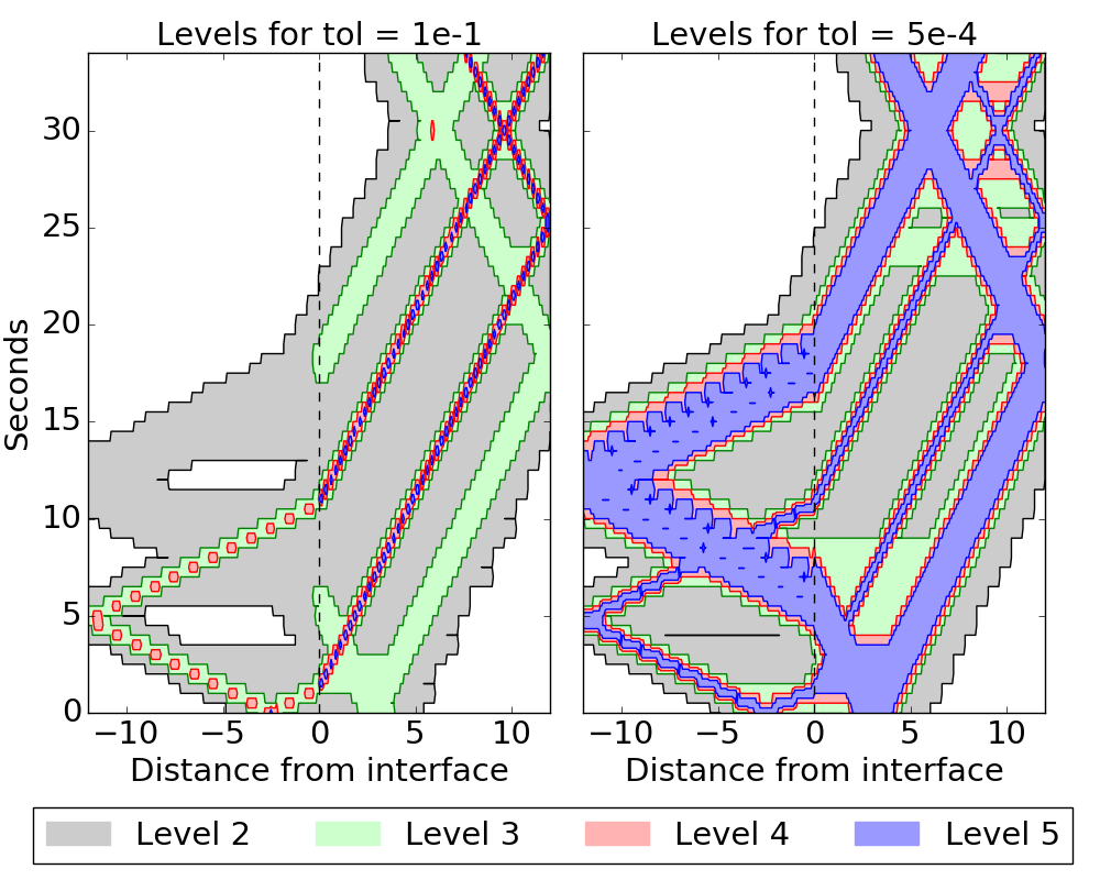
(a) Levels generated by using difference-flagging.

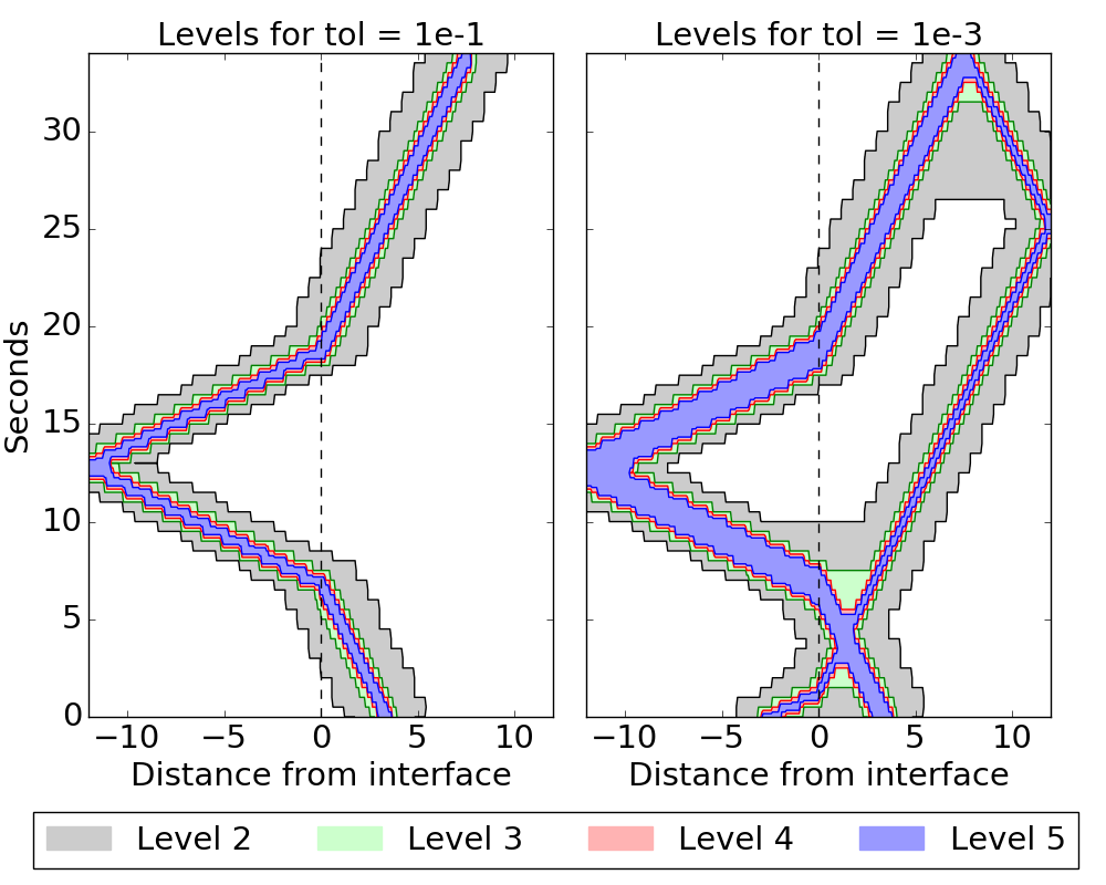
(b) Levels generated by using adjoint-magnitude flagging.

Figure 7. Levels used for the difference-flagging and adjoint-magnitude flagging methods for example 1. Tolerances used for the two difference-flagging runs shown are $10^{-1}$ and $5\times 10^{-4}$. Tolerances used for the two adjoint-magnitude flagging runs shown are $10^{-1}$ and $10^{-3}$. A larger level number means greater resolution: so level 5 for example has a finer resolution than level 4. Recall that level 1 covers the entire domain, and is therefore not shown.

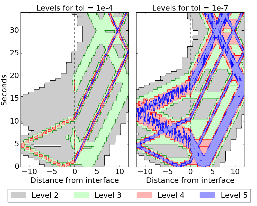
(a) Levels generated by using error-flagging.

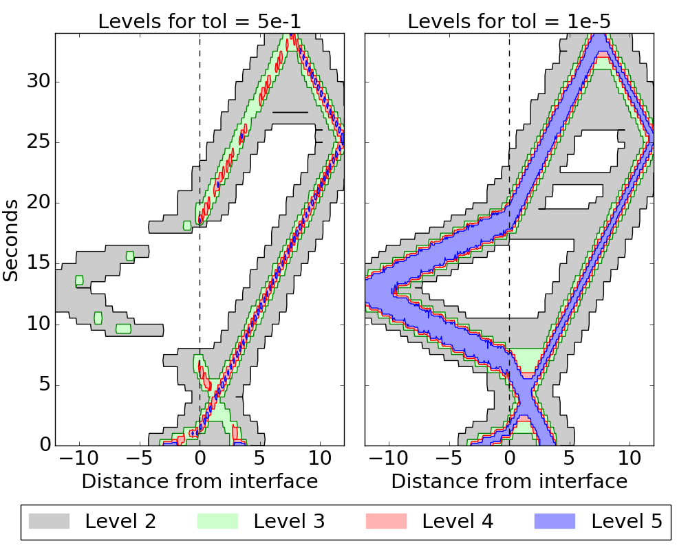
(b) Levels generated by using adjoint-error flagging.

Figure 8. Levels used for the error-flagging and adjoint-error flagging methods for example 1. Tolerances used for the two error-flagging runs shown are $10^{-4}$ and $10^{-7}$. Tolerances used for the two adjoint-error flagging runs shown are $5\times 10^{-1}$ and $10^{-5}$. Recall that level 1 covers the entire domain, and is therefore not shown.

fig:ex1_mag_levels shows the levels of refinement for difference-flagging (on the left) and adjoint-magnitude flagging (on the right) for two different tolerances in example 1. The larger tolerance used for both of these flagging methods is $10^{-1}$ which yields a final error in the functional of interest of about $10^{-2}$ for both methods. The smaller tolerance used for difference flagging is $5\times 10^{-4}$ and for adjoint-magnitude flagging is $10^{-3}$, both of which yield an error of about $10^{-6}$ in the functional of interest. Note that these two flagging methods both consider the value of the pressure in the cell when determining whether or not the cell should be flagged — difference-flagging flags the cell based on the relationship between the pressure in the current cell and the pressure in the adjacent cells, and adjoint-magnitude flagging flags the cell based on the value of the inner product between $q(x,t)$ and $\hat{q}(x,t)$ in the cell. As expected, when the adjoint problem is taken into account the result is a smaller region of the domain begin refined to achieve a comparable level of error.

Similarly, fig:ex1_error_levels shows the levels of refinement for error-flagging (on the left) and adjoint-error flagging (on the right) for two different tolerances in example 1. The larger tolerance used for error-flagging is $10^{-4}$ and for adjoint-error flagging is $5\times 10^{-1}$, both of which yield a final error in the functional of interest of about $10^{-2}$. The smaller tolerance used for error-flagging is $10^{-7}$ and for adjoint-error flagging is $10^{-5}$, both of which yield an error of about $10^{-6}$ in the functional of interest. These two flagging methods consider the estimated error in the solution in each cell when determining whether or not the cell should be flagged. However, the adjoint-error flagging method takes the additional step of considering the inner product of this error estimate with the adjoint solution. Again, when the adjoint problem is taken into account the result is a smaller region of the domain being refined to achieve a comparable final error.

The tolerances shown were selected so that these figures would allow for easy comparison between the four methods. All of the larger tolerances chosen yield an error of about $10^{-2}$ in our functional of interest for each of the methods, and all of the smaller tolerances chosen yield an error of about $10^{-6}$ in our functional of interest. Therefore, it is appropriate to compare the extent of the refined regions present in these figures. Note that even though the same accuracy is achieved, the placement of regions of greater refinement varies between these four methods.

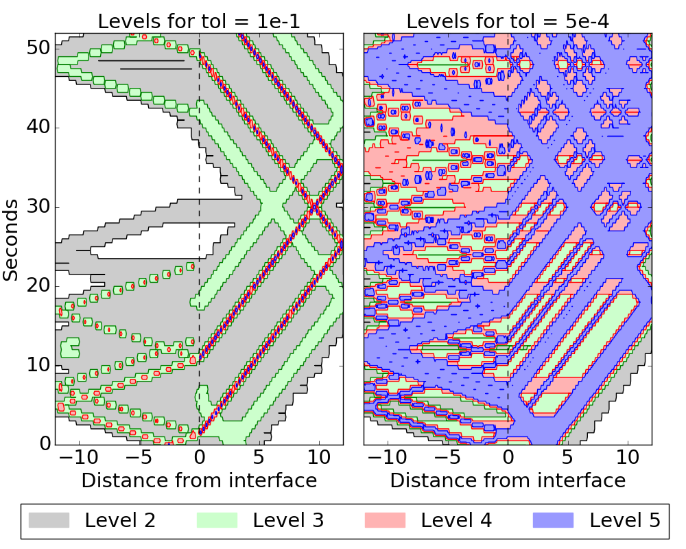
(a) Levels generated by using difference-flagging for example 2.

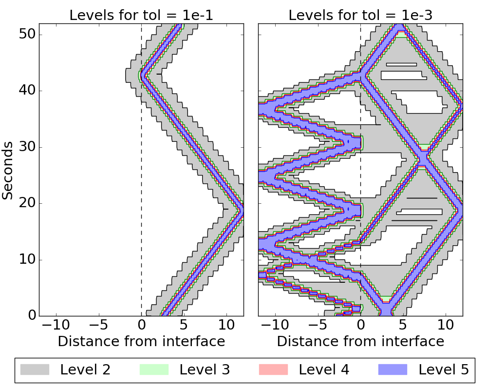
(b) Levels generated by using adjoint-magnitude flagging for example 2.

Figure 9. Levels used for the difference-flagging and adjoint-magnitude flagging methods for example 2. Tolerances used for the two difference-flagging runs shown are $10^{-1}$ and $5\times 10^{-4}$. Tolerances used for the two adjoint-magnitude flagging runs shown are $10^{-1}$ and $10^{-3}$. Recall that level 1 covers the entire domain, and is therefore not shown.

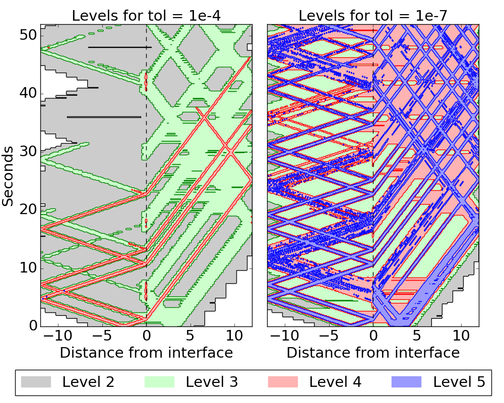
(a) Levels generated by using error-flagging for example 2.

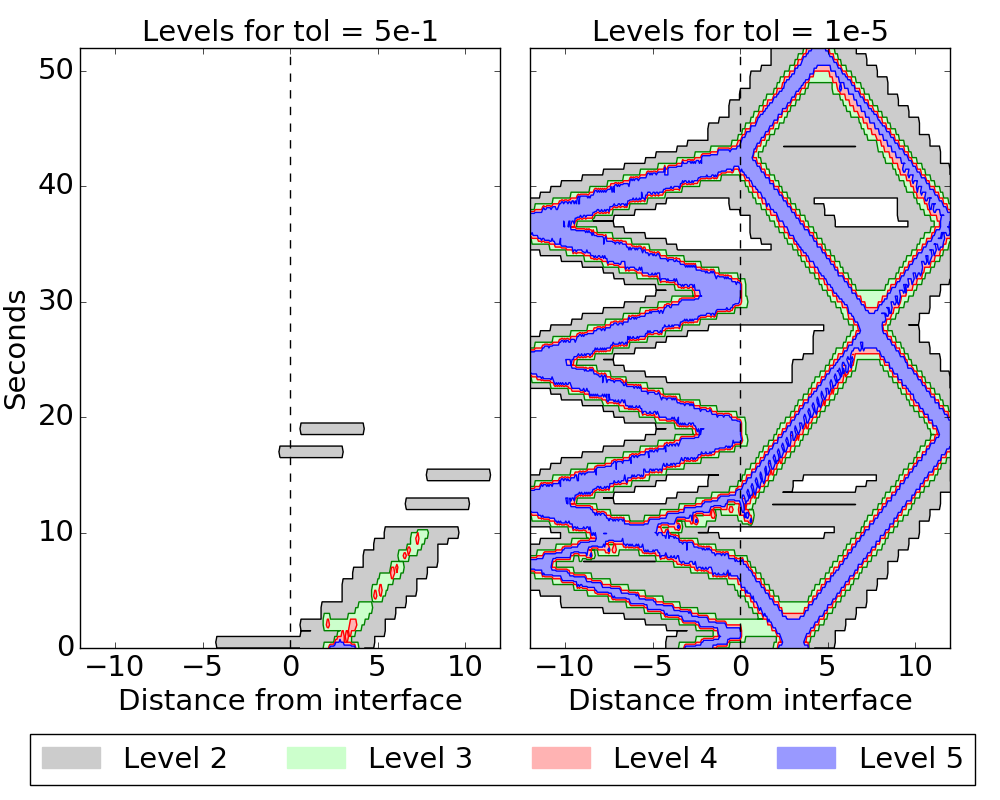
(b) Levels generated by using adjoint-error flagging for example 2.

Figure 10. Levels used for the error-flagging and adjoint-error flagging methods for example 2. Tolerances used for the two error-flagging runs shown are $10^{-4}$ and $10^{-7}$. Tolerances used for the two adjoint-error flagging runs shown are $5\times 10^{-1}$ and $10^{-5}$. Recall that level 1 covers the entire domain, and is therefore not shown.

For example 2, fig:ex2_mag_levels shows the levels of refinement for difference-flagging (on the left) and adjoint-magnitude flagging (on the right) using the same tolerances that were shown for example 1. fig:ex2_error_levels shows the levels of refinement for error-flagging (on the left) and adjoint-error flagging (on the right) for example 2, where we have chosen the same tolerances that were shown for example 1. For this example we again see that when the adjoint problem is taken into account the result is a smaller region of the domain begin refined.

Figure 11. Accuracy for the different flagging methods on example 1. Shown is the error in the functional J for each tolerance value for the various flagging methods.

Also of interest is the amount of work that is required for each of the flagging methods we are considering, and the level of accuracy that resulted from that work. fig:ex1_tolvserror shows the error in our functional of interest given in eq:J for example 1 as the tolerance is varied for the four flagging methods we are considering. Difference-flagging was used with a tolerance of $10^{-12}$ to compute a very fine grid solution to our forward problem for this example. This solution was used to compute a fine grid value of our functional of interest, $J_{\text{fine}}$. The error between the calculated value for $J$ and $J_{\text{fine}}$ is shown.

Note that the magnitude of the error is nearly the same for a given tolerance when using either difference-flagging or adjoint-magnitude flagging although, as we will see, the amount of work required is significantly less when using adjoint-flagging. Also note that the magnitude of the error when using adjoint-error flagging is consistently less than the magnitude of the tolerance being used, as we expected based on sec:adjErrorFlag. This means that adjoint-error flagging allows the user to enforce a certain level of accuracy on the final functional of interest by selecting a tolerance of the desired order. This capability has not existed in Clawpack previous to this work. Recall that the tolerance set by the user is being used to evaluate whether or not some given quantity is above that set tolerance. However, the quantity that is being evaluated is different for each of the flagging methods we are considering. Therefore, other than noting the general trends of each line in this figure, one cannot reach conclusions on relative merits by comparing one line with the others in this plot.

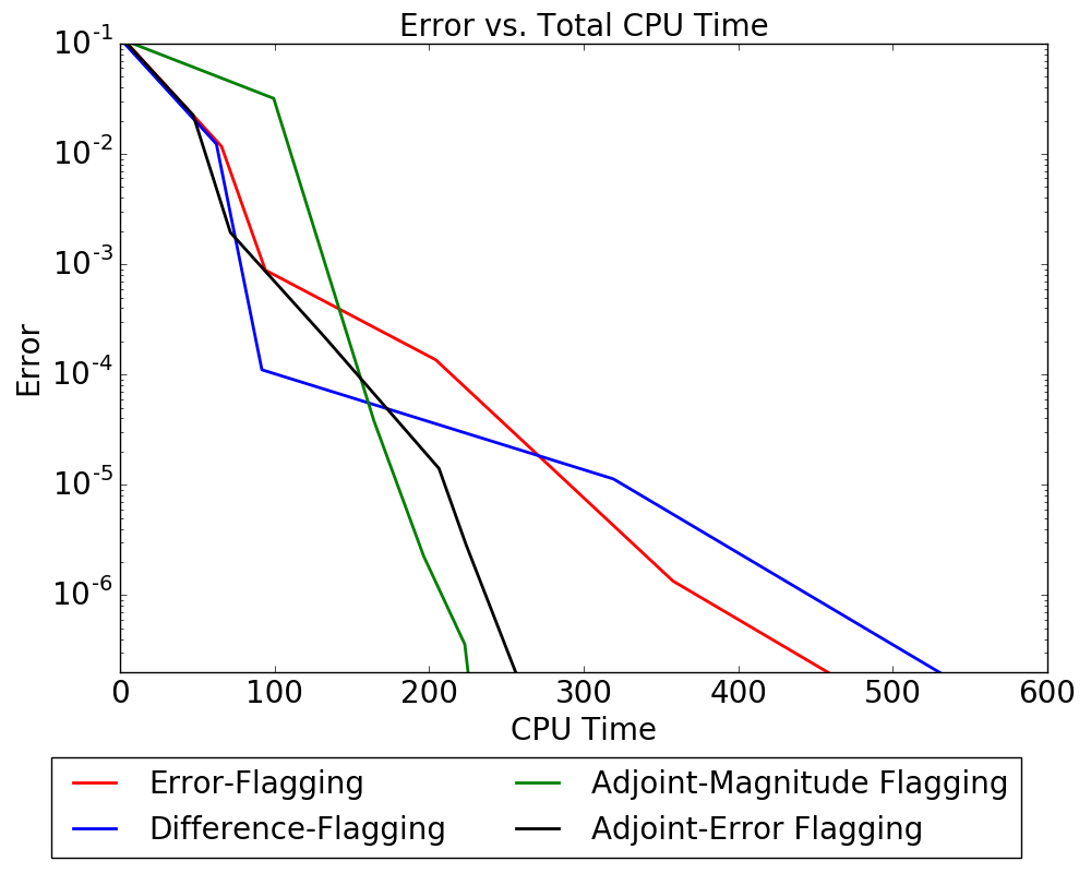
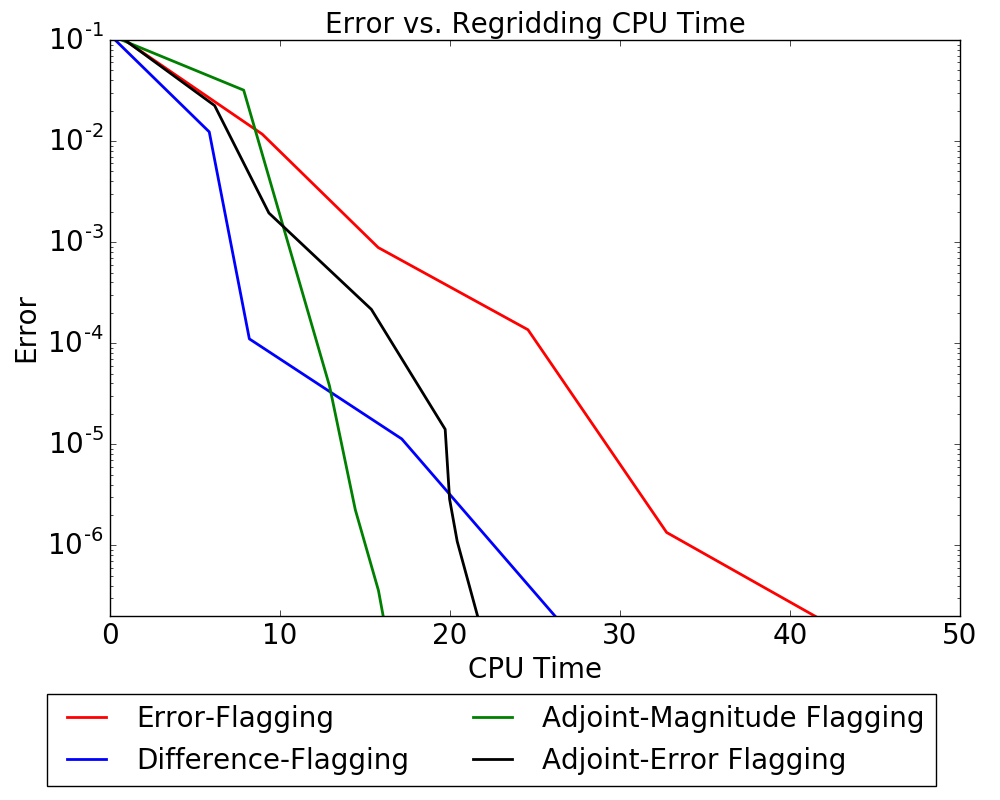
Figure 12. Performance measures for the different flagging methods on example 1. On the left: the total CPU time (in seconds) required vs. the accuracy achieved. On the right: the regridding CPU time (in seconds) required vs. the accuracy achieved. CPU times were found by averaging the CPU time over fifteen runs.

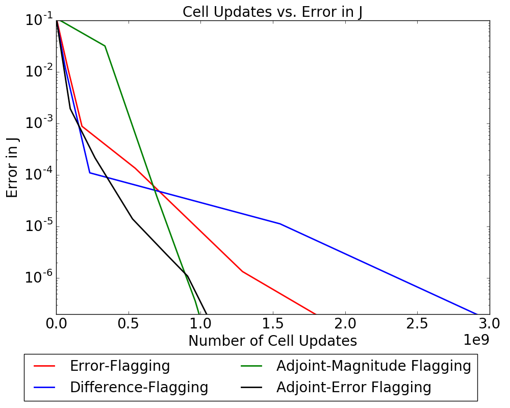
Figure 13. Number of cell updates calculated vs. the accuracy achieved for the four different flagging methods begin considered. Note that the number of cell updates axis is multiplied by $1$e$9$.

We are better able to compare the methods to one another if we consider the amount of computational time that is required to achieve a certain level of accuracy with each flagging method. The above examples were run on a quad-core laptop, and the OpenMP option of AMRClaw was enabled, which allowed all four cores to be utilized. fig:ex1_accuracy shows two measures of the amount of CPU time that was required for each method vs. the accuracy achieved. On the left, we have shown the total amount of CPU time used by the computation. This includes stepping the solution forward in time by updating cell values, regridding at appropriate time intervals, outputting the results, and other various overhead requirements. For each flagging method and tolerance this example was run fifteen times, and the average of the CPU times for those runs was used in this plot. Note that while the adjoint-error and adjoint-difference flagging have higher CPU time requirements for lower accuracy, these two methods quickly show their strength by maintaining a low CPU time requirement while increasing the accuracy of the solution. In contrast, the CPU time requirements for difference-flagging and error-flagging quickly increase when increased accuracy is required. Also remember that the adjoint-flagging methods do have the additional time requirement of solving the adjoint problem, which is not shown in these figures. For this example, solving the adjoint required about 10 seconds of CPU time, which is small compared to the time spent on the forward problem. This CPU time was found by taking the average time required over ten simulations.

The right of fig:ex1_accuracy shows the amount of CPU time spent on the regridding process vs. the accuracy of the functional $J$. Note that this is really where the differences between the four methods lie: the adjoint-flagging methods goal is to reduce the number of cells that are flagged while maintaining the accuracy of the solution. While we have seen from the left side of fig:ex1_accuracy that this has certainly been successful in reducing the overall time required for computing the solution, we might expect that the time spent in the actual regridding process might be longer for the adjoint-flagging methods. This is due to the fact that adjoint-flagging requires various extra steps when determining whether or not to flag a cell (recall, for example, that we need to calculate the inner product between the adjoint and either the forward solution or the estimated error in the forward solution). However, as we can see from this figure, the amount of time spent in the regridding process is not significantly greater for the adjoint-flagging methods. In fact, for higher levels of accuracy the adjoint-flagging methods required less time for the regridding process than their non-adjoint counterparts because there are fewer fine grids.

Another advantage of the adjoint-flagging methods is the fact that they have less memory requirements than the alternative flagging methods. As we have already stated, since the adjoint method allows us to safely ignore regions of the domain, there are fewer fine grids as observed from the fact that many fewer cell updates were required. fig:ex1_cellsvserror shows the number of cell updates required vs. the accuracy achieved for each of the flagging methods being considered. Note that the number of cell updates is significantly less for the adjoint-flagging methods than for their non-adjoint counterparts. This reduces the memory requirements for the computation. For this relatively small example memory usage when utilizing the non-adjoint flagging method did not become an issue, but it can quickly become a constraint for larger computations (in particular for three dimensional problems).

7. Two-Dimensional Variable Coefficient Acoustics

In two dimensions the variable coefficient linear acoustics equations are

(30) $$\begin{split}p_{t}(x,y,t)+K(x,y)\left(u_{x}(x,y,t)+v(x,y,t)_{y}\right)&=0,\\ \rho(x,y)u_{t}(x,y,t)+{p_{x}(x,y,t)}&=0,\\ \rho(x,y)v_{t}(x,y,t)+{p_{y}(x,y,t)}&=0,\end{split}$$

in the domain $x\in[a,b],~{}y\in[\alpha,\beta],~{}t>t_{0}$. Setting

$$A(x,y)=\left[\begin{matrix}0&K(x,y)&0\\ 1/\rho(x,y)&0&0\\ 0&0&0\end{matrix}\right],\hskip 7.22743ptB(x,y)=\left[\begin{matrix}0&0&K(x,y)\\ 0&0&0\\ 1/\rho(x,y)&0&0\end{matrix}\right],\hskip 7.22743ptq(x,y,t)=\left[\begin{matrix}p(x,y,t)\\ u(x,y,t)\\ v(x,y,t)\end{matrix}\right],$$

gives us the equation $q_{t}(x,y,t)+A(x,y)q_{x}(x,y,t)+B(x,y)q_{y}(x,y,t)=0$.

As an example, consider $t_{0}=0$, $t_{f}=21$, $a=-8$, $b=8$, $\alpha=-1$, $\beta=11$,

$$\rho(x,y)\equiv 1,\qquad\text{and}\qquad K(x,y)=\left\{\begin{array}[]{lr}4&\hskip 21.68121pt\textnormal{if }x<0,\\ 1&\textnormal{if }x>0,\end{array}\right.$$

so that

$$c(x,y)=\left\{\begin{array}[]{ll}2&\hskip 21.68121pt\textnormal{if }x<0,\\ 1&\hskip 21.68121pt\textnormal{if }x>0,\end{array}\right.\qquad\text{and}\qquad Z(x,y)=\left\{\begin{array}[]{ll}2&\hskip 21.68121pt\textnormal{if }x<0,\\ 1&\hskip 21.68121pt\textnormal{if }x>0.\end{array}\right.$$

We use wall boundary conditions on the top and both sides,

(31) $$u(a,y,t)=0,\hskip 7.22743ptu(b,y,t)=0 t\geq 0,$$

(32) $$v(x,\beta,t)=0 t\geq 0,$$

and extrapolation boundary conditions on the bottom at $y=-1$. The impedance jump at $x=0$ will result in reflected and transmitted waves emanating from this interface. Also, we will have reflected waves from the walls along both sides and the top of our domain.

As initial data for $q(x,y,t)$ we take a smooth radially symmetric hump in pressure, and a zero velocity in both $x$ and $y$ directions. The initial hump in pressure is given by

(35) $$p(x,y,0)=\left\{\begin{array}[]{lr}3+\cos\left(\pi\left(r-0.5\right)/w\right)&\hskip 21.68121pt\textnormal{if }\left|r-0.3\right|\leq w,\\ 0&\textnormal{otherwise.}\end{array}\right.$$

with $w=0.15$ and $r=\sqrt{\left(x-0.5\right)^{2}+\left(y-1\right)^{2}}$. As time progresses, this hump in pressure will radiate outward symmetrically.

We will consider two different examples, one where there are just a few waves that intersect at our region of interest during our time range of interest, and a second where a larger number of waves contribute to our region and time range of interest.

7.1. Example 3: Capturing a few intersecting waves

Suppose that we are interested in the accurate estimation of the pressure in the area defined by a rectangle centered about $(x,y)=(1.0,5.5)$ at the final time $t_{f}=21$. The small rectangle in fig:2d_adjoint_ex3 and later figures shows this region of interest. Setting

$$J=\int_{0.68}^{1.32}\int_{5.26}^{5.74}p(x,y,t_{f})dy\,dx,$$

the problem then requires that

(36) $$\varphi(x,y)=\left[\begin{matrix}I(x,y)\\ 0\\ 0\end{matrix}\right],$$

where

(39) $$I(x,y)=\left\{\begin{array}[]{ll}1&\hskip 21.68121pt\textnormal{if }0.68\leq x\leq 1.32\textnormal{ and }5.26\leq y\leq 5.74,\\ 0&\hskip 21.68121pt\textnormal{otherwise.}\end{array}\right.$$

Define

$$\hat{q}(x,y,t_{f})=\left[\begin{matrix}\hat{p}(x,y,t_{f})\\ \hat{u}(x,y,t_{f})\\ \hat{v}(x,y,t_{f})\end{matrix}\right]=\varphi(x,y),$$

and note that for any time $t_{0}<t_{f}$ we have

$$\int_{t_{0}}^{t_{f}}\int_{a}^{b}\int_{\alpha}^{\beta}\hat{q}^{T}\left(q_{t}+A(x,y)q_{x}+B(x,y)q_{y}\right)dy\,dx\,dt=0.$$

Integrating by parts yields the equation

$$\left.\int_{a}^{b}\int_{\alpha}^{\beta}\hat{q}^{T}q\,dy\,dx\right|^{t_{f}}_{t_{0}} +\left.\int_{t_{0}}^{t_{f}}\int_{\alpha}^{\beta}\hat{q}^{T}A(x,y)q\,dy\,dt\right|^{b}_{a}+\left.\int_{t_{0}}^{t_{f}}\int_{a}^{b}\hat{q}^{T}B(x,y)q\,dx\,dt\right|^{\beta}_{\alpha}$$

(40) $$- \int_{t_{0}}^{t_{f}}\int_{a}^{b}\int_{\alpha}^{\beta}q^{T}\left(\hat{q}_{t}+\left(A^{T}(x,y)\hat{q}\right)_{x}+\left(B^{T}(x,y)\hat{q}\right)_{y}\right)dy\,dx\,dt=0.$$

Note that if we can define an adjoint problem such that all but the first term in this equation vanishes then we are left with

$$\int_{a}^{b}\int_{\alpha}^{\beta}\hat{q}^{T}(x,y,t_{f})q(x,y,t_{f})dy\,dx=\int_{a}^{b}\int_{\alpha}^{\beta}\hat{q}^{T}(x,y,t_{0})q(x,y,t_{0})dy\,dx,$$

which is the expression that allows us to use the inner product of the adjoint and forward problems at each time step to determine what regions will influence the point of interest at the final time. We can accomplish this by defining the adjoint problem

(41) $$\hat{q}_{t}+\left(A^{T}(x,y)\hat{q}\right)_{x}+\left(B^{T}(x,y)\hat{q}\right)_{y}=0 x\in[a,b],y\in[\alpha,\beta],\hskip 7.22743ptt_{f}\geq t\geq t_{0}$$

with the same boundary conditions as the forward problem.

As the initial data for the adjoint $\hat{q}(x,y,t_{f})=\varphi(x,y)$ we have a square pulse in pressure, which was described in eq:phi_2d_ex3 and eq:delta_2d_ex3. As time progresses backwards, waves radiate outward and reflect off the walls as well as transmitting and reflecting off of the interface at $x=0$. The adjoint problem was solved on a $200\times 200$ grid without mesh refinement, and several snapshots of the solution are shown in fig:2d_adjoint_ex3. The location of interest is outlined with a black box in the plots.

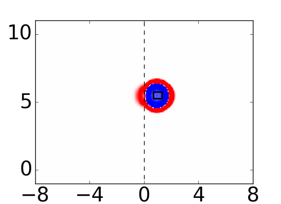
(a) $t_{f}-$ 1 second

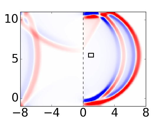
(b) $t_{f}-$ 6 seconds

(c) $t_{f}-$ 15 seconds

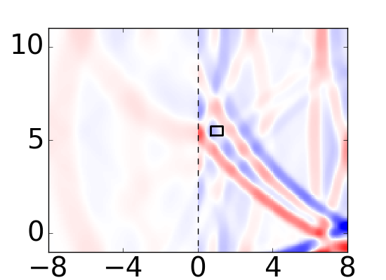
(d) $t_{f}-$ 18.5 seconds

Figure 14. Computed results for two-dimensional acoustics adjoint problem for example 3. Times shown are the number of seconds before the final time, since the “initial” conditions are given at the final time. The small rectangle in this and later figures shows the region of interest defined by the functional $J$, and is the region where $I(x,y)=1$. The color scale goes from blue to red, and ranges between $-0.005$ and $0.005$.

Although we have focused on the functional $J$, and are considering the accuracy and error in our estimates of this functional, in actuality we are typically interested in the accurate estimation of the pressure in the forward solution at a particular spatial and temporal area. The selection of the initial data for the adjoint plays a role in determining the functional $J$, and dictates the relationship between the solution of the forward problem and our functional of interest. Therefore, the initial data we select for the adjoint problem is undoubtedly significant. For this example we have selected initial conditions for the adjoint problem such that our functional $J$ is simply the integral of the forward solution over our region of interest. For the one-dimensional examples shown earlier, a Gaussian initial condition for the adjoint was used. An exploration of how these initial conditions affect the accuracy of the forward solution is not conducted in this work, but is an interesting area for future work.

t = 2.5 seconds

t = 6 seconds

t = 15 seconds

t = 21 seconds

Fine Grid

Solution

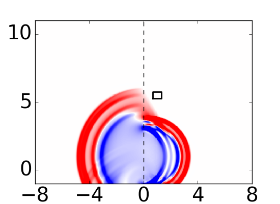
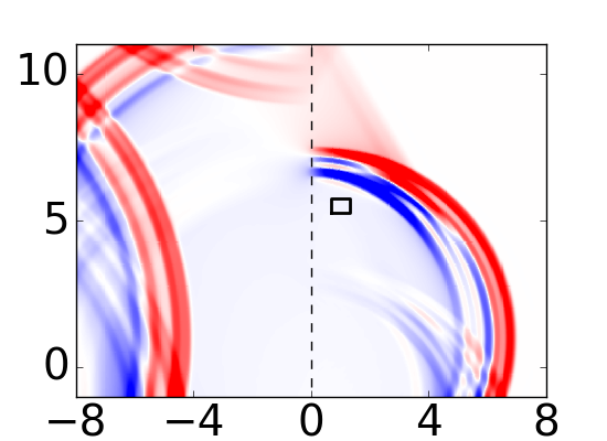
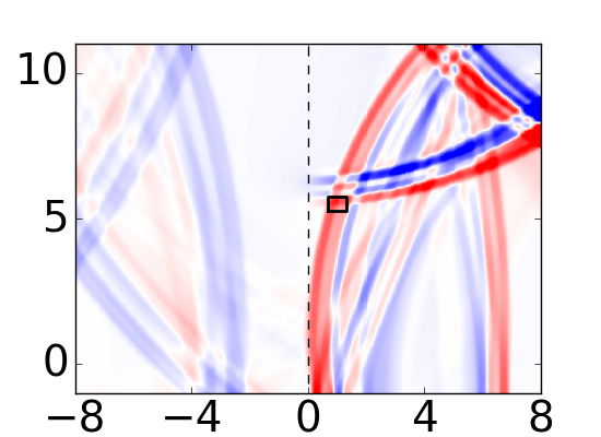
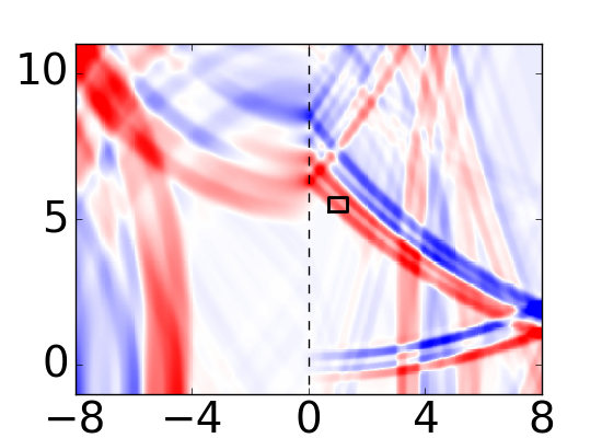
Difference-Flagging

Grids

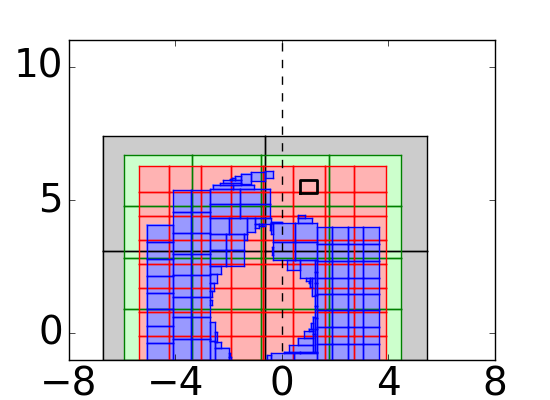
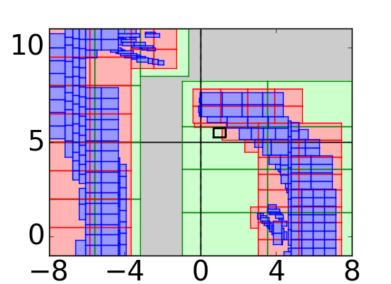
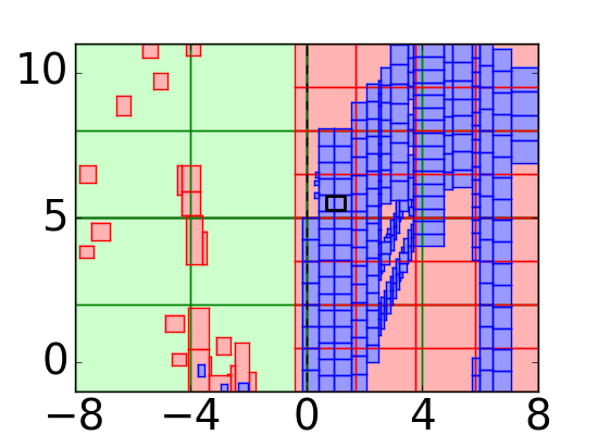
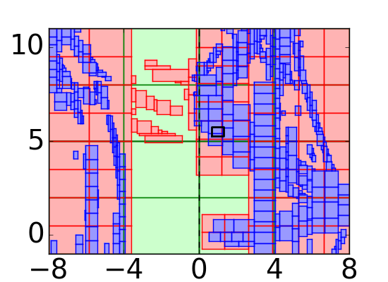
Error-Flagging

Grids

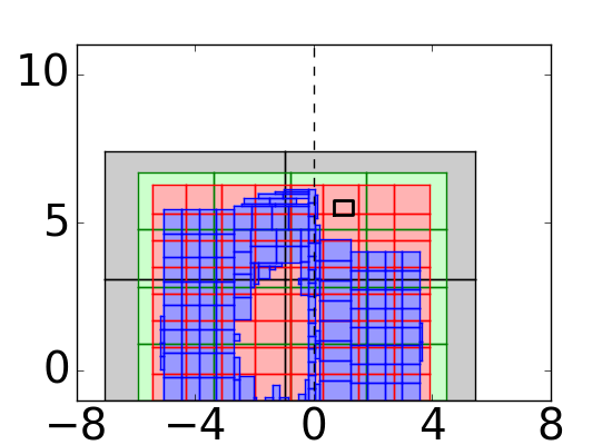
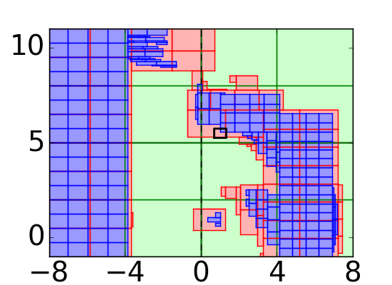
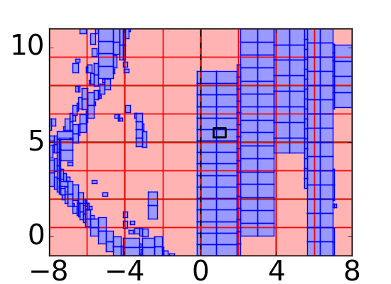
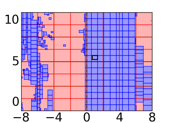
Adjoint-Magnitude

Flagging Grids

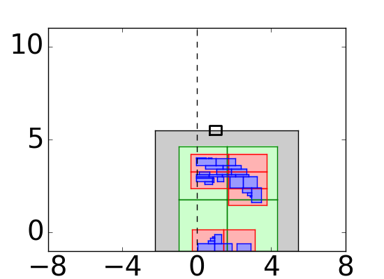
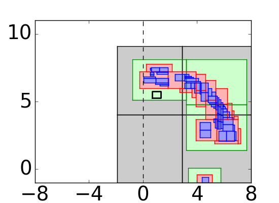
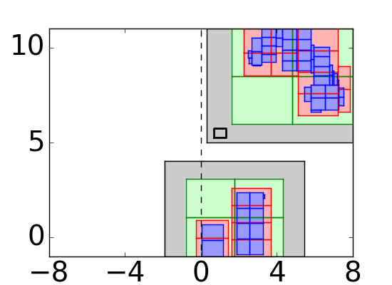
Adjoint-Error

Flagging Grids

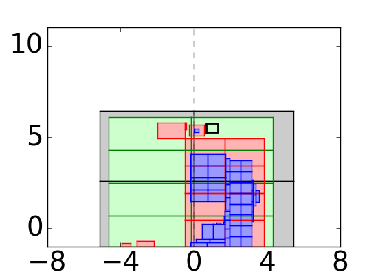
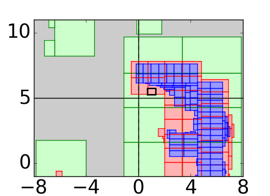
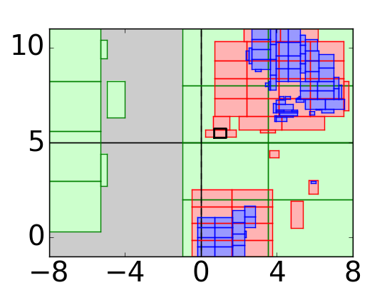
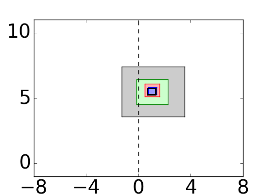
Figure 15. Plots for the two dimensional forward problem for example 3. The top row shows the fine grid solution, and the bottom four rows each show the grids for the different refinement levels being used for this problem when it is solved using one of the four flagging methods being presented. The color scale for the fine grid solution figures goes from blue to red, and ranges between $-0.3$ and $0.3$. For all of the refinement level plots the coarsest refinement level is shown in white, and the second, third, fourth and fifth levels of refinement are shown in grey, green, red, and blue, respectively.

fig:2d_plot_ex3 compares the refinement levels used by each of the four different flagging methods on the forward problem for this example. Difference-flagging was used with a tolerance of $10^{-12}$ to compute a fine grid solution to our forward problem. The top row of the figure shows this fine grid solution, for the sake of reference. Each of the following rows shows the refinement patches (colored by level) being used in the simulation, from which we can quickly note that the adjoint-flagging methods have smaller regions of refinement than the other two flagging methods. The location of interest is outlined with a black box on all of the plots. For each of these flagging methods five levels of refinement are allowed for the forward problem, where the coarsest level is a $50\times 50$ grid and a refinement ratio of 2 in both $x$ and $y$ is used from each grid to the next. So, the finest level in the forward problem corresponds to a fine grid of $1600\times 1600$ cells. For all of the refinement level plots the coarsest refinement level is shown in white, and the second, third, fourth and fifth levels of refinement are shown in grey, green, red, and blue, respectively. Where these finer levels of refinement are placed, of course, varies based on the flagging method being used. The adjoint problem was solved on a relatively coarse grid of $200\times 200$ cells, and no adaptive mesh refinement. (As a side note, this problem was also computed with the adjoint problem solved on a coarse grid of $50\times 50$ cells with nearly the same final results. The $200\times 200$ cells adjoint was used for the figures shown here, since it provided clearer plots for fig:2d_adjoint_ex3). The tolerance used for the difference-flagging plots shown was $3\times 10^{-2}$, for the adjoint-magnitude flagging plots the tolerance used was $3\times 10^{-4}$, for the error-flagging plots the tolerance used was $6\times 10^{-5}$, and for the adjoint-error flagging plots the tolerance used was $3\times 10^{-3}$. These tolerances were chosen because they all resulted in an error of about $5\times 10^{-4}$ in our functional $J$. Therefore, it is appropriate to compare the placement of the refined patches in the plots shown for all four flagging methods.

Note that, as in the one-dimensional examples, the new adjoint-based approaches allow refinement to occur only around the waves that eventually coalesce on the location of interest, with a region very close to the rectangle defined by the functional $J$ being refined at the final time $t_{f}=21$. By contrast, the original difference-flagging and error-flagging approaches lead to refinement of many waves and portions of the domain that have no benefit in terms of determining the functional $J$ accurately.

7.2. Example 4: Capturing many intersecting waves

How much of the domain must be refined with the adjoint approach depends on the specification of $J$. In this final example we simply move the location of interest to a place where more waves are converging at $t_{f}$ in order to illustrate that the adjoint approach will adapt to this situation. Suppose that we are now interested in the accurate estimation of the pressure in the area defined by a rectangle centered about $(x,y)=(3.5,0.5)$, and define

$$J=\int_{3.18}^{3.82}\int_{0.26}^{0.74}p(x,y,t_{f})dy\,dx.$$

For this example, the definition of the adjoint problem is the same as in example 3 except for the “initial data”, for which we now take $\hat{q}(x,y,t_{f})=\varphi(x,y)$ where $\varphi$ is as in eq:phi_2d_ex3 with $I(x,y)$ now defined by

(44) $$I(x,y)=\left\{\begin{array}[]{ll}1&\hskip 21.68121pt\textnormal{if }3.18\leq x\leq 3.82\textnormal{ and }0.26\leq y\leq 0.74,\\ 0&\hskip 21.68121pt\textnormal{otherwise.}\end{array}\right.$$

As time progresses backwards, waves radiate outward and reflect off the walls as well as transmitting and reflecting off of the interface at $x=0$.

t = 2.5 seconds

t = 6 seconds

t = 15 seconds

t = 21 seconds

Fine Grid

Solution

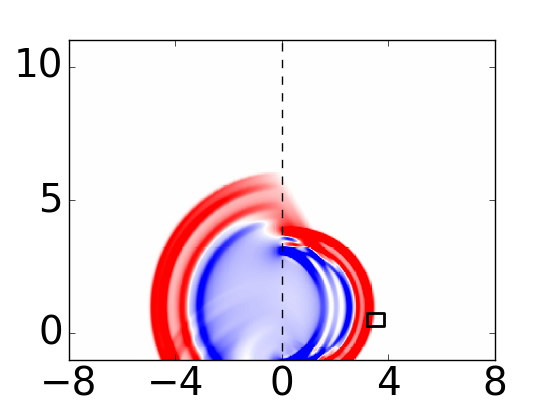
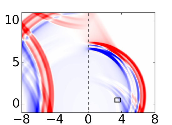
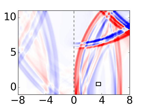
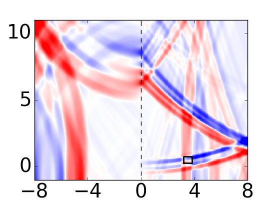
Adjoint-Magnitude

Flagging Grids

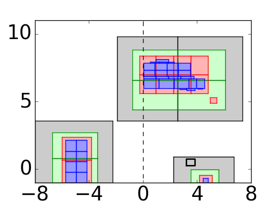
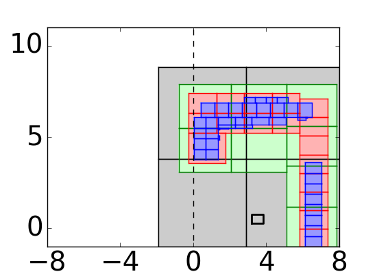
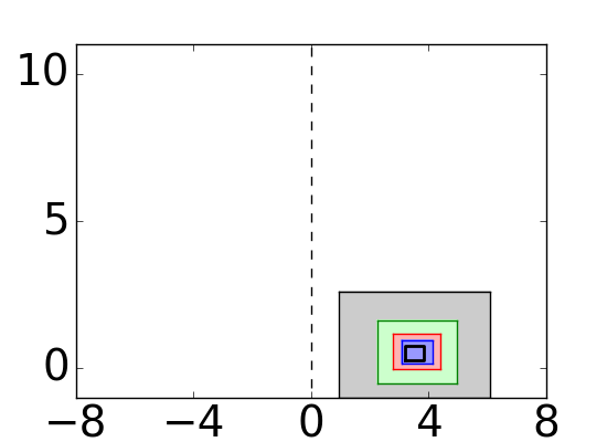
Adjoint-Error

Flagging Grids

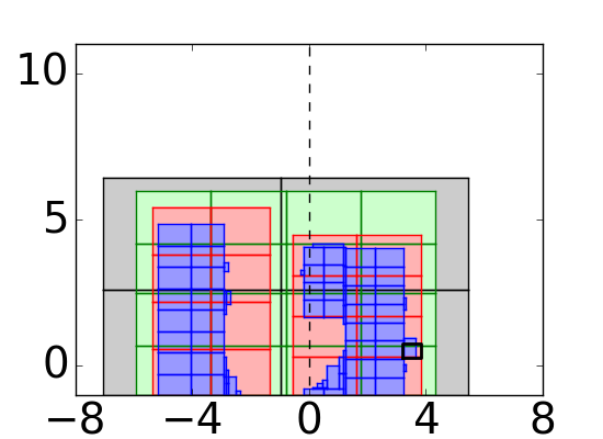
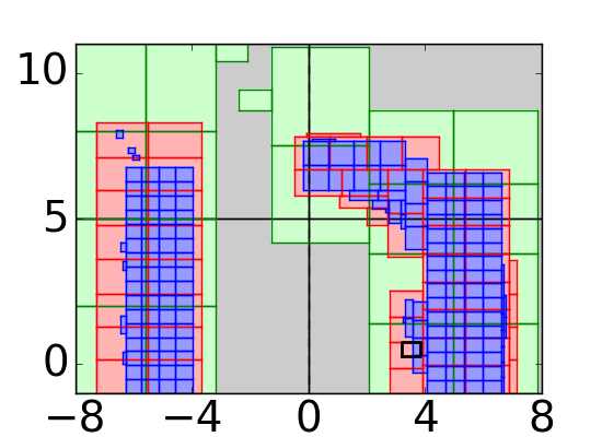
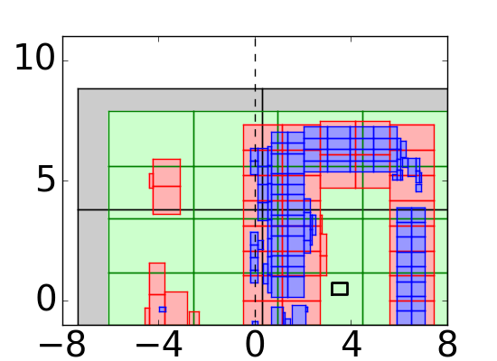
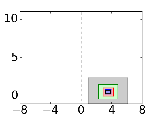
Figure 16. Plots for the two dimensional forward problem for example 4. The top row shows the fine grid solution, and the bottom two rows each show the grids for the different refinement levels being used for this problem when it is solved using one of the two adjoint-flagging methods. The color scale for the fine grid solution figures goes from blue to red, and ranges between $-0.3$ and $0.3$. For all of the refinement level plots the coarsest refinement level is shown in white, and the second, third, fourth and fifth levels of refinement are shown in grey, green, red, and blue, respectively.

fig:2d_plot compares the refinement levels used by each of the two adjoint-flagging methods on the forward problem for this example. The top row of the figure shows the fine grid solution once again, for the sake of reference and to show the new location of interest. The new location of interest is outlined with a black box on all of the plots. As with fig:2d_plot_ex3, each of the following rows shows the refinement patches (colored by level) being used in the simulation. For each of these flagging methods five levels of refinement are allowed for the forward problem, where the coarsest level is a $50\times 50$ grid and a refinement ratio of 2 in both $x$ and $y$ is used from each grid to the next. So, as with example 3, the finest level in the forward problem corresponds to a fine grid of $1600\times 1600$ cells. For all of the refinement level plots the coarsest refinement level is shown in white, and the second, third, fourth and fifth levels of refinement are shown in grey, green, red, and blue, respectively. Where these finer levels of refinement are placed, of course, varies based on the flagging method being used. The adjoint problem was again solved on a relatively coarse grid of $200\times 200$ cells without adaptive mesh refinement.

The tolerance used for these plots are the same as the ones shown for example 3. Note that for the same tolerance the fine grid, difference flagging, and error flagging solutions are the same as in example 3, except for the placement of the gauge. Since none of these computations depended on the adjoint method, changing the area of interest (which changes the initial conditions for the adjoint problem) does not affect the computation. Since they would be the same as fig:2d_plot_ex3, the figures for difference-flagging and error-flagging grids are not repeated in fig:2d_plot.

7.3. Computational Performance

The advantage of using the adjoint method can be seen in the amount of work that is required for each of the flagging methods we are considering, and the level of accuracy that results from that work. fig:2d_tolvserror shows the error in our functional of interest for the two-dimensional acoustics example 3 as the tolerance is varied for the four flagging methods we are considering. Our fine grid solution was used to calculate a fine grid value of our functional of interest, $J_{\text{fine}}$. The error between the calculated value of $J$, from the various tolerances used for each of the flagging methods, and $J_{\text{fine}}$ is shown.

Of particular interest, note that the magnitude of the error when using adjoint-error flagging is once again consistently less than the magnitude of the tolerance being used, as we expected based on sec:adjErrorFlag. This means that, as with example 1, adjoint-error flagging allows the user to enforce a certain level of accuracy on the final functional of interest by selecting a tolerance of the desired order. Recall that the tolerance set by the user is being used to evaluate whether or not some given quantity is above that set tolerance. However, the quantity that is being evaluated is different for each of the flagging methods we are considering. Therefore, other than noting the general trends in this figure, not much benefit comes from comparing each of the lines corresponding to a flagging method to the others in this plot.

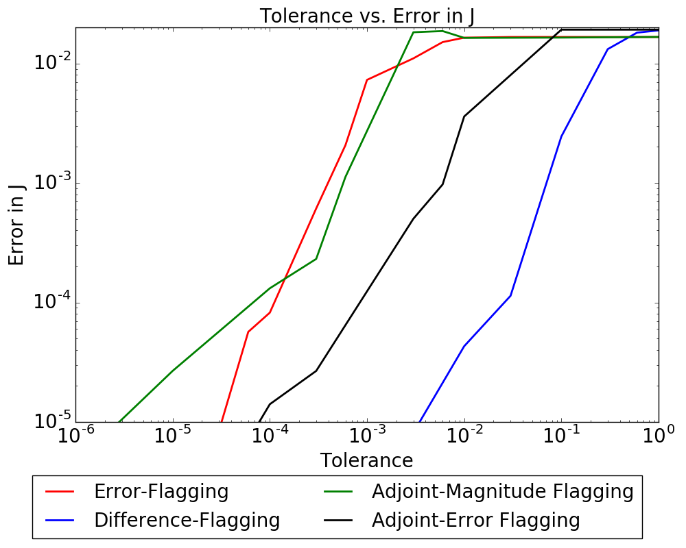
Figure 17. Accuracy for the different flagging methods on the two-dimensional acoustics example 3. Shown is the error in the functional $J$ for each tolerance value for the various flagging methods.

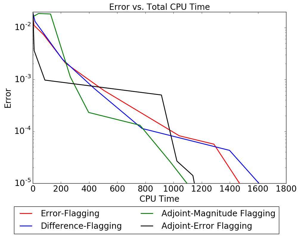
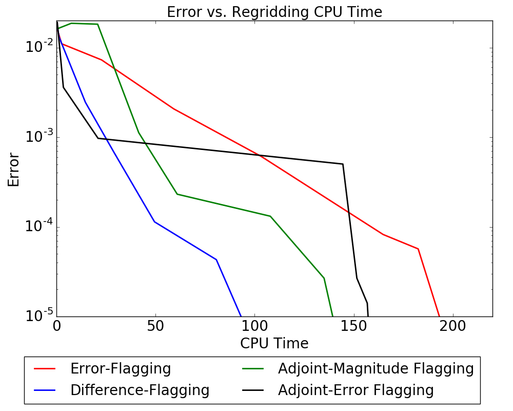
Figure 18. Performance measures for the different flagging methods on the two-dimensional acoustics example 3. On the left: the total CPU time (in seconds) required vs. the accuracy achieved. On the right: the regridding CPU time (in seconds) required vs. the accuracy achieved. CPU times were found by averaging the CPU time over ten runs.

We are better able to compare the methods to one another if we consider the amount of computational time that is required to achieve a certain level of accuracy with each flagging method. As with the one-dimensional examples, both of the two-dimensional examples was run on a quad-core laptop, and the OpenMP option of AMRClaw was enabled which allowed all four cores to be utilized. fig:2d_accuracy shows two measures of the amount of CPU time that was required for each method vs. the accuracy achieved for example 3. On the left, we have shown the total amount of CPU time used by the computation. This includes stepping the solution forward in time by updating cell values, regridding at appropriate time intervals, outputting the results, and other various overhead requirements. For each flagging method and tolerance this example was run ten times, and the average of the CPU times for those runs was used to generate this plot. As with the one-dimensional example, while the adjoint-magnitude and adjoint-error flagging methods have a higher CPU time requirement for lower accuracy, these methods quickly showed their strength by maintaining a low CPU time requirement while increasing the accuracy of the solution. In contrast, the CPU time requirements for difference-flagging and error-flagging are larger than their adjoint-flagging counterparts when increased accuracy is required. Note that the adjoint-flagging methods do have the additional time requirement of solving the adjoint problem, which is not shown in these figures. For this example, solving the adjoint required about 37 seconds of CPU time, which is once again small compared to the time spent on the forward problem. As before, this CPU time was found by taking the average time required over ten simulations.

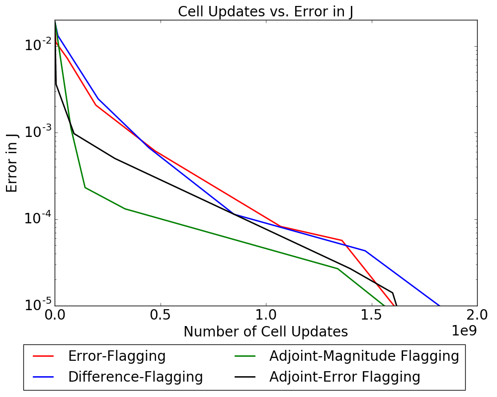
Figure 19. Number of cell updates calculated vs. the accuracy achieved for the four different flagging methods begin considered for example 3. Note that the number of cell updates axis is multiplied by $1$e$9$.

The right of fig:2d_accuracy shows the amount of CPU time spent on the regridding process vs. the accuracy of the functional $J$. Note that this is really where the differences between the four methods lie: the adjoint-flagging methods goal is to reduce the number of cells that are flagged while maintaining the accuracy of the solution. While we have seen from the left side of fig:2d_accuracy that this has certainly been successful for adjoint-flagging in reducing the overall time required for computing the solution, we might expect that the time spent in the actual regridding process might be longer for the adjoint-flagging methods. However the amount of time spent in the regridding process is not significantly greater for the adjoint-flagging methods.

As with the one-dimensional example, here we see that the adjoint-flagging methods have less memory requirements than the alternative flagging methods. fig:ex3_cellsvserror shows the number of cell updates required vs. the accuracy achieved for each of the flagging methods being considered. While the results are not as drastic as what we saw for example 1, note that the number of cell updates for example 3 is consistently less for the adjoint-flagging methods than for their non-adjoint counterparts, since there are fewer fine grids throughout the domain. This reduces the memory requirements for the computation. This example is also relatively small, and memory usage when utilizing the non-adjoint flagging method did not become an issue. However, in larger simulations (for instance, ocean-wide problems when considering tsunami modeling) memory constraints can become a significant consideration. It can also become a significant consideration in three dimensional problems.

8. Conclusions and Future Work

In this paper we have presented a method for using the adjoint equation to guide adaptive mesh refinement when solving hyperbolic systems of equations, as well as describing the implementation of this method into the AMRClaw software package. The adjoint method was used to identify the waves which should be refined to ensure an accurate estimation of the solution at the final time, provided we were interested in some target region (for example, the location of a pressure gauge).

Two different methods for identifying cells that should be refined were presented: adjoint-magnitude flagging and adjoint-error flagging. These two methods were compared to the two main flagging methods currently available in AMRCLAW: difference-flagging and error-flagging. Accuracy and timing results for various examples were presented, and for each example the results from using all four of these flagging methods were compared.

It was shown that using adjoint-flagging provides confidence that the appropriate waves have been refined to accurately capture the solution at the target location, without unnecessary refinemement in other regions. For the examples considered, both adjoint-magnitude flagging and adjoint-error flagging had the advantage of requiring less computational time than their non-adjoint counterparts to achieve the same level of accuracy in the final solution. Also, the adjoint-flagging methods required fewer cell updates to achieve the same level of accuracy, which signifies a smaller memory requirement.

The code for all the examples presented in this work is available online at (Davis, 2018a). This code can be easily modified to solve other linear variable coefficient acoustics problems. This repository also contains other examples illustrating how adjoint-flagging can be used with AMRClaw and GeoClaw. These adjoint-flagging procedures are now being incorporated into the Clawpack software and should be available in future releases for general use.

In this work we have focused on examples involving the linear acoustics equations. However, the adjoint method is not limited to working on only these equations. For examples using the adjoint method to guide adaptive mesh refinement for the shallow water equations in the context of tsunami modeling see (Davis and LeVeque, 2016; Borrero et al., 2015). Using the adjoint method when solving non-linear equations requires that the equations be linearized. In the context of using the shallow water equations for tsunami propagation across the ocean this is fairly straight forward, since they can be linearized about the ocean at rest. An area of future work is studying the use of the adjoint method in the context of other nonlinear hyperbolic equations, where the adjoint equation would be derived by linearizing about a particular forward solution. This would require the development of some kind of automated process to shift between solving the forward problem, linearizing about that forward problem, solving the corresponding adjoint problem, and using that adjoint solution in guiding the adaptive mesh refinement for the forward problem.

We have focused in this work on the accurate calculation of the functional $J$, where the definition for this functional varied based on the target area of interest. However, we are typically concerned with the accurate estimation of the solution to the forward problem rather than the functional $J$. For the examples presented in this work we used various different initial conditions for the adjoint problem, but did not consider the effect this had on the accuracy of the forward solution. Examining the implications of the initial conditions used for the adjoint problem, and their effect on the accuracy of the foward solution, is another area for future work.

Appendix A Riemann solvers used in this work

In this appendix, we present some details regarding the Riemann problems encountered when solving the forward and adjoint equations for variable-coefficient linear acoustics. A Riemann problem is the hyperbolic equation of interest together with initial data that is piecewise constant with a single jump discontinuity, say,

$$q_{0}(x)=\left\{\begin{array}[]{lr}q_{l}&\textnormal{if }x<0\\ q_{r}&\textnormal{if }x>0\end{array}\right.$$

where $q_{l}$ and $q_{r}$ are constant state vectors. For variable-coefficient linear problems, the Riemann problem also assumes that the variable coefficients have a jump discontinuity at $x=0$, e.g., from $\rho_{l}$ to $\rho_{r}$.

For the acoustics equations $q_{t}+A(x)q_{x}=0$ with $A(x)$ given by eq:Aacoustics, it is easy to compute that the eigenvalues are

$$\lambda^{1}=-c(x)\hskip 21.68121pt\textnormal{and}\hskip 21.68121pt\lambda^{2}=c(x)$$

where $c(x)=\sqrt{K(x)/\rho(x)}$ is the speed of sound in material. The eigenvectors for this matrix $A(x)$ are

$$r^{1}=\left[\begin{matrix}-Z(x)\\ 1\end{matrix}\right]\hskip 21.68121pt\textnormal{and}\hskip 21.68121ptr^{2}=\left[\begin{matrix}Z(x)\\ 1\end{matrix}\right],$$

where $Z(x)=\rho(x)c(x)$ is the impedance. Note that any scalar multiple of these vectors would still be an eigenvector of $A(x)$. This particular normalization was chosen for consistency with (LeVeque, 2004), where many more details are given about Riemann solutions and the manner in which these are used as the building block for the high-resolution finite volume methods implemented in Clawpack.

The solution to the Riemann problem for acoustics consists of two waves, a left-going sound wave with speed $-c_{l}$ and a right-going sound wave with speed $c_{r}$. The left-going wave moves into a homogeneous material with impedance $Z_{l}$ and hence the jump in $q$ across this wave is a multiple of the eigenvector $r^{1}_{l}=[-Z_{l},1]^{T}$, while the jump in $q$ across the right-going wave must be a multiple of $r^{1}_{r}=[Z_{r},1]^{T}$. Between these two waves the state $q_{m}$ must be constant across the jump in material properties at $x=0$, or else the resulting stationary jump in $q$ would lead to a delta function singularity in $q_{t}$ according to the PDE. This structure is illustrated in fig:q_waves.

Therefore, we wish to find $q_{m}$ such that

$$q_{m}-q_{l}=\alpha^{1}\left[\begin{matrix}-Z_{l}\\ 1\end{matrix}\right]\equiv\mathcal{W}^{1}_{rl}\hskip 21.68121pt\textnormal{and}\hskip 21.68121ptq_{r}-q_{m}=\alpha^{2}\left[\begin{matrix}Z_{r}\\ 1\end{matrix}\right]\equiv\mathcal{W}^{2}_{rl}$$

for some scalar coefficients $\alpha^{1}$ and $\alpha^{2}$. If we add these two equations together we get

$$q_{r}-q_{l}=\alpha^{1}\left[\begin{matrix}-Z_{l}\\ 1\end{matrix}\right]+\alpha^{2}\left[\begin{matrix}Z_{r}\\ 1\end{matrix}\right].$$

This gives us a linear system of two equations to solve for $\alpha^{1}$ and $\alpha^{2}$. The solution of this gives us the decomposition of the jump in $q$ as the sum of the two acoustic waves,

(45) $$q_{r}-q_{l}=\sum\limits_{p=1}^{2}\alpha^{p}r^{p}\equiv\sum\limits_{p=1}^{2}\mathcal{W}^{p}_{rl}$$

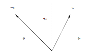
Figure 20. Structure of the solution to the Riemann problem for the forward problem, in the $x-t$ plane. The dashed line depicts the interface between two different cells. Between the waves is a single state $q_{m}$. For the adjoint problem with initial states $\tilde{q}_{l}$ and $\tilde{q}_{r}$ the wave speeds are the same but there will be two intermediate states $\tilde{q}_{ml}$ and $\tilde{q}_{mr}$ to either side of the dashed line. Figure from (LeVeque, 2004).

When solving the Riemann problem for the modified adjoint equation $\tilde{q}_{t}-(A(x)^{T}\tilde{q})_{x}=0$ that is solved forward in time (see eq:1d_adjoint_modified), the eigenvalues of $-A(x)^{T}$ are the same as the eigenvalues of $A(x)$, but the eigenvectors are now

$$\tilde{r}^{1}=\left[\begin{matrix}1\\ Z(x)\end{matrix}\right]\hskip 21.68121pt\textnormal{and}\hskip 21.68121pt\tilde{r}^{2}=\left[\begin{matrix}1\\ -Z(x)\end{matrix}\right].$$

Since the adjoint equation is in conservation form, it is the flux $\tilde{f}(\tilde{q},x)\equiv-A(x)^{T}\tilde{q}$ that must be continuous across $x=0$ in order to avoid a singularity, and so $\tilde{q}$ will generally have have a jump from $\tilde{q}_{ml}$ to $\tilde{q}_{mr}$ across $x=0$, while $\tilde{f}(\tilde{q}_{ml})=\tilde{f}(\tilde{q}_{mr})\equiv\tilde{f}_{m}$.

As before, the jump across each wave is given by an eigenvector of the coefficient matrix from the appropriate material. Therefore, we have that

$$\tilde{f}_{m}-\tilde{f}_{l}=\beta^{1}\left[\begin{matrix}1\\ Z_{l}\end{matrix}\right]\hskip 21.68121pt\textnormal{and}\hskip 21.68121pt\tilde{f}_{r}-\tilde{f}_{m}=\beta^{2}\left[\begin{matrix}1\\ -Z_{r}\end{matrix}\right]$$

for some scalar coefficients $\beta^{1}$ and $\beta^{2}$. If we add these two equations together we get

$$\tilde{f}_{r}-\tilde{f}_{l}=\beta^{1}\left[\begin{matrix}1\\ Z_{l}\end{matrix}\right]+\beta^{2}\left[\begin{matrix}1\\ -Z_{r}\end{matrix}\right].$$

This gives us a linear system of equations to solve for $\beta^{1}$ and $\beta^{2}$. These so-called f-waves can be used directly in the f-wave version of the wave-propagation algorithms used in Clawpack, as discussed further in (Bale et al., 2002), or these can be converted into jumps in $\tilde{q}$ as follows. Since the left-going and right-going waves propagate through constant materials, we have (by the Rankine-Hugoniot jump conditions) that

$$\tilde{q}_{ml}-\tilde{q}_{l}=\frac{\tilde{f}_{m}-\tilde{f}(\tilde{q}_{l})}{\lambda^{1}_{l}}=-\frac{\beta^{1}}{c_{l}}\left[\begin{matrix}1\\ Z_{l}\end{matrix}\right],\qquad\tilde{q}_{r}-\tilde{q}_{ml}=\frac{\tilde{f}(\tilde{q}_{r}))-\tilde{f}_{m}}{\lambda^{2}_{r}}=\frac{\beta^{2}}{c_{r}}\left[\begin{matrix}1\\ Z_{r}\end{matrix}\right],$$

which allows determining the jumps in $\tilde{q}$ across each propagating wave.

More complete details can be found in the references cited above, and in the Clawpack code implementing the examples shown in this paper, all of which can be found in (Davis, 2018a).

References

- (1)
- Bale et al. (2002) D. Bale, R. J. LeVeque, S. Mitran, and J. A. Rossmanith. 2002. A wave-propagation method for conservation laws and balance laws with spatially varying flux functions. SIAM J. Sci. Comput. 24 (2002), 955–978.
- Becker and Rannacher (2001) R. Becker and R. Rannacher. 2001. An optimal control approach to a posteriori error estimation in finite element methods. Acta Numerica 10 (2001), 1–102.
- Berger and Rigoutsos (1991) M. Berger and I. Rigoutsos. 1991. An algorithm for point clustering and grid generation. IEEE T. Syst. Man Cyb. 21, 5 (Sep 1991), 1278–1286.
- Berger and Colella (1989) M. J. Berger and P. Colella. 1989. Local Adaptive Mesh Refinement for Shock Hydrodynamics. J. Comput. Phys. 82 (1989), 64–84.
- Berger et al. (2011) M. J. Berger, D. L. George, R. J. LeVeque, and K. T. Mandli. 2011. The GeoClaw software for depth-averaged flows with adaptive refinement. Adv. Water Res. 34 (2011), 1195–1206. www.clawpack.org/links/papers/awr11
- Berger and LeVeque (1998) M. J. Berger and R. J. LeVeque. 1998. Adaptive Mesh Refinement Using Wave-Propagation Algorithms for Hyperbolic Systems. SIAM J. Numer. Anal. 35, 6 (October 1998), 2298–2316.
- Berger and Oliger (1984) M. J. Berger and J. Oliger. 1984. Adaptive Mesh Refinement for Hyperbolic Partial Differential Equations. J. Comput. Phys. 53 (1984), 484–512.
- Borrero et al. (2015) J. C. Borrero, R. J. LeVeque, D. Greer, S. O’Neill, and B. N. Davis. 2015. Observations and Modelling of Tsunami Currents at the Port of Tauranga, New Zealand. In Australasian Coasts & Ports Conference 2015. Engineers Australia and IPENZ, Auckland, New Zealand, 90–95.
- Clawpack Development Team (2015) Clawpack Development Team. 2015. Clawpack software. http://www.clawpack.org Version 5.3.
- Davis (2018a) B. N. Davis. Accessed 2018a. Adjoint code repository. https://github.com/BrisaDavis/adjoint
- Davis (2018b) B. N. Davis. Accessed 2018b. Riemann code repository. https://github.com/BrisaDavis/riemann/tree/adjoint
- Davis and LeVeque (2016) B. N. Davis and R. J. LeVeque. 2016. Adjoint Methods for Guiding Adaptive Mesh Refinement in Tsunami Modeling. Pure Appl. Geophys. 173 (2016), 4055–4074. https://doi.org/10.1007/s00024-016-1412-y
- Jameson (1988) A. Jameson. 1988. Aerodynamic design via control theory. J. Sci. Comput. 3, 3 (1988), 233–260.
- Kast and Fidkowski (2013) S. M. Kast and K. J. Fidkowski. 2013. Output-based mesh adaptation for high order Navier-Stokes simulations on deformable domains. J. Comput. Phys. 252 (2013), 468–494.
- Kouhi et al. (2015) M. Kouhi, E. Oñate, and D. Mavriplis. 2015. Adjoint-based adaptive finite element method for the compressible Euler equations using finite calculus. Aerospace Science and Technology 46 (2015), 422 – 435. https://doi.org/10.1016/j.ast.2015.08.008
- Lacasta et al. (2018) A. Lacasta, M. Morales-Hernández, Pilar Brufau, and Pilar García-Navarro. 2018. Application of an adjoint-based optimization procedure for the optimal control of internal boundary conditions in the shallow water equations. Journal of Hydraulic Research 56, 1 (2018), 111–123. https://doi.org/10.1080/00221686.2017.1300196 arXiv:https://doi.org/10.1080/00221686.2017.1300196
- Langseth and LeVeque (2000) J. O. Langseth and R. J. LeVeque. 2000. A wave-propagation method for three-dimensional hyperbolic conservation laws. J. Comput. Phys. 165 (2000), 126–166.
- LeVeque (1997) R. J. LeVeque. 1997. Wave Propagation Algorithms for Multidimensional Hyperbolic Systems. J. Comput. Phys. 131, CP965603 (1997), 327–353.
- LeVeque (2004) R. J. LeVeque. 2004. Finite Volume Methods for Hyperbolic Problems. Cambridge University Press, Cambridge, UK.
- LeVeque et al. (2011) R. J. LeVeque, D. L. George, and M. J. Berger. 2011. Tsunami modeling with adaptively refined finite volume methods. Acta Numerica 20 (2011), 211–289.
- Luo and Fidkowski (2011) Y. Luo and K. J. Fidkowski. 2011. Output-based space-time mesh adaptation for unsteady aerodynamics.
- Mandli et al. (2016) K. T. Mandli, A. J. Ahmadia, M. Berger, D. Calhoun, D. L. George, Y. Hadjimichael, D. I. Ketcheson, G. I. Lemoine, and R. J. LeVeque. 2016. Clawpack: building an open source ecosystem for solving hyperbolic PDEs. PeerJ Computer Science 2 (2016), e68. https://doi.org/10.7717/peerj-cs.68
- Mandli and Dawson (2014) K. T. Mandli and C. N. Dawson. 2014. Adaptive mesh refinement for storm surge. Ocean Modelling 75 (March 2014), 36–50. https://doi.org/10.1016/j.ocemod.2014.01.002
- Marburger (2012) J. Marburger. 2012. Adjoint-Based Optimal Control of Time-Dependent Free Boundary Problems. http://arxiv.org/abs/1212.3789
- Nadarajah and Jameson (2000) S. Nadarajah and A. Jameson. 2000. A comparison of the continuous and discrete adjoint approach to automatic aerodynamic optimization. In 38th Aerospace Sciences Meeting and Exhibit. American Institute of Aeronautics and Astronautics, Reno,NV. https://doi.org/10.2514/6.2000-667
- Park (2004) M. A. Park. 2004. Adjoint-Based, Three-Dimensional Error Prediction and Grid Adaptation. AIAA Journal 42 (2004), 1854–1862.
- Pierce and Giles (2000) N. A. Pierce and M. B. Giles. 2000. Adjoint recovery of superconvergent functionals from PDE approximations. SIAM Rev. 42 (2000), 247–264.
- Sanders and Katopodes (2000) B. F. Sanders and N. D. Katopodes. 2000. Adjoint Sensitivity Analysis for Shallow-Water Wave Control. J. Eng. Mech. 126, 9 (2000), 909–919.
- Venditti and Darmofal (2002) D. A. Venditti and D. L. Darmofal. 2002. Grid Adaptation for Functional Outputs: Application to Two-Dimensional Inviscid Flows. J. Comput. Phys. 176, 1 (2002), 40 – 69. https://doi.org/10.1006/jcph.2001.6967
- Venditti and Darmofal (2003) D. A. Venditti and D. L. Darmofal. 2003. Anisotropic grid adaptation for functional outputs: application to two-dimensional viscous flows. J. Comput. Phys. 187, 1 (2003), 22 – 46. https://doi.org/10.1016/S0021-9991(03)00074-3