On The Discovery Of The Seed
In Uniform Attachment Trees

Abstract.

We investigate the size of vertex confidence sets for including part of (or the entirety of) the seed in seeded uniform attachment trees, given knowledge of some of the seed’s properties, and with a prescribed probability of failure. We also study the problem of identifying the leaves of a seed in a seeded uniform attachment tree, given knowledge of the positions of all internal nodes of the seed.

1. Introduction

In the web graph, nodes represent websites, and edges represent links. Its theoretical study requires proper graph models that explain and approximate what is observed in the field—see [5] for an early book on this topic. One particular set of models grows the web graph dynamically, one new website at a time. This leads to the study of random graph dynamics [15, 28]. The main—but still simple—models here are the uniform random recursive tree and the preferential attachment model. Simple generalizations of these tree models in which $k$ instead of one parent are selected at each step lead to graphs. We are concerned in this paper with the estimation of the origin of the tree when one is shown the entire (unrooted) tree. In particular, we consider only uniform attachment trees that are grown started from a fixed tree $S$, called the seed, a problem first studied by Bubeck et al. [8, 9]. Estimating the seed can aid, for example, in the identification of the source of a rumour, an idea, or an epidemic. Finding the source of an epidemic can help to identify the original causes for the spread of the infection, and aid in the development of preventative measures. The area of discovering the origins of the web graph or a social network graph is also called network archeology.

Consider the random tree which begins as some fixed tree $S$ and grows incrementally by adding a new vertex and connecting it to a uniformly random node among all nodes. We think of the starting tree as the seed of the process, and we continue the attachment process for a long time. We ask the following question: How difficult is it to identify the position of the seed in such a process only given the structure of the tree? In general, what aspects of the seed can be identified efficiently?

The growth process, started from a single node, yields the uniform random recursive tree (URRT) or uniform attachment tree (see e.g., [12, 14, 23, 24]). We take the following point of view, following [7]: Given the uniform attachment tree $T$, and a fixed $\varepsilon>0$, our algorithm returns a set $H=H(T,\varepsilon)$ of nodes such that, in the case that $|S|=1$,

$$\operatorname{\mathbf{P}}\{V(S)\subseteq H\}\geq 1-\varepsilon,$$

where $V(S)$ denotes the set of vertices of $S$. That this is even possible regardless of the size of $T$ is interesting. In [7], it is shown that there exist universal constants $c_{1},c_{2}>0$ such that for any algorithm,

$$|H|\geq c_{1}\exp\mathopen{}\left\{c_{2}\sqrt{\log(1/\varepsilon)}\right\}\mathclose{}.$$

Furthermore, an algorithm is given in [7] that has for some other universal constants $c_{1},c_{2}>0$,

$$|H|\leq c_{1}\exp\mathopen{}\left\{c_{2}\frac{\log(1/\varepsilon)}{\log\log(1/\varepsilon)}\right\}\mathclose{}.$$

Consider now seeds $S$ with $k$ vertices and $\ell$ leaves, where $k$ and $\ell$ are known. We study algorithms that return sets $H$ or $H^{*}$, both depending upon $k$, $\ell$, and $\varepsilon$, having the properties that

$$\operatorname{\mathbf{P}}\{V(S)\subseteq H\}\geq 1-\varepsilon,$$

and

$$\operatorname{\mathbf{P}}\{|V(S)\cap H^{*}|\geq 1\}\geq 1-\varepsilon,$$

respectively. To be a bit more formal, if we write $L(T)$ for the set of leaves of the tree $T$, $A^{(m)}$ to be the set of all $m$-sized subsets of the set $A$, $\mathcal{T}$ for the space of all unlabelled trees, and $V(\mathcal{T})$ for the set of all vertices in these trees, we consider algorithms with input $T$ (our tree), $k$, $\ell$, and $\varepsilon$, and with $K$-sized set-valued output, and introduce the optimal sizes

$$K(k,\ell,\varepsilon) =\min\mathopen{}\left\{m\colon\begin{array}[]{l}\displaystyle\exists H_{m,k,\ell,\varepsilon}\colon\mathcal{T}\to V(\mathcal{T})^{(m)},\text{ such that}\\ \displaystyle\min_{\begin{subarray}{c}S\colon|S|=k\\ |L(S)|=\ell\end{subarray}}\operatorname{\mathbf{P}}\{V(S)\subseteq H_{m,k,\ell,\varepsilon}(T)\}\geq 1-\varepsilon\end{array}\right\}\mathclose{},$$

$$K^{*}(k,\ell,\varepsilon) =\min\mathopen{}\left\{m\colon\begin{array}[]{l}\displaystyle\exists H^{*}_{m,k,\ell,\varepsilon}\colon\mathcal{T}\to V(\mathcal{T})^{(m)},\text{ such that}\\ \displaystyle\min_{\begin{subarray}{c}S\colon|S|=k\\ |L(S)|=\ell\end{subarray}}\operatorname{\mathbf{P}}\{|V(S)\cap H^{*}_{m,k,\ell,\varepsilon}(T)|\geq 1\}\geq 1-\varepsilon\end{array}\right\}\mathclose{}.$$

In the case that $k=1$, the seed is a single node, and we simply write $K(\varepsilon)=K(1,1,\varepsilon)$.

We can also introduce $K(S,\varepsilon)$ and $K^{*}(S,\varepsilon)$, the analogous quantities in which the full structure of $S$ is assumed, where we now have

$$K(S,\varepsilon) =\min\Big{\{}m\colon\exists H_{m,S,\varepsilon}\colon\mathcal{T}\to V(\mathcal{T})^{(m)},\,\operatorname{\mathbf{P}}\{V(S)\subseteq H_{m,S,\varepsilon}(T)\}\geq 1-\varepsilon\Big{\}},$$

$$K^{*}(S,\varepsilon) =\min\Big{\{}m\colon\exists H^{*}_{m,S,\varepsilon}\colon\mathcal{T}\to V(\mathcal{T})^{(m)},\,\operatorname{\mathbf{P}}\{|V(S)\cap H^{*}_{m,S,\varepsilon}(T)|\geq 1\}\geq 1-\varepsilon\Big{\}}.$$

Our main results are as follows:

Theorem 1.1.

There are universal constants $c,\varepsilon_{0}>0$ such that if $\varepsilon\leq\varepsilon_{0}$, then

$$K^{*}(k,\ell,\varepsilon)\leq c(1/\varepsilon)^{2/k}\log(1/\varepsilon).$$

The following result shows that for a fixed $k$, the dependence of $K^{*}(k,\ell,\varepsilon)$ is at most subpolynomial in $1/\varepsilon$.

Theorem 1.2.

There are universal constants $c_{1},c_{2},c_{3},c_{4}>0$ such that for $k>c_{1}$ and $\varepsilon\leq\exp\{-c_{2}(\log k)^{11}\}$,

$$K^{*}(k,\ell,\varepsilon)\leq c_{3}\exp\mathopen{}\left\{c_{4}\frac{\log(1/\varepsilon)}{\log\log(1/\varepsilon)+\log\log k}\right\}\mathclose{}.$$

We note that the bound in Theorem 1.1 is better than that of Theorem 1.2 if $k$ is much larger than $\log\log(1/\varepsilon)$.

Theorem 1.3.

$$K^{*}(k,\ell,\varepsilon)\geq K((e\varepsilon)^{1/k}).$$

As an immediate corollary, in view of the lower bound of Bubeck, Devroye, and Lugosi [7, Theorem 4] on $K(\varepsilon)$, we have the following explicit lower bound.

Corollary 1.4.

There are universal constant $c_{1},c_{2},c_{3}>0$ such that for all $\varepsilon\leq e^{-c_{1}k}$,

$$K^{*}(k,\ell,\varepsilon)\geq c_{2}\exp\mathopen{}\left\{c_{3}\sqrt{\frac{\log(1/\varepsilon)}{k}}\right\}\mathclose{}.$$

It should be noted that the above four bounds do not depend on the value of $\ell$.

Theorem 1.5.

There are universal constants $c,\varepsilon_{0}>0$ such that if $\varepsilon\leq\varepsilon_{0}$, then

$$K(k,\ell,\varepsilon)\leq(ck\ell/\varepsilon)\min\Bigl{\{}\log(k\ell/\varepsilon),K^{*}(k,\ell,\varepsilon/2)\Bigr{\}}.$$

In conjunction with Theorem 1.1,

$$K(k,\ell,\varepsilon)\leq(ck\ell/\varepsilon)\min\mathopen{}\left\{\log(k\ell/\varepsilon),(1/\varepsilon)^{2/k}\log(1/\varepsilon)\right\}\mathclose{}.$$

We also study the optimal size $K^{\prime}(k,\ell,\varepsilon)$, which is the size of the smallest set of vertices to include all leaves of a seed $S$ with $|S|=k$ and $|L(S)|=\ell$, given we already know the position of its internal nodes. In this case, the dependence of $K^{\prime}(k,\ell,\varepsilon)$ is shown to be only logarithmic in $1/\varepsilon$, in contrast to the preceding results.

Theorem 1.6.

There are universal constants $c,\varepsilon_{0}>0$ for which, if $\varepsilon\leq\varepsilon_{0}$, then

$$K^{\prime}(k,\ell,\varepsilon)\leq\ell+c(k-\ell)\log\mathopen{}\left((\ell/\varepsilon)\log\mathopen{}\left(\frac{k-\ell}{\varepsilon}\right)\mathclose{}\right)\mathclose{}.$$

Proposition 4.3 shows that Theorem 1.6 is tight for a large class of seeds.

We also prove that assuming knowledge of the full structure of the seed can make things much easier.

Theorem 1.7.

There are universal constants $c,\varepsilon_{0}>0$ such that if $\varepsilon\leq\varepsilon_{0}$, then

$$K(S_{k},\varepsilon)\leq c(k+\log(1/\varepsilon))(1/\varepsilon)^{1/k}\log(1/\varepsilon),$$

where $S_{k}$ is a star on $k$ vertices.

Some of the above quantities can be related using the following simple inequalities which we state without proof:

(1) $$K^{*}(k,\ell,\varepsilon) \leq K(k,\ell,\varepsilon);$$

(2) $$(k-\ell)+K^{\prime}(k,\ell,\varepsilon) \leq K(k,\ell,\varepsilon);$$

(3) $$K(S,\varepsilon) \leq K(|S|,|L(S)|,\varepsilon).$$

1.1. Related work

The oldest work on this topic seems to be by Haigh [16], who in 1969 studied properties of the maximum likelihood estimate of the root in a uniform attachment tree, including the precise identification of the limiting probability $1-\log 2$ of success when only one candidate node can be selected. Shah and Zaman [25] studied properties of the maximum likelihood estimate of the root in a diffusion process over regular trees [25]. A diffusion process over an infinite graph $G$ is a sequence $(G_{1},G_{2},\dots)$ described by designating a root vertex $u_{1}$, where $G_{1}=\{u_{1}\}$, and $G_{i+1}$ is obtained from $G_{i}$ by adding to $G_{i}$ a uniformly random edge in its boundary. Shah and Zaman defined a measure of node centrality called rumor centrality which they showed coincided with the maximum likelihood estimate for the root of a diffusion process in a regular tree. In a follow-up work [26], Shah and Zaman study the effectiveness of rumor centrality as an estimator of the root for a larger family of random trees. Bubeck, Devroye, and Lugosi [7] independently studied root-finding in uniform and preferential attachment trees. They showed that rumor centrality could serve as an effective estimator for the root in a uniform attachment tree, and gave explicit bounds on the size of vertex-confidence sets for the root. It is also shown in [7] that root-finding is possible in preferential attachment trees, for instance by picking nodes of high degree. Jog and Loh [17] showed that root-finding algorithms also exist for sublinear preferential attachment trees. Khim and Loh [20] gave bounds on the size of vertex-confidence sets for the root in a diffusion process over regular trees. They also showed that root-finding is possible over a certain asymmetric infinite tree. In general, diffusion processes are part of the study of first-passage percolation, which is an old and widely-studied subject. For a recent survey of classical and newer works in this field, see [1].

Every root-finding algorithm discussed in the above works depends upon measures of node centrality. In the uniform and preferential attachment models, as well as in a diffusion process over $d$-ary trees, Jog and Loh also showed that with high probability, a single node persists as the most central node throughout the process, after a finite number of steps [18].

Seeded attachment trees have received some more attention lately, where Bubeck, Mossel, and Rácz [9] first showed that the total variation distance between between the distributions of arbitrarily large seeded preferential attachment trees is lower bounded by a positive constant, as long as the two seeds have distinct degree profiles. This result was later extended to hold for all non-isomorphic pairs of seeds by Curien, Duquesne, Kortchemski, and Manolescu [10], and further modified to work for uniform attachment trees by Bubeck, Eldan, Mossel, and Rácz [8]. The influence of the seed in either sublinear or superlinear preferential attachment trees remains unknown.

Recently, Lugosi and Pereira [21] specifically studied the problem of partially recovering the seed in seeded uniform attachment trees in which the seed is either a path, a star, or a uniform attachment tree itself. In particular, they show that there are universal constants $c_{1},c_{2}>0$ such that if $k\geq c_{1}\log(1/\varepsilon)$, then $K(S_{k},\varepsilon)\leq c_{2}k$ [21, Theorem 3]. In comparison to our Theorem 1.7, we note that our result works for all values of $k$, while their result gives a better joint dependence on $k$ and $\varepsilon$ in the applicable range.

1.2. Content of the paper

To start in Section 2, we focus on algorithms designed to report sets of vertices which intersect the seed with probability at least $1-\varepsilon$. In Section 2.1, we use basic results about Pólya urns to give a simple algorithm which reports a set of nodes which are known to intersect the seed with probability at least $1-\varepsilon$. This gives an upper bound on $K^{*}(k,\ell,\varepsilon)$. In Section 2.3, we study a different algorithm which gives an improvement on the dependence of $K^{*}(k,\ell,\varepsilon)$ on $1/\varepsilon$, for a certain range of $k$ and $\varepsilon$. We also leverage a lower bound from [7] to give a lower bound on $K^{*}(k,\ell,\varepsilon)$ in Section 2.4, which ultimately relies upon the maximum likelihood estimate for root-finding vertex confidence sets.

In Section 3, our focus shifts to the analysis of algorithms which return sets which include the entire seed with probability at least $1-\varepsilon$. Using a slightly different analysis of the same algorithm as in Section 2.1, we give the first upper bound on $K(k,\ell,\varepsilon)$ from Theorem 1.5 in Section 3.1. We give yet another simple algorithm to solve this problem, which relies on the upper bound on $K^{*}(k,\ell,\varepsilon)$ of Section 2.1, thereby proving the second part of Theorem 1.5.

In Section 4, we investigate algorithms for locating all nodes of the seed when we assume knowledge of the positions of all internal nodes. We further show in Section 5 that if we know that the seed is a star on $k$ nodes, then only a constant factor of $k$ nodes suffice to identify all nodes of the seed with constant probability.

1.3. Notation and background

For a set $A$ and $i\in\mathbb{N}$, let $A^{(i)}$ denote the set of all $i$-sized subsets of $A$, i.e., $A^{(i)}=\{B\colon|B|=i,B\subseteq A\}$. Let also $\log\colon(0,\infty)\to\mathbb{R}$ denote the natural logarithm $\log_{e}$.

Throughout this document, we write $S$ for a tree with $V(S)=\{u_{1},\dots,u_{k}\}$ and with $\ell$ leaves. The leaf set of $S$ is denoted by $L(S)$. In general, we write $|S|$ instead of $|V(S)|$ for the number of vertices in a tree, so $|S|=k$. The tree $S$ is called the seed, and we assume throughout that $k\geq 2$.

For a tree $T$, we say that $T^{\prime}$ is a subtree of $T$ if the vertices of $T^{\prime}$ induce a connected subgraph of $T$. For $T$ with subtree $T^{\prime}$ and $u\in V(T)$, let $(T,T^{\prime})_{u\downarrow}$ and $(T,V(T^{\prime}))_{u\downarrow}$ denote the subtree of $T$ rooted at $u$ “facing away” from $T^{\prime}$, i.e., $(T,T^{\prime})_{u\downarrow}$ is the subtree of $T$ induced on all nodes whose (unique) path to $T^{\prime}$ includes the vertex $u$.

For a tree $T$ and set $X\subseteq V(T)$, we write $N_{T}(X)$ for the set of neighbours of all vertices in $X$, i.e.,

$$N_{T}(X)=\{u\in V(T)\setminus X\colon u\text{ is adjacent to $v$ for some $v\in X$}\}.$$

With a slight abuse of notation, we will write $\deg_{T}(X)=|N_{T}(X)|$, and for $u\in V(T)$, $\deg_{T}(u)=\deg_{T}(\{u\})$. We will omit the subscript in $\deg_{T}$ and $N_{T}$ whenever the tree $T$ is understood.

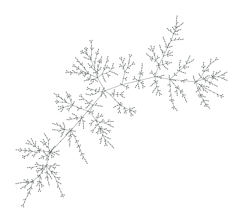
(a) $S$ is a path on $10$ nodes.

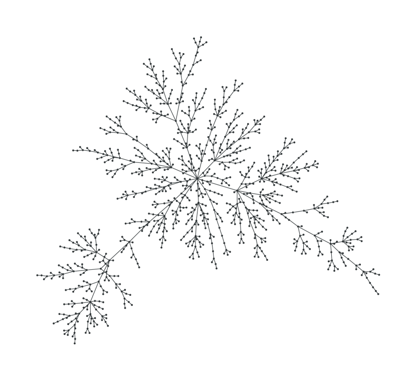
(b) $S$ is a star on $10$ nodes.

Figure 1. One sample from $\operatorname{UA}(1000,S)$ for two different seeds.

We inductively define a distribution on labelled trees: Let $\alpha\geq 0$, let $\operatorname{UA}_{\alpha}(k,S)=S$, and suppose that we are given $T_{n-1}\sim\operatorname{UA}_{\alpha}(n-1,S)$, where $V(T_{n-1})=\{u_{1},\dots,u_{n-1}\}$. Let $T_{n}\sim\operatorname{UA}_{\alpha}(n,S)$ be obtained from $T_{n-1}$ by adding a leaf labelled $u_{n}$ to $T_{n-1}$ and connecting it to a vertex $u\in\{u_{1},\dots,u_{n-1}\}$ with probability proportional to $\deg_{T_{n-1}}(u)^{\alpha}$. The distribution $\operatorname{UA}_{0}(n,P_{2})$, in which new leaves are attached to uniformly random vertices sequentially, is called the uniform attachment tree or random recursive tree, and is sometimes denoted by $\text{UA}(n)$ or $\text{URRT}(n)$ in the literature. The distribution $\operatorname{UA}_{1}(n,P_{2})$ is called the (linear) preferential attachment tree or Barabási-Albert model [2], sometimes denoted by $\text{PA}(n)$ in the literature. For $\alpha\in(0,1)$, $\operatorname{UA}_{\alpha}(n,P_{2})$ is called the sublinear preferential attachment tree, and when $\alpha>1$, it is called the superlinear preferential attachment tree. For general seeds $S$, the distributions above are said to be with seed $S$. In this paper, we are mostly concerned with $\operatorname{UA}_{0}(n,S)$, so we generally omit the subscript “0.” Moreover, if $T\sim\operatorname{UA}(n,S)$ and the distribution of $T$ is understood, we avoid repeating its distribution. See Figure 1 for a typical sample from $\operatorname{UA}(n,S)$ for different choices of $S$.

The vertices of the aforementioned trees are labelled; for a (rooted or unrooted) labelled tree $T$, let $T^{\circ}$ denote the isomorphism class of $T$, i.e., the operation $\circ$ “forgets” the labelling of $T$. With some abuse of notation, we refer to nodes of $T^{\circ}$ using their original labels in $T$. Of course, if $T\sim\operatorname{UA}(n,S)$ and nothing at all is assumed about $S$, it is always possible that $S=T$. Therefore, except if otherwise specified, we assume knowledge of the size of the seed in trying to locate it in $T^{\circ}$—our main goal is to detect $S$ in the unlabelled tree $\operatorname{UA}(n,S)^{\circ}$, given that $|S|=k$.

In general, sets of vertices which are made to include parts of the seed are referred to as (root-finding) vertex confidence sets. We reserve the letter $H$ for functions which map unlabelled trees to vertex confidence sets, and such functions are called root-finding algorithms. We also reserve the letter $K$ for the size of vertex confidence sets.

We assume that the reader is familiar with the basics of probability theory, including basic properties of standard random variables. We write $\operatorname{Beta}(\alpha,\beta)$ for a Beta distribution with parameters $\alpha,\beta$, i.e., the distribution supported on $[0,1]$ with density

$$f_{\alpha,\beta}(x)=\frac{1}{\mathrm{B}(\alpha,\beta)}x^{\alpha-1}(1-x)^{\beta-1},$$

where for $(\alpha_{1},\dots,\alpha_{k})\in\mathbb{R}^{k}_{+}$, we have $\mathrm{B}(\alpha_{1},\dots,\alpha_{k})=\frac{\prod_{i=1}^{k}\Gamma(\alpha_{i})}{\Gamma(\sum_{i=1}^{k}\alpha_{i})}$. We write $\operatorname{Dirichlet}(\alpha_{1},\dots,\alpha_{k})$ for the Dirichlet distribution, which is supported on the $k$-simplex

$$\mathopen{}\left\{(x_{1},\dots,x_{k})\colon\sum_{i=1}^{k}x_{i}=1\text{ and }x_{i}\in[0,1]\right\}\mathclose{}$$

and which has density

$$f_{\alpha_{1},\dots,\alpha_{k}}(x_{1},\dots,x_{k})=\frac{1}{\mathrm{B}(\alpha_{1},\dots,\alpha_{k})}\prod_{i=1}^{k}x_{i}^{\alpha_{i}-1}.$$

We often make use of the following fact about the distribution of sums of Dirichlet marginals: If $(X_{1},\dots,X_{k})\sim\operatorname{Dirichlet}(\alpha_{1},\dots,\alpha_{k})$, and $I\subseteq\{1,\dots,k\}$ is some index set, then

$$\sum_{i\in I}X_{i}\sim\operatorname{Beta}\mathopen{}\left(\sum_{i\in I}\alpha_{i},\sum_{i\in\{1,\dots,k\}\setminus I}\alpha_{i}\right)\mathclose{}.$$

1.4. Acknowledgements

The authors would like to thank the anonymous referees for their helpful comments and suggestions. Luc Devroye is supported by NSERC Grant A3456. Tommy Reddad is supported by an NSERC PGS D scholarship 396164433.

2. Finding a single vertex in the seed

2.1. An upper bound

For a tree $T$ and $u\in V(T)$, let

$$\psi_{T}(u)=\max_{v\in V(T)-u}|(T,u)_{v\downarrow}|,$$

so $\psi_{T}(u)$ is the size of the largest subtree of $T$ hanging off of the vertex $u$. We omit the subscript $T$ when the tree is understood.

Consider the strategy for picking central nodes from an unlabelled copy of $T\sim\operatorname{UA}(n,S)$ which works by simply picking the $K$ nodes minimizing the values of $\psi$. We will write $H^{*}_{\psi;K}(T^{\circ})$ for such a set of nodes. This strategy was first successfully introduced in [7], where $\psi$ is seen as a measure of node centrality, and in which it is shown that the root of $\operatorname{UA}(n)$ (which is the node labelled $u_{1}$) is likely to have low $\psi$ value. In fact, it is shown that this is also true for the root in preferential attachment trees. This centrality measure is further studied for root-finding in different settings [17, 18, 20].

Specifically, the result of [7, Theorem 3] has that for $K\geq(2.5/\varepsilon)\log(1/\varepsilon)$,

$$\operatorname{\mathbf{P}}_{T\sim\operatorname{UA}(n)}\Big{\{}u_{1}\in H^{*}_{\psi;K}(T^{\circ})\Big{\}}\geq 1-\frac{4\varepsilon}{1-\varepsilon},$$

and so, for $\varepsilon\leq 1/2$, $K(\varepsilon)\leq(80/\varepsilon)\log(1/\varepsilon)$. The following result indicates that $H^{*}_{\psi;K}$ also serves as a root-finding algorithm for seeded uniform attachment seeds, and offers an upper bound on the size of such vertex confidence sets.

Our proof relies on a few supporting lemmas and a classical result in the study of Pólya urns, whose proofs and statements are given in Appendix A.

Proposition 2.1.

There are universal constants $c,\varepsilon_{0}>0$ for which, if $\varepsilon\leq\varepsilon_{0}$ and

$$K\geq c(1/\varepsilon)^{2/k}\log(1/\varepsilon),$$

then

$$\operatorname{\mathbf{P}}\{|V(S)\cap H^{*}_{\psi;K}(T^{\circ})|\geq 1\}\geq 1-\varepsilon.$$

Theorem 1.1 follows immediately.

Proof of Proposition 2.1.

Figure 2. The seed $S$ has vertex set $\{u_{1},\dots,u_{5}\}$. The node $r=u_{3}$ is its unique centroid. The dashed edges form the set $\partial_{S}(r)$. The dotted lines outline the components of $S-\partial_{S}(r)$.

Let $\psi_{*}=\min\{\psi(u_{1}),\dots,\psi(u_{k})\}$. If for all $i>K$, $\psi(u_{i})>\psi_{*}$, then $V(S)$ intersects $H^{*}_{\psi;K}(T^{\circ})$, so

$$\operatorname{\mathbf{P}}\{V(S)\cap H^{*}_{\psi;K}(T^{\circ})=\emptyset\} \leq\operatorname{\mathbf{P}}\{\exists i>K\colon\psi(u_{i})\leq\psi_{*}\}$$

(4) $$\leq\operatorname{\mathbf{P}}\{\psi_{*}\geq nt\}+\operatorname{\mathbf{P}}\{\exists i>K\colon\psi(u_{i})\leq nt\},$$

where $t>0$ is to be specified later. It is a classical result that the seed $S$ has a centroid, i.e., a node $r$ whose removal splits the seed into components each of size at most $k/2$ [19]. Note that

$$\psi_{*}\leq\psi(r)\leq\max_{C\in\mathcal{C}(S-\partial_{S}(r))}\sum_{u\in C}|(T,S)_{u\downarrow}|,$$

where $\mathcal{C}(G)$ denotes the set of components of a graph $G$, and $\partial_{S}(r)$ denotes all of the edges of $S$ incident to $r$. Now, for any $C\in\mathcal{C}(S-\partial_{S}(r))$, we have by Lemma A.2 that

$$\frac{1}{n}\sum_{u\in C}|(T,S)_{u\downarrow}|\overset{d}{\to}\operatorname{Beta}(|C|,k-|C|),$$

as $n\to\infty$, so stochastically,

$$\frac{\psi_{*}}{n}\leq\max_{C\in\mathcal{C}(S-\partial_{S}(r))}\operatorname{Beta}(|C|,k-|C|)$$

and since $|C|\leq k/2$ uniformly because $r$ is a centroid, then each such beta random variable is stochastically smaller than a $\operatorname{Beta}(k/2,k/2)$ by Lemma A.3. See Figure 2. Let $f_{k/2,k/2}(x)$ be the density of a $\operatorname{Beta}(k/2,k/2)$ random variable. Using the bound

$$\sqrt{\frac{2\pi}{x}}\mathopen{}\left(\frac{x}{e}\right)\mathclose{}^{x}\leq\Gamma(x)\leq\sqrt{\frac{2\pi}{x}}\mathopen{}\left(\frac{x}{e}\right)\mathclose{}^{x}e^{\frac{1}{12x}},$$

which holds for all $x>0$ [13, Equation 5.6.1], we see that

$$\mathrm{B}(k/2,k/2)=\frac{\Gamma(k/2)^{2}}{\Gamma(k)}\geq 2^{-k}\cdot\frac{2}{e^{1/12}}\sqrt{\frac{2\pi}{k}}>3^{-k}$$

for all $k\geq 1$. Then,

$$\operatorname{\mathbf{P}}\{\psi_{*}\geq nt\} \leq k\operatorname{\mathbf{P}}\{\operatorname{Beta}(k/2,k/2)\geq t\}$$

$$=k\int_{t}^{1}f_{k/2,k/2}(x)\mathop{}\!\mathrm{d}x$$

$$\leq k3^{k}\int_{0}^{1-t}(x(1-x))^{k/2-1}\mathop{}\!\mathrm{d}x$$

$$\leq k3^{k}\int_{0}^{1-t}x^{k/2-1}\mathop{}\!\mathrm{d}x$$

$$=2(1-t)^{k/2}3^{k},$$

so we can pick $t=1-(1/9)(\varepsilon/4)^{2/k}$.

To summarize, we have shown that we can bound the first term in (4) by

$$\operatorname{\mathbf{P}}\{\psi_{*}/n\geq 1-(1/9)(\varepsilon/4)^{2/k}\}\leq\varepsilon/2.$$

For the second term, the argument is identical to that of [7, Theorem 3]. Indeed, if $T_{i}$ denotes the subgraph of $T$ containing the vertex $u_{i}$ after the removal of all edges between $\{u_{1},\dots,u_{K}\}$, then for any $i>K$,

$$\psi(u_{i})\geq\min_{1\leq j\leq K}\sum_{m=1,m\neq j}^{K}|T_{m}|,$$

and by Lemma A.2,

$$\frac{1}{n}\sum_{m=1,m\neq j}^{K}|T_{m}|\overset{d}{\to}\operatorname{Beta}(K-1,1)$$

as $n\to\infty$, so that

$$\operatorname{\mathbf{P}}\{\exists i>K\colon\psi(u_{i})\leq nt\} \leq K\operatorname{\mathbf{P}}\{\operatorname{Beta}(K-1,1)\leq t\}$$

$$=Kt^{K-1}$$

$$\leq Ke^{-(1/9)\varepsilon^{2/k}(K-1)},$$

and a little bit of arithmetic shows that we should pick

$$K\geq c(1/\varepsilon)^{2/k}\log(1/\varepsilon)$$

for universal constants $c,\varepsilon_{0}>0$, as long as $\varepsilon\leq\varepsilon_{0}$. ∎

Consequently, we see that

$$K^{*}(k,\ell,\varepsilon)\leq c(1/\varepsilon)^{2/k}\log(1/\varepsilon).$$

We note that $H^{*}_{\psi;K}(T^{\circ})$ can be computed in $O(n)$ time.

2.2. The maximum likelihood estimate

Given an unlabelled tree $T$, and a candidate seed $S$, define the likelihood function $\mathcal{L}_{T}(S)$ to be the probability of observing $T$ under $\operatorname{UA}(n,S)^{\circ}$, i.e.,

$$\mathcal{L}_{T}(S)=\operatorname{\mathbf{P}}_{T^{\prime}\sim\operatorname{UA}(n,S)}\{T^{\prime\circ}=T\},$$

and if $\mathcal{S}_{k,\ell}(T)$ denotes the set of all possible seeds in $T$ with $k$ vertices and $\ell$ leaves, the maximum likelihood estimate for $S$ is given by

$$S^{*}=\operatorname*{argmax}_{S\in\mathcal{S}_{k,\ell}(T)}\mathcal{L}_{T}(S).$$

Note that the subtrees $(T,S)_{u\downarrow}$ for $u\in V(S)$ are, conditionally on their sizes, independent random recursive trees:

Lemma 2.2.

Let $S$ be some seed, and $T\sim\operatorname{UA}(n,S)$, and $n_{u}\in\mathbb{N}$ for $u\in S$ be such that $\sum_{u\in S}n_{u}=n$. Then, conditionally on $|(T,S)_{u\downarrow}|=n_{u}$ for all $u\in S$, the trees $(T,S)_{u\downarrow}$ are independently distributed as $\operatorname{UA}(n_{u})$.

Proof sketch.

Any incoming node in the attachment process $\operatorname{UA}(n,S)$, conditionally upon connecting to $(T,S)_{u\downarrow}$ for some $u\in S$, will connect to a uniformly random node of $(T,S)_{u\downarrow}$. Conditioning on the event that $|(T,S)_{u\downarrow}|=n_{u}$, this precisely describes the uniform attachment tree $\operatorname{UA}(n_{u})$. ∎

As a consequence,

(5) $$\mathcal{L}_{T}(S)=\prod_{u\in V(S)}\mathcal{L}_{(T,S)_{u\downarrow}}(u),$$

where $\mathcal{L}_{(T,S)_{u\downarrow}}(u)$ is the likelihood of the tree $(T,S)_{u\downarrow}$ to be rooted at $u$, which is computed in [7, Section 3]. Specifically, as in [7], let $T$ be a rooted tree and $v$ a vertex of $T$, and $T_{1},\dots,T_{k}$ be the subtrees rooted at the children of $v$ listed in an arbitrary order, and $S_{1},\dots S_{L}$ be the isomorphism classes realized by these subtrees, define

$$\operatorname{Aut}(v,T)=\prod_{i=1}^{L}\bigl{|}\bigl{\{}j\in\{1,\dots,k\}\colon T_{j}^{\circ}=S_{i}\bigr{\}}\bigr{|}!.$$

Define also, for an unrooted unlabelled tree $T$,

$$\overline{\operatorname{Aut}}(u,T)=|\{v\in V(T)\colon(T,v)^{\circ}=(T,u)^{\circ}\}|,$$

i.e., $\overline{\operatorname{Aut}}(u,T)$ is the number of vertices $v\in V(T)$ such that the rooted trees $(T,v)$ and $(T,u)$ are isomorphic. Then,

$$\mathcal{L}_{T}(u)=\frac{|T|}{\overline{\operatorname{Aut}}(u,T)}\prod_{v\in V(T)}\frac{1}{|(T,u)_{v\downarrow}|\operatorname{Aut}(v,(T,u))},$$

so

(6) $$\mathcal{L}_{T}(S)=\prod_{u\in S}\frac{|(T,S)_{u\downarrow}|}{\overline{\operatorname{Aut}}(u,(T,S)_{u\downarrow})}\prod_{v\in(T,S)_{u\downarrow}}\frac{1}{|(T,S)_{v\downarrow}|\operatorname{Aut}(v,(T,S)_{u\downarrow})}.$$

In particular, this implies that the maximum likelihood estimate $S^{*}$ can be computed in polynomial time in $n$ for any fixed $k,\ell$, just as in the case when $k=1$ [7].

2.3. A vertex-confidence set with size subpolynomial in $(1/\varepsilon)$

For a tree $T$ and $u\in V(T)$, let

$$\varphi_{T}(u)=\prod_{v\in V(T)-\{u\}}|(T,u)_{v\downarrow}|,$$

omitting the $T$ subscript when $T$ is understood. We note, as noted by Bubeck, Devroye, and Lugosi in [7], that $1/\varphi$ resembles the expression of the likelihood in (6), so that nodes with small values of $\varphi$ should be likely candidates for the root. For $K\geq 1$, let $H^{*}_{\varphi;K}(T^{\circ})$ denote the set of $K$ vertices in $T^{\circ}$ minimizing their values of $\varphi$. In [7], it is shown that $H^{*}_{\varphi;K}$ serves as an effective root-finding algorithm for $T\sim\operatorname{UA}(n)$. We show that this is also the case when $T\sim\operatorname{UA}(n,S)$.

Proposition 2.3.

There are universal constants $c_{1},c_{2},c_{3},c_{4}>0$ such that if $k>c_{1}$, $\varepsilon\leq\exp\mathopen{}\left\{-c_{2}(\log k)^{11}\right\}\mathclose{}$, and

$$K\geq c_{3}\exp\mathopen{}\left\{c_{4}\frac{\log(1/\varepsilon)}{\log\log(1/\varepsilon)+\log\log k}\right\}\mathclose{},$$

then

$$\operatorname{\mathbf{P}}\{|V(S)\cap H^{*}_{\varphi;K}(T^{\circ})|\geq 1\}\geq 1-\varepsilon.$$

Proof.

Let $u$ be a vertex of $S$, and label each node $v\in(T,S)_{u\downarrow}$ using an extended version of the labelling scheme from [7], where every node of $T$ gets a label in

$$\mathbb{N}^{*}=\mathbb{N}\cup\mathbb{N}^{2}\cup\mathbb{N}^{3}\cup\dots,$$

such that if we write $v=(u,j_{1},\dots,j_{\ell})$, we mean that $v\in(T,S)_{u\downarrow}$, and that $v$ is the $j_{\ell}$-th child of $(u,j_{1},\dots,j_{\ell-1})$. Let also

$$s(v)=\sum_{i=1}^{\ell}(\ell-i+1)j_{i},$$

which we denote by $s$ when the node $v$ is understood. Let $u_{*}$ be the node of $S$ minimizing its value of $\varphi$ in $T$, so

$$\varphi(u_{*})=\min_{u\in S}\varphi(u).$$

Let $K$ and $K^{\prime}$ be related such that $K=|\{v\in(T,S)_{u_{*}\downarrow}\colon s(v)\leq 3K^{\prime}\}|$. Then,

$$\operatorname{\mathbf{P}}\{u_{*}\not\in H_{\varphi;K}(T^{\circ})\} \leq\operatorname{\mathbf{P}}\{\exists v\colon s(v)>3K^{\prime}\text{ and }\varphi(v)\leq\varphi(u_{*})\}$$

$$=\operatorname{\mathbf{P}}\{\exists u\in S,\,v\in(T,S)_{u\downarrow}\colon s(v)>3K^{\prime}\text{ and }\varphi(v)\leq\varphi(u_{*})\}$$

$$\leq\operatorname{\mathbf{P}}\{\exists u\in S,\,v\in(T,S)_{u\downarrow}\colon s(v)>3K^{\prime}\text{ and }\varphi(v)\leq\varphi(u)\}$$

(7) $$\leq\sum_{u\in V(S)}\operatorname{\mathbf{P}}\{\exists v\in(T,S)_{u\downarrow}\colon s(v)>3K^{\prime}\text{ and }\varphi(v)\leq\varphi(u)\},$$

By the arguments of [7, Page 9, Equation (9)], we have

$$\operatorname{\mathbf{P}}\{\exists v\in(T,S)_{u\downarrow}\colon s(v)>3K^{\prime}\text{ and }\varphi(v)\leq\varphi(u)\}$$

(8) $$\qquad\leq 2\sum_{v\in(T,S)_{u\downarrow}\colon s(v)\in(K^{\prime},3K^{\prime}]}\operatorname{\mathbf{P}}\{\varphi(v)\leq\varphi(u)\}.$$

Observe now that for $v=(u,j_{1},\dots,j_{\ell})$,

$$\varphi(v)\leq\varphi(u)\iff\prod_{i=1}^{\ell}|(T,S)_{(u,j_{1},\dots,j_{i})\downarrow}|\geq\prod_{i=1}^{\ell}(n-|(T,S)_{(u,j_{1},\dots,j_{i})\downarrow}|).$$

Observe that

(9) $$\frac{|(T,S)_{(u,j_{1},\dots,j_{i})\downarrow}|}{n}\overset{d}{\to}B\prod_{m=1}^{i}U_{j_{m},m},$$

as $n\to\infty$, where each $U_{j_{m},m}$ is an independent product of $j_{m}$ independent standard uniform random variables, and $B\sim\operatorname{Beta}(1,k-1)$. So, after dividing through by $n$,

(10) $$\operatorname{\mathbf{P}}\{\varphi(v)\leq\varphi(u)\}$$

$$\qquad\leq\operatorname{\mathbf{P}}\mathopen{}\left\{\prod_{i=1}^{\ell}B\prod_{m=1}^{i}U_{j_{m},m}\geq\prod_{i=1}^{\ell}\mathopen{}\left(1-B\prod_{m=1}^{i}U_{j_{m},m}\right)\mathclose{}\right\}\mathclose{}$$

$$\qquad=\operatorname{\mathbf{P}}\mathopen{}\left\{\prod_{i=1}^{\ell}\prod_{m=1}^{i}U_{j_{m},m}\geq\prod_{i=1}^{\ell}\mathopen{}\left(\frac{1}{B}-\prod_{i=1}^{i}U_{j_{m},m}\right)\mathclose{}\right\}\mathclose{}$$

(11) $$\qquad\leq\operatorname{\mathbf{P}}\mathopen{}\left\{\prod_{i=1}^{\ell}\prod_{m=1}^{i}U_{j_{m},m}\geq t\right\}\mathclose{}+\operatorname{\mathbf{P}}\mathopen{}\left\{\prod_{i=1}^{\ell}\mathopen{}\left(\frac{1}{B}-\prod_{m=1}^{i}U_{j_{m},m}\right)\mathclose{}\leq t\right\}\mathclose{},$$

where $t>0$ is to be specified later. The first inequality above follows by the portmanteau lemma and the convergence in distribution noted in (9).

In [7, Lemma 1], it is shown that

$$\operatorname{\mathbf{P}}\mathopen{}\left\{\prod_{i=1}^{\ell}\prod_{m=1}^{i}U_{j_{m},m}\geq t\right\}\mathclose{}\leq\exp\mathopen{}\left\{-\sqrt{s/2}\log\mathopen{}\left(\frac{s}{e\log(1/t)}\right)\mathclose{}\right\}\mathclose{}.$$

On the other hand, observing that $1-e^{-x}\geq(1/2)\min\{x,1\}$ for all $x\geq 0$, we have

$$\operatorname{\mathbf{P}}\mathopen{}\left\{\prod_{i=1}^{\ell}\mathopen{}\left(\frac{1}{B}-\prod_{m=1}^{i}U_{j_{m},m}\right)\mathclose{}\leq t\right\}\mathclose{}$$

$$\qquad\leq\operatorname{\mathbf{P}}\mathopen{}\left\{\prod_{i=1}^{\ell}\mathopen{}\left(\frac{1}{B}-1+\frac{1}{2}\min\mathopen{}\left\{\sum_{m=1}^{i}\log(1/U_{j_{m},m}),1\right\}\mathclose{}\right)\mathclose{}\leq t\right\}\mathclose{}$$

(12) $$\qquad\leq\operatorname{\mathbf{P}}\mathopen{}\left\{\prod_{i=1}^{\ell}\mathopen{}\left(\frac{1}{B}-1+\frac{1}{2}\min\mathopen{}\left\{\sum_{m=1}^{i}E_{m},1\right\}\mathclose{}\right)\mathclose{}\leq t\right\}\mathclose{},$$

where $E_{1},E_{2},\dots$ are independent standard exponential random variables. By the inequality of arithmetic and geometric means,

$$(\ref{eq:rhs-2}) \leq\operatorname{\mathbf{P}}\mathopen{}\left\{2^{\ell/2}\mathopen{}\left(\frac{1}{B}-1\right)\mathclose{}^{\ell/2}\mathopen{}\left(\prod_{i=1}^{\ell}\min\mathopen{}\left\{\sum_{m=1}^{i}E_{m},1\right\}\mathclose{}\right)\mathclose{}^{1/2}\leq t\right\}\mathclose{}$$

(13) $$\leq\operatorname{\mathbf{P}}\mathopen{}\left\{2^{\ell}\mathopen{}\left(\frac{1}{B}-1\right)\mathclose{}^{\ell}X\leq t^{2}\right\}\mathclose{},$$

where $X$ is defined by

$$X=\prod_{i=1}^{\infty}\min\mathopen{}\left\{\sum_{m=1}^{i}E_{m},1\right\}\mathclose{}.$$

Then, for $q>1$ to be specified,

$$(\ref{eq:rhs-3})\leq\operatorname{\mathbf{P}}\mathopen{}\left\{\frac{B}{1-B}\geq\frac{2}{q^{1/\ell}}\right\}\mathclose{}+\operatorname{\mathbf{P}}\mathopen{}\left\{X\leq\frac{t^{2}}{q}\right\}\mathclose{}.$$

By [7, Lemma 2], we know that

(14) $$\operatorname{\mathbf{P}}\mathopen{}\left\{X\leq\frac{t^{2}}{q}\right\}\mathclose{}\leq\frac{6t^{1/2}}{q^{1/4}},$$

and it is also known that

(15) $$\operatorname{\mathbf{P}}\mathopen{}\left\{\frac{B}{1-B}\geq\frac{2}{q^{1/\ell}}\right\}\mathclose{}=\frac{1}{(1+2/q^{1/\ell})^{k-1}}\leq\exp\mathopen{}\left\{-\frac{k-1}{q^{1/\ell}}\right\}\mathclose{},$$

where the inequality follows since $q>1$, where here we have used that $\frac{1}{1+x}\leq e^{-x/2}$ for $0\leq x\leq 2$. Optimizing a choice of $q$ in (14) against (15), one can see that when $t>(1/36)e^{-2(k-1)}$,

$$(\ref{eq:rhs-3}) \leq 12t^{1/2}\mathopen{}\left(\frac{\log(1/6t^{1/2})+(\ell/4)\log\mathopen{}\left(\frac{k-1}{\log(1/6t^{1/2})}\right)\mathclose{}}{k-1}\right)\mathclose{}^{\ell/4}$$

$$\leq 12t^{1/2}\mathopen{}\left(\frac{\log(1/6t^{1/2})+(\sqrt{2s}/4)\log\mathopen{}\left(\frac{k-1}{\log(1/6t^{1/2})}\right)\mathclose{}}{k-1}\right)\mathclose{}^{\sqrt{2s}/4},$$

where we used the fact that

$$s=\sum_{i=1}^{\ell}(\ell-i+1)j_{i}\geq\ell^{2}/2.$$

It remains to make an optimal of choice of $t$. If we pick $t$ such that

$$\log(1/6t^{1/2})=s^{0.6}-(\sqrt{2s}/4)\log(k-1),$$

it can be shown that if $s>10^{12}$, $t<1/6^{6}$, and $\log(1/6t^{1/2})>s^{0.6}/2$, then

$$(\ref{eq:failure-prob-v-r})\leq 2\exp\mathopen{}\left\{-\sqrt{s/2}\log\mathopen{}\left((1/25)s^{0.3}\log(k-1)\right)\mathclose{}\right\}\mathclose{}.$$

Recall the union bound (8),

$$\operatorname{\mathbf{P}}\{u_{*}\not\in H_{\varphi;K}(T^{\circ})\}\leq 2\sum_{u\in V(S)}\mathopen{}\left(\sum_{v\in(T,S)_{u\downarrow}\colon s(v)\in(K^{\prime},3K^{\prime}]}\operatorname{\mathbf{P}}\{\varphi(v)\leq\varphi(u)\}\right)\mathclose{}.$$

We know that for any $u\in V(S)$,

$$|\{v\in(T,S)_{u\downarrow}\colon s(v)\in(K^{\prime},3K^{\prime}]\}|\leq 3K^{\prime}\exp\{\pi\sqrt{2K^{\prime}}\},$$

(see [7, Page 8, Equation (6)]) and by the conditions imposed on $s$ and $k$,

$$6kK^{\prime}\exp\{\pi\sqrt{2K^{\prime}}\}\leq 6\exp\{11\sqrt{K^{\prime}}\},$$

and therefore,

$$\operatorname{\mathbf{P}}\{u_{*}\not\in H_{\varphi;K}(T^{\circ})\} \leq 6\exp\mathopen{}\left\{11\sqrt{K^{\prime}}-\sqrt{K^{\prime}/2}\log\mathopen{}\left((1/25)K^{\prime 0.3}\log(k-1)\right)\mathclose{}\right\}\mathclose{}$$

$$\leq 6\exp\mathopen{}\left\{-(1/2)\sqrt{K^{\prime}}\log\mathopen{}\left((1/25)K^{\prime 0.3}\log(k-1)\right)\mathclose{}\right\}\mathclose{}$$

for $K^{\prime}>10^{77}$, which holds for $k>10^{10^{8}}$. In order to make this probability at most $\varepsilon$, we can pick for some universal constant $c_{1}>0$,

$$\sqrt{K^{\prime}}=c_{1}\frac{\log(1/\varepsilon)}{\log\log(1/\varepsilon)+\log\log k}.$$

In order to satisfy the condition that $\log(1/6t^{1/2})>s^{0.6}/2$, this requires that for some constant $c_{2}>0$,

$$\varepsilon<\exp\mathopen{}\left\{-c_{2}(\log k)^{11}\right\}\mathclose{}.$$

In this case, there are universal constants $c_{3},c_{4}>0$ such that

$$K =|\{v\in(T,S)_{u_{*}\downarrow}\colon s(v)\leq 3K^{\prime}\}$$

$$\leq c_{3}\exp\mathopen{}\left\{c_{4}\frac{\log(1/\varepsilon)}{\log\log(1/\varepsilon)+\log\log k}\right\}\mathclose{}.\qed$$

2.4. A lower bound

To obtain a lower bound on $K^{*}(k,\ell,\varepsilon)$, one can use the likelihood of an observation under $\operatorname{UA}(n,S)$, computed in Section 2.2, and as in [7, Theorem 4], one can then construct a family of probable trees whose maximum likelihood estimate for $K$-sized sets to intersect the seed will avoid every node of the seed—the right choice for $K$ so that such a tree appears with probability at least $\varepsilon$ would then give a lower bound on $K^{*}(k,\ell,\varepsilon)$. Instead of this lengthy retelling, we use Lemma 2.2 to show how any lower bound on $K(\varepsilon)$ also offers a lower bound on $K^{*}(k,\ell,\varepsilon)$.

Define $H^{*}_{K,k}(T^{\circ})$ to be the maximum likelihood estimate for the set of size $K$ most likely to contain at least one node of the true seed of $T\sim\operatorname{UA}(n,S)$, given $|S|=k$ and $|L(S)|=\ell$:

$$H^{*}_{K,k,\ell}(T^{\circ})=\operatorname*{argmax}_{H^{*}\in V(T)^{(K)}}\sum_{S^{\prime}\in\mathcal{S}_{k,\ell}(T)\colon|V(S^{\prime})\cap H^{*}|\geq 1}\mathcal{L}_{T^{\circ}}(S^{\prime}).$$

In order to prove that $K^{*}(k,\ell,\varepsilon)\geq K$ for some particular $K$, it suffices to show that for some specific $n$, and for all $S$ with $|S|=k$ and $|L(S)|=\ell$,

$$\operatorname{\mathbf{P}}_{T\sim\operatorname{UA}(n,S)}\{V(S)\cap H_{K,k,\ell}^{*}(T^{\circ})=\emptyset\}\geq\varepsilon.$$

Proof of Theorem 1.3.

Let $m=k^{2}K$. For brevity, let $M_{u}=|(T,S)_{u\downarrow}|$, and let $M_{*}=\min_{u\in S}M_{u}$. By Lemma A.1,

$$\frac{M_{*}}{n}\overset{d}{\to}\frac{\operatorname{Beta}(1,k-1)}{k}$$

as $n\to\infty$. Then,

$$\operatorname{\mathbf{P}}_{T\sim\operatorname{UA}(m,S)}\{M_{*}/m>1/k^{2}\} \geq\liminf_{n\to\infty}\operatorname{\mathbf{P}}_{T\sim\operatorname{UA}(n,S)}\{M_{*}/n>1/k^{2}\}$$

$$\geq\operatorname{\mathbf{P}}\{\operatorname{Beta}(1,k-1)>1/k\}$$

$$=(1-1/k)^{k-1}$$

$$\geq e^{-1}.$$

Let

$$\mathcal{M}=\mathopen{}\left\{(m_{u}\colon u\in S)\colon m_{u}\in\mathbb{N},\,\sum_{u\in S}m_{u}=m,\,\min_{u\in S}m_{u}>\frac{m}{k^{2}}\right\}\mathclose{}.$$

Upon conditioning,

$$\operatorname{\mathbf{P}}_{T\sim\operatorname{UA}(m,S)}\{V(S)\cap H_{K,k,\ell}^{*}(T^{\circ})=\emptyset\}$$

$$\qquad\geq\operatorname{\mathbf{P}}\{M_{*}/m>1/k^{2}\}$$

$$\qquad\hphantom{\geq}\sum_{(m_{u}\colon u\in S)\in\mathcal{M}}\operatorname{\mathbf{P}}\mathopen{}\left\{\bigcap_{u\in S}[u\not\in H_{K,k,\ell}^{*}(T^{\circ})\cap(T,S)_{u\downarrow}]\;\middle|\;\bigcap_{u\in S}[M_{u}=m_{u}]\right\}\mathclose{}$$

$$\qquad\geq e^{-1}\sum_{(m_{u}\colon u\in S)\in\mathcal{M}}\mathopen{}\left(\prod_{u\in S}\operatorname{\mathbf{P}}\Bigl{\{}u\not\in H_{K,k,\ell}^{*}((T,S)_{u\downarrow}^{\circ})\mathrel{\Big{|}}M_{u}=m_{u}\Bigr{\}}\right)\mathclose{}$$

$$\qquad\geq e^{-1}\Bigl{(}\operatorname{\mathbf{P}}_{T\sim\operatorname{UA}(K+1)}\{u_{1}\not\in H_{K,1}^{*}(T^{\circ})\}\Bigr{)}^{k},$$

where this last line follows from the optimality of $H^{*}_{K,1}((T,S)_{u\downarrow}^{\circ})$ as a root estimator in $(T,S)_{u\downarrow}^{\circ}$, and since conditionally upon $M_{u}=m_{u}$, $(T,S)_{u\downarrow}$ is distributed as $\operatorname{UA}(m_{u})$ by Lemma 2.2. By definition, if $K<K((e\varepsilon)^{1/k})$, then the probability that $H^{*}_{K,k,\ell}(T^{\circ})$ avoids $V(S)$ exceeds $\varepsilon$. ∎

Corollary 1.4 follows immediately.

3. Finding all seed vertices

3.1. Upper bounds

3.1.1. A familiar strategy

We can also use the strategy $H^{*}_{\psi;K}$ of [7] and Section 2.1 to get all the nodes of $S$; in this section, when the procedure is used to find all nodes of the seed, we omit the asterisk for notational consistency. More specifically, we study the smallest choice of $K$ for which $H_{\psi;K}$ contains all nodes of $S$ with probability at least $1-\varepsilon$, and such a choice will give an upper bound on $K(k,\ell,\varepsilon)$.

If $\psi(u)=|(T,u)_{v\downarrow}|$ for $v$ adjacent to $u$, we will say that $\psi(u)$ is witnessed at $v$.

Proposition 3.1.

There are universal constants $c,\varepsilon_{0}>0$ such that, if $\varepsilon\leq\varepsilon_{0}$ and

$$K\geq(ck\ell/\varepsilon)\log(k\ell/\varepsilon),$$

then

$$\operatorname{\mathbf{P}}\{V(S)\subseteq H_{\psi;K}(T^{\circ})\}\geq 1-\varepsilon.$$

Proof.

Figure 3. The seed $S$ has vertex set $\{u_{1},\dots,u_{5}\}$. Suppose that $\psi^{*}=\psi(u_{1})$. Then, $\psi^{*}$ is witnessed at $u_{2}$, and $\psi^{*}$ correponds to the size of the outlined subgraph.

The proof is similar to that of Proposition 2.1. Write

$$\psi^{*}=\max\{\psi(u_{1}),\dots,\psi(u_{k})\}.$$

Observe that if for all $i>K$, $\psi(u_{i})>\psi^{*}$, then $V(S)\subseteq H_{\psi;K}(T^{\circ})$. So,

(16) $$\operatorname{\mathbf{P}}\{V(S)\not\subseteq H_{\psi;K}(T^{\circ})\}\leq\operatorname{\mathbf{P}}\{\psi^{*}\geq nt\}+\operatorname{\mathbf{P}}\{\exists i>K\colon\psi(u_{i})\leq nt\}$$

for $t>0$ to be specified. We handle the first term in (16): Suppose that $\psi^{*}$ is attained by $u\in V(S)$ and witnessed by its child $v\not\in V(S)$, i.e.,

$$\psi^{*}=\psi(u)=|(T,u)_{v\downarrow}|,$$

Then, $u$ has a neighbour $w\in V(S)$, and

$$\psi(w)\geq|(T,w)_{u\downarrow}|>|(T,u)_{v\downarrow}|=\psi(u),$$

so $\psi(u)$ cannot be maximum. Thus, $\psi^{*}$ must be witnessed by a node of $V(S)$, and in particular, one can iterate the above motion to see that $\psi^{*}$ must be attained by a leaf of $S$ and witnessed by its unique neighbour in $S$, so

$$\psi^{*}=\max_{u\in L(S)}\sum_{v\in V(S)-u}|(T,S)_{v\downarrow}|.$$

See Figure 3 for an illustration. By Lemma A.2, for any $u\in L(S)$,

$$\frac{1}{n}\sum_{v\in V(S)-u}|(T,S)_{v\downarrow}|\overset{d}{\to}\operatorname{Beta}(k-1,1),$$

as $n\to\infty$, so

$$\operatorname{\mathbf{P}}\{\psi^{*}\geq nt\} \leq\operatorname{\mathbf{P}}\mathopen{}\left\{\exists u\in L(S)\colon\sum_{v\in V(S)-u}|(T,S)_{v\downarrow}|\geq nt\right\}\mathclose{}$$

$$\leq\ell\operatorname{\mathbf{P}}\{\operatorname{Beta}(k-1,1)\geq t\}$$

$$=\ell(1-t^{k-1}).$$

We can make this at most $\varepsilon/2$ by choosing $t=(1-\varepsilon/(2\ell))^{1/(k-1)}$.

For the second term in (16), the argument is again identical to that of [7, Theorem 3], and we can say that

$$\operatorname{\mathbf{P}}\{\exists i>K\colon\psi(u_{i})\leq nt\}\leq Kt^{K-1}\leq Ke^{-\frac{\varepsilon(K-1)}{2(k-1)\ell}}.$$

Picking $K\geq(ck\ell/\varepsilon)\log(k\ell/\varepsilon)$ for some constant $c>0$ gives the desired result, as long as $\varepsilon\leq\varepsilon_{0}$ for some constant $\varepsilon_{0}>0$. ∎

Again, the set $H_{\psi;K}(T^{\circ})$ can be computed in $O(n)$ time. We show in Lemma 4.2 that the result of Theorem 1.5 involves the right order for $K$ for the strategy given by $H_{\psi;K}$, up to logarithmic factors: When $K\leq k\ell/(4\varepsilon)$, then with probability at least $\varepsilon$, at least one leaf of $S$ is also a leaf of $T\sim\operatorname{UA}(K,S)$, and any leaf of $T$ maximizes the value of $\psi$.

3.1.2. A reduction to intersection testing

We now consider an alternative procedure for locating all nodes of the seed, which sometimes requires fewer nodes than $H_{\psi;K}$ to succeed with probability $1-\varepsilon$. We define the set $H_{\phi;K,k,\ell,\varepsilon}(T^{\circ})$ as follows:

1. Let $H^{*}$ be a set of size $K^{*}(k,\ell,\varepsilon/2)$ which intersects the seed with probability at least $1-\varepsilon/2$;

2. For each $u\in H^{*}$, traverse the tree $T$ in a depth-first manner around $u$;

3. When exploring $v\in T$, add $v$ to $H_{\phi;K,k,\ell,\varepsilon}(T^{\circ})$ if $|(T,u)_{v\downarrow}|\geq n\varepsilon/(2k\ell)$, and stop exploring this path otherwise. Stop at any point if the size of the set exceeds $K$.

If we can prove that $H_{\phi;K,k,\ell,\varepsilon}(T^{\circ})$ includes the whole seed with probability at least $1-\varepsilon$, and that $K$ is sufficiently large, we obtain an upper bound on $K(k,\ell,\varepsilon)$.

Proposition 3.2.

If $K\geq(2k\ell/\varepsilon)K^{*}(k,\ell,\varepsilon/2)$, then

$$\operatorname{\mathbf{P}}\{V(S)\subseteq H_{\phi;K,k,\ell,\varepsilon}(T^{\circ})\}\geq 1-\varepsilon.$$

Proof.

We show the failure probability is small enough:

$$\operatorname{\mathbf{P}}\{V(S)\not\subseteq H_{\phi;K,k,\ell,\varepsilon}(T^{\circ})\}\leq\operatorname{\mathbf{P}}\biggl{\{}V(S)\cap H^{*}=\emptyset\biggr{\}}+\operatorname{\mathbf{P}}\biggl{\{}\min_{u\in L(S)}|(T,S)_{u\downarrow}|<\frac{n\varepsilon}{2k\ell}\biggr{\}}.$$

The first term is at most $\varepsilon/2$ by definition. For the second term, note that

$$\frac{\min_{u\in L(S)}|(T,S)_{u\downarrow}|}{n}\overset{d}{\to}\frac{\operatorname{Beta}(1,k-1)}{\ell},$$

as $n\to\infty$ by Lemma A.1, so

$$\operatorname{\mathbf{P}}\biggl{\{}\min_{u\in L(S)}|(T,S)_{u\downarrow}|<\frac{n\varepsilon}{2k\ell}\biggr{\}} \leq\operatorname{\mathbf{P}}\biggl{\{}\operatorname{Beta}(1,k-1)\leq\frac{\varepsilon}{2k}\biggr{\}}$$

$$=1-\mathopen{}\left(1-\frac{\varepsilon/2}{k}\right)\mathclose{}^{k-1}$$

$$\leq 1-e^{-\varepsilon/2}$$

$$\leq\varepsilon/2,$$

as desired. Finally, for $u$ fixed, there are at most $2k\ell/\varepsilon$ nodes $v$ such that $|(T,u)_{v\downarrow}|\geq n\varepsilon/(2k\ell)$, so $K$ is indeed large enough to include all desired nodes. ∎

By a remark in Section 2.2, the set $H^{*}$ in the above construction can be computed in polynomial time, so $H_{\phi;K,k,\ell,\varepsilon}(T^{\circ})$ can be computed in polynomial time. Theorem 1.5 follows immediately from Proposition 3.1 and Proposition 3.2.

3.2. Lower bounds

By (1), we have the same lower bound on $K(k,\ell,\varepsilon)$ as in Theorem 1.3, i.e.,

Corollary 3.3.

There are universal constants $c_{1},c_{2},c_{3}>0$, and such that if $\varepsilon\leq e^{-c_{1}k}$, then

$$K(k,\ell,\varepsilon)\geq c_{2}\exp\mathopen{}\left\{c_{3}\sqrt{\frac{\log(1/\varepsilon)}{k}}\right\}\mathclose{}.$$

Unlike the case for $K^{*}(k,\ell,\varepsilon)$, we do not know that $K(k,\ell,\varepsilon)$ is at most linear in $k$ when $\varepsilon>e^{-ck}$; our best upper bound from Theorem 1.5 says that $K(k,\ell,\varepsilon)$ is at most exponential in $k$, while the lower bound from Corollary 3.3 does not apply. We thus search for a lower bound on $K(k,\ell,\varepsilon)$ which applies in the regime when $\varepsilon$ is large.

As in Section 2.4, define $H_{K,k,\ell}(T^{\circ})$ to be the set of size $K$ most likely to contain all the nodes of the true seed of $T\sim\operatorname{UA}(n,S)$, given $|S|=k$ and $|L(S)|=\ell$:

$$H_{K,k,\ell}(T^{\circ})=\operatorname*{argmax}_{H\in V(T)^{(K)}}\sum_{S^{\prime}\in\mathcal{S}_{k,\ell}(T)\colon V(S^{\prime})\subseteq H}\mathcal{L}_{T^{\circ}}(S^{\prime}).$$

If $\varepsilon$ is at least some positive constant, then $K(k,\ell,\varepsilon)\leq ck\ell$ for some constant $c>0$ by Theorem 1.5. We noted in Section 3.1.1, as a result of Lemma 4.2, that if $H_{\psi;K}$ were the optimal strategy for picking $K$ nodes to include the whole seed with probability at least $1-\varepsilon$, then $k\ell/(4\varepsilon)$ is roughly a lower bound on the size of such a vertex confidence set. We know that $H_{\psi;K}$ is not in fact the optimal strategy, but one can understand it to be a relaxation of the optimal strategy $H_{K,k,\ell}$. We thus make the following conjecture, which expresses our belief that $H_{\psi;K}$ is “close enough” to $H_{K,k,\ell}$ when $\varepsilon$ is large.

Conjecture 3.4.

There are universal constants $c_{1},c_{2},\varepsilon_{0}>0$ such that if $k,\ell>c_{1}$, then,

$$K(k,\ell,\varepsilon_{0})\geq c_{2}k\ell.$$

4. Finding all leaves given the skeleton

For a seed $S$, write $R(S)=S-L(S)$ for the skeleton of $S$, or simply $R$ when $S$ is understood. For an integer $i\geq 1$, let $\mathcal{T}_{i}$ denote the set of trees in which a set of $i$ labelled vertices form a connected subgraph, and in which all other vertices are unlabelled. For a given labelled tree $T$ and a set $A\in V(T)^{(i)}$, let $T^{(A)}\in\mathcal{T}_{i}$ be the tree in which all labels are forgotten except for those of $A$. Consider now the optimal size

$$K^{\prime}(k,\ell,\varepsilon)=\min\mathopen{}\left\{m\colon\begin{array}[]{l}\displaystyle\exists H^{\prime}_{m,k,\ell,\varepsilon}\colon\mathcal{T}_{k-\ell}\to V(\mathcal{T}_{k-\ell})^{(m)},\text{ such that}\\ \displaystyle\min\limits_{\begin{subarray}{c}S\colon|S|=k\\ |L(S)|=\ell\end{subarray}}\operatorname{\mathbf{P}}_{T\sim\operatorname{UA}(n,S)}\{L(S)\subseteq H^{\prime}_{m,k,\ell,\varepsilon}(T^{(R)})\}\geq 1-\varepsilon\end{array}\right\}\mathclose{}.$$

be the optimal size of a set which, given the position of the skeleton of the seed, the size of the seed, and its number of leaves, will locate all of its true leaves with probability at least $1-\varepsilon$.

As in Section 2 and Section 3, we find an upper bound on $K^{\prime}(k,\ell,\varepsilon)$ by exhibiting an algorithm which, given $k,\varepsilon$ and $R$, returns a set of vertices which contains all of $L(S)$ with probability at least $1-\varepsilon$.

Let $\psi(u)=|(T,R)_{u\downarrow}|$, and let $H^{\prime}_{\psi;K}(T^{(R)})$ be the set of $K$ vertices $u\in N(R)$ maximizing their value of $\psi$. This estimator for $L(S)$ is slightly different than those for $V(S)$ seen in Section 2 and Section 3. Indeed, allowing ourselves to assume $R$ significantly improves our chances at correctly guessing the rest of $S$. Specifically, if $k$ is constant, the dependence of $K^{\prime}(k,\ell,\varepsilon)$ upon $1/\varepsilon$ is shown to be logarithmic, while the result of Theorem 1.3 has that, for sufficiently small $\varepsilon$, $K^{*}(k,\ell,\varepsilon)$ is superpolylogarithmic in $1/\varepsilon$.

Proposition 4.1.

If

$$K\geq\ell+2(k-\ell)\log\mathopen{}\left((3\ell/\varepsilon)\log\mathopen{}\left(\frac{3(k-\ell)}{\varepsilon}\right)\mathclose{}\right)\mathclose{}+(7/6)\log\mathopen{}\left(\frac{3(k-\ell)}{\varepsilon}\right)\mathclose{}$$

then $\operatorname{\mathbf{P}}\{L(S)\subseteq H^{\prime}_{\psi;K}(T^{(R)})\}\geq 1-\varepsilon$.

Proof.

Let $v_{1},v_{2},\dots$ be the chronological sequence of nodes attaching to $R$, where $\{v_{1},v_{2},\dots,v_{\ell}\}=L(S)$ ordered arbitrarily. Write $\psi_{*}=\min_{u\in L(S)}\psi(u)$. If for all $i>K$, $\psi(v_{i})<\psi_{*}$, then $L(S)\subseteq H^{\prime}_{\psi;K}(T^{(R)})$. So

(17) $$\operatorname{\mathbf{P}}\{L(S)\not\subseteq H^{\prime}_{\psi;K}(T^{(R)})\}\leq\operatorname{\mathbf{P}}\{\psi_{*}\leq tn\}+\operatorname{\mathbf{P}}\{\exists i>K\colon\psi(v_{i})\geq tn\}$$

for $t>0$ to be specified. Observe that $\psi_{*}/n$ converges in distribution to $\operatorname{Beta}(1,k-1)/\ell$ as $n\to\infty$, so

$$\operatorname{\mathbf{P}}\{\psi_{*}\leq tn\} \leq\operatorname{\mathbf{P}}\{\operatorname{Beta}(1,k-1)\leq t\ell\}$$

$$\leq t\ell(k-1)$$

$$\leq\varepsilon/3$$

if we choose $t=\varepsilon/(3\ell(k-1))$ .

It remains to handle the second term in (17). Let $N$ be the (random) time at which $v_{K}$ is inserted, i.e., $v_{K}=u_{N}$. Let $T_{u}$ be the component of $T$ containing $u$ after the removal of all edges between $\{u_{1},\dots,u_{N}\}$. Any node $v_{i}$ with $i>K$ is part of $T_{u}$ for some $u\in R$. Since for any $u\in R$, $|T_{u}|/n$ converges in distribution to $\operatorname{Beta}(1,N-1)$ as $n\to\infty$,

$$\operatorname{\mathbf{P}}\{\exists i>K\colon\psi(v_{i})\geq tn\}$$

$$\qquad\leq\operatorname{\mathbf{P}}\{\exists u\in R\colon|T_{u}|\geq nt\}$$

$$\qquad\leq(k-\ell)\operatorname{\mathbf{P}}\{\operatorname{Beta}(1,N-1)\geq t\}$$

(18) $$\qquad\leq(k-\ell)\operatorname{\mathbf{P}}\{\operatorname{Beta}(1,N-1)\geq t\mid N\geq s\}+(k-\ell)\operatorname{\mathbf{P}}\{N\leq s\},$$

where $s>0$ is to be specified. Conditionally upon $N\geq s$, $\operatorname{Beta}(1,s-1)$ stochastically dominates $\operatorname{Beta}(1,N-1)$ by Lemma A.4, so

$$(k-\ell)\operatorname{\mathbf{P}}\{\operatorname{Beta}(1,N-1)\geq t\mid N\geq s\} \leq(k-\ell)\operatorname{\mathbf{P}}\{\operatorname{Beta}(1,s-1)\geq t\}$$

$$=(k-\ell)(1-t)^{s-1}$$

$$\leq(k-\ell)e^{-t(s-1)},$$

which is less than $\varepsilon/3$ if we choose

$$s=1+(1/t)\log\mathopen{}\left(\frac{3(k-\ell)}{\varepsilon}\right)\mathclose{}=1+\frac{3\ell(k-1)}{\varepsilon}\log\mathopen{}\left(\frac{3(k-\ell)}{\varepsilon}\right)\mathclose{}.$$

For the second term in (18), observe that

$$\operatorname{\mathbf{P}}_{T\sim\operatorname{UA}(n,S)}\{N\leq s\}\leq\operatorname{\mathbf{P}}_{T\sim\operatorname{UA}(s,S)}\{\deg(R)\geq K\},$$

where

$$\deg(R)=\ell+\sum_{i=k+1}^{s}\mathbf{1}\{u_{i}\text{ connects to $R$}\}$$

and each such indicator is independent. Clearly, for any $i\geq k+1$,

$$\mathbf{1}\{u_{i}\text{ connects to $R$}\}\sim\operatorname{Bernoulli}\mathopen{}\left(\frac{k-\ell}{i-1}\right)\mathclose{},$$

so writing $H_{m}=\sum_{i=1}^{m}1/i$ for the $m$-th Harmonic number,

$$\operatorname{\mathbf{E}}\{\deg(R)\}=\ell+(k-\ell)(H_{s-1}-H_{k-1}).$$

Picking

$$K\geq\ell+(k-\ell)(H_{s-1}-H_{k-1})+\delta$$

for $\delta>0$ to be specified, we have by Bernstein’s inequality [3, 6],

$$\operatorname{\mathbf{P}}\{\deg(R)\geq K\}$$

$$\qquad\leq\operatorname{\mathbf{P}}\mathopen{}\left\{\mathopen{}\left[\sum_{i=k+1}^{s}\operatorname{Bernoulli}\mathopen{}\left(\frac{k-\ell}{i-1}\right)\mathclose{}\right]\mathclose{}-(k-\ell)(H_{s-1}-H_{k-1})\geq\delta\right\}\mathclose{}$$

$$\qquad\leq\exp\mathopen{}\left\{-\frac{\delta^{2}}{2(k-\ell)(H_{s-1}-H_{k-1})+2\delta/3}\right\}\mathclose{}$$

$$\qquad\leq\exp\mathopen{}\left\{-\frac{\delta^{2}}{2(k-\ell)\log\mathopen{}\left(\frac{s-1}{k}\right)\mathclose{}+2\delta/3}\right\}\mathclose{}.$$

Some arithmetic shows that picking

$$\delta=(2/3)\log\mathopen{}\left(\frac{3(k-\ell)}{\varepsilon}\right)\mathclose{}+\sqrt{2(k-\ell)\log\mathopen{}\left(\frac{s-1}{k}\right)\mathclose{}\log\mathopen{}\left(\frac{3(k-\ell)}{\varepsilon}\right)\mathclose{}}$$

suffices to have

$$\operatorname{\mathbf{P}}\{\deg(R)\geq K\}\leq\frac{\varepsilon}{3(k-\ell)},$$

and therefore, in (18),

$$(k-\ell)\operatorname{\mathbf{P}}\{N\leq s\}\leq\varepsilon/3.$$

With our particular choice of $s$, this proves that it suffices to pick

$$K\geq\ell+2(k-\ell)\log\mathopen{}\left((3\ell/\varepsilon)\log\mathopen{}\left(\frac{3(k-\ell)}{\varepsilon}\right)\mathclose{}\right)\mathclose{}+(7/6)\log\mathopen{}\left(\frac{3(k-\ell)}{\varepsilon}\right)\mathclose{}.\qed$$

Theorem 1.6 follows immediately. In fact, Proposition 4.1 is tight for a large class of seeds. In order to prove this, we use the following basic result.

Lemma 4.2.

When $K\leq k\ell/(4\varepsilon)$,

$$\operatorname{\mathbf{P}}_{T\sim\operatorname{UA}(K,S)}\{\exists u\in L(S)\colon|(T,S)_{u\downarrow}|=1\}\geq\varepsilon.$$

Proof.

Since $S$ is a tree, it has at least two leaves. Write $\mathcal{E}_{u}$ for the event that $|(T,S)_{u\downarrow}|=1$. By inclusion-exclusion, for some arbitrary distinct leaves $u,v\in L(S)$,

$$\operatorname{\mathbf{P}}\{\exists w\in L(S)\colon\mathcal{E}_{w}\}\geq\ell\operatorname{\mathbf{P}}\{\mathcal{E}_{u}\}-\binom{\ell}{2}\operatorname{\mathbf{P}}\{\mathcal{E}_{u}\cap\mathcal{E}_{v}\}.$$

It is easy to see that

$$\operatorname{\mathbf{P}}\{\mathcal{E}_{u}\}=\frac{k-1}{k}\cdot\frac{k}{k+1}\cdots\frac{K-2}{K-1}=\frac{k-1}{K-1},$$

and

$$\operatorname{\mathbf{P}}\{\mathcal{E}_{u}\cap\mathcal{E}_{v}\}=\frac{k-2}{k}\cdot\frac{k-1}{k+1}\cdots\frac{K-3}{K-1}=\frac{(k-2)(k-1)}{(K-2)(K-1)}\leq\mathopen{}\left(\frac{k-1}{K-1}\right)\mathclose{}^{2},$$

so

$$\operatorname{\mathbf{P}}\{\exists w\in L(S)\colon\mathcal{E}_{w}\}\geq\frac{k\ell}{4K}.\qed$$

Once again, we rely on the maximum likelihood estimate to prove a lower bound. Let $H^{\prime}_{K,k,\ell}(T^{(R)})$ be the maximum likelihood estimate for $K$-sized sets to include all leaves of a seed $S$, given the skeleton $R$, and given $|S|=k$ and $|L(S)|=\ell$, i.e.,

$$H^{\prime}_{K,k,\ell}(T^{(R)})=\operatorname*{argmax}_{H\in N(R)^{(K)}}\sum_{L^{\prime}\subseteq H\colon|L^{\prime}|=\ell}\mathcal{L}_{T^{(R)}}(L^{\prime}),$$

where $\mathcal{L}_{T^{(R)}}(L^{\prime})$ represents the likelihood of observing the tree $T^{(R)}$ if it were drawn from $\operatorname{UA}(n,R\cup L^{\prime})^{(R)}$.

Proposition 4.3.

Let $\ell_{2}=|L(R)|$. Suppose that $k-\ell-\ell_{2}\geq 2\sqrt{k}$, $\ell_{2}\geq 2\sqrt{k}$, and

$$\varepsilon\leq\frac{\ell}{128e^{5}\ell_{2}^{4}}.$$

Then, there is a universal constant $c>0$ such that if

$$K\leq c(k-\ell-\ell_{2})\log(\ell_{2}\ell/\varepsilon),$$

then

$$\operatorname{\mathbf{P}}_{T\sim\operatorname{UA}(n,S)}\{L(S)\subseteq H^{\prime}_{K,k,\ell}(T^{(R)})\}<1-\varepsilon.$$

Proof.

Let $\mathcal{E}_{u}$ be the event that $|(T,S)_{u\downarrow}|=1$. By Lemma 4.2, when $n=k\ell/(64\varepsilon)$,

$$\operatorname{\mathbf{P}}_{T\sim\operatorname{UA}(n,S)}\{\exists u\in L(S)\colon\mathcal{E}_{u}\}\geq 16\varepsilon.$$

Let

$$X=|\{v\in N(R-L(R))-S\colon|(T,S)_{u\downarrow}|\geq 2\}|.$$

For $u\in L(R)$, let $\mathcal{F}_{u}$ be the event that $|N(u)-S|\geq 1$, and let $\mathcal{F}=\cap_{u\in L(R)}\mathcal{F}_{u}$. Then,

$$\operatorname{\mathbf{P}}\{L(S)\not\subseteq H^{\prime}_{K,k,\ell}(T^{(R)})\}$$

$$\qquad\geq 16\varepsilon\operatorname{\mathbf{P}}\bigl{\{}L(S)\not\subseteq H_{K,k,\ell}(T^{(R)})\mathrel{\bigm{|}}\exists u\in L(S)\colon\mathcal{E}_{u}\bigr{\}}$$

$$\qquad\geq 16\varepsilon\operatorname{\mathbf{P}}\bigl{\{}[X\geq K]\cap\mathcal{F}\mathrel{\bigm{|}}\exists u\in L(S)\colon\mathcal{E}_{u}\bigr{\}}$$

$$\qquad\geq 16\varepsilon\operatorname{\mathbf{P}}\bigl{\{}[X\geq K]\cap\mathcal{F}\bigr{\}},$$

where the second inequality follows since the $X$ vertices $u$ of $N(R-L(R))-S$ with $|(T,S)_{u\downarrow}|\geq 2$ are more likely than at least one vertex of $L(S)$ with $|(T,S)_{u\downarrow}|=1$ of being chosen in $H^{\prime}_{K,k,\ell}(T^{(R)})$ when $\mathcal{F}$ holds, and the third inequality follows since conditioning on the seed’s leaves to be naked can only increase the likelihood of connections to skeleton nodes. It suffices to prove that $\operatorname{\mathbf{P}}\{[X\geq K]\cap\mathcal{F}\}\geq 1/16$.

Let

$$T_{R}=\bigcup_{u\in R-L(R)}(T,S)_{u\downarrow},\quad T_{L}=\bigcup_{u\in L(R)}(T,S)_{u\downarrow},$$

with sizes $|T_{R}|=M_{R}$ and $|T_{L}|=M_{L}$. Observe that, conditionally upon the sizes $M_{R}$ and $M_{L}$, the events $X\geq K$ and $\mathcal{F}$ are independent. Furthermore,

$$\frac{M_{R}}{n}\overset{d}{\to}B_{R}\sim\operatorname{Beta}(k-\ell-\ell_{2},\ell+\ell_{2}),\quad\frac{M_{L}}{n}\overset{d}{\to}B_{L}\sim\operatorname{Beta}(\ell_{2},k-\ell_{2}),$$

as $n\to\infty$, where we note that $B_{R}$ and $B_{L}$ are not necessarily independent. Let $\mathcal{M}\subseteq\mathbb{N}^{2}$ be such that for all $(m_{R},m_{L})\in\mathcal{M}$,

$$\mathopen{}\left|\frac{m_{R}}{n}-\frac{k-\ell-\ell_{2}}{k}\right|\mathclose{}<\frac{1}{\sqrt{k}}\quad\text{ and }\quad\mathopen{}\left|\frac{m_{L}}{n}-\frac{\ell_{2}}{k}\right|\mathclose{}<\frac{1}{\sqrt{k}}.$$

Write $M=(M_{R},M_{L})$ for brevity. By Lemma A.5,

$$\operatorname{\mathbf{P}}\{M\in\mathcal{M}\} =\operatorname{\mathbf{P}}\mathopen{}\left\{\mathopen{}\left|\frac{M_{R}}{n}-\frac{k-\ell-\ell_{2}}{k}\right|\mathclose{}<\frac{1}{\sqrt{k}},\,\mathopen{}\left|\frac{M_{L}}{n}-\frac{\ell_{2}}{k}\right|\mathclose{}<\frac{1}{\sqrt{k}}\right\}\mathclose{}$$

$$\geq\operatorname{\mathbf{P}}\mathopen{}\left\{\mathopen{}\left|B_{R}-\frac{k-\ell-\ell_{2}}{k}\right|\mathclose{}<\frac{1}{\sqrt{k}},\,\mathopen{}\left|B_{L}-\frac{\ell_{2}}{k}\right|\mathclose{}<\frac{1}{\sqrt{k}}\right\}\mathclose{}$$

$$\geq 1-\operatorname{\mathbf{P}}\mathopen{}\left\{\mathopen{}\left|B_{R}-\frac{k-\ell-\ell_{2}}{k}\right|\mathclose{}\geq\frac{1}{\sqrt{k}}\right\}\mathclose{}-\operatorname{\mathbf{P}}\mathopen{}\left\{\mathopen{}\left|B_{L}-\frac{\ell_{2}}{k}\right|\mathclose{}\geq\frac{1}{\sqrt{k}}\right\}\mathclose{}$$

$$\geq 1/2.$$

Therefore,

$$\operatorname{\mathbf{P}}\{[X\geq K]\cap\mathcal{F}\}$$

$$\qquad\geq\sum_{m\in\mathcal{M}}\operatorname{\mathbf{P}}\bigl{\{}[X\geq K]\cap\mathcal{F}\mathrel{\bigm{|}}M=m\bigr{\}}\operatorname{\mathbf{P}}\{M=m\}$$

$$\qquad=\sum_{m\in\mathcal{M}}\operatorname{\mathbf{P}}\bigl{\{}X\geq K\mathrel{\bigm{|}}M=m\bigr{\}}\operatorname{\mathbf{P}}\bigl{\{}\mathcal{F}\mathrel{\bigm{|}}M=m\bigr{\}}\operatorname{\mathbf{P}}\{M=m\}$$

$$\qquad=\sum_{m\in\mathcal{M}}\operatorname{\mathbf{P}}_{T\sim\operatorname{UA}(n,S)}\{M=m\}$$

$$\qquad\qquad\operatorname{\mathbf{P}}_{T\sim\operatorname{UA}(m_{R},R-L(R))}\{\deg(R-L(R))\geq K\}$$

$$\qquad\qquad\operatorname{\mathbf{P}}_{T\sim\operatorname{UA}(m_{L},L(R))}\{\forall u\in L(R),\,\deg(u)\geq 1\}$$

$$\qquad\geq(1/2)\operatorname{\mathbf{P}}_{T\sim\operatorname{UA}(n(k-\ell-\ell_{2}-\sqrt{k})/k,R-L(R))}\{\deg(R-L(R))\geq K\}$$

$$\qquad\qquad\operatorname{\mathbf{P}}_{T\sim\operatorname{UA}(n(\ell_{2}-\sqrt{k})/k,L(R))}\{\forall u\in L(R),\,\deg(u)\geq 1\}.$$

Let $v_{1},\dots,v_{n(k-\ell-\ell_{2}-\sqrt{k})/k}$ be the sequence of nodes connecting to $R-L(R)$ in the uniform attachment process implied by the first probability above. Let

$$X_{i}=\mathbf{1}\{v_{i}\text{ connects to }R\text{ and }v_{j}\text{ connects to }u_{i}\text{ for some }j>i\}.$$

Then,

$$\deg(R-L(R))=\sum_{i=k-\ell-\ell_{2}+1}^{n(k-\ell-\ell_{2}-\sqrt{k})/k}X_{i},$$

where $\{X_{i}\colon k-\ell-\ell_{2}+1\leq i\leq n(k-\ell-\ell_{2}-\sqrt{k})/k\}$ is a collection of independent Bernoulli random variables with

$$\operatorname{\mathbf{E}}\{X_{i}\}=(k-\ell-\ell_{2})\mathopen{}\left(\frac{1}{i-1}-\frac{1}{\frac{n(k-\ell-\ell_{2}-\sqrt{k})}{k}-1}\right)\mathclose{}.$$

Since $k-\ell-\ell_{2}\geq 2\sqrt{k}$ by assumption, we can see that

$$\operatorname{\mathbf{E}}\{\deg(R-L(R))\}\geq(k-\ell-\ell_{2})\log\mathopen{}\left(\frac{n}{2e^{2}k}\right)\mathclose{}.$$

Since each $X_{i}$ is independent, then

$$\mathbf{Var}\{\deg(R-L(R))\} =\sum_{i=k-\ell-\ell_{2}+1}^{n(k-\ell-\ell_{2}-\sqrt{k})/k}\mathbf{Var}\{X_{i}\}$$

$$\leq\sum_{i=k-\ell-\ell_{2}+1}^{n(k-\ell-\ell_{2}-\sqrt{k})/k}\operatorname{\mathbf{E}}\{X_{i}\}$$

$$=\operatorname{\mathbf{E}}\{\deg(R-L(R))\}.$$

Since the median of $\deg(R-L(R))$ is within a standard deviation of its mean, we see that picking

$$K\leq\mathopen{}\left(\frac{k-\ell-\ell_{2}}{2}\right)\mathclose{}\log\mathopen{}\left(\frac{n}{2e^{2}k}\right)\mathclose{}$$

is sufficient to make

$$\operatorname{\mathbf{P}}_{T\sim\operatorname{UA}(n(k-\ell-\ell_{2}-\sqrt{k})/k,R-L(R))}\{\deg(R-L(R))\geq K\}\geq 1/2,$$

as long as $(k-\ell-\ell_{2})\log\mathopen{}\left(\frac{n}{2e^{2}k}\right)\mathclose{}\geq 4$. Since $k-\ell-\ell_{2}\geq 2\sqrt{k}\geq 2$, this condition is satisfied as long as $n\geq e^{4}k$. This condition will be absorbed by a further condition on $n$, and can be safely ignored.

Let $w_{1},\dots,w_{n(\ell_{2}-\sqrt{k})/k}$ be the chronological sequence of nodes appearing in the attachment process $T\sim\operatorname{UA}(n(\ell_{2}-\sqrt{k})/k,L(R))$, and let $z_{1},\dots,z_{Y}$ be the subsequence of these nodes which connect directly to the nodes of $L(R)$. Finally, let $Z$ be minimum such that the nodes $z_{1},\dots,z_{Z}$ connect to all nodes of $L(R)$. Then,

$$\operatorname{\mathbf{P}}_{T\sim\operatorname{UA}(n(\ell_{2}-\sqrt{k})/k,L(R))}\{\forall u\in L(R),\,\deg(u)\geq 1\}\geq\operatorname{\mathbf{P}}\{Z\leq Y\}.$$

Then, writing

$$Y_{i}=\mathbf{1}\{w_{i}\text{ connects to a node of }L(R)\},$$

then we see that $\{Y_{i}\colon\ell_{2}+1\leq i\leq n(\ell_{2}-\sqrt{k})/k\}$ is a collection of independent Bernoulli random variables such that $Y_{i}\sim\operatorname{Bernoulli}\mathopen{}\left(\frac{\ell_{2}}{i-1}\right)\mathclose{}$ and

$$Y=\sum_{i=\ell_{2}+1}^{n(\ell_{2}-\sqrt{k})/k}Y_{i}.$$

Just as before, we see that if $\ell_{2}\geq 2\sqrt{k}$, then $\operatorname{\mathbf{E}}\{Y\}\geq\ell_{2}\log\mathopen{}\left(\frac{n}{2ek}\right)\mathclose{}$, and

$$\operatorname{\mathbf{P}}\mathopen{}\left\{Y\geq(\ell_{2}/2)\log\mathopen{}\left(\frac{n}{2ek}\right)\mathclose{}\right\}\mathclose{}\geq 1/2,$$

whence

$$\operatorname{\mathbf{P}}\{\forall u\in L(R),\,\deg(u)\geq 1\} \geq(1/2)\operatorname{\mathbf{P}}\mathopen{}\left\{Z\leq Y\mathrel{\Big{|}}Y\geq(\ell_{2}/2)\log\mathopen{}\left(\frac{n}{2ek}\right)\mathclose{}\right\}\mathclose{}$$

$$\geq(1/2)\operatorname{\mathbf{P}}\mathopen{}\left\{Z\leq(\ell_{2}/2)\log\mathopen{}\left(\frac{n}{2ek}\right)\mathclose{}\right\}\mathclose{}.$$

The random variable $Z$ is distributed as the time to collect all coupons in the well-known coupon collector problem [22, Section 2.4.1]. Specifically,

$$Z\sim\sum_{i=1}^{\ell_{2}}\operatorname{Geo}\mathopen{}\left(\frac{\ell_{2}-(i-1)}{\ell_{2}}\right)\mathclose{},$$

where each term above is independent, and where $\operatorname{Geo}(p)$ denotes a geometric random variable with parameter $p$, i.e., the random variable with probability mass function $f_{p}\colon\mathbb{N}\to\mathbb{R}$, where

$$f_{p}=p(1-p)^{k-1}.$$

Then, by Markov’s inequality,

$$\operatorname{\mathbf{P}}\mathopen{}\left\{Z\leq(\ell_{2}/2)\log\mathopen{}\left(\frac{n}{2ek}\right)\mathclose{}\right\}\mathclose{} =1-\operatorname{\mathbf{P}}\mathopen{}\left\{Z>(\ell_{2}/2)\log\mathopen{}\left(\frac{n}{2ek}\right)\mathclose{}\right\}\mathclose{}$$

$$\geq 1-\frac{\ell_{2}\log(e\ell_{2})}{(\ell_{2}/2)\log\mathopen{}\left(\frac{n}{2ek}\right)\mathclose{}}$$

$$\geq 1/2$$

as long as $n\geq 2e^{5}\ell_{2}^{4}k$. Finally, this proves that

$$\operatorname{\mathbf{P}}\{[X>K]\cap\mathcal{F}\}\geq 1/16.\qed$$

Note that the family of complete binary trees satisfies the structural seed conditions of Proposition 4.3. Indeed, if $S$ is a complete binary tree, we have that $k=2\ell-1$ and $\ell=2\ell_{2}-1$, so that

$$k-\ell-\ell_{2}=k-\frac{k+1}{2}-\frac{k+3}{4}=\frac{k-5}{4}\geq 2\sqrt{k},$$

and

$$\ell_{2}=\frac{k+3}{4}\geq 2\sqrt{k},$$

for all $k\geq 74$.

5. Finding a whole star

In this section, we study the number of nodes $K(S_{k},\varepsilon)$ required to find the seed in a seeded uniform attachment tree with probability at least $1-\varepsilon$, given that the seed is a star $S_{k}$ on $k$ nodes, and given that we know that the seed is isomorphic to $S_{k}$. By (3) and Theorem 1.5,

$$K(S_{k},\varepsilon)\leq ck^{2}(1/\varepsilon)^{1+2/k}\log(1/\varepsilon).$$

The extra knowledge of the full structure of $S_{k}$ allows us to shave off an extra factor of $k/\varepsilon$.

Let $u_{1}$ denote the center of the star. To identify the whole star, we first locate $u_{1}$ and then use Proposition 4.1 to locate all remaining vertices. Recall $H^{*}_{\psi;m}$ from Section 2.1. We use the following intermediate result, whose proof is adapted from that of Theorem 1.1.

Lemma 5.1.

There are universal constants $c,\varepsilon_{0}>0$ such that if $\varepsilon\leq\varepsilon_{0}$ and

$$K\geq c(1/\varepsilon)^{1/k}\log(1/\varepsilon),$$

then

$$\operatorname{\mathbf{P}}\{u_{1}\in H^{*}_{\psi;K}(T^{\circ})\}\geq 1-\varepsilon.$$

Proof.

If for all $i>K$, $\psi(u_{i})>\psi(u_{1})$, then $H^{*}_{\psi;K}(T^{\circ})$ contains $u_{1}$. Moreover, if $T_{i}$ denotes the component of $T$ containing $u_{i}$ after the removal of all edges between vertices of $S_{k}$,

$$\operatorname{\mathbf{P}}\{\psi(u_{1})\geq nt\} \leq\operatorname{\mathbf{P}}\{\exists 1\leq i\leq k\colon|T_{i}|\geq nt\}$$

$$\leq k\operatorname{\mathbf{P}}\{\operatorname{Beta}(1,k-1)\geq t\}$$

$$=k(1-t)^{k-1}$$

and this probability is at most $\varepsilon/2$ for $t=1-(\varepsilon/(2k))^{1/(k-1)}$. As before,

$$\operatorname{\mathbf{P}}\{\exists i>K\colon\psi(u_{i})\leq nt\}\leq Kt^{K-1}\leq Ke^{-(K-1)\mathopen{}\left(\frac{\varepsilon}{2k}\right)\mathclose{}^{1/(k-1)}},$$

and it is not hard to see that this probability can be made at most $\varepsilon/2$ by choosing, for some constant $c>0$,

$$K\geq c(1/\varepsilon)^{1/k}\log(1/\varepsilon).\qed$$

We note here a related result by Jog and Loh [18, Theorem 4], which says that for a universal constant $c>0$, if $k\geq c\log(1/\varepsilon)$, then with probability at least $1-\varepsilon$, the node $u_{1}$ will be the unique persistent centroid of $\operatorname{UA}(n,S_{k})$, i.e., for sufficiently large $n$, $u_{1}$ will minimize the value of $\psi$ in $T\sim\operatorname{UA}(n,S_{k})$, and remain as such throughout the rest of the attachment process. As a consequence, we can find $u_{1}$ by selecting only one node in the unlabelled tree. To summarize, when $k\geq c\log(1/\varepsilon)$,

$$\operatorname{\mathbf{P}}\{u_{1}\in H^{*}_{\psi;1}(T^{\circ})\}\geq 1-\varepsilon.$$

Recall also $H^{\prime}_{\psi;m}$ from Section 4.

Proposition 5.2.

Let $m$ be such that

$$\operatorname{\mathbf{P}}_{T\sim\operatorname{UA}(n,S_{k})}\{u_{1}\in H^{*}_{\psi;m}(T^{\circ})\}\geq 1-\varepsilon/2$$

and $m^{\prime}$ be such that

$$\operatorname{\mathbf{P}}_{T\sim\operatorname{UA}(n,S_{k})}\{L(S_{k})\subseteq H^{\prime}_{\psi;m^{\prime}}(T^{(u_{1})})\}\geq 1-\varepsilon/2.$$

Then $K(S_{k},\varepsilon)\leq mm^{\prime}$.

Proof.

Write $m^{\prime}=K^{\prime}(k,k-1,\varepsilon)$. Define

$$H=\{v\colon v\in H^{\prime}_{\psi;m^{\prime}}(T^{(u)})\text{ for all }u\in H^{*}_{\psi;m}(T^{\circ})\}.$$

Then,

$$\operatorname{\mathbf{P}}\{V(S_{k})\not\subseteq H\}\leq\operatorname{\mathbf{P}}\{u_{1}\not\in H^{*}_{\psi;m}(T^{\circ})\}+\operatorname{\mathbf{P}}\{L(S_{k})\not\subseteq H^{\prime}_{\psi;m^{\prime}}(T^{(u_{1})})\}\leq\varepsilon$$

and clearly $|H|\leq mm^{\prime}$. ∎

Theorem 1.7 follows from Lemma 5.1, Proposition 4.1, and Proposition 5.2.

6. Open problems

Our work raises several open problems.

1. Joint dependence on $k$ and $\varepsilon$. From Theorem 1.1, we learn that $K^{*}(k,\ell,\varepsilon)$ grows roughly like $e^{1/k}$ for fixed $\varepsilon$, and like $\mathrm{poly}(1/\varepsilon)$ for fixed $k$; Theorem 1.2 tells us that $K^{*}(k,\ell,\varepsilon)$ grows like $e^{1/\log\log k}$ for fixed $\varepsilon$, and $\exp\mathopen{}\left\{\frac{\log(1/\varepsilon)}{\log\log(1/\varepsilon)}\right\}\mathclose{}$ for fixed $k$. Can we find an upper bound on $K^{*}(k,\ell,\varepsilon)$ which jointly behaves well as a function of $\varepsilon$ and $k$, like

   $$K^{*}(k,\ell,\varepsilon)\overset{?}{\leq}c_{1}\exp\mathopen{}\left\{c_{2}\frac{\log(1/\varepsilon)}{\log\log(1/\varepsilon)+k}\right\}\mathclose{}.$$

   Should there be some dependence on $\ell$?

2. Tight bounds for $K$ and $K^{*}$. What is the true dependence of $K(k,\ell,\varepsilon)$ and $K^{*}(k,\ell,\varepsilon)$ on $k$, $\ell$, and $\varepsilon$? In particular, we ask

   $$K^{*}(k,\ell,\varepsilon)\overset{?}{\leq}c_{1}\exp\mathopen{}\left\{c_{2}\sqrt{\frac{\log(1/\varepsilon)}{k}}\right\}\mathclose{}.$$

   This question remains open even for $k=1$, where the best and only known result is from [7]:

   $$c_{1}\exp\mathopen{}\left\{c_{2}\sqrt{\log(1/\varepsilon)}\right\}\mathclose{}\leq K(\varepsilon)\leq c_{3}\exp\mathopen{}\left\{c_{4}\frac{\log(1/\varepsilon)}{\log\log(1/\varepsilon)}\right\}\mathclose{}.$$

3. Lower bounds for constant $\varepsilon$. Restating Conjecture 3.4, we ask: Can it be shown that for constants $c,\varepsilon_{0}$ and sufficiently large $k$ and $\ell$,

   $$K(k,\ell,\varepsilon_{0})\overset{?}{\geq}ck\ell.$$

4. Partial vertex-confidence sets. What about the optimal quantities $K^{i}(k,\ell,\varepsilon)$ for the smallest sets which intersect at least $i$ nodes of seed with probability at least $1-\varepsilon$, where $1\leq i\leq k$? It is clear that

   $$K^{*}(k,\ell,\varepsilon)\leq K^{i}(k,\ell,\varepsilon)\leq K(k,\ell,\varepsilon).$$

   Can this obvious result be refined?

5. The preferential attachment model. Can one prove analogous upper and lower bounds on $K^{i}(k,\ell,\varepsilon)$ in the seeded (superlinear/sublinear) preferential attachment tree $\operatorname{UA}_{\alpha}(n,S)$ for $\alpha>0$? Jog and Loh [17] showed that, for a given $\varepsilon$, there are $c,N$ depending on $\varepsilon$ such that for $K\geq N$ satisfying

   $$\frac{cK(\log K)^{\frac{2}{1-\alpha}}}{(K-1)2}\leq\frac{\varepsilon}{4},$$

   there exists a vertex-confidence set of size $K$ which includes the root in $\operatorname{UA}_{\alpha}(n)$ with probability at least $1-\varepsilon$.

6. Worst-case gnostic seed recovery. We showed how when the seed is known to be a star $S_{k}$, only a constant factor of $k$ nodes were required to recover the seed with probability at least $1/2$. Is there any seed $S$ for which $K(S,1/2)=\omega_{k}(k)$, and in general what is the dependence on $k$ of

   $$\max_{S\colon|S|=k}K(S,1/2)\,?$$

   Any seed with $K(S,1/2)=\omega_{k}(k)$ must have $\ell=\omega_{k}(1)$, since by (3) and Theorem 1.5,

   $$K(S,1/2)\leq K(k,\ell,1/2)\leq ck\ell.$$

   As natural candidates, we suggest that $S$ is a complete binary tree, or a comb graph, namely that $V(S)=\{u_{1},v_{1},u_{2},v_{2},\dots,u_{k/2},v_{k/2}\}$, and

   $$E(S)=\Big{\{}\{u_{i},u_{i+1}\}\colon 1\leq i\leq k/2-1\}\Big{\}}\cup\Big{\{}\{u_{i},v_{i}\}\colon 1\leq i\leq k\Big{\}}.$$

Appendix A Supporting lemmas

Lemma A.1 (Sukhatme [11, 27]).

Let $U_{1},\dots,U_{k-1}$ be independent identically distributed $\text{Uniform}[0,1]$ random variables, where $U_{(i)}$ denotes the $i$-th smallest among $U_{1},\dots,U_{k-1}$. Define the spacings $S_{i}=U_{(i)}-U_{(i-1)}$, where $U_{(0)}=0$ and $U_{(k)}=1$. Then, $(S_{1},\dots,S_{k})\sim\operatorname{Dirichlet}(1,\dots,1)$. Moreover, for independent identically distributed standard exponential random variables $E_{1},\dots,E_{k}$,

$$S_{i}\sim\frac{E_{i}}{\sum_{i=1}^{k}E_{i}}\sim\operatorname{Beta}(1,k-1)$$

for each $1\leq i\leq k$, and in particular, if $I$ is some index set of size $j$ for $1\leq j\leq k$, then

$$\min_{i\in I}S_{i}\sim\frac{\operatorname{Beta}(1,k-1)}{j}.$$

Lemma A.2.

Let $j\geq k$, and let $T_{u}$ be the subtree of $T\sim\operatorname{UA}(n,S)$ containing the vertex labelled $u$ after removing all edges between vertices $\{u_{1},\dots,u_{j}\}$. Then, as $n\to\infty$,

$$\frac{1}{n}(|T_{u_{i}}|\colon 1\leq i\leq j)\overset{d}{\to}\operatorname{Dirichlet}(\underbrace{1,\dots,1}_{\text{$j$ times}}).$$

Proof.

It suffices to show that the vector $(|T_{u_{i}}|\colon 1\leq i\leq j)$ evolves as a Pólya urn with $j$ colours, starting with one ball of each colour, and with replacement matrix $I_{j}$, the $j\times j$ identity matrix [4]. Indeed, at each step in the attachment process wherein the node $u_{n}$ is attached, it joins a subtree $T_{u_{i}}$ with probability proportional to $|T_{u_{i}}|$ for $1\leq i\leq j$, and $T_{u_{i}}$ gains exactly one vertex. ∎

Recall that a real-valued random variable $X$ is said to stochastically dominate a real-valued random variable $Y$ if, for all $x\in\mathbb{R}$,

$$\operatorname{\mathbf{P}}\{X\leq x\}\leq\operatorname{\mathbf{P}}\{Y\leq x\}.$$

Let $F_{\alpha,\beta}$ be the cumulative distribution function of a $\operatorname{Beta}(\alpha,\beta)$ random variable, and let $f_{\alpha,\beta}:[0,1]\to\mathbb{R}$ be its density. Recall that

$$f_{\alpha,\beta}(x)=\frac{1}{\mathrm{B}(\alpha,\beta)}x^{\alpha-1}(1-x)^{\beta-1}.$$

Lemma A.3.

Let $0<\alpha\leq\beta\leq\gamma$. Then, $\operatorname{Beta}(\beta,\gamma-\beta)$ stochastically dominates $\operatorname{Beta}(\alpha,\gamma-\alpha)$.

Proof.

Let $(Y_{1},Y_{2},Y_{3})\sim\operatorname{Dirichlet}(\alpha,\beta-\alpha,\gamma-\beta)$. Then,

$$Y_{1} \sim\operatorname{Beta}(\alpha,\gamma-\alpha),$$

$$Y_{1}+Y_{2} \sim\operatorname{Beta}(\beta,\gamma-\beta),$$

so, since the former is a partial sum of the latter,

$$\operatorname{\mathbf{P}}\{\operatorname{Beta}(\beta,\gamma-\beta)\leq x\}=\operatorname{\mathbf{P}}\{Y_{1}+Y_{2}\leq x\}\leq\operatorname{\mathbf{P}}\{Y_{1}\leq x\}=\operatorname{\mathbf{P}}\{\operatorname{Beta}(\alpha,\gamma-\alpha)\leq x\}.\qed$$

Lemma A.4.

Let $0<\alpha\leq\beta$. Then, $\operatorname{Beta}(1,\alpha)$ stochastically dominates $\operatorname{Beta}(1,\beta)$.

Proof.

We see, directly, for $x\in[0,1]$,

$$F_{1,\alpha}(x)=\alpha\int_{0}^{x}(1-z)^{\alpha-1}\mathop{}\!\mathrm{d}z=1-(1-x)^{\alpha},$$

so clearly $F_{1,\alpha}(x)\leq F_{1,\beta}(x)\iff(1-x)^{\alpha}\geq(1-x)^{\beta}\iff\alpha\leq\beta$. ∎

Lemma A.5.

Let $0<\ell<k$. Then,

$$\operatorname{\mathbf{P}}\mathopen{}\left\{\mathopen{}\left|\operatorname{Beta}(k-\ell,\ell)-\frac{k-\ell}{k}\right|\mathclose{}\leq\frac{1}{\sqrt{k}}\right\}\mathclose{}\geq\frac{3}{4}.$$

Proof.

By Chebyshev’s inequality,

$$\operatorname{\mathbf{P}}\mathopen{}\left\{\mathopen{}\left|\operatorname{Beta}(k-\ell,\ell)-\frac{k-\ell}{k}\right|\mathclose{}\geq 2\sqrt{\frac{(k-\ell)\ell}{k^{2}(k+1)}}\right\}\mathclose{}\leq\frac{1}{4}.$$

By the arithmetic-geometric mean inequality,

$$2\sqrt{\frac{(k-\ell)\ell}{k^{2}(k+1)}}\leq\frac{1}{\sqrt{k+1}},$$

and the result follows. ∎

References

- [1] A. Auffinger, M. Damron, and J. Hanson. 50 Years of First-Passage Percolation, volume 68 of University Lecture Series. American Mathematical Society, Providence, RI, 2017.
- [2] A.-L. Barabási and R. Albert. Emergence of scaling in random networks. Science, 286(5439):509–512, 1999.
- [3] S. Bernstein. On a modification of Chebyshev’s inequality and of the error formula of Laplace. Ann. Sci. Inst. Savantes Ukraine, Sect. Math., 1:38–49, 1924. (Russian).
- [4] D. Blackwell and J. B. MacQueen. Ferguson distributions via Pólya urn schemes. Ann. Statist., 1:353–355, 1973.
- [5] A. Bonato. A Course on the Web Graph, volume 89 of Graduate Studies in Mathematics. American Mathematical Society, Providence, RI; Atlantic Association for Research in the Mathematical Sciences (AARMS), Halifax, NS, 2008.
- [6] S. Boucheron, G. Lugosi, and P. Massart. Concentration Inequalities: A Nonasymptotic Theory of Independence. Oxford University Press, Oxford, 2013.
- [7] S. Bubeck, L. Devroye, and G. Lugosi. Finding Adam in random growing trees. Random Structures Algorithms, 50(2):158–172, 2017.
- [8] S. Bubeck, R. Eldan, E. Mossel, and M. Z. Rácz. From trees to seeds: on the inference of the seed from large trees in the uniform attachment model. Bernoulli, 23(4A):2887–2916, 2017.
- [9] S. Bubeck, E. Mossel, and M. Z. Rácz. On the influence of the seed graph in the preferential attachment model. IEEE Trans. Network Sci. Eng., 2(1):30–39, 2015.
- [10] N. Curien, T. Duquesne, I. Kortchemski, and I. Manolescu. Scaling limits and influence of the seed graph in preferential attachment trees. J. Éc. polytech. Math., 2:1–34, 2015.
- [11] L. Devroye. Nonuniform Random Variate Generation. Springer-Verlag, New York, 1986.
- [12] L. Devroye. Applications of the theory of records in the study of random trees. Acta Inform., 26(1-2):123–130, 1988.
- [13] NIST Digital Library of Mathematical Functions. http://dlmf.nist.gov/, Release 1.0.20 of 2018-09-15. F. W. J. Olver, A. B. Olde Daalhuis, D. W. Lozier, B. I. Schneider, R. F. Boisvert, C. W. Clark, B. R. Miller and B. V. Saunders, eds.
- [14] M. Drmota. Random Trees: An Interplay Between Combinatorics and Probability. SpringerWienNewYork, Vienna, 2009.
- [15] R. Durrett. Random Graph Dynamics, volume 20 of Cambridge Series in Statistical and Probabilistic Mathematics. Cambridge University Press, Cambridge, 2010.
- [16] J. Haigh. The recovery of the root of a tree. J. Appl. Probability, 7:79–88, 1970.
- [17] V. Jog and P.-L. Loh. Analysis of centrality in sublinear preferential attachment trees via the Crump-Mode-Jagers branching process. IEEE Trans. Network Sci. Eng., 4(1):1–12, 2017.
- [18] V. Jog and P.-L. Loh. Persistence of centrality in random growing trees. Random Structures Algorithms, 52(1):136–157, 2018.
- [19] C. Jordan. Sur les assemblages de lignes. J. Reine Angew. Math., 70:185–190, 1869.
- [20] J. Khim and P.-L. Loh. Confidence sets for the source of a diffusion in regular trees. IEEE Trans. Network Sci. Eng., 4(1):27–40, 2017.
- [21] G. Lugosi and A. S. Pereira. Finding the seed of uniform attachment trees. ArXiv pre-print, 2018. https://arxiv.org/abs/1801.01816.
- [22] M. Mitzenmacher and E. Upfal. Probability and Computing: Randomized Algorithms and Probabilistic Analysis. Cambridge University Press, Cambridge, 2005.
- [23] J. W. Moon. The distance between nodes in recursive trees. In Combinatorics (Proc. British Combinatorial Conf., Univ. Coll. Wales, Aberystwyth, 1973), pages 125–132. London Math. Soc. Lecture Note Ser., No. 13. Cambridge Univ. Press, London, 1974.
- [24] H. S. Na and A. Rapoport. Distribution of nodes of a tree by degree. Math. Biosci., 6:313–329, 1970.
- [25] D. Shah and T. Zaman. Rumors in a network: Who’s the culprit? IEEE Trans. Inform. Theory, 57(8):5163–5181, 2011.
- [26] D. Shah and T. Zaman. Finding rumor sources on random trees. Oper. Res., 64(3):736–755, 2016.
- [27] P. V. Sukhatme. Tests of significance for samples of the -population with two degrees of freedom. Ann. Hum. Genet., 8(1):52–56, 1937.
- [28] R. van der Hofstad. Random Graphs and Complex Networks. Vol. 1, volume 43 of Cambridge Series in Statistical and Probabilistic Mathematics. Cambridge University Press, Cambridge, 2017.