Large Batch Size Training of Neural Networks with Adversarial Training and Second-Order Information

The most straightforward method to accelerate Stochastic Gradient Descent (SGD) computation is to distribute the randomly selected batch of inputs over multiple processors. To keep the distributed processors fully utilized requires commensurately growing the batch size. However, large batch training often leads to poorer generalization. A recently proposed solution for this problem is to use adaptive batch sizes in SGD. In this case, one starts with a small number of processes and scales the processes as training progresses. Two major challenges with this approach are (i) that dynamically resizing the cluster can add non-trivial overhead, in part since it is currently not supported, and (ii) that the overall speed up is limited by the initial phase with smaller batches. In this work, we address both challenges by developing a new adaptive batch size framework, with autoscaling based on the Ray framework. This allows very efficient elastic scaling with negligible resizing overhead (0.32% of time for ResNet18 ImageNet training). Furthermore, we propose a new adaptive batch size training scheme using second order methods and adversarial training. These enable increasing batch sizes earlier during training, which leads to better training time. We extensively evaluate our method on Cifar-10/100, SVHN, TinyImageNet, and ImageNet datasets, using multiple neural networks, including ResNets and smaller networks such as SqueezeNext. Our new approach exceeds the performance of existing solutions in terms of both accuracy and the number of SGD iterations (up to 1% and $5\times$, respectively). Importantly, this is achieved without any additional hyper-parameter tuning to tailor our proposed method in any of these experiments. With slight hyper-parameter tuning, our method can reduce the number of SGD iterations of ResNet20/18 on Cifar-10/ImageNet to $44.8\times$ and $28.8\times$, respectively.

I Introduction

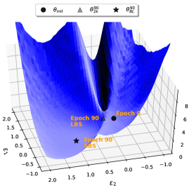
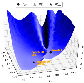
Figure 1: (Left) 3D parametric plot for C1 model on Cifar-10. Points are labeled with the number of epochs (e.g., 90) and the technique that was used to arrive at that point (e.g., large batch size, LBS). The $\epsilon_{1}$ direction shows how the loss changes across the path between initial model at epoch 0, and the final model achieved with Large Batch Size (LBS) of $B=2K$. Similarly, the $\epsilon_{2}$ direction computes the loss when the model parameters are interpolated between epoch 0 and final model at epoch 90 with Small Batch Size (SBS). Note the sharp curvature directions to which LBS gets attracted. (Right) A similar plot, except that we use the ABSA algorithm with final batch of $16K$, rather than SGD with a small batch size for interpolating the $\epsilon_{2}$ direction. Note the visual similarity between the point to which ABSA converges after 90 epochs (ABSA, 84.24% accuracy) and the point to which small batch SGD (SBS, 83.05% accuracy) converges after 90 epochs. Note also that both avoid the sharp landscape to which large batch gets attracted (LBS, 76.82%). Generalization errors are shown in Tab. IV.

Finding the right neural network (NN) model architecture for a particular application typically requires extensive hyper-parameter tuning and architecture search, often on a very large dataset. These delays associated with training NNs are routinely the main bottleneck in the design process. One way to address this issue is to use large distributed processor clusters to perform distributed Stochastic Gradient Descent (SGD). However, to efficiently utilize each processor, the portion of the batch associated with each processor (sometimes called the mini-batch size) must grow correspondingly. In the ideal case, the goal is to decrease the computational time proportional to the increase in batch size, without any drop in generalization quality. However, large batch training has a number of well known drawbacks [15, 31, 39]. These include degradation of accuracy, poor generalization, wasted computation, and even poor robustness to adversarial perturbations [23, 46].

In order to address these drawbacks, many solutions have been proposed [17, 49, 11, 41, 22]. However, these methods either work only for particular models on a particular dataset, or they require extensive hyper-parameter tuning [26, 15, 39]. The latter point is often not discussed in the presentation of record-breaking training-times with large batch sizes. However, these cost are important for a practitioner who wants to accelerate training time with large batches to develop and use a model.

One recent solution is to incorporate adaptive batch size training [41, 11]. The proposed method involves a hybrid increase of batch size and learning rate to accelerate training. In this approach, one would select a strategy to “anneal” the batch size during training. This is based on the idea that large batches contain less “noise,” and that could be used in much the same way as reducing the learning rate during training or the temperature parameter in simulated annealing optimization.

As the use of adaptive batch sizes results in the elastic use of distributed computing resources, this approach is ideally suited to the emerging “pay as you use” era of Serverless Computing [2]. However, there are two major limitations with this approach. First, there is no framework that supports changing of batch size during training and rescaling of the processes. Currently the only approach is to run the problem with a fixed batch size, snapshot the training, and restart a new job with more processes. Second, the training is started with small batches, which can only be scaled to a small number of processes. A simple application of Amdahl’s law shows that the speed up bottleneck will be the portion of the training that uses small batch since it cannot be parallelized to large number of processes.

In this paper, we develop methods to address both of these shortcomings. In more detail, our main contributions are the following.

• We propose an Adaptive Batch Size (ABS) method for SGD training that is based on second order information (i.e., Hessian information). Our method automatically changes the batch size and learning rate based on the loss landscape curvature, as measured via the Hessian spectrum.

• We propose an Adaptive Batch Size Adversarial (ABSA) method for SGD training. This method extends ABS by using an implicit regularization approach based on robust training by solving a min-max optimization problem. In particular, we combine the second order ABS method with recent results of [46] which show that robust training can be used to regularize against sharp minima. We show that this combination of Hessian-based adaptive batch size and robust optimization achieves significantly better test performance (up to 1%; see Table V in Appendix) with little computational overhead.

• We extensively test our proposed solution on a wide range of datasets (Cifar-10/100, SVHN, TinyImageNet, and ImageNet), using different NNs, including residual networks. Importantly, we use the same hyper-parameters for all of the experiments, and we do not perform any kind of tuning to tailor our results. The empirical results show the clear benefit of our proposed method, as compared to the state-of-the-art. The proposed algorithm achieves equal or better test accuracy (up to 1%) and requires significantly fewer SGD updates (up to $5\times$). In addition, if we permit ourselves to perform a slight hyper-parameter tuning of the warmup schedule, then we show that the number of SGD updates can be reduced $44.8\times$ on Cifar-10 and $28.8\times$ on ImageNet.

• We develop a scalable adaptive batch size framework based on Ray [34]. Our framework supports elastic resizing of the cluster to increase or decrease the number of processes. It also supports the adversarial / second order based methods proposed above as well as the adaptive batch size method of [41]. We present the scaling of our proposed method on Amazon Web Services for training ResNet18 on ImageNet, showing negligible cluster resizing cost (0.32% out of entire training time).

While a number of recent works have discussed adaptive batch size or increasing batch size during training [11, 41, 12, 3], to the best of our knowledge this is the first paper to introduce a scalable framework that automatically resizes the batch size and cluster. Moreover, to the best of our knowledge, this is the first work that introduces Hessian information and adversarial training in adaptive batch size training, with extensive testing on many datasets.

Limitations

We believe that it is important for every work to state its limitations (in general, but in particular in this area). We were particularly careful to perform extensive experiments, and we repeated all the reported tests multiple times. We test the algorithm on models ranging from a few layers to hundreds of layers, including residual networks as well as smaller networks such as SqueezeNext. We have also open sourced our code to allow reproducibility [20]. An important limitation is that second order methods have additional overhead for backpropagating the Hessian. Currently, most of the existing frameworks do not support (memory) efficient backpropagation of the Hessian (thus providing a structural bias against these powerful methods). However, the complexity of each Hessian matvec is the same as that for a gradient computation [45, 28]. Our method requires an estimate of the Hessian spectrum, which typically needs ten Hessian matvecs (for power method iterations to reach a relative tolerance of 1e-2). Thus, while the additional cost is not too large, the benefits that we show in terms of testing accuracy and reduced number of updates do come at additional cost (see section IV-D for details). We support this by showing measured Hessian overhead time for an actual training problem as shown in Fig. 4.

II Related Work

Optimization methods based on SGD are currently the most effective techniques for training NNs, and this is commonly attributed to SGD’s ability to escape saddle-points and “bad” local minima [9]. However, the sequential nature of weight updates in synchronous SGD limits possibilities for parallel computing. In recent years, there has been considerable effort on breaking this sequential nature, through asynchronous methods [51] or symbolic execution techniques [27]. A main problem with asynchronous methods is reproducibility, which, in this case, depends on the number of processes used [52, 1]. Due to this issue, recently there have been attempts to increase parallelization opportunities in synchronous SGD by using large batch size training. With large batches, it is possible to distribute computations more efficiently to parallel compute nodes [13], thus reducing the total training time. However, large batch training often leads to sub-optimal test performance [23, 46]. This has been attributed to the observation that large batch size training tends to get attracted to local minima or sharp curvature directions, which are not robust to (possible) mismatch between training and testing curves [23]. A full understanding of this, however, remains elusive (but recent work has used random matrix theory to characterize models trained with smaller or larger batch sizes in terms of stronger or weaker implicit regularization [29, 30]).

Input: Learning rate $\eta$, decay epoch $E_{decay}$, decay ratio $\rho_{lr,decay}$; initial batch $B_{init}$, maximum batch $B_{max}$; Eigenvalue decay ratio $\alpha$, batch/lr increasing ratio $\beta$, duration factor $\kappa$; adversarial input ratio $\gamma$, adversarial magnitude $\epsilon_{adv}$, adversarial input ratio decay factor $\omega$, terminate epoch $\tau$; input data $x$.

Result: Final model parameters $\theta$

Initialize old (new) eigenvalue as $\lambda_{old}$ ($\lambda_{new}$), batch size $B_{itr}$, learning rate $\eta_{itr}$, duration time $\kappa_{itr}=0$.

for Epoch $=1,2,3\ldots$ do

       for $t=1,2,3\ldots$ do // mini-batch iterations

             generate adversarial data $x_{adv}$ by the ratio of $\gamma$;

            SGD update;

      compute $\lambda_{new}$; // Hessian power-iteration

      $\kappa_{itr}\mathrel{+}=1$;

      $Flag=\{(\lambda_{new}<\lambda_{old}/\alpha)~{}OR~{}(\kappa_{itr}=\kappa)\}$;

      if Flag then // adaptively change batch/lr

             $B_{itr}\mathrel{*}=\beta$;   $\eta_{itr}\mathrel{*}=\beta$; $\gamma\mathrel{/}=\omega$;  $\kappa_{itr}=0$; 

      if $\lambda_{new}<\lambda_{old}/\alpha$ then

             $\lambda_{old}=\lambda_{new}$;

      if Epoch $=\tau$  then

             $\gamma=0$;

      if Epoch in $E_{decay}$ then // lr decay schedule

             $\eta_{itr}\mathrel{/}=\rho_{lr,decay}$ ;

Algorithm 1 Adaptive Batch Size (ABS) and Adaptive Batch Size Adversarial (ABSA)

There have been several solutions proposed for alleviating the problem with large batch size training. The first notable work here is [17], where it was shown that by scaling the learning rate, it is possible to achieve the same testing accuracy for large batches. In particular, ResNet50 model was tested on ImageNet dataset, and it was shown that the baseline accuracy could be recovered up to batch size of 8192. However, this approach does not generalize to other networks/tasks [15]. In [49], an adaptive learning rate method was proposed which allowed scaling training to a much larger batch size of 32K with more hyper-parameter tuning. More recent work [22] proposed mix-precision method to explore further the limit of large batch training. There is also a set of work on dynamic batch size selection to accelerate optimization, where the batch size is selected to ensure a search direction that would decrease the loss function with high probability [5, 7, 4]. Another notable work is the use of distributed K-FAC method to perform large batch training [36].

Work has also focused on using second order methods to reduce the brittleness of SGD. Most notably, [37, 44] show that Newton/quasi-Newton methods outperform SGD for training NNs. However, their results only consider simple fully-connected NNs and auto-encoders. A problem with naive second-order methods is that they can exacerbate the large batch problem, as by construction they have a higher tendency to get attracted to local minima, as compared to SGD. For these reasons, early attempts at using second-order methods for training convolutional NNs have so far not been successful.

A recent study has shown that anisotropic noise injection based on second order information could also help in escaping sharp landscape [53]. The authors showed that the noise from SGD could be viewed as anisotropic, with the Hessian as its covariance matrix. Injecting random noise using the Hessian as covariance was proposed as a method to avoid sharp landscape points.

Another recent work by [46] has shown that adversarial training (or robust optimization) could be used to “regularize” against these sharp minima, with preliminary results showing superior testing performance, as compared to other methods. In addition, [38, 40] used adversarial training and showed that the model trained using robust optimization is often more robust to perturbations, as compared to normal SGD training. Similar observations have been made by others [16]. These works are in line with recent results showing that adversarial attacks can sometimes be interpreted as providing useful features [21].

Our results are in agreement with recent studies showing that there is a limit beyond which increasing batch size will lead to diminishing results [15, 26, 39]. These studies mainly focus on constant batch size. However, the work of  [15] showed that warmup with smaller batches can noticeably delay this limit to larger batches. An adaptive batch size strategy would involve several different batches throughout the training, and this adaptive schedule would be more efficient in the regime of large batches [31]. This means that increasing the batch size in each segment of this adaptive schedule would be more efficient in terms of minimum number of optimization steps [31]. Our goal is to achieve this using ABS/ABSA algorithms to fully exploit larger batches during training, and delay the limit beyond which using large batches would result in diminishing returns.

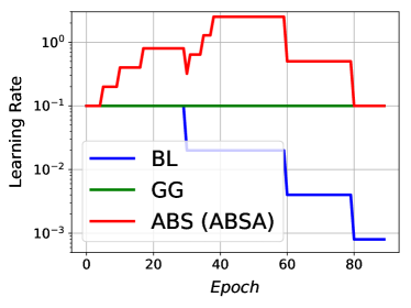
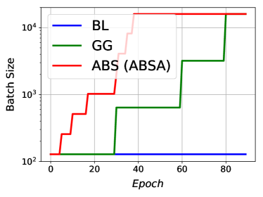
Figure 2: Illustration of learning rate (left) and batch size (right) schedules of adaptive batch size, as a function of training epochs using C2 (Wide-ResNet) model on Cifar-10.

TABLE I: Accuracy and number of parameter updates of C3 (SqueezeNext) on Cifar-10.

	BL		FB		GG		ABS		ABSA
BS	Acc.	# Iters	Acc.	# Iters	Acc.	# Iters	Acc.	# Iters	Acc.	# Iters
128	92.02	78125	N.A.	N.A.	N.A.	N.A.	N.A.	N.A.	N.A.	N.A.
256	91.88	39062	91.75	39062	91.84	50700	91.7	40792	92.11	43352
512	91.68	19531	91.67	19531	91.19	37050	92.15	32428	91.61	25388
1024	89.44	9766	91.23	9766	91.12	31980	91.61	17046	91.66	23446
2048	83.17	4882	90.44	4882	89.19	30030	91.57	21579	91.61	14027
4096	73.74	2441	86.12	2441	91.83	29191	91.91	18293	92.07	21909
8192	63.71	1220	64.91	1220	91.51	28947	91.77	22802	91.81	16778
16384	47.84	610	32.57	610	90.19	28828	92.12	17485	91.97	24361

III Method

We consider a supervised learning framework where the goal is to minimize a loss function $L(\theta)$:

$$L(\theta)=\frac{1}{N}\sum_{i=1}^{N}l(z_{i},\theta),$$ (1)

where $\theta$ are the model weight parameters, $Z=(X,Y)$ is the training dataset, and $l(z,\theta)$ is the loss for a datum $z\in Z$. Here, $X$ is the input, $Y$ is the corresponding label, and $N=|Z|$ is the cardinality of the training set. SGD is typically used to optimize Eq. (1) by taking steps of the form:

$$\theta_{t+1}=\theta_{t}-\eta_{t}\frac{1}{|B|}\sum_{z\in B}\nabla_{\theta}l(z,\theta_{t}),$$ (2)

where $B$ is a mini-batch of examples drawn randomly from $Z$, and $\eta_{t}$ is the step size (learning rate) at iteration $t$. In the case of large batch size training, the batch size is increased to large values.

As mentioned above, large batch size training often results in convergence to a point with “sharp” curvature that often exhibits poor generalization. To clearly illustrate this, we show a 3D parametric plot of the loss landscape when interpolating between the model parameters in the beginning of training (Epoch 0) and at the end of training (Epoch 90) with large batch size for the first direction, and interpolate between the same initialization and weights of the model trained with small batch at Epoch 90. We compute this plot for multiple different models and networks (see Fig. 1, 9 and 10). One can clearly see that the large batch experiments get attracted to a sharper landscape point, whereas the small batch training ends in a significantly flatter point. One popular rationalization of this is that small batch training has sufficient noise to escape such sharp landscape points.

III-A Adaptive Batch Size (ABS) and Adaptive Batch Size Adversarial (ABSA) based on Hessian Information and Adversarial Training

To address the above problem, [42] proposed an adaptive batch size scheme which controls SGD noise by increasing batch size instead of adjusting the learning rate. The adaptive batch size method proposed by [41] is shown in Fig. 2. While this method performs very well, its overall speed up is bottlenecked by the small batch size, which is used for 30 epochs. (Based on Amdahl’s law, even if the rest of the 60 epochs is trained with infinite speed, the overall training time will be bounded by the first 30 epochs.) The effect of this bottleneck could be reduced, if we could increase the batch size sooner. This could be done by manual tuning of the batch size schedule, but as mentioned before manual tuning is not desired due to additional overhead for the practitioner.

To address this, we incorporate second-order information to determine when the batch size could be increased. The corresponding schedule is shown in red in Fig. 2. The main intuition is to use small batch sizes when the loss landscape has sharper curvature and to use large batch sizes when the loss landscape has flatter curvature. That is, we aim to keep the SGD noise high to escape the sharp landscape shown in Fig. 1. To this end, a smaller batch size is used in regions with a “sharper” loss landscape to help avoid attraction to landscape points with poor generalization. We then switch to a larger batch size only in regions where the loss has a “flatter” landscape. As in the hybrid method of [42], we also scale the learning rate proportional to batch size increasing ratio to maintain the noise level.

However, a key problem here is measuring the loss landscape’s curvature. Naively forming the Hessian operator has a prohibitive computational cost. However, we can efficiently compute the top eigenvalues of the Hessian operator using power method, using a matrix free algorithm. Let us denote the gradient of $L(\theta)$ w.r.t. $\theta$ by $g$. Then, for a random vector, whose dimension is the same as $g$, we have:

$$\frac{\partial(g^{T}v)}{\partial\theta}=\frac{\partial g^{T}}{\partial\theta}v+g^{T}\frac{\partial v}{\partial\theta}=\frac{\partial g^{T}}{\partial\theta}v=Hv,$$ (3)

where $H$ is Hessian matrix. Here, the second equation comes from the fact that $v$ is independent to $\theta$. We have developed an efficient implementation to compute curvature information by using the same automatic differentiation pipeline that is used for backpropagating the gradient [20]. The algorithm is shown in Alg. 2. The power iteration algorithm starts with a vector drawn randomly from a Gaussian distribution, followed by successive application of the Hessian operator to this vector (so called ‘matvec’). Thus, instead of computing the full Hessian matrix we simply backpropagate this matvec.

Input: Parameter: $\theta$.

Compute the gradient of $\theta$ by backpropagation, i.e., $g=\frac{dL}{d\theta}$.

Draw a random vector $v$ (same dimension as $\theta$).

Normalize $v$, $v=\frac{v}{\|v\|_{2}}$

for i $=1,2,\ldots,n$ do        // Power Iteration

       Compute $gv=g^{T}v$

        // Inner product

      

      Compute $Hv$ by backpropagation, $Hv=\frac{d(gv)}{d\theta}$

        // Get Hessian vector product

      

      Normalize and reset $v$, $v=\frac{Hv}{\|Hv\|_{2}}$

Algorithm 2 Power Iteration for Eigenvalue Computation

In our approach, the Hessian spectrum is only calculated at the end of every epoch, and thus it has small computational overhead. We increase the batch size in proportion to how much the Hessian spectrum decays, as compared to the curvature at initialization The pseudo-code for this ABS algorithm is shown in Alg. 1.

The second component of our framework is robust optimization. In [46], the authors empirically showed that adversarial training leads to more robust models with respect to adversarial perturbation. An interesting corollary was that, with adversarial training, the model converges to regions that are considerably flatter, as compared to the normal SGD training. Therefore, we use adversarial training as a regularization term to help regularize against sharp landscape. Our empirical results have consistently shown improved results. We refer to this as the Adaptive Batch Size with Adversarial (ABSA) method; see Alg. 1 for the ABSA pseudo-code. In ABSA, we solve a min-max problem instead of a normal empirical risk minimization problem [23, 46]:

$$\min_{\theta}\max_{\Delta x\in\mathcal{U}}L(x,y;\theta),$$ (4)

where $\mathcal{U}$ is an admissibility set for acceptable perturbations (typically restricting the magnitude of the perturbation). Solving this min-max problem for NNs is an intractable problem, and thus we approximately solve the maximization part through the Fast Gradient Sign Method (FGSM), proposed by [16]. This basically corresponds to generating adversarial inputs using one gradient ascent step (i.e., the perturbation is computed by $\Delta x=\epsilon\operatorname{sign}(\nabla_{x}l(x,y;\theta))$). Other possible choices are proposed by [43, 8, 33, 47].

Fig. 2 illustrates our ABS/ABSA schedule as compared to a normal training strategy and the adaptive batch size method of [41, 11]. As we show in section IV, our combined approach (second order and robust optimization) not only achieves better accuracy, but it also requires significantly fewer SGD updates, as compared to [41, 11].

III-B Distributed Elastic Training

Efficient adaptive batch size training is a unique workload that is not well-supported by existing deep learning and cluster computing frameworks. As the batch size increases, more GPUs can be used to parallelize and accelerate the workload. However, all existing solutions for synchronous distributed training assumes a static allocation of GPU resources specified at the beginning of training, while efficient adaptive batch size training forces the resource allocation to be dynamic. Furthermore, though cluster computing offerings such as Kubernetes and AWS offer autoscaling functionality for elastic resource provisioning, there is no existing framework that tightly couples this autoscaling with the SGD training. To address this, we develop an execution framework for efficient resource-elastic training. We build our framework upon Ray [34], a distributed execution engine that provides a distributed training interface and a resource requesting API for increasing the size of the cluster. This framework enables efficient GPU allocation from the cloud provider, enabling us to resize training as the target batch size becomes larger. We use PyTorch for the underlying distributed SGD and Hessian based computations. Our distributed Hessian-based computation implements a distributed power iteration, where each process computes Hessian matvec on a subset of input data, and the result is accumulated through an all-reduce collective.

IV Results

We evaluate the performance of ABS/ABSA on different datasets (ranging from O(1E5) to O(1E7) training examples) and multiple NN models. We compare the baseline SGD performance, along with other state-of-the-art methods proposed for large batch training [41, 17]. Notice that GG [41] and ABS/ABSA have different batch sizes during training. Hence the batch size reported in our results represents the maximum batch size during training. To allow for a direct comparison we also report the number of weight updates in our results (lower is better). We also report the computed wall-clock time as well using our Ray based framework for adaptive batch size implementation.

Preferably we would want a higher testing accuracy along with fewer SGD updates. Unless otherwise noted, we do not change any of the hyper-parameters for ABS/ABSA. We use the exact same parameters used in the baseline model, and we do not tailor any parameters to suit our algorithm. A detailed explanation of the different NN models, and the datasets is given in Appendix B.

Section IV-A shows the result of ABS/ABSA compared to BaseLine (BL), FB [17] and GG [41]. Section IV-B presents the results on more challenging datasets of TinyImageNet and ImageNet. In section IV-C, we show with slight hyper-parameter tuning on warm-up phase, ABSA can achieve better results. Finally, we report the real wall-clock time training by our distribution framework on AWS in section IV-D.

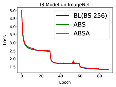
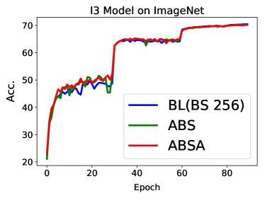
Figure 3: I3 (ResNet18) model on ImageNet. Training set loss (left) and testing set accuracy (right), evaluated as a function of epochs.

IV-A ABS and ABSA for SVHN and Cifar

Tab. I and Tab. III-VII report the test accuracy and the number of parameter updates for different datasets and models (see Appendix D for Tab. III-VII). First, note the drop in BL accuracy for large batch, confirming the accuracy degradation problem. Moreover, note that the FB strategy only works well for moderate batch sizes (it diverges for large batch). However, the GG method has a very consistent performance, but its number of parameter updates is usually greater than our method. Looking at the last two major columns of Tab. I and Tab. III-VII, the test performance that ABS achieves is similar to BL. Overall, the number of updates of ABS is 3-10 times smaller than BL with batch size 128. Also, note that for most cases ABSA achieves superior accuracy. This confirms the effectiveness of adversarial training combined with the second order information. Furthermore, we show a similar 3D parametric plot for ABSA algorithm in Fig. 1, 9 and 10. Note that ABSA avoids the sharp landscape of large batch and is able to converge to a landscape with similar curvature as that of BL with small batch training.

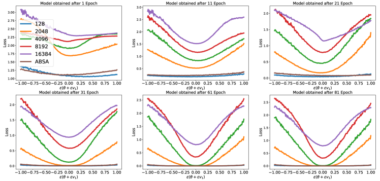
Figure 11: The landscape of the loss is shown when the model parameters are perturbed along the dominant Hessian eigenvector, $v_{1}$, for C1 on Cifar-10 dataset. Here $\epsilon$ is a scalar that perturbs the model parameters along $v_{1}$. The top rows show the landscape for epochs 1, 11, and 21 and the bottom row shows epochs 31, 61, and 81. One can clearly see, that larger batches continuously get stuck/attracted in areas with larger curvature whereas small batch SGD or ABSA (with batch of 16K) can escape such landscape. For detailed generalization error please see Tab. IV.

Furthermore, we show the loss landscape of model obtained throughout the training process along the dominant eigenvalue [46] in Fig. 11 in Appendix D. It can be clearly seen that throughout training larger batches tend to get stuck/attracted to areas with larger curvature, while small batch SGD and ABSA are able to avoid them.

IV-B ABSA for TinyImageNet and ImageNet

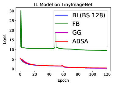
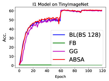
Figure 7: I1 model on TinyImageNet. Training set loss (left), and testing set accuracy (right), evaluated as a function of epochs. All results correspond to batch size 16384 (please see Tab. VIII for details). As one can see, from epoch 60 to 80, the test performance drops due to overfitting. However, ABSA achieves the best performance with apparently less overfitting (it has higher training loss).

Here, we report the ABSA method on more challenging datasets, specifically, TinyImageNet and ImageNet. We use the exact same hyper-parameters in our algorithm as for Cifar/SVHN, even though tuning them could potentially be preferable for us. All TinyImageNet results are in the Appendix D; see Fig. 7 and Tab. VIII.

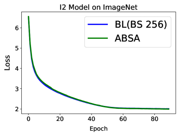
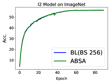
Figure 8: I2 model on ImageNet. Training set loss (a), and testing set accuracy (b), evaluated as a function of epochs.

Due to the limited computational resources, we only test ABSA and BL (baseline with small batch) for ImageNet, and we report results in Fig. 8 (see Appendix D). We first start with I2 model (AlexNet) whose baseline requires $450K$ parameter updates (i.e., SGD iterations), reaching $56.32\%$ validation accuracy. For ABSA, the final validation accuracy is $56.40\%$, with only $76K$ parameter updates. The maximum batch size reached by ABSA is $16,384$, with initial batch size $256$.

We also test I3 (ResNet18) model on ImageNet, as shown in Fig. 3. The BL with batch of 256 reaches $70.46\%$ validation accuracy with $450K$ parameter updates. The final validation accuracies of ABS and ABSA are $70.15\%$ and $70.24\%$, respectively, both with $66,393$ parameter updates. The maximum batch size reached by ABS and ABSA is $16,384$ with initial batch size $256$. If GG schedule is implemented, the total number of parameter updates would have been $166K$. (Due to the limitation of resource, we do not run GG.)

IV-C ABSA with Warm-up Tuning

To effectively speed up training, large batch should not require extensive hyper-parameter tuning. However, a recent trend (mainly motivated by industry labs) is focused on showing how fast training on a benchmark task could be finished on a supercomputer  [49, 32, 48, 17, 42]. This is mostly not possible with academic resources. However, to illustrate how ABSA’s performance could be boosted by additional hyper-parameter tuning, we solely focus on the warmup schedule (and keep all the other hyper-parameters such as $\alpha,~{}\beta$ the same). For the warmup tuning, our goal is to ramp up to large batches quickly. On Cifar-10 with C1 model, we increase the initial batch size to $1920$ (as compared to baseline batch size $128$), and we gradually increase the learning rate in five epochs, as in [17]. The final accuracy of this mixed schedule is 83.24% with 784 SGD updates (compared to 83.04% for baseline with $35K$ SGD updates, which is $48.1\times$ smaller).

On ImageNet with I3 model, we increase the initial batch size to $4096$ (as compared to baseline batch size $256$) with largest batch size $16K$, and we gradually increase the learning rate in 20 epochs, and train for a total of 100 epochs. The final accuracy is $70.04\%$ with $14.8K$ SGD updates (as compared to 70.4% for baseline with 450k SGD updates, which is $28.8\times$ smaller).

We emphasize that these results are achieved with moderate hyper-parameter tuning though only 10 trials; and also we did not tune any other hyper-parameters introduced by ABSA. It is quite feasible that with an industrial infrastructure and tuning of learning rate, momentum, and ABSA’s parameters, the results could significantly be improved.

IV-D Training Time Measurement

To show the scaling of our framework, we test both GG and ABSA for ResNet18 ImageNet training. We set the batch size per GPU to be 256 and run our experiments on AWS EC2 using p3.16xlarge instances. We report SGD computation/communication, cost of resizing the cluster, and Hessian computation time, as shown in Fig. 4 and Tab. II. We see that resizing and communication time only introduce slight overhead to computation time. GG only reduces the training time from 125K to 51K seconds because it is bottlenecked by the first phase with 256 batch size, as shown in Fig. 2. ABSA further reduces the training time to 29.4K seconds. Note that the Hessian spectrum computation only accounts for 9.3% of the entire training time. The main bottleneck of ABSA Hessian computation is that at the very beginning, we only allow 1 or 2 GPUs to compute Hessian information, which has to be done with gradient accumulation. For ABSA Tuned, where we tune the warm-up phase, the time can be reduced to 14.2K. Again, note the small overhead of the Hessian computation, as compared to the total training time.

Figure 4: Breakdown of the different methods’ runtimes for our Ray based adaptive batch size framework. In particular, note the very small overhead for resizing the cluster, as well as the small Hessian computation overhead for ABSA.

Method	Comp	Comm	Resize	Hess	Total	Speedup
Baseline	125073	N/A	N/A	N/A	125073	1x
GG	50965	54	40	N/A	51059	2.45x
ABSA	26404	230	95	2746	29475	4.24x
ABSA Tuned	13935	58	39	220	14252	8.78x

TABLE II: Breakdown of ResNet18 training time on ImageNet for GG [42], ABSA, and ABSA Tuned. For the latter, we only tuned the warm-up phase and did not tune any other hyper-parameters. We report SGD computation time (Comp), SGD communication time (Comm), cost of resizing the cluster (Resize), overhead of Hessian computation and communication (Hess), and the total training time (Total) to reach baseline accuracy.

V Conclusion

In this work, we address two major challenges for adaptive batch size training of NNs. First, we developed a new framework based on Ray that allows efficient dynamic scaling of the cluster with negligible resize cost. Even so, the speed up of existing adaptive batch size methods is limited by the initial portion of the training with small batch size. Thus, we presented a Hessian based method which allows more rapid increase of the batch size during the initial phase. This reduces the impact of this phase on overall speed up. We extensively test these and other related methods on five datasets with multiple NN models (AlexNet, ResNet, Wide ResNet and SqueezeNext). To do so, we performed two sets of experiments, one without any hyper-parameter tuning, and one where we only tuned the warm-up phase of the training. In both cases, our ABSA method enables one to increase batch size more rapidly resulting in fewer number of SGD iterations. Furthermore, we showed scaling results of our proposed method and measured run times on AWS for both pior work [41] as well as our ABSA method. To enable reproducibility, we open source our distribution tools in [20].

Appendix A Convergence Rate of ABS

Here, we provide a straightforward proof that ABS algorithm does converge for strongly convex problems. This proof is a basic modification of SGD’s convergence proof with constant batch size. Based on an assumption about the loss (Assumption 2 in Appendix A-A), it is not hard to prove the following theorem.

Theorem 1.

Under Assumption 2, assume at step $t$, the batch size used for parameter update is $b_{t}$, the step size is $b_{t}\eta_{0}$, where $\eta_{0}$ is fixed and satisfies,

$$0<\eta_{0}\leq\frac{1}{L_{g}(M_{v}+B_{\max})},$$ (5)

where $B_{\max}$ is the maximum batch size during training. Then, with $\theta_{0}$ as the initialization, the expected optimality gap satisfies the following inequality,

$$\mathbb{E}[L(\theta_{t+1})]-L_{*}\leq\prod_{k=1}^{t}(1-b_{k}\eta_{0}c_{s})(L(\theta_{0})-L_{*}-\frac{\eta_{0}L_{g}M}{2c_{s}})+\frac{\eta_{0}L_{g}M}{2c_{s}}.$$ (6)

From Theorem 1, if $b_{t}\equiv 1$, the convergence rate for $t$ steps, based on equation 6, is $(1-\eta_{0}c_{s})$. However, the convergence rate of Alg. 1 becomes $\prod_{k=1}^{t}(1-b_{k}\eta_{0}c_{s})$, where $1\leq b_{k}\leq B_{max}$. With an adaptive $b_{t}$ Alg. 1 can converge faster than basic SGD. We show empirical results for a logistic regression problem in the Appendix A-A, which is a simple convex problem.

A-A Proof of Theorem

For a finite sum objective function $L(\theta)$, i.e., equation 1, we assume that:

Assumption 2.

The objective function $L(\theta)$ satisfies:

• $L(\theta)$ is continuously differentiable and the gradient function of $L$ is Lipschitz continuous with Lipschitz constant $L_{g}$, i.e.

  $$\|\nabla L(\theta_{1})-\nabla L(\theta_{2})\|\leq L_{g}\|\theta_{1}-\theta_{2}\|,~{}~{}~{}~{}~{}~{}~{}~{}~{}~{}\text{for all $\theta_{1}$ and $\theta_{2}$}.$$ (7)

• $L(\theta)$ is strongly convex, i.e., there exists a constant $c_{s}>0$ s.t.

  $$L(\theta_{2})\geq L(\theta_{1})+\nabla L(\theta_{1})^{T}(\theta_{2}-\theta_{1})+\frac{1}{2}c_{s}\|\theta_{1}-\theta_{2}\|^{2},~{}~{}~{}~{}~{}~{}~{}~{}~{}~{}\text{for all $\theta_{1}$ and $\theta_{2}$}.$$ (8)

  Also, the global minima of $L(\theta)$ is achieved at $\theta_{*}$ and $L(\theta_{*})=L_{*}$.

• Each gradient of each individual $l_{i}(z_{i})$ is an unbiased estimation of the true gradient, i.e.

  $$\mathbb{E}[\nabla l_{i}(z_{i},\theta)]=\nabla L(\theta),~{}~{}~{}~{}~{}~{}~{}~{}~{}~{}\text{for all $i$}.$$ (9)

• There exist scalars $M\geq 0$ and $M_{v}\geq 0$ s.t.

  $${\mathbb{V}}(\nabla l_{i}(z_{i},\theta))\leq M+M_{v}\|\nabla L(\theta)\|,~{}~{}~{}~{}~{}~{}~{}~{}~{}~{}\text{for all $i$},$$ (10)

  where ${\mathbb{V}}(\cdot)$ is the variance operator, i.e.

  $${\mathbb{V}}(\nabla l_{i}(z_{i},\theta))=\mathbb{E}[\|\nabla l_{i}(z_{i},\theta)\|^{2}]-\|\mathbb{E}[\nabla l_{i}(z_{i},\theta)]\|^{2}.$$

From the Assumption 2, it is not hard to get,

$$\mathbb{E}[\|\nabla l_{i}(z_{i},\theta)\|^{2}]\leq M+M_{g}\|\nabla L(\theta)\|^{2},$$ (11)

with $M_{g}=M_{v}+1$.

With Assumption 2, the following two lemmas could be found in any optimization reference, e.g. [6]. We give the proofs here for completeness.

Lemma 3.

Under Assumption 2, after one iteration of stochastic gradient update with step size $\eta_{t}$ at $\theta_{t}$, we have

$$\mathbb{E}[L(\theta_{t+1})]-L(\theta_{t})\leq-(1-\frac{1}{2}\eta_{t}L_{g}M_{g})\eta_{t}\|\nabla L(\theta_{t})\|^{2}+\frac{1}{2}\eta_{t}^{2}L_{g}M,$$ (12)

where $\theta_{t+1}=\theta_{t}-\eta_{t}\nabla l_{i}(\theta,z_{i})$ for some $i$.

Proof.

With the $L_{g}$ smooth of $L(\theta)$, we have

$$\mathbb{E}[L(\theta_{t+1})]-L(\theta_{t}) \leq-\eta_{t}\nabla L(\theta_{t})\mathbb{E}[\nabla l_{i}(\theta,z_{i})]+\frac{1}{2}\eta_{t}^{2}L_{g}\mathbb{E}[\|\nabla l_{i}(\theta,z_{i})\|^{2}]$$

$$\leq-\eta_{t}\|\nabla L(\theta_{t})\|^{2}+\frac{1}{2}\eta_{t}^{2}L_{g}(M+M_{g}\|\nabla L(\theta_{t})\|^{2}).$$

From above, the result follows. ∎

Lemma 4.

Under Assumption 2, for any $\theta$, we have

$$2c_{s}(L(\theta)-L_{*})\leq\|\nabla L(\theta)\|^{2}.$$ (13)

Proof.

Let

$$h(\bar{\theta})=L(\theta)+\nabla L(\theta)^{T}(\bar{\theta}-\theta)+\frac{1}{2}c_{s}\|\bar{\theta}-\theta\|^{2}.$$

Then $h(\bar{\theta})$ has a unique global minima at $\bar{\theta}_{*}=\theta-\frac{1}{c_{s}}\nabla L(\theta)$ with $h(\bar{\theta}_{*})=L(\theta)-\frac{1}{2c_{s}}\|\nabla L(\theta)\|^{2}$. Using the strong convexity of $L(\theta)$, it follows

$$L(\theta_{*})\geq L(\theta)+\nabla L(\theta)^{T}(\theta_{*}-\theta)+\frac{1}{2}c_{s}\|\theta-\theta_{*}\|_{2}^{2}=h(\bar{\theta}_{*})=L(\theta)-\frac{1}{2c_{s}}\|\nabla L(\theta)\|^{2}.$$

∎

The following lemma is trivial, we omit the proof here.

Lemma 5.

Let $L_{B}(\theta)=\frac{1}{|B|}\sum_{z_{i}\in B}l_{i}(\theta,z_{i})$. Then the variance of $\nabla L_{B}(\theta)$ is bounded by

$${\mathbb{V}}(\nabla L_{B}(\theta))\leq M/|B|+M_{v}\|\nabla L(\theta)\|/|B|,~{}~{}~{}~{}~{}~{}~{}~{}~{}~{}\text{for all B}.$$ (14)

Proof of Theorem 1

Given these lemmas, we now proceed with the proof of Theorem 1.

Proof.

Assume the batch used at step t is $b_{t}$, according to Lemma 3 and 5,

$$\mathbb{E}[L(\theta_{t+1})]-L(\theta_{t}) \leq-(1-\frac{1}{2}b_{t}\eta_{0}L_{g}(\frac{M_{v}}{b_{t}}+1))b_{t}\eta_{0}\|\nabla L(\theta_{t})\|^{2}+\frac{1}{2}(b_{t}\eta_{0})^{2}L_{g}\frac{M}{b_{t}}$$

$$\leq-(1-\frac{1}{2}\eta_{0}L_{g}(M_{v}+b_{t}))b_{t}\eta_{0}\|\nabla L(\theta_{t})\|^{2}+\frac{1}{2}b_{t}\eta_{0}^{2}L_{g}M$$

$$\leq-(1-\frac{1}{2}\eta_{0}L_{g}(M_{v}+B_{\max}))b_{t}\eta_{0}\|\nabla L(\theta_{t})\|^{2}+\frac{1}{2}b_{t}\eta_{0}^{2}L_{g}M$$

$$\leq-\frac{1}{2}b_{t}\eta_{0}\|\nabla L(\theta_{t})\|^{2}+\frac{1}{2}b_{t}\eta_{0}^{2}L_{g}M$$

$$\leq-b_{t}\eta_{0}c_{s}(L(\theta_{t})-L_{*})+\frac{1}{2}b_{t}\eta_{0}^{2}L_{g}M,$$

where the last inequality is from Lemma 4. This yields

$$\mathbb{E}[L(\theta_{t+1})]-L_{*} \leq L(\theta_{t})-b_{t}\eta_{0}c_{s}(L(\theta_{t})-L_{*})+\frac{1}{2}b_{t}\eta_{0}^{2}L_{g}M-L_{*}$$

$$=(1-b_{t}\eta_{0}c_{s})(L(\theta_{t})-L_{*})+\frac{1}{2}b_{t}\eta_{0}^{2}L_{g}M.$$

It is not hard to see,

$$\mathbb{E}[L(\theta_{t+1})]-L_{*}-\frac{\eta_{0}L_{g}M}{2c_{s}}\leq(1-b_{t}\eta_{0}c_{s})(L(\theta_{t})-L_{*}-\frac{\eta_{0}L_{g}M}{2c_{s}}),$$

from which it follows:

$$\mathbb{E}[L(\theta_{t+1})]-L_{*}-\frac{\eta_{0}L_{g}M}{2c_{s}}\leq\prod_{k=1}^{t}(1-b_{k}\eta_{0}c_{s})(L(\theta_{0})-L_{*}-\frac{\eta_{0}L_{g}M}{2c_{s}}).$$

Therefore,

$$\mathbb{E}[L(\theta_{t+1})]-L_{*}\leq\prod_{k=1}^{t}(1-b_{k}\eta_{0}c_{s})(L(\theta_{0})-L_{*}-\frac{\eta_{0}L_{g}M}{2c_{s}})+\frac{\eta_{0}L_{g}M}{2c_{s}}.$$

∎

We show a toy example of binary logistic regression on mushroom classification dataset. We split the whole dataset to 6905 for training and 1819 for validation. $\eta_{0}=1.2$ for SGD with batch size 100 and full gradient descent. We set $100\leq b_{t}\leq 3200$ for our algorithm, i.e. ABS. Here we mainly focus on the training losses of different optimization algorithms. The results are shown in Figure 5. In order to see if $\eta_{0}$ is not an optimal step size of full gradient descent, we vary $\eta_{0}$ for full gradient descent; see results in Figure 5.

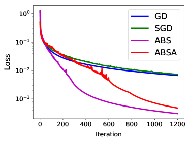
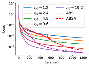
Figure 5: Logistic regression model result. The left figure shows the training loss as a function of iterations for full gradient, SGD, ABS and ABSA. The right figure shows the result of ABS/ABSA compared to full gradient with different learning rate.

Appendix B Training Details

In this section, we give the detailed outline of our training datasets, models, strategy as well as hyper-parameter used in Alg 1.

Dataset. We consider the following datasets.

• SVHN. The original SVHN [35] dataset is small. However, in this paper, we choose the additional dataset, which contains more than 500k samples, as our training dataset.

• Cifar. The two Cifar (i.e., Cifar-10 and Cifar-100) datasets [24] have same number of images but different number of classes.

• TinyImageNet. TinyImageNet consists of a subset of ImangeNet images [10], which contains 200 classes. Each of the class has 500 training and 50 validation images. The size of each image is $64\times 64$.

• ImageNet. The ILSVRC 2012 classification dataset [10] consists of 1000 images classes, with a total of 1.2 million training images and 50,000 validation images. During training, we crop the image to $224\times 224$.

Model Architecture. We implement the following convolution NNs. When we use data augmentation, it is exactly same the standard data augmentation scheme as in the corresponding model.

• S1. AlexNet like model on SVHN as same as [46, C1]. We train it for 20 epochs with initial learning rate $0.01$, and decay a factor of 5 at epoch 5, 10 and 15. There is no data augmentation. The batch size to compute Hessian information is $128$.

• C1. ResNet20 on Cifar-10 dataset [19]. We train it for 90 epochs with initial learning rate $0.1$, and decay a factor of 5 at epoch 30, 60, 80. There is no data augmentation. The batch size to compute Hessian information is $128$.

• C2. Wide-ResNet 16-4 on Cifar-10 dataset [50]. We train it for 90 epochs with initial learning rate $0.1$, and decay a factor of 5 at epoch 30, 60, 80. There is no data augmentation. The batch size to compute Hessian information is $128$.

• C3. SqueezeNext on Cifar-10 dataset [14]. We train it for 200 epochs with initial learning rate $0.1$, and decay a factor of 5 at epoch 60, 120, 160. Data augmentation is implemented. The batch size to compute Hessian information is $128$.

• C4. 2.0-SqueezeNext (twice width) on Cifar-10 dataset [14]. We train it for 200 epochs with initial learning rate $0.1$, and decay a factor of 5 at epoch 60, 120, 160. Data augmentation is implemented.

• C5. ResNet18 on Cifar-100 dataset [19]. We training it for 160 epochs with initial learning rate $0.1$, and decay a factor of 10 at epoch 80, 120. Data augmentation is implemented. The batch size to compute Hessian information is $1024$.

• I1. ResNet50 on TinyImageNet dataset [19]. We training it for 120 epochs with initial learning rate $0.1$, and decay a factor of 10 at epoch 60, 90. Data augmentation is implemented. The batch size to compute Hessian information is $2048$.

• I2. AlexNet on ImageNet dataset [25]. We train it for 90 epochs with initial learning rate $0.01$, and decay it to $0.0001$ quadratically at epoch 60, then keeps it as $0.0001$ for the remaining 30 epochs. Data augmentation is implemented. The batch size to compute Hessian information is $4096$.

• I3. ResNet18 on ImageNet dataset [19]. We train it for 90 epochs with initial learning rate $0.1$, and decay a factor of 10 at epoch 30, 60 and 80. Data augmentation is implemented. The batch size to compute Hessian information is $4096$.

B-A Training Strategy:

We use the following training strategies

• BL. Use the standard training procedure.

• FB. Use linear scaling rule [17] with warm-up stage.

• GG. Use increasing batch size instead of decay learning rate [41].

• ABS. Use our adaptive batch size strategy without adversarial training.

• ABSA. Use our adaptive batch size strategy with adversarial training.

For adversarial training, the adversarial data are generated using Fast Gradient Sign Method (FGSM) [16]. The hyper-parameters in Alg. 1 ($\alpha$ and $\beta$) are chosen to be $2$, $\kappa=10$, $\epsilon_{adv}=0.005$, $\gamma=20\%$, and $\omega=2$ for all the experiments. The only change is that for SVHN, the frequency to compute Hessian information is $65536$ training examples as compared to one epoch, due to the small number of total training epochs (only 20).

Appendix C Approximate Hessian

One of the limitations of second order methods is the additional computational cost for computing the top Hessian eigenvalue. If we use the full Hessian operator, the second backpropagation needs to be done all the way to the first layer of NN. For deep networks this could lead to high computational cost. Here, we empirically explore whether we could use approximate second order information, and in particular we test a block Hessian approximation as illustrated in Fig. 6. The block approximation corresponds to only analyzing the Hessian of the last few layers.

In Fig. 6, we plot the trace of top eigenvalues of full Hessian and block Hessian for C1 model. Although the top eigenvalue of block Hessian has more variance than that of full Hessian, the overall trends are similar for C1. The test performance of C1 on Cifar-10 with block Hessian is $84.82\%$ with 4600 parameter updates (as compared to $84.42\%$ for full Hessian ABSA). The test performance of C4 on Cifar-100 with block Hessian is $68.01\%$ with 12500 parameter updates (as compared to $68.43\%$ for full Hessian ABSA). These results suggest that using a block Hessian to estimate the trend of the full Hessian might be a good choice to overcome computation cost, but a more detailed analysis is needed. Other approaches such as sketching might be another possible direction to reduce this overhead [18].

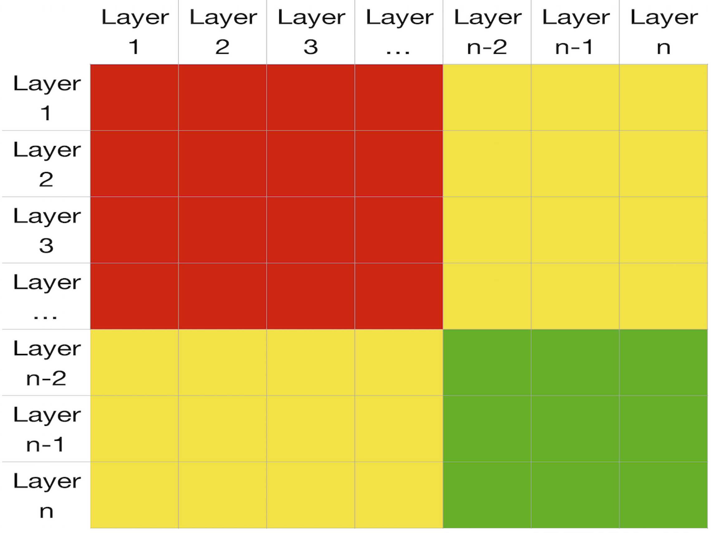
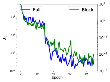
Figure 6: Illustration of block Hessian (left). Instead computing the top eigenvalue of whole Hessian, we just compute the eigenvalue of the green block. Top eigenvalues of Block of C1 (right) on Cifar-10. The block Hessian is computed by the last two layers of C1. The maximum batch size of C1 is 16000. The full Hessian is based on BL with batch size of 128.

Appendix D Additional empirical results

In this section, we present additional empirical results that were discussed in Section 4 (i.e., Table I-VIII, and Fig. 3).

TABLE III: Accuracy and the number of parameter updates of S1 on SVHN.

	BL		FB		GG		ABS		ABSA
BS	Acc.	# Iters	Acc.	# Iters	Acc.	# Iters	Acc.	# Iters	Acc.	# Iters
128	94.90	81986	N.A.	N.A.	N.A.	N.A.	N.A.	N.A.	N.A.	N.A.
512	94.76	20747	95.24	20747	95.49	51862	95.65	25353	95.72	24329
2048	95.17	5186	95.00	5186	95.59	45935	95.51	10562	95.82	16578
8192	93.73	1296	19.58	1296	95.70	44407	95.56	14400	95.61	7776
32768	91.03	324	10.00	324	95.60	42867	95.60	7996	95.90	12616
131072	84.75	81	10.00	81	95.58	42158	95.61	11927	95.92	11267

TABLE IV: Accuracy and the number of parameter updates of C1 on Cifar-10.

	BL		FB		GG		ABS		ABSA
BS	Acc.	# Iters	Acc.	# Iters	Acc.	# Iters	Acc.	# Iters	Acc.	# Iters
128	83.05	35156	N.A.	N.A.	N.A.	N.A.	N.A.	N.A.	N.A.	N.A.
640	81.01	7031	84.59	7031	83.99	16380	83.30	10578	84.52	9631
3200	74.54	1406	78.70	1406	84.27	14508	83.33	6375	84.42	5168
5120	70.64	878	74.65	878	83.47	14449	83.83	6575	85.01	6265
10240	68.75	439	30.99	439	83.68	14400	83.56	5709	84.29	7491
16000	67.88	281	10.00	281	84.00	14383	83.50	5739	84.24	5357

TABLE V: Accuracy and the number of parameter updates of C2 on Cifar-10.

	BL		FB		GG		ABS		ABSA
BS	Acc.	# Iters	Acc.	# Iters	Acc.	# Iters	Acc.	# Iters	Acc.	# Iters
128	87.64	35156	N.A.	N.A.	N.A.	N.A.	N.A.	N.A.	N.A.	N.A.
640	86.20	7031	87.9	7031	87.84	16380	87.86	10399	89.05	10245
3200	82.59	1406	73.2	1406	87.59	14508	88.02	5869	89.04	4525
5120	81.40	878	63.27	878	87.85	14449	87.92	7479	88.64	5863
10240	79.85	439	10.00	439	87.52	14400	87.84	5619	89.03	3929
16000	81.06	281	10.00	281	88.28	14383	87.58	9321	89.19	4610

TABLE VI: Accuracy and the number of parameter updates of C4 on Cifar-10.

	BL		FB		GG		ABS		ABSA
BS	Acc.	# Iters	Acc.	# Iters	Acc.	# Iters	Acc.	# Iters	Acc.	# Iters
128	93.25	78125	N.A.	N.A.	N.A.	N.A.	N.A.	N.A.	N.A.	N.A.
256	93.81	39062	89.51	39062	93.53	50700	93.47	43864	93.76	45912
512	93.61	19531	89.14	19531	93.87	37058	93.54	25132	93.57	28494
1024	91.51	9766	88.69	9766	93.21	31980	93.40	19030	93.26	22741
2048	87.90	4882	88.03	4882	93.54	30030	93.40	21387	93.50	23755
4096	80.77	2441	86.21	2441	93.32	29191	93.55	14245	93.82	20557

TABLE VII: Accuracy and the number of parameter updates of C5 on Cifar-100.

	BL		FB		GG		ABS		ABSA
BS	Acc.	# Iters	Acc.	# Iters	Acc.	# Iters	Acc.	# Iters	Acc.	# Iters
128	67.67	62500	N.A.	N.A.	N.A.	N.A.	N.A.	N.A.	N.A.	N.A
256	67.12	31250	67.89	31250	66.79	46800	67.71	33504	67.32	33760
512	66.47	15625	67.83	15625	67.74	39000	67.68	32240	67.87	24688
1024	64.7	7812	67.72	7812	67.17	35100	65.31	22712	68.03	13688
2048	62.91	3906	67.93	3906	67.76	33735	64.69	25180	68.43	12103

TABLE VIII: Accuracy and the number of parameter updates of I1 on TinyImageNet.

	BL		FB		GG		ABSA
BS	Acc.	# Iters	Acc.	# Iters	Acc.	# Iters	Acc.	# Iters
128	60.41	93750	N.A.	N.A.	N.A.	N.A.	N.A.	N.A.
256	58.24	46875	59.82	46875	60.31	70290	61.28	60684
512	57.48	23437	59.28	23437	59.94	58575	60.55	51078
1024	54.14	11718	59.62	11718	59.72	52717	60.72	19011
2048	50.89	5859	59.18	5859	59.82	50667	60.43	17313
4096	40.97	2929	58.26	2929	60.09	49935	61.14	22704
8192	25.01	1464	16.48	1464	60.00	49569	60.71	22334
16384	10.21	732	0.50	732	60.37	48995	60.71	20348

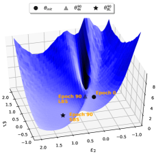
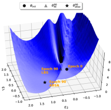
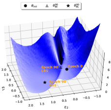
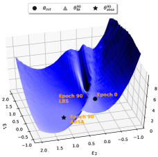
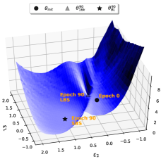
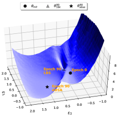
Figure 9: (left) 3D parametric plot for C1 model on Cifar-10. Points are labeled with the number of epochs (e.g. 90) and the technique that was used to arrive at that point (e.g. large batch size, LBS). The $\epsilon_{1}$ direction shows how the loss changes across the path between initial model at epoch 0, and the final model achieved with Large Batch Size (LBS) of $B=4K,~{}8K,~{}16K$. Similarly, $\epsilon_{2}$ direction computes loss when the model parameters are interpolated between epoch 0 and final model at epoch 90 with Small Batch Size(SBS). Notice the sharp curvature that Large Batch Size gets attracted to. On the right we show a similar plot except that we use ABSA algorithm with final batch of $16K$ rather than SGD with a small batch size for interpolating the $\epsilon_{2}$ direction. Notice the visual similarity between the point that ABSA converges to after 90 epochs (ABSA, 84.24% accuracy) and the point that small batch SGD (SBS, 83.05% accuracy) converges to after 90 epochs. Also note, that both avoid the sharp landscape that large batch gets attracted to sharper landscapes.

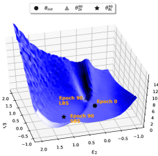
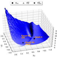
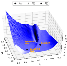
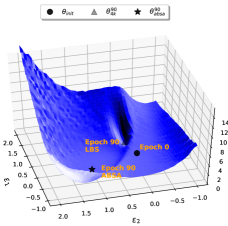
Figure 10: (left) 3D parametric plot for C2 model on Cifar-10. Points are labeled with the number of epochs (e.g. 90) and the technique that was used to arrive at that point (e.g. large batch size, LBS). The $\epsilon_{1}$ direction shows how the loss changes across the path between initial model at epoch 0, and the final model achieved with Large Batch Size (LBS) of $B=4K,~{}8K,~{}16K$. Similarly, $\epsilon_{2}$ direction computes loss when the model parameters are interpolated between epoch 0 and final model at epoch 90 with Small Batch Size(SBS). Notice the sharp curvature that Large Batch Size gets attracted to. On the right we show a similar plot except that we use ABSA algorithm with final batch of $16K$ rather than SGD with a small batch size for interpolating the $\epsilon_{2}$ direction. Notice the visual similarity between the point that ABSA converges to after 90 epochs (ABSA, 89.19% accuracy) and the point that small batch SGD (SBS, 87.64% accuracy) converges to after 90 epochs. Also note, that both avoid the sharp landscape that large batch gets attracted to sharper landscapes.

References

- [1] Alekh Agarwal and John C Duchi. Distributed delayed stochastic optimization. In NIPS, 2011.
- [2] Ioana Baldini, Paul Castro, Kerry Chang, Perry Cheng, Stephen Fink, Vatche Ishakian, Nick Mitchell, Vinod Muthusamy, Rodric Rabbah, Aleksander Slominski, et al. Serverless computing: Current trends and open problems. In Research Advances in Cloud Computing, pages 1–20. Springer, 2017.
- [3] Lukas Balles, Javier Romero, and Philipp Hennig. Coupling adaptive batch sizes with learning rates. arXiv:1612.05086, 2016.
- [4] Raghu Bollapragada, Richard Byrd, and Jorge Nocedal. Adaptive sampling strategies for stochastic optimization. SIAM Journal on Optimization, 28(4), 2018.
- [5] Raghu Bollapragada, Dheevatsa Mudigere, Jorge Nocedal, Hao-Jun Michael Shi, and Ping Tak Peter Tang. A progressive batching l-bfgs method for machine learning. arXiv:1802.05374, 2018.
- [6] Léon Bottou, Frank E Curtis, and Jorge Nocedal. Optimization methods for large-scale machine learning. SIAM Review, 60(2), 2018.
- [7] Richard H Byrd, Gillian M Chin, Jorge Nocedal, and Yuchen Wu. Sample size selection in optimization methods for machine learning. Mathematical programming, 134(1), 2012.
- [8] Nicholas Carlini and David Wagner. Towards evaluating the robustness of neural networks. In 2017 IEEE Symposium on Security and Privacy (SP). IEEE, 2017.
- [9] Yann N Dauphin, Razvan Pascanu, Caglar Gulcehre, Kyunghyun Cho, Surya Ganguli, and Yoshua Bengio. Identifying and attacking the saddle point problem in high-dimensional non-convex optimization. In NIPS, 2014.
- [10] Jia Deng, Wei Dong, Richard Socher, Li-Jia Li, Kai Li, and Li Fei-Fei. Imagenet: A large-scale hierarchical image database. In CVPR. Ieee, 2009.
- [11] Aditya Devarakonda, Maxim Naumov, and Michael Garland. Adabatch: Adaptive batch sizes for training deep neural networks. arXiv:1712.02029, 2017.
- [12] Michael P Friedlander and Mark Schmidt. Hybrid deterministic-stochastic methods for data fitting. SIAM Journal on Scientific Computing, 34(3), 2012.
- [13] Amir Gholami, Ariful Azad, Peter Jin, Kurt Keutzer, and Aydin Buluc. Integrated model, batch and domain parallelism in training neural networks. ACM SPAA’18, 2018.
- [14] Amir Gholami, Kiseok Kwon, Bichen Wu, Zizheng Tai, Xiangyu Yue, Peter Jin, Sicheng Zhao, and Kurt Keutzer. Squeezenext: Hardware-aware neural network design. CVPR Workshop, 2018.
- [15] Noah Golmant, Nikita Vemuri, Zhewei Yao, Vladimir Feinberg, Amir Gholami, Kai Rothauge, Michael W Mahoney, and Joseph Gonzalez. On the computational inefficiency of large batch sizes for stochastic gradient descent. arXiv:1811.12941, 2018.
- [16] Ian J Goodfellow, Jonathon Shlens, and Christian Szegedy. Explaining and harnessing adversarial examples. arXiv:1412.6572, 2014.
- [17] Priya Goyal, Piotr Dollár, Ross Girshick, Pieter Noordhuis, Lukasz Wesolowski, Aapo Kyrola, Andrew Tulloch, Yangqing Jia, and Kaiming He. Accurate, large minibatch sgd: training imagenet in 1 hour. arXiv:1706.02677, 2017.
- [18] Vipul Gupta, Swanand Kadhe, Thomas Courtade, Michael W Mahoney, and Kannan Ramchandran. Oversketched newton: Fast convex optimization for serverless systems. arXiv preprint arXiv:1903.08857, 2019.
- [19] Kaiming He, Xiangyu Zhang, Shaoqing Ren, and Jian Sun. Deep residual learning for image recognition. In CVPR, 2016.
- [20] HessianFlow. https://github.com/amirgholami/hessianflow, November 2018.
- [21] Andrew Ilyas, Shibani Santurkar, Dimitris Tsipras, Logan Engstrom, Brandon Tran, and Aleksander Madry. Adversarial examples are not bugs, they are features. arXiv:1905.02175, 2019.
- [22] Xianyan Jia, Shutao Song, Wei He, Yangzihao Wang, Haidong Rong, Feihu Zhou, Liqiang Xie, Zhenyu Guo, Yuanzhou Yang, Liwei Yu, et al. Highly scalable deep learning training system with mixed-precision: Training imagenet in four minutes. arXiv:1807.11205, 2018.
- [23] Nitish Shirish Keskar, Dheevatsa Mudigere, Jorge Nocedal, Mikhail Smelyanskiy, and Ping Tak Peter Tang. On large-batch training for deep learning: Generalization gap and sharp minima. arXiv:1609.04836, 2016.
- [24] Alex Krizhevsky and Geoffrey Hinton. Learning multiple layers of features from tiny images. Technical report, Citeseer, 2009.
- [25] Alex Krizhevsky, Ilya Sutskever, and Geoffrey E Hinton. Imagenet classification with deep convolutional neural networks. In NIPS, 2012.
- [26] Linjian Ma, Gabe Montague, Jiayu Ye, Zhewei Yao, Amir Gholami, Kurt Keutzer, and Michael W Mahoney. Inefficiency of k-fac for large batch size training. arXiv:1903.06237, 2019.
- [27] Saeed Maleki, Madanlal Musuvathi, and Todd Mytkowicz. Parallel stochastic gradient descent with sound combiners. arXiv:1705.08030, 2017.
- [28] James Martens. Deep learning via hessian-free optimization. In ICML, volume 27, 2010.
- [29] C. H. Martin and M. W. Mahoney. Implicit self-regularization in deep neural networks: Evidence from random matrix theory and implications for learning. Technical Report Preprint: arXiv:1810.01075, 2018.
- [30] C. H. Martin and M. W. Mahoney. Traditional and heavy-tailed self regularization in neural network models. In Proceedings of the 36th International Conference on Machine Learning, pages 4284–4293, 2019.
- [31] Sam McCandlish, Jared Kaplan, Dario Amodei, and OpenAI Dota Team. An empirical model of large-batch training. arXiv:1812.06162, 2018.
- [32] Hiroaki Mikami, Hisahiro Suganuma, Yoshiki Tanaka, Yuichi Kageyama, et al. Imagenet/resnet-50 training in 224 seconds. arXiv:1811.05233, 2018.
- [33] Seyed-Mohsen Moosavi-Dezfooli, Alhussein Fawzi, and Pascal Frossard. Deepfool: a simple and accurate method to fool deep neural networks. In CVPR, 2016.
- [34] Philipp Moritz, Robert Nishihara, Stephanie Wang, Alexey Tumanov, Richard Liaw, Eric Liang, Melih Elibol, Zongheng Yang, William Paul, Michael I Jordan, et al. Ray: A distributed framework for emerging ai applications. In 13th Symposium on Operating Systems Design and Implementation, 2018.
- [35] Yuval Netzer, Tao Wang, Adam Coates, Alessandro Bissacco, Bo Wu, and Andrew Y Ng. Reading digits in natural images with unsupervised feature learning. In NIPS, 2011.
- [36] Kazuki Osawa, Yohei Tsuji, Yuichiro Ueno, Akira Naruse, Rio Yokota, and Satoshi Matsuoka. Second-order optimization method for large mini-batch: Training resnet-50 on imagenet in 35 epochs. arXiv:1811.12019, 2018.
- [37] Tom Schaul, Sixin Zhang, and Yann LeCun. No more pesky learning rates. In ICML, 2013.
- [38] Uri Shaham, Yutaro Yamada, and Sahand Negahban. Understanding adversarial training: Increasing local stability of neural nets through robust optimization. arXiv:1511.05432, 2015.
- [39] Christopher J Shallue, Jaehoon Lee, Joe Antognini, Jascha Sohl-Dickstein, Roy Frostig, and George E Dahl. Measuring the effects of data parallelism on neural network training. arXiv:1811.03600, 2018.
- [40] Ashish Shrivastava, Tomas Pfister, Oncel Tuzel, Joshua Susskind, Wenda Wang, and Russell Webb. Learning from simulated and unsupervised images through adversarial training. In CVPR, 2017.
- [41] Samuel L Smith, Pieter-Jan Kindermans, and Quoc V Le. Don’t decay the learning rate, increase the batch size. arXiv:1711.00489, 2017.
- [42] Samuel L Smith and Quoc V Le. A Bayesian perspective on generalization and Stochastic Gradient Descent. arXiv:1710.06451, 2018.
- [43] Rajeev Thakur, Rolf Rabenseifner, and William Gropp. Optimization of collective communication operations in mpich. INT J HIGH PERFORM C, 2005.
- [44] Peng Xu, Farbod Roosta-Khorasan, and Michael W Mahoney. Second-order optimization for non-convex machine learning: An empirical study. arXiv:1708.07827, 2017.
- [45] Zhewei Yao, Amir Gholami, Kurt Keutzer, and Michael Mahoney. Pyhessian: Neural networks through the lens of the hessian. arXiv preprint arXiv:1912.07145, 2019.
- [46] Zhewei Yao, Amir Gholami, Qi Lei, Kurt Keutzer, and Michael W Mahoney. Hessian-based analysis of large batch training and robustness to adversaries. NIPS, 2018.
- [47] Zhewei et al. Yao. Trust region based adversarial attack on neural networks. In Proceedings of the IEEE Conference on Computer Vision and Pattern Recognition, pages 11350–11359, 2019.
- [48] Chris Ying, Sameer Kumar, Dehao Chen, Tao Wang, and Youlong Cheng. Image classification at supercomputer scale. arXiv:1811.06992, 2018.
- [49] Yang You, Igor Gitman, and Boris Ginsburg. Scaling sgd batch size to 32k for imagenet training. arXiv:1708.03888, 2017.
- [50] Sergey Zagoruyko and Nikos Komodakis. Wide residual networks. arXiv:1605.07146, 2016.
- [51] Sixin Zhang, Anna E Choromanska, and Yann LeCun. Deep learning with elastic averaging sgd. In NIPS, 2015.
- [52] Shuxin Zheng, Qi Meng, Taifeng Wang, Wei Chen, Nenghai Yu, Zhi-Ming Ma, and Tie-Yan Liu. Asynchronous stochastic gradient descent with delay compensation. arXiv:1609.08326, 2016.
- [53] Zhanxing Zhu, Jingfeng Wu, Bing Yu, Lei Wu, and Jinwen Ma. The anisotropic noise in stochastic gradient descent: Its behavior of escaping from minima and regularization effects. arXiv:1803.00195, 2018.