Causal inference under over-simplified longitudinal causal models

*Corresponding author: Lola Étiévant, Institut Camille Jordan, Villeurbanne 69622, France, E-mail: lola.etievant@gmail.com. https://orcid.org/0000-0001-7562-3550

Vivian Viallon, Nutritional Methodology and Biostatistics, International Agency for Research on Cancer, Lyon 69372, France, E-mail: viallonv@iarc.fr

The final published article and its Supplementary Materials are available at the International Journal of Biostatistics website.

Abstract

Many causal models of interest in epidemiology involve longitudinal exposures, confounders and mediators. However, repeated measurements are not always available or used in practice, leading analysts to overlook the time-varying nature of exposures and work under over-simplified causal models. Our objective is to assess whether - and how - causal effects identified under such misspecified causal models relates to true causal effects of interest. We derive sufficient conditions ensuring that the quantities estimated in practice under over-simplified causal models can be expressed as weighted averages of longitudinal causal effects of interest. Unsurprisingly, these sufficient conditions are very restrictive, and our results state that the quantities estimated in practice should be interpreted with caution in general, as they usually do not relate to any longitudinal causal effect of interest. Our simulations further illustrate that the bias between the quantities estimated in practice and the weighted averages of longitudinal causal effects of interest can be substantial. Overall, our results confirm the need for repeated measurements to conduct proper analyses and/or the development of sensitivity analyses when they are not available.

Keywords: Causal inference, longitudinal model, identifiability, structural causal model.

1 Introduction

Etiologic epidemiology is concerned with the study of potential causes of chronic diseases based on observational data. Over the years, it has been successful in the identification of links between several lifestyle exposures and the risk of cancer for example. Remarkable examples are tobacco smoke, alcohol and obesity that are now established risk factors for the development of a number of site-specific cancers (Agudo et al.,, 2012, Bagnardi et al.,, 2015, Lauby-Secretan et al.,, 2016). Moreover, an accumulating body of biomarker measurements and -omics data provide important opportunities for investigating biological mechanisms potentially involved in cancer development. For example, cancer epidemiology is increasingly concerned by the study of the carcinogenic role of inflammation, insulin resistance and sex steroids hormones (Bradbury et al.,, 2019, Chan et al.,, 2011, Dossus et al.,, 2013).

As they are based on observational data, the causal validity of these analyses relies on strong assumptions, which have been formally described in the causal inference literature (Hernan and Robins,, 2020, Pearl, 2009a, , Pearl, 2009b, , Rosenbaum and Rubin,, 1983, Robins,, 1986). The very first assumption underlying most causal analyses is that the causal model is correctly specified. Most often, e.g., when studying lifestyle exposures such as tobacco smoke, alcohol and obesity, but also biomarkers, the true causal model involves time-varying risk factors. Valid causal inference under such longitudinal causal models usually requires repeated measurements for the time-varying variables (Daniel et al.,, 2012, VanderWeele,, 2015, VanderWeele and Tchetgen Tchetgen,, 2017). However, repeated measurements are still rarely available in large prospective epidemiological studies; exceptions include electronic health records, but their analyses raise other challenges (see Section 5). Issues arising when ignoring the time-dependant nature of the exposures have been described in the literature (Aalen et al.,, 2016, Maxwell and Cole,, 2007, Maxwell et al.,, 2011). Moreover, general results on the identifiability of causal effects in the presence of unobserved variables can be used to study the identifiability of causal effects of interest when ignoring the time-varying nature of exposures (Shpitser and Pearl,, 2006, Tian and Pearl,, 2002, Huang and Valtorta,, 2006, Tian and Pearl,, 2003).

However, little is known about the possible relationship between estimates derived under oversimplified longitudinal causal models and causal quantities of interest under the true longitudinal causal model. Filling this gap is the main objective of the present work. Specifically, we derive sufficient conditions that guarantee that the quantity estimated in practice when working under over-simplified causal models is related to longitudinal causal effects of interest. Unsurprisingly, these sufficient conditions are very restrictive, and are met under very simple causal models only. Through numerical examples, we show that the magnitude of the bias between the quantities estimated in practice and longitudinal causal effects of interest can be substantial. Overall, our results raise the need for repeated measurements to conduct proper analyses and/or the development of sensitivity analyses when they are not available.

The rest of the article is organized as follows. The notation and framework considered in this work is introduced in Section 2. In section 3, we present our main result and discuss its practical implications. Section 4 is devoted to numerical illustrations. Concluding remarks are provided in Section 5. Technical derivations are presented in the Appendix.

2 Notation

2.1 The true longitudinal causal model

We consider standard longitudinal causal models (Daniel et al.,, 2012, VanderWeele,, 2015), where time-varying exposures, including the exposure of interest, but also possibly mediators and confounders, are observable at discrete times over the time-window $\llbracket 1;T\rrbracket:=\{1,\ldots,T\}$, for some time $T>1$. For any $t\in\llbracket 1;T\rrbracket$, we denote by $X_{t}$ the exposure of interest at time $t$, by $\bar{X}_{t}=(X_{1},X_{2},\dots,X_{t})$ the exposure profile until time $t$, while $\bar{x}_{t}$ stands for a specific (fixed) profile for the exposure of interest (VanderWeele,, 2015). In addition, $\underline{X}_{t_{1}}^{t_{2}}=(X_{t_{1}},X_{t_{1}+1},\dots,X_{t_{2}})$ denotes the exposure profile from time $t_{1}$ to time $t_{2}$, $1\leq t_{1}\leq t_{2}\leq T$. We use similar notation for auxiliary factors $(Z_{t})_{t}$, which may include “pure mediator” processes $(M_{t})_{t}$ and confounder processes $(W_{t})_{t}$ possibly affected by the exposure of interest (as in Figure 1). By “pure mediator” process, we mean that $M_{t}$ does not affect $X_{t_{1}}$, for any $t,t_{1}\in\llbracket 1;T\rrbracket$, so that variables $(M_{t})_{t}$ only act as mediators (and not as confounders) in the relationship between the exposure of interest and the outcome. Similarly, a “pure confounder” refers to a variable, or process, that possibly affects, but is not affected by, the exposure. We denote by $Y$ the outcome of interest measured at time $T$. For example $(X_{t})_{t}$ could represent body mass index (BMI) at different ages, $Y$ could represent cancer development by a given age, while the auxiliary multivariate variable $(Z_{t})_{t}$ could represent alcohol intake, physical activity and dietary exposures at different ages. For illustration, we will mostly consider the example of the longitudinal causal model $(L.1)$ provided in Figure 1, as well as special cases of this model. Unless otherwise stated, we further assume that all variables are binary to simplify our notation.

($L.1$)

Figure 1: (L.1) Example of longitudinal causal model with a time-varying confounder $(W_{t})_{t\geq 1}$ possibly affected by the time-varying exposure of interest $(X_{t})_{t\geq 1}$.

For any pair of variables $(V,U)$ and any potential value $u$ of $U$, we denote by $V^{U=u}$ the counterfactual variable corresponding to variable $V$ that would have been observed in the counterfactual world following the hypothetical intervention $do(U=u)$. We work under the setting of Structural Causal Models (Pearl, 2009a, ), which especially entails that consistency conditions hold: for instance, $U=u$ implies $V=V^{U=u}$. In addition, some positivity conditions (Rosenbaum and Rubin,, 1983), specified in the conditions of Theorem 1 in Section 3, will be assumed to hold. For any possibly counterfactual random variables $V$ and $U$, and any causal model $(Mod)$, we use the notation $(V\mathbin{\mathchoice{\hbox to0.0pt{\hbox{\set@color$\displaystyle\perp$}\hss}\kern 3.46875pt{}\kern 3.46875pt\hbox{\set@color$\displaystyle\perp$}}{\hbox to0.0pt{\hbox{\set@color$\textstyle\perp$}\hss}\kern 3.46875pt{}\kern 3.46875pt\hbox{\set@color$\textstyle\perp$}}{\hbox to0.0pt{\hbox{\set@color$\scriptstyle\perp$}\hss}\kern 2.36812pt{}\kern 2.36812pt\hbox{\set@color$\scriptstyle\perp$}}{\hbox to0.0pt{\hbox{\set@color$\scriptscriptstyle\perp$}\hss}\kern 1.63437pt{}\kern 1.63437pt\hbox{\set@color$\scriptscriptstyle\perp$}}}U)_{Mod}$ to denote independence between variables $V$ and $U$ under the causal model ($Mod$). We further let $\mathbb{E}_{Mod}\left(V^{U=u}\right)$ be the expectation of variable $V^{U=u}$ under causal model (Mod). We will mostly consider such expectations for (Mod) set to either the true longitudinal causal model $(L)$ or the over-simplified model $(S)$ used for the analysis (see Section 2.2). Because expectations and probabilities involving observable variables only will always be computed under the true longitudinal causal model ($L$), we simply write $\mathbb{E}(V)$ and $\mathbb{P}(V=v)$ for any observable variable $V$ and any potential value $v$ of $V$, instead of $\mathbb{E}_{L}(V)$ and $\mathbb{P}_{L}(V=v)$, respectively.

In this framework, the causal effect of interest is that of the time-varying exposure $(X_{t})_{t}$ on the outcome $Y$, and a key quantity in our work is therefore

$$ATE_{L}\left(\underline{x}_{t_{0}}^{t_{3}};\underline{x}_{t_{1}}^{t_{2}*}\right)=\mathbb{E}_{L}\left(Y^{\underline{X}_{t_{0}}^{t_{3}}=\underline{x}_{t_{0}}^{t_{3}}}-Y^{\underline{X}_{t_{0}}^{t_{3}}=\underline{x}_{t_{0}}^{t_{3}*}}\right),$$ (1)

for given profiles $\underline{x}_{t_{0}}^{t_{3}}$ and $\underline{x}_{t_{0}}^{t_{3}*}$ for the exposure of interest, and given times $1\leq t_{0}\leq t_{3}\leq T$. This quantity is one measure of the total causal effect of the exposure from time $t_{0}$ to time $t_{3}$ on the outcome $Y$, under the longitudinal causal model $(L)$ (Daniel et al.,, 2012, VanderWeele,, 2015). In particular, total causal effects of the exposure over the full time interval may be considered ($t_{0}=1$, $t_{3}=T$), but other total causal effects, including that of the exposure at a single time point ($t_{0}=t_{3}$) can be considered as well under this longitudinal setting. Because the causal effect in Equation (1) generally depends on the particular profiles $\underline{x}_{t_{0}}^{t_{3}}$ and $\underline{x}_{t_{0}}^{t_{3}*}$, averaged total effects can be defined as

$$\sum_{\underline{x}_{t_{0}}^{t_{3}}}\sum_{\underline{x}_{t_{0}}^{t_{3}*}}ATE_{L}\left(\underline{x}_{t_{0}}^{t_{3}};\underline{x}_{t_{0}}^{t_{3}*}\right)\omega\left(\underline{x}_{t_{0}}^{t_{3}},\underline{x}_{t_{0}}^{t_{3}*}\right),$$

for appropriate weights $\omega(\underline{x}_{t_{0}}^{t_{3}},\underline{x}_{t_{0}}^{t_{3}*})$, and with the two sums over $\{0,1\}\times\dots\times\{0,1\}=\{0,1\}^{t_{3}-t_{0}+1}$. For future use, we also introduce stratum-specific causal effects (Hernan and Robins,, 2020), with strata defined according to the levels of a possibly multivariate variable $U$

$$ATE_{L_{\mid U=u}}\left(\underline{x}_{t_{0}}^{t_{3}};\underline{x}_{t_{0}}^{t_{3}*}\right):=\mathbb{E}_{L}\left(Y^{\underline{X}_{t_{0}}^{t_{3}}=\underline{x}_{t_{0}}^{t_{3}}}-Y^{\underline{X}_{t_{0}}^{t_{3}}=\underline{x}_{t_{0}}^{t_{3}*}}\mid U=u\right).$$ (2)

Weighted averages of the form $\sum_{u}\sum_{\underline{x}_{t_{0}}^{t_{3}}}\sum_{\underline{x}_{t_{0}}^{t_{3}*}}ATE_{L_{\mid U=u}}\left(\underline{x}_{t_{0}}^{t_{3}};\underline{x}_{t_{0}}^{t_{3}*}\right)\omega\left(\underline{x}_{t_{0}}^{t_{3}},\underline{x}_{t_{0}}^{t_{3}*},u\right)$ will also be considered for appropriate weights $\omega\left(\underline{x}_{t_{0}}^{t_{3}},\underline{x}_{t_{0}}^{t_{3}*},u\right)$.

2.2 The over-simplified causal model considered in practice

Often, analysts do not have access to, or simply ignore, the full exposures profiles ($\bar{X}_{T},\bar{Z}_{T}$), and focus on “summaries” $(\mathcall{X},\mathcall{Z})$ of ($\bar{X}_{T},\bar{Z}_{T}$) instead, with $\mathcall{X}=f_{X}(\bar{X}_{T})$ and $\mathcall{Z}=f_{Z}(\bar{Z}_{T})$, for two given deterministic functions $f_{X}$ and $f_{Z}$. The most common case in practice is when $\mathcall{X}=X_{t}$ and $\mathcall{Z}=Z_{t}$, for some time $t\in\llbracket 1;T\rrbracket$, e.g., the time of inclusion in the study. But $\mathcall{X}$ and $\mathcall{Z}$ can represent other summaries of ($\bar{X}_{T},\bar{Z}_{T}$), such as $(i)$ cumulative exposure over some time-interval: $\mathcall{X}=\sum_{t=t_{1}}^{t_{2}}X_{t}$ for some $1\leq t_{1}\leq t_{2}\leq T$; or $(ii)$ duration of exposure over a certain threshold $\mathcall{X}=\mathbb{1}\{\sum_{t=t_{1}}^{t_{2}}X_{t}\geq\tau\}$ for some threshold $\tau\in\mathbb{R}$ (Arnold et al.,, 2016, Kunzmann et al.,, 2018, De Rubeis et al.,, 2019, Yang et al.,, 2019, Zheng et al.,, 2018, Fan et al.,, 2008, Platt et al.,, 2010, Arnold et al.,, 2019). Moreover, $f_{X}$ and $f_{Z}$ do not have to share the same form; for example, we can have $\mathcall{Z}=Z_{t_{1}}$ and $\mathcall{X}=\sum_{t=t_{1}}^{t_{2}}X_{t}$. Lastly, some components of $\mathcall{Z}$ may be unobserved in practice.

When focusing on $\mathcall{X}$ and $\mathcall{Z}$, analysts generally ignore $\bar{X}_{T}$ and $\bar{Z}_{T}$ and work under an over-simplified causal model (S), which only involves $\mathcall{X}$, $\mathcall{Z}$ and $Y$. For example, if the true causal model is model $(L.1)$ of Figure 1 but only summaries $\mathcall{X}$ and $\mathcall{W}$ of $\bar{X}_{T}$ and $\bar{W}_{T}$ are available or considered, analysts may be tempted to work under the simplified causal models $(S.1)$ or $(S.2)$ of Figure 2, depending on whether $(W_{t})_{t\leq 1}$ is mainly regarded as a confounder or as a mediator. Consequently, they also generally consider $ATE_{S}\left(\mathcall{x};\mathcall{x}^{*}\right)=\mathbb{E}_{S}\big{(}Y^{\mathcall{X}=\mathcall{x}}-Y^{\mathcall{X}=\mathcall{x}^{*}}\big{)}$, for any $\mathcall{x}\neq\mathcall{x}^{*}$, as the causal effect of interest. If there exists some observed $\mathcall{W}\subset\mathcall{Z}$ taking its values in $\Omega_{\mathcall{W}}$, such that $(Y^{\mathcall{X}=\mathcall{x}}\mathbin{\mathchoice{\hbox to0.0pt{\hbox{\set@color$\displaystyle\perp$}\hss}\kern 3.46875pt{}\kern 3.46875pt\hbox{\set@color$\displaystyle\perp$}}{\hbox to0.0pt{\hbox{\set@color$\textstyle\perp$}\hss}\kern 3.46875pt{}\kern 3.46875pt\hbox{\set@color$\textstyle\perp$}}{\hbox to0.0pt{\hbox{\set@color$\scriptstyle\perp$}\hss}\kern 2.36812pt{}\kern 2.36812pt\hbox{\set@color$\scriptstyle\perp$}}{\hbox to0.0pt{\hbox{\set@color$\scriptscriptstyle\perp$}\hss}\kern 1.63437pt{}\kern 1.63437pt\hbox{\set@color$\scriptscriptstyle\perp$}}}\mathcall{X}\mid\mathcall{W})_{S}$, as under model ($S.1$) of Figure 2, and if some positivity condition holds (Rosenbaum and Rubin,, 1983), analysts would identify, and then estimate, $ATE_{S}\left(\mathcall{x};\mathcall{x}^{*}\right)$ as

$$\sum_{\mathcall{w}\in\Omega_{\mathcall{W}}}\left[\mathbb{E}\left(Y\mid\mathcall{W}=\mathcall{w},\mathcall{X}=\mathcall{x}\right)-\mathbb{E}\left(Y\mid\mathcall{W}=\mathcall{w},\mathcall{X}=\mathcall{x}^{*}\right)\right]\times\mathbb{P}(\mathcall{W}=\mathcall{w}).$$

Conversely, if $(Y^{\mathcall{X}=\mathcall{x}}\mathbin{\mathchoice{\hbox to0.0pt{\hbox{\set@color$\displaystyle\perp$}\hss}\kern 3.46875pt{}\kern 3.46875pt\hbox{\set@color$\displaystyle\perp$}}{\hbox to0.0pt{\hbox{\set@color$\textstyle\perp$}\hss}\kern 3.46875pt{}\kern 3.46875pt\hbox{\set@color$\textstyle\perp$}}{\hbox to0.0pt{\hbox{\set@color$\scriptstyle\perp$}\hss}\kern 2.36812pt{}\kern 2.36812pt\hbox{\set@color$\scriptstyle\perp$}}{\hbox to0.0pt{\hbox{\set@color$\scriptscriptstyle\perp$}\hss}\kern 1.63437pt{}\kern 1.63437pt\hbox{\set@color$\scriptscriptstyle\perp$}}}\mathcall{X})_{S}$, as under models ($S.2$) and ($S.3$) of Figure 2, analysts would simply identify $ATE_{S}\left(\mathcall{x};\mathcall{x}^{*}\right)$ as $\mathbb{E}\left(Y\mid\mathcall{X}=\mathcall{x}\right)-\mathbb{E}\left(Y\mid\mathcall{X}=\mathcall{x}^{*}\right)$. We will thereafter denote by $\widetilde{ATE}_{S}(\mathcall{x};\mathcall{x}^{*})$ the observable quantity estimated in practice when working under the simplified causal model $(S)$.

($S.1$)

($S.2$)

($S.3$)

Figure 2: Examples of over-simplified causal models.

3 Main result

3.1 Statement

Because, the true causal model ($L$) involves the time-varying exposure of interest and time-varying auxiliary variables (see for example model ($L.1$) in Figure 1), a natural question is whether - and how - this quantity $\widetilde{ATE}_{S}\left(\mathcall{x};\mathcall{x}^{*}\right)$ relates to causal effects of interest under the true longitudinal causal model $(L)$. Theorem 1 below presents a sufficient condition under which the quantity $\widetilde{ATE}_{S}\left(\mathcall{x};\mathcall{x}^{*}\right)$ estimated in practice can be written as a weighted average of (possibly stratum-specific) longitudinal total effects.

Theorem 1.

Assume that the observed $\mathcal{X}$ is a deterministic function of $\underline{X}_{t_{1}}^{t_{2}}$ for some $1\leq t_{1}\leq t_{2}\leq T$. For any possible values $\mathcall{x}$ and $\mathcall{x}^{*}$ of $\mathcal{X}$, if condition $(T.Cond)$ below holds

• (T.Cond)  There exists some $t_{0}\in\llbracket 1,t_{1}\rrbracket$, some $t_{3}\in\llbracket t_{2},T\rrbracket$ and some observed $\mathcall{W}\subset\mathcall{Z}$ taking its values in $\Omega_{\mathcall{W}}$, such that $(Y^{\mathcall{X}=\mathcall{x}}\mathbin{\mathchoice{\hbox to0.0pt{\hbox{\set@color$\displaystyle\perp$}\hss}\kern 3.46875pt{}\kern 3.46875pt\hbox{\set@color$\displaystyle\perp$}}{\hbox to0.0pt{\hbox{\set@color$\textstyle\perp$}\hss}\kern 3.46875pt{}\kern 3.46875pt\hbox{\set@color$\textstyle\perp$}}{\hbox to0.0pt{\hbox{\set@color$\scriptstyle\perp$}\hss}\kern 2.36812pt{}\kern 2.36812pt\hbox{\set@color$\scriptstyle\perp$}}{\hbox to0.0pt{\hbox{\set@color$\scriptscriptstyle\perp$}\hss}\kern 1.63437pt{}\kern 1.63437pt\hbox{\set@color$\scriptscriptstyle\perp$}}}\mathcall{X}\mid\mathcall{W})_{S}$, $0<\mathbb{P}(\mathcall{X}=\mathcall{x}\mid\mathcall{W}=\mathcall{w})<1$, $0<\mathbb{P}(\mathcall{X}=\mathcall{x}^{*}\mid\mathcall{W}=\mathcall{w})<1$, for all $\mathcall{w}$ such that $0<\mathbb{P}(\mathcall{W}=\mathcall{w})$, and $(Y^{\underline{X}_{t_{0}}^{t_{3}}=\underline{x}_{t_{0}}^{t_{3}}}\mathbin{\mathchoice{\hbox to0.0pt{\hbox{\set@color$\displaystyle\perp$}\hss}\kern 3.46875pt{}\kern 3.46875pt\hbox{\set@color$\displaystyle\perp$}}{\hbox to0.0pt{\hbox{\set@color$\textstyle\perp$}\hss}\kern 3.46875pt{}\kern 3.46875pt\hbox{\set@color$\textstyle\perp$}}{\hbox to0.0pt{\hbox{\set@color$\scriptstyle\perp$}\hss}\kern 2.36812pt{}\kern 2.36812pt\hbox{\set@color$\scriptstyle\perp$}}{\hbox to0.0pt{\hbox{\set@color$\scriptscriptstyle\perp$}\hss}\kern 1.63437pt{}\kern 1.63437pt\hbox{\set@color$\scriptscriptstyle\perp$}}}\underline{X}_{t_{0}}^{t_{3}}\mid\mathcall{W})_{L}$,

then the quantity estimated in practice

$$\widetilde{ATE}_{S}\left(\mathcall{x};\mathcall{x}^{*}\right) = \sum_{\mathcall{w}\in\Omega_{\mathcall{W}}}\left[\mathbb{E}\left(Y\mid\mathcall{W}=\mathcall{w},\mathcall{X}=\mathcall{x}\right)-\mathbb{E}\left(Y\mid\mathcall{W}=\mathcall{w},\mathcall{X}=\mathcall{x}^{*}\right)\right]$$

$$\hskip 34.14322pt\times\mathbb{P}(\mathcall{W}=\mathcall{w}),$$

equals

$$\sum_{\mathcall{w}\in\Omega_{\mathcall{W}}}\sum_{\begin{subarray}{c}\underline{x}_{t_{0}}^{t_{3}}\in\{0,1\}^{t_{3}-t_{0}+1}\\ \underline{x}_{t_{0}}^{t_{3}*}\in\{0,1\}^{t_{3}-t_{0}+1}\end{subarray}}\{ATE_{L_{\mid\mathcall{W}=\mathcall{w}}}\left(\underline{x}_{t_{0}}^{t_{3}};\underline{x}_{t_{0}}^{t_{3}*}\right)\times\mathbb{P}(\underline{X}_{t_{0}}^{t_{3}}=\underline{x}_{t_{0}}^{t_{3}}\mid\mathcall{X}=\mathcall{x},\mathcall{W}=\mathcall{w})$$

$$\hskip 194.90155pt\times\mathbb{P}(\underline{X}_{t_{0}}^{t_{3}}=\underline{x}_{t_{0}}^{t_{3}*}\mid\mathcall{X}=\mathcall{x}^{*},\mathcall{W}=\mathcall{w})$$

$$\hskip 194.90155pt\times\mathbb{P}(\mathcall{W}=\mathcall{w})\}.$$ (3)

In particular, if condition $(T.Uncond)$ below holds

• $(T.Uncond)$ There exists some $t_{0}\in\llbracket 1,t_{1}\rrbracket$ and some $t_{3}\in\llbracket t_{2},T\rrbracket$ such that  $(Y^{\mathcall{X}=\mathcall{x}}\mathbin{\mathchoice{\hbox to0.0pt{\hbox{\set@color$\displaystyle\perp$}\hss}\kern 3.46875pt{}\kern 3.46875pt\hbox{\set@color$\displaystyle\perp$}}{\hbox to0.0pt{\hbox{\set@color$\textstyle\perp$}\hss}\kern 3.46875pt{}\kern 3.46875pt\hbox{\set@color$\textstyle\perp$}}{\hbox to0.0pt{\hbox{\set@color$\scriptstyle\perp$}\hss}\kern 2.36812pt{}\kern 2.36812pt\hbox{\set@color$\scriptstyle\perp$}}{\hbox to0.0pt{\hbox{\set@color$\scriptscriptstyle\perp$}\hss}\kern 1.63437pt{}\kern 1.63437pt\hbox{\set@color$\scriptscriptstyle\perp$}}}\mathcall{X})_{S}$, $0<\mathbb{P}(\mathcall{X}=\mathcall{x})<1$, $0<\mathbb{P}(\mathcall{X}=\mathcall{x}^{*})<1$, and $(Y^{\underline{X}_{t_{0}}^{t_{3}}=\underline{x}_{t_{0}}^{t_{3}}}\mathbin{\mathchoice{\hbox to0.0pt{\hbox{\set@color$\displaystyle\perp$}\hss}\kern 3.46875pt{}\kern 3.46875pt\hbox{\set@color$\displaystyle\perp$}}{\hbox to0.0pt{\hbox{\set@color$\textstyle\perp$}\hss}\kern 3.46875pt{}\kern 3.46875pt\hbox{\set@color$\textstyle\perp$}}{\hbox to0.0pt{\hbox{\set@color$\scriptstyle\perp$}\hss}\kern 2.36812pt{}\kern 2.36812pt\hbox{\set@color$\scriptstyle\perp$}}{\hbox to0.0pt{\hbox{\set@color$\scriptscriptstyle\perp$}\hss}\kern 1.63437pt{}\kern 1.63437pt\hbox{\set@color$\scriptscriptstyle\perp$}}}\underline{X}_{t_{0}}^{t_{3}})_{L}$

then

$$\widetilde{ATE}_{S}(\mathcall{x};\mathcall{x}^{*}) = \mathbb{E}\left(Y\mid\mathcall{X}=\mathcall{x}\right)-\mathbb{E}\left(Y\mid\mathcall{X}=\mathcall{x}^{*}\right),$$ (4)

$$= \sum_{\begin{subarray}{c}\underline{x}_{t_{0}}^{t_{3}}\in\{0,1\}^{t_{3}-t_{0}+1}\\ \underline{x}_{t_{0}}^{t_{3}*}\in\{0,1\}^{t_{3}-t_{0}+1}\end{subarray}}\{ATE_{L}\left(\underline{x}_{t_{0}}^{t_{3}};\underline{x}^{t_{3}*}_{t_{0}}\right)\times\mathbb{P}(\underline{X}_{t_{0}}^{t_{3}}=\underline{x}_{t_{0}}^{t_{3}}\mid\mathcall{X}=\mathcall{x})$$

$$\hskip 147.95424pt\times\mathbb{P}(\underline{X}_{t_{0}}^{t_{3}}=\underline{x}_{t_{0}}^{t_{3}*}\mid\mathcall{X}=\mathcall{x}^{*})\}.$$

The proof of Theorem 1 is given in Appendix A. Theorem 1 states that when $\mathcall X$ depends on the exposure profile from time $t_{1}$ to time $t_{2}$ and there exists a possibly empty set of observed variables that satisfies (i) the ignorability condition for the exposure profile on a possibly wider time-window and the outcome under the true longitudinal model, and (ii) the ignorability condition for $\mathcall{X}$ and the outcome under the over-simplified causal model, then the quantity estimated in practice expresses as a weighted average of possibly stratum-specific longitudinal total effects. Through the inspection of a few simple examples, we show in Section 3.2 that conditions $(T.Uncond)$ and $(T.Cond)$ are very restrictive, which confirms that the result of Theorem 1 is rarely valid in practice and that caution is usually required when interpreting the quantity estimated in practice. Indeed, even if conditions of Theorem 1 are sufficient conditions only, the quantity estimated in practice can generally not be expressed as the weighted average of any longitudinal effects of interest when they are not satisfied; see the Supplementary Material 1 and 2 for more details. Also, we show in Section 3.3 that even when the conditions of Theorem 1 are satisfied, the interpretation of the weighted averages, hence that of the quantity estimated in practice, is sometimes not straightforward.

3.2 About the conditions of Theorem 1

First, the presence of times $t_{0}\in\llbracket 1,t_{1}\rrbracket$ and $t_{3}\in\llbracket t_{2},T\rrbracket$ in conditions ($T.Cond$) and ($T.Uncond$) allows Theorem 1 to cover more general configurations, e.g., $(i)$ when $\mathcall{X}$ and $\mathcall{Z}$ are summaries of $\bar{X}_{T}$ and $\bar{Z}_{T}$ over different sub-intervals of $\llbracket 1,T\rrbracket$; or $(ii)$, when $\mathcall X=X_{t_{2}}$ and $\mathcall Z=Z_{t_{2}}$, for some time $t_{2}\in\llbracket 1;T\rrbracket$. Specifically, condition ($T.Uncond$) of Theorem is satisfied with $t_{0}=1$ and $t_{3}=t_{2}$ if the true causal model and simplified model are models $(L.0)$ and $(S.0)$ of Figure 3, respectively, and $\mathcall{X}=X_{t_{2}}$.

(L.0)

(S.0)

Figure 3: (L.0) Example of longitudinal model with a time-varying exposure of interest $(X_{t})_{t\geq 1}$, in the absence of confounding. (S.0) Over-simplified causal model associated with the longitudinal model (L.0), when data on the exposure is considered at time $t_{2}$ only.

Second, conditions ($T.Cond$) and ($T.Uncond$) of Theorem 1 are not testable, but the backdoor criterion can be applied to the DAGs corresponding to models $(S)$ and $(L)$, respectively, to check their validity (assuming these DAGs are well specified). For the true causal model $(L)$, the “augmented” DAG where summary variables $\mathcall{X}$ and $\mathcall{W}$ are explicitly represented should be considered. For example, under the longitudinal causal model $(L.1)$ of Figure 1, and assuming that the observed summary variables $\mathcall{X}$ and $\mathcall{W}$ are functions of the full exposure profiles $\bar{X}_{T}$ and $\bar{W}_{T}$ (that is, $t_{1}=1$ and $t_{2}=T$), possible augmented DAGs are presented in Figure 4, depending on whether these summary variables capture the whole effect of $\bar{X}_{T}$ and $\bar{W}_{T}$ on $Y$ or not. In either case, neither $\mathcall{W}$ nor the empty set satisfies the backdoor criterion relative to $\bar{X}_{T}$ and $Y$ in these augmented DAGs, so neither ($T.Cond$) nor ($T.Uncond$) is satisfied, and Theorem 1 does not apply.

(a)

(b)

Figure 4: Possible (augmented) DAGs corresponding to longitudinal causal model associated with model (L.1) given in Figure 1, depending on whether summaries $\mathcall W$ and $\mathcall{X}$ do not (a) or do (b) catpure the whole effect of $\bar{W}_{T}$ and $\bar{X}_{T}$ on $Y$.

Conversely, if the summary variables $\mathcall{X}$ and $\mathcall{W}$ capture the whole effect of $\bar{X}_{T}$ and $\bar{W}_{T}$, conditions of Theorem 1 are satisfied in either ($i$) the pure confounder setting of model ($L.2$) of Figure 5 (if, in addition, the over-simplified model is model ($S.1$) of Figure 2) or ($ii$) the pure mediator setting of model ($L.3$) of Figure 5 (if the over-simplified model is model ($S.2$), or ($S.3$), of Figure 2). When working under model ($S.1$) while the true causal model is ($L.2$), condition ($T.Cond$) holds and Theorem 1 states that $\widetilde{ATE}_{S}(\mathcall{x};\mathcall{x}^{*})$ is the weighted average of the longitudinal total effects given in Equation (3). When working under model ($S.2$) (or ($S.3$)) while the true causal model is ($L.3$), condition ($T.Uncond$) holds and Theorem 1 states that $\widetilde{ATE}_{S}(\mathcall{x};\mathcall{x}^{*})$ is the weighted average of the longitudinal total effects given in Equation (4). Interestingly, the conditions of Theorem 1 are not satisfied when the true causal model is model ($L.4$) of Figure 6, where both a pure time-varying confounder and a pure time-varying mediator that is affected by the confounder are present. Indeed, again, neither ($T.Cond$) nor ($T.Uncond$) is satisfied, and Theorem 1 does not apply. This is in sharp contrast with the setting of model ($L.2$), where only a time-varying pure confounder, and no time-varying pure mediator, is present, and in which case Theorem 1 applies. In other words, although generally overlooked when the focus is on total effects, the presence of a time-varying mediator affected by a pure confounder precludes the validity of Theorem 1.

(L.2)

(L.3)

Figure 5: (L.2) Example of a longitudinal causal model with a time-varying exposure of interest $(X_{t})_{t\geq 1}$ and a time-varying pure confounder $(W_{t})_{t\geq 1}$. (L.3) Example of a longitudinal causal model with a time-varying exposure of interest $(X_{t})_{t\geq 1}$ and a time-varying pure mediator $(M_{t})_{t\geq 1}$. In both cases, exposures of interest, confounders and mediators are assumed to affect the outcome through the observed summary variables only.

(L.4)

(S.4)

Figure 6: (L.4) Compact representation of a longitudinal model with a time-varying exposure of interest $(X_{t})_{t\geq 1}$, a time-varying pure mediator $(M_{t})_{t\geq 1}$ and a time-varying pure confounder $(W_{t})_{t\geq 1}$. These three processes affect the outcome $Y$ only through the observed summaries $\mathcall X$, $\mathcall{M}$ and $\mathcall{W}$, respectively, which are assumed to be deterministic functions of $\bar{X}_{T}$, $\bar{M}_{T}$ and $\bar{W}_{T}$, respectively. (S.4) Over-simplified causal model associated with the longitudinal causal model given in Figure 6 (L.4).

Another fundamental remark is that when $t_{2}<T$, the conditions of Theorem 1 are generally not fulfilled, even under the simple case where only a pure confounder is present. For illustration, consider the simple model ($L.5$) of Figure 7. Because $\bar{W}_{t_{2}}$ affects not only $\bar{X}_{t_{2}}$ but also $\underline{X}_{t_{2}+1}^{T}$, there is no $t_{0}\in\llbracket 1,t_{1}\rrbracket$ and $t_{3}\in\llbracket t_{2},T\rrbracket$ such that $\mathcall W$ blocks all the backdoor paths between $Y$ and $\underline{X}_{t_{0}}^{t_{3}}$, and Theorem 1 is not satisfied (except under very particular settings under which the whole effect of $\bar{W}_{t_{2}}$ is captured by $\mathcall{X}$ and $\mathcall{W}$). Model ($L.5$) can be seen as a special case of model ($L.conf.gen$) of Figure 7, where summary variables do not capture the whole effect of $\bar{W}_{T}$ and $\bar{X}_{T}$, and where Theorem 1 does generally not apply since $\mathcall{W}$ does not block the backdoor path $Y\leftarrow\bar{W}_{T}\rightarrow\bar{X}_{T}$.

(L.5)

(L.conf.gen)

Figure 7: (L.5) Example of a longitudinal causal model with a time-varying exposure of interest $(X_{t})_{t\geq 1}$ and a time-varying pure confounder $(W_{t})_{t\geq 1}$. These two processes potentially affect the outcome $Y$ through some summaries $\mathcall X$ and $\mathcall{W}$, respectively, which are assumed to be deterministic functions of $\bar{X}_{T}$ and $\bar{W}_{T}$, respectively. (L.conf.gen) Compact representation of a longitudinal causal model with a pure confounder only, but where summary variables do not capture the whole effect of $\bar{X}_{T}$ and $\bar{W}_{T}$.

3.3 On the interpretation of the weighted averages in Theorem 1 when its conditions are satisfied

We now turn our attention to the weighted averages in Equations (3) and (4) when conditions of Theorem 1 are satisfied. The summary variable $\mathcal{X}$ can be seen as a “compound treatment”, with distinct exposure profiles $\underline{x}_{t_{0}}^{t_{3}}$ leading to ${\mathcall X=\mathcall x}$, for any possible value ${\mathcall x}$ of ${\mathcall X}$, corresponding to distinct versions of this compound treatment ${\mathcall X}$, or ${\mathcall x}$ (Hernan and VanderWeele,, 2011, VanderWeele and Hernan,, 2013); here times $t_{0}$ and $t_{3}$ are those for which Condition ($T.Cond$) or ($T.Uncond$) of Theorem 1 is satisfied. Adopting the same terminology as in Hernan and VanderWeele, (2011), we will say that versions of treatment ${\mathcall X}$ are irrelevant, when all versions $\underline{x}_{t_{0}}^{t_{3}}$ leading to ${\mathcall X=\mathcall x}$ share the same effect on the outcome. More formally, versions of treatment ${\mathcall X}$ are irrelevant when condition $(Irrel_{\llbracket t_{0},t_{3}\rrbracket})$ below holds:

• $(Irrel_{\llbracket t_{0},t_{3}\rrbracket})$  $Y^{\underline{X}_{t_{0}}^{t_{3}}=\underline{x}_{t_{0}}^{t_{3}}}=Y^{{\mathcall X}={\mathcall x}}$ for any $\underline{x}_{t_{0}}^{t_{3}}$ such that $(\underline{X}_{t_{0}}^{t_{3}}=\underline{x}_{t_{0}}^{t_{3}})\Rightarrow({\mathcall X}={\mathcall x})$.

Because ${\mathcall X}$ is a deterministic function of $\bar{X}_{T}$, direct interventions on ${\mathcall X}$ cannot be implemented in practice. As a result, $Y^{{\mathcall X}={\mathcall x}}$, although mathematically grounded, does not always have a clear meaning. When versions are irrelevant, $Y^{{\mathcall X}={\mathcall x}}$ does have a clear meaning as it equals $Y^{\underline{X}_{t_{0}}^{t_{3}}=\underline{x}_{t_{0}}^{t_{3}}}$ for any $\underline{x}_{t_{0}}^{t_{3}}$ such that $\underline{X}_{t_{0}}^{t_{3}}=\underline{x}_{t_{0}}^{t_{3}}$ implies ${\mathcall X}={\mathcall x}$. For example, in model (L.2) of Figure 5, with $t_{0}=1$ and $t_{3}=T$, we have $ATE_{L.2}(\underline{x}_{t_{0}}^{t_{3}};{\underline{x}_{t_{0}}^{t_{3}}}^{*})=ATE_{L.2}({\mathcall x};{\mathcall x}^{*})=\mathbb{E}_{L.2}\big{(}Y^{\mathcall{X}=\mathcall{x}}$ $-Y^{\mathcall{X}=\mathcall{x}^{*}}\big{)}$, for any ${\underline{x}_{t_{0}}^{t_{3}}}$ and ${\underline{x}_{t_{0}}^{t_{3}}}^{*}$ leading to $\mathcall{X}=\mathcall{x}$ and $\mathcall{X}=\mathcall{x}^{*}$, respectively. To recap, when $(Irrel_{\llbracket t_{0},t_{3}\rrbracket})$ holds, the interpretation of the weighted averages in Equations (3) and (4) is straigthforward as each term in the weighted averages simply equals $\mathbb{E}_{L.3}\left(Y^{\mathcall{X}=\mathcall{x}}-Y^{\mathcall{X}=\mathcall{x}^{*}}\right)$ (in the case of Equation (3)) or $\mathbb{E}_{L.3}\left(Y^{\mathcall{X}=\mathcall{x}}-Y^{\mathcall{X}=\mathcall{x}^{*}}|\mathcall{W}=\mathcall{w}\right)$ (in the case of Equation (4)).

When $(Irrel_{\llbracket t_{0},t_{3}\rrbracket})$ does not hold, versions are relevant and we can have $Y^{{\underline{X}_{t_{0}}^{t_{3}}}={\underline{x}_{t_{0}}^{t_{3}}}}\neq Y^{{\underline{X}_{t_{0}}^{t_{3}}}={\underline{x}_{t_{0}}^{t_{3}^{\prime}}}}$ for two exposure profiles ${\underline{x}_{t_{0}}^{t_{3}}}$ and ${\underline{x}_{t_{0}}^{t_{3}^{\prime}}}$ leading to the same value $\mathcall{x}$ for $\mathcal{X}$. For example, consider model ($L.1$), and more precisely the scenario of Figure 4 (b) with $t_{0}=1$ and $t_{3}=T$ (similar arguments hold under the setting of Figure 4 (a)). Condition $(Irrel_{\llbracket t_{0},t_{3}\rrbracket})$ does not hold since ${\underline{X}_{t_{0}}^{t_{3}}}$ affects $Y$ not only through $\mathcall{X}$, but also through some components of ${\mathcall W}$. Indeed, we can have ${\mathcall W}^{{\underline{X}_{t_{0}}^{t_{3}}}={\underline{x}_{t_{0}}^{t_{3}}}}\neq{\mathcall W}^{{\underline{X}_{t_{0}}^{t_{3}}}={\underline{x}_{t_{0}}^{t_{3}^{\prime}}}}$, and, in turn $Y^{{\underline{X}_{t_{0}}^{t_{3}}}={\underline{x}_{t_{0}}^{t_{3}}}}\neq Y^{{\underline{X}_{t_{0}}^{t_{3}}}={\underline{x}_{t_{0}}^{t_{3}^{\prime}}}}$, for two exposure profiles ${\underline{x}_{t_{0}}^{t_{3}}}$ and ${\underline{x}_{t_{0}}^{t_{3}^{\prime}}}$ leading to the same value $\mathcall{X}=\mathcall{x}$. As a result, when versions are relevant, we typically have $ATE_{L}(\underline{x}_{t_{0}}^{t_{3}};{\underline{x}_{t_{0}}^{t_{3}}}^{*})\neq ATE_{L}(\underline{x}_{t_{0}}^{t_{3}^{\prime}};{\underline{x}_{t_{0}}^{t_{3}}}^{\prime*})$, even if both $\underline{x}_{t_{0}}^{t_{3}}$ and $\underline{x}_{t_{0}}^{t_{3}^{\prime}}$ lead to $\mathcall{X}=\mathcall{x}$ and both $\underline{x}_{t_{0}}^{t_{3}*}$ and $\underline{x}_{t_{0}}^{t_{3}^{\prime*}}$ lead to $\mathcall{X}=\mathcall{x}^{*}$. To better appreciate the meaning of the weighted averages of Equations (3) and (4) when $(Irrel_{\llbracket t_{0},t_{3}\rrbracket})$ does not hold, we can rewrite these weighted averages as follows. For example, the weighted average of Equation (4) writes

$$\sum_{{\underline{x}_{t_{0}}^{t_{3}}}}\sum_{{\underline{x}_{t_{0}}^{t_{3}}}^{*}}\{ATE_{L}({\underline{x}_{t_{0}}^{t_{3}}};{\underline{x}_{t_{0}}^{t_{3}}}^{*})\times\mathbb{P}({\underline{X}_{t_{0}}^{t_{3}}}={\underline{x}_{t_{0}}^{t_{3}}}\mid\mathcall{X}=\mathcall{x})\times\mathbb{P}({\underline{X}_{t_{0}}^{t_{3}}}={\underline{x}_{t_{0}}^{t_{3}}}^{*}\mid\mathcall{X}=\mathcall{x}^{*})\}$$

$$=\sum_{{\underline{x}_{t_{0}}^{t_{3}}}}\{\mathbb{E}_{L}\left(Y^{{\underline{X}_{t_{0}}^{t_{3}}=\underline{x}_{t_{0}}^{t_{3}}}}\right)\times\mathbb{P}({\underline{X}_{t_{0}}^{t_{3}}}={\underline{x}_{t_{0}}^{t_{3}}}\mid\mathcall{X}=\mathcall{x})\}$$

$$-\sum_{{\underline{x}_{t_{0}}^{t_{3}}}^{*}}\{\mathbb{E}_{L}\Big{(}Y^{{\underline{X}_{t_{0}}^{t_{3}}}^{*}={\underline{x}_{t_{0}}^{t_{3}}}^{*}}\Big{)}\times\mathbb{P}({\underline{X}_{t_{0}}^{t_{3}}}={\underline{x}_{t_{0}}^{t_{3}}}^{*}\mid\mathcall{X}=\mathcall{x}^{*})\}.$$ (5)

From Equation (5), it follows that the weighted average of Equation (4) represents the difference between the expectation of the outcome in the following two counterfactual populations. In the first one, a proportion $\mathbb{P}({\underline{X}_{t_{0}}^{t_{3}}}={\underline{x}_{t_{0}}^{t_{3}}}\mid\mathcall{X}=\mathcall{x})$ of the individuals undergoes the intervention $do({\underline{X}_{t_{0}}^{t_{3}}}={\underline{x}_{t_{0}}^{t_{3}}})$, for any profile ${\underline{x}_{t_{0}}^{t_{3}}}$ leading to ${\mathcall X}={\mathcall x}$. This is one particular way to implement the intervention $do({\mathcall X}={\mathcall x})$ in the population. In the second counterfactual population, a proportion $\mathbb{P}({\underline{X}_{t_{0}}^{t_{3}}}={\underline{x}_{t_{0}}^{t_{3}}}^{*}\mid\mathcall{X}=\mathcall{x}^{*})$ of the individuals undergoes the intervention $do({\underline{X}_{t_{0}}^{t_{3}}}={\underline{x}_{t_{0}}^{t_{3}}}^{*})$ for any profile ${\underline{x}_{t_{0}}^{t_{3}}}^{*}$ leading to ${\mathcall x}^{*}$, which is one particular way to implement $do({\mathcall X}={\mathcall x}^{*})$ in the population. A similar, though stratum-specific, interpretation holds for the weighted average of Equation (3). To recap, when $(Irrel_{\llbracket t_{0},t_{3}\rrbracket})$ does not hold, the weighted averages of Equations (3) and (4) compare the expectations of the outcomes in the counterfactual worlds following two particular, and admittedly natural, implementations of the interventions $do({\mathcall X}={\mathcall x})$ and $do({\mathcall X}={\mathcall x}^{*})$. As such, they correspond to causal effects of natural interest.

However, focusing on the weighted averages of Equation (4) for simplicity, it is important to keep in mind that the “individual” causal effects $ATE_{L}({\underline{x}_{t_{0}}^{t_{3}}};{\underline{x}_{t_{0}}^{t_{3}}}^{*})$, for two given profiles $\underline{x}_{t_{0}}^{t_{3}}$ and $\underline{x}_{t_{0}}^{t_{3}*}$, involved in these weighted averages may be very different from one another when condition $(Irrel_{\llbracket t_{0},t_{3}\rrbracket})$ does not hold. In particular, when “individual” causal effects $ATE_{L}({\underline{x}_{t_{0}}^{t_{3}}};{\underline{x}_{t_{0}}^{t_{3}}}^{*})$ associated with large weights $\mathbb{P}({\underline{X}_{t_{0}}^{t_{3}}}={\underline{x}_{t_{0}}^{t_{3}}}\mid\mathcall{X}=\mathcall{x})\times\mathbb{P}({\underline{X}_{t_{0}}^{t_{3}}}={\underline{x}_{t_{0}}^{t_{3}}}^{*}\mid\mathcall{X}=\mathcall{x}^{*})$, are very different from one another, the interpretation of the weighted average may be less straightforward. For illustration, consider the causal model ($L.0$) of Figure 3 and its over-simplified counterpart ($S.0$), where $\mathcall{X}=X_{t_{2}}$ for some $t_{2}\in\llbracket 2;T\rrbracket$. In this case, we have $(Y^{\bar{X}_{t_{2}}=\bar{x}_{t_{2}}}\mathbin{\mathchoice{\hbox to0.0pt{\hbox{\set@color$\displaystyle\perp$}\hss}\kern 3.46875pt{}\kern 3.46875pt\hbox{\set@color$\displaystyle\perp$}}{\hbox to0.0pt{\hbox{\set@color$\textstyle\perp$}\hss}\kern 3.46875pt{}\kern 3.46875pt\hbox{\set@color$\textstyle\perp$}}{\hbox to0.0pt{\hbox{\set@color$\scriptstyle\perp$}\hss}\kern 2.36812pt{}\kern 2.36812pt\hbox{\set@color$\scriptstyle\perp$}}{\hbox to0.0pt{\hbox{\set@color$\scriptscriptstyle\perp$}\hss}\kern 1.63437pt{}\kern 1.63437pt\hbox{\set@color$\scriptscriptstyle\perp$}}}\bar{X}_{t_{2}})_{{L.0}}$ and $(Y^{X_{t_{2}}=x_{t_{2}}}\mathbin{\mathchoice{\hbox to0.0pt{\hbox{\set@color$\displaystyle\perp$}\hss}\kern 3.46875pt{}\kern 3.46875pt\hbox{\set@color$\displaystyle\perp$}}{\hbox to0.0pt{\hbox{\set@color$\textstyle\perp$}\hss}\kern 3.46875pt{}\kern 3.46875pt\hbox{\set@color$\textstyle\perp$}}{\hbox to0.0pt{\hbox{\set@color$\scriptstyle\perp$}\hss}\kern 2.36812pt{}\kern 2.36812pt\hbox{\set@color$\scriptstyle\perp$}}{\hbox to0.0pt{\hbox{\set@color$\scriptscriptstyle\perp$}\hss}\kern 1.63437pt{}\kern 1.63437pt\hbox{\set@color$\scriptscriptstyle\perp$}}}X_{t_{2}})_{{S.0}}$, so that Theorem 1 ensures that

$$\widetilde{ATE}_{S.0}(1;0) = \mathbb{E}\left(Y\mid X_{t_{2}}=1\right)-\mathbb{E}\left(Y\mid X_{t_{2}}=0\right),$$

$$= \sum_{\begin{subarray}{c}\bar{x}_{t_{2}}\in\{0,1\}^{t_{2}}\\ \bar{x}_{t_{2}*}\in\{0,1\}^{t_{2}}\end{subarray}}\{ATE_{L}\left(\bar{x}_{t_{2}};\bar{x}_{t_{2}*}\right)\times\mathbb{P}(\bar{X}_{t_{2}}=\bar{x}_{t_{2}}\mid X_{t_{2}}=1)$$

$$\hskip 128.0374pt\times\mathbb{P}(\bar{X}_{t_{2}}=\bar{x}_{t_{2}*}\mid X_{t_{2}}=0)\}.$$

In other words, $\widetilde{ATE}_{S.0}(1;0)$ is the weighted sum of the longitudinal total effects that compare any possible pairs of exposure profiles up to time $t_{2}$, one of which terminating with $X_{t_{2}}=0$ and the other one terminating with $X_{t_{2}}=1$. In particular, terms like $ATE_{{L.0}}\left((\textbf{0}_{t_{2}-1},1);(\textbf{1}_{t_{2}-1},0)\right)$, where $(\textbf{0}_{t_{2}-1},1)$ is an “almost never exposed profile” and $(\textbf{1}_{t_{2}-1},0)$ an “almost always exposed profile”, have non-negative weights in $\widetilde{ATE}_{{S.0}}(1;0)$, which complicates the interpretation of $\widetilde{ATE}_{{S.0}}(1;0)$. On the other hand, the interpretation of $\widetilde{ATE}_{{S.0}}(1;0)$ is more straightforward if, for example, profiles $\bar{x}_{t_{2}-1}$ associated with large weights $\mathbb{P}(\bar{X}_{t_{2}-1}=\bar{x}_{t_{2}-1}\mid X_{t_{2}}=1)$ correspond to globally more exposed profiles than profiles $\bar{x}^{*}_{t_{2}-1}$ associated with large weights $\mathbb{P}(\bar{X}_{t_{2}-1}=\bar{x}^{*}_{t_{2}-1}\mid X_{t_{2}}=0)$. In particular, this is the case when the exposure is “stable”, more precisely when $X_{t}=1\Rightarrow X_{t^{\prime}}=1$ for all $t^{\prime}\geq t$. Although this stability assumption is arguably rarely met in practice, it can be seen as a reasonable assumption (or approximation) for exposures such as obesity for instance. When it is satisfied, the only exposure profile that terminates with $x_{t_{2}}=0$ is the “never-exposed profile”, $\bar{x}_{t_{2}}=\textbf{0}_{t_{2}}$, and, under model (L.0), $\widetilde{ATE}_{{S.0}}(1;0)$ then reduces to

$$\sum_{i=0}^{t_{2}-1}ATE_{L.0}\left(({\bf 0}_{i},{\bf 1}_{t_{2}-i});{\bf 0}_{t_{2}}\right)\times\mathbb{P}\left(\bar{X}_{t_{2}-1}=({\bf 0}_{i},{\bf 1}_{t_{2}-i-1})\mid X_{t_{2}}=1\right).$$

If the true causal model is ($L.0$) and the over-simplified model is ($S.0$), the stability assumption guarantees that $\widetilde{ATE}_{{S.0}}(1;0)$ is a weighted sum of all the longitudinal causal effects comparing the ever-exposed profiles to the single never-exposed profile. Weights in the equation above are sensible as they correspond to the actual proportions of subjects with exposure profiles $({\bf 0}_{i},{\bf 1}_{t_{2}-i})_{i\in\llbracket 0,t_{2}-1\rrbracket}$ among the subpopulation of exposed individuals at time $t_{2}$. Therefore, $\widetilde{ATE}_{{S.0}}(1;0)$ can be regarded as a meaningful quantity under model (L.0) of Figure 3 if the stability assumption further holds. The fact that $\widetilde{ATE}_{{S.0}}(1;0)$ is a meaningful quantity under the stability assumption extends to the situation where a time-invariant observed confounder $W$ is added to model (L.0). However, we shall stress that, if the confounder is time-varying, the conditions of Theorem 1 are generally not satisfied, and $\widetilde{ATE}_{{S.0}}(1;0)$ has usually no clear interpretation, even when both the exposure and confounder processes are stable.

4 Numerical illustration

In this Section, we empirically evaluate the magnitude of the bias between the quantity $\widetilde{ATE}_{S}(\mathcall{x};\mathcall{x}^{*})$ estimated in practice when working under over-simplified causal models and the weighted averages of Equations (3) and (4) when conditions $(T.Cond)$ and $(T.Uncond)$ of Theorem 1 are not satisfied. We consider a special case of model ($L.1$) where the time-varying confounder possibly affected by the exposure of interest only affects $Y$ through ${\mathcall X}$ and ${\mathcall W}$, while the exposure of interest may have an effect on $Y$ beyond those through ${\mathcall X}$ and ${\mathcall W}$; see model ($L.6$) in Figure 8. Specifically, we set $T=5$, and consider binary variables $X_{t}$ and $W_{t}$ for $t=1,\ldots,5$, and a continuous outcome $Y$, which are defined using the following system of structural equations. Denoting by $\xi_{U}$ and $f_{U}$ the exogenous variable and the structural function, respectively, attached to any particular variable $U$ of the model, we set $\xi_{Y}\sim{\mathcall N}(0,1)$ while all other exogenous variables are univariate random variables uniformly distributed on $[0,1]$, and

$$f_{W_{1}}\left(\xi_{W_{1}}\right) = {\rm 1\mskip-4.4mul}\left\{\xi_{W_{1}}\leq c_{W_{1}}\right\},$$ (6)

$$f_{X_{1}}\left(W_{1},\xi_{X_{1}}\right) = {\rm 1\mskip-4.4mul}\left\{\xi_{X_{1}}\leq{\rm expit}\left(\alpha W_{1}+c_{X_{1}}\right)\right\},$$

$$f_{W_{t}}\left(\bar{W}_{t-1},\bar{X}_{t-1},\xi_{W_{t}}\right) = {\rm 1\mskip-4.4mul}\Big{\{}\xi_{W_{t}}\leq{\rm expit}\big{(}\gamma\sum_{t^{\prime}<t}W_{t^{\prime}}+\rho\alpha X_{t-1}+c_{W_{t}}\big{)}\Big{\}},\forall t\in\llbracket 2;t_{0}\rrbracket,$$

$$f_{X_{t}}\left(\bar{W}_{t},\bar{X}_{t-1},\xi_{X_{t}}\right) = {\rm 1\mskip-4.4mul}\Big{\{}\xi_{X_{t}}\leq{\rm expit}\big{(}\alpha\sum_{t^{\prime}\leq t}W_{t^{\prime}}+\beta\sum_{t^{\prime}<t}X_{t^{\prime}}+c_{X_{t}}\big{)}\Big{\}},\forall t\in\llbracket 2;t_{0}\rrbracket,$$

$$f_{Y}(\mathcall{X},\mathcall{W},\xi_{Y}) = \mu_{0}+\mu_{X}\mathcall{X}-\mu_{W}\mathcall{W}+\frac{\mu_{X}}{T}\sum_{t=1}^{T}\theta^{T+1-t}X_{t}+\xi_{Y}.$$

Here ${\rm expit}(\cdot)$ denotes the sigmoid function, ${\rm 1\mskip-4.4mul}\{\cdot\}$ denotes the indicator function, $\mathcall{X}=\mathbb{1}\left(\sum_{t=1}^{T}X_{t}\geq 3\right)$ and $\mathcall{W}=\mathbb{1}\left(\sum_{t=1}^{T}W_{t}\geq 3\right)$. Parameters $c_{W_{1}}$, $c_{X_{1}}$, $c_{W_{t}}$, and $c_{X_{t}}$ are set to values ensuring that the prevalence of $X_{t}$ and $W_{t}$ is about $0.2$ for all $t$. Parameter $\mu_{W}$ governs the strength of the effect of $(W_{t})_{t\in\llbracket 1;T\rrbracket}$ on $Y$ through $\mathcall{W}$. In the same way, $\mu_{X}$ governs the strength of the effect of $(X_{t})_{t\in\llbracket 1;T\rrbracket}$ on $Y$ through $\mathcall{X}$, but $X_{t}$ also has a “direct” effect on $Y$ when $\theta$ is non-zero. Parameter $\alpha$ governs the strength of the effect of $W_{t}$ on $X_{t^{\prime}}$ for $t^{\prime}\geq t$, while the strength of the effect of $X_{t}$ on $W_{t+1}$ is governed by the product $\rho\alpha$. Finally, parameter $\gamma$ governs the strength of the effect of $W_{t}$ on $W_{t^{\prime}}$ for $t^{\prime}\geq t$, and parameter $\beta$ governs the strength of the effect of $X_{t}$ on $X_{t^{\prime}}$ for $t^{\prime}\geq t$.”

(L.6)

Figure 8: (L.6) Example of longitudinal model with a time-varying confounder $(W_{t})_{t\geq 1}$ possibly affected by the time-varying exposure of interest $(X_{t})_{t\geq 1}$. These two processes potentially affect the outcome $Y$ through some summaries $\mathcall X$ and $\mathcall{W}$, respectively, which are assumed to be deterministic functions of $(X_{t})_{t\geq 1}$ and $(W_{t})_{t\geq 1}$, respectively.

We compare the quantities estimated in practice when working under the over-simplified models ($S.1$) and ($S.2$), i.e., $\widetilde{ATE}_{S.1}\left(1;0\right)$ and $\widetilde{ATE}_{S.2}\left(1;0\right)$ respectively, with the weighted averages of Equations (3) and (4) (with $\mathcall{x}=1$ and $\mathcall{x}^{\star}=0$). Monte-Carlo simulations based on samples of size $n=5\times 10^{6}$ were used to approximate these 4 quantities. Figure 9 presents the results of the comparison for a set of combinations of parameters $\alpha\in[-2,3]$, $\beta=|\alpha|$, $\gamma=1$, $\theta\in\left\{0,0.5,1,1.5\right\}$, $\rho\in\left\{0,0.1,0.5,1,2,5\right\}$, $\mu_{X}=1$ and $\mu_{W}=2$. The special case $\rho=0$ (first column in Figure 9) corresponds to the scenario where the confounder is not affected by the exposure of interest (pure confounding), in which case condition ($T.Cond$) is satisfied if the over-simplified causal model is ($S.1$) in Figure 2, so $\widetilde{ATE}_{S.1}$ equals the weighted average of Equation (3). If, in addition, $\theta=0$ (in which case $\bar{X}_{T}$ affects $Y$ through $\mathcall{X}$ only), then versions of $\mathcall{X}$ are irrelevant, and $\widetilde{ATE}_{S.1}(1,0)=ATE_{L.6}(\bar{x}_{t_{0}}^{t_{3}};{\bar{x}_{t_{0}}^{t_{3}*}})$ for any $\bar{x}_{t_{0}}^{t_{3}}$ and ${\bar{x}_{t_{0}}^{t_{3}*}}$ leading to $\mathcall{X}=1$ and $\mathcall{X}=0$, respectively. Therefore, $\widetilde{ATE}_{S.1}(1,0)$ is also equal to the weighted average of Equation (4). This is also true when $\alpha=0$, irrespective of the value of $\theta$. Indeed, this case corresponds to the scenario with no mediation and no confounding. Then, $\widetilde{ATE}_{S.1}\left(1;0\right)=\widetilde{ATE}_{S.2}\left(1;0\right)$, and these two quantities equal the two weighted averages of Equations (3) and (4). In particular, versions are again irrelevant if, in addition, $\theta=0$, in which case we have $\widetilde{ATE}_{S.1}\left(1;0\right)=\widetilde{ATE}_{S.2}\left(1;0\right)=ATE_{L.6}\left(\bar{x}_{t_{0}}^{t_{3}};{\bar{x}_{t_{0}}^{t_{3}*}}\right)$ for any $\bar{x}_{t_{0}}^{t_{3}}$ and ${\bar{x}_{t_{0}}^{t_{3}*}}$ leading to $\mathcall{X}=1$ and $\mathcall{X}=0$, respectively. For all other combinations of parameters, both $\widetilde{ATE}_{S.1}\left(1;0\right)$ and $\widetilde{ATE}_{S.2}\left(1;0\right)$ differ from the weighted average of Equations (3) and (4). When $\rho=0.1$, $(W_{t})_{t\geq 1}$ mostly acts as a confounder (and not so much as a mediator), and the difference between $\widetilde{ATE}_{S.1}\left(1;0\right)$ and the weighted averages is generally limited. But the difference between $\widetilde{ATE}_{S.1}\left(1;0\right)$ and the weighted averages of Equations (3) and (4) can be substantial for larger values of $\rho$. In particular, because the effect of ${\mathcall W}$ on $Y$ is $-\mu_{W}$, the indirect effect of the exposure process through $(W_{t})_{t}$ is negative for positive $\alpha$, so that the weighted averages can be negative for some combinations of values for $\rho$, $\alpha$ and $\theta$, while $\widetilde{ATE}_{S.1}\left(1;0\right)$ is consistently positive. For large values of $\rho$, $(W_{t})_{t\geq 1}$ mostly acts as a mediator, and the difference between $\widetilde{ATE}_{S.2}\left(1;0\right)$ and the weighted average of Equation (4) is generally limited.

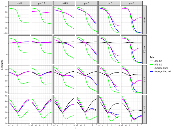
Figure 9: Values of $ATE_{S.1}\left(1;0\right)$ (in black), $ATE_{S.2}\left(1;0\right)$ (in green), the weighted average of Equation (3) (in magenta) and the weighted average of Equation (4) (in blue), under the causal model described in Equation (6).

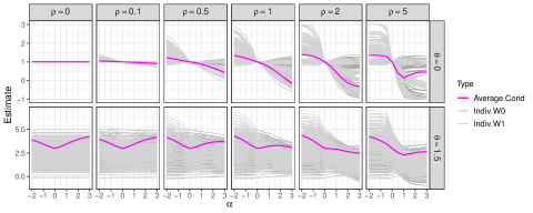
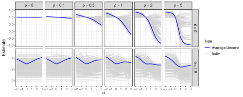
Figure 10: Values of $ATE_{L_{\mid\mathcall{W}=0}}$ (in dark gray), of $ATE_{L_{\mid\mathcall{W}=1}}$ (in gray), for each couple of exposure profiles leading to $\mathcall{X}=1$ and $\mathcall{X}=0$, and of the weighted average (3) (in magenta), under the causal model described in Equation (6).

Figure 11: Values of $ATE_{L}(\bar{x}_{t_{0}};\bar{x}_{t_{0}}^{*})$ (in gray) for each couple of exposure profiles leading to $\mathcall{X}=1$ and $\mathcall{X}=0$, and of the weighted average (4) (in blue), under the causal model described in Equation (6).

Finally, let us turn our attention to the individual causal effects $ATE_{L_{\mid\mathcall{W}=1}}(\bar{x}_{t_{0}};$ $\bar{x}_{t_{0}}^{*})$ and $ATE_{L_{\mid\mathcall{W}=0}}(\bar{x}_{t_{0}};$ $\bar{x}_{t_{0}}^{*})$ and $ATE_{L}\left(\bar{x}_{t_{0}};\bar{x}_{t_{0}}^{*}\right)$ involved in the weighted averages of Equations (3) and (4). Figures 11 and 11 display these individual causal effects for some particular combinations of the parameters of our model. As shown in Figure 11, the values of the individual causal effects $ATE_{L}\left(\bar{x}_{t_{0}};\bar{x}_{t_{0}}^{*}\right)$ are relatively homogeneous for negative values of $\alpha$ and $\rho\leq 2$. In particular, versions of treatment $\mathcall{X}$ are irrelevant and the individual causal effects $ATE_{L}\left(\bar{x}_{t_{0}};\bar{x}_{t_{0}}^{*}\right)$ are all equal when $\theta=0$, $\rho=0$ and/or $\alpha=0$, (in this case, they are also equal to the individual causal effects $ATE_{L_{\mid\mathcall{W}=1}}(\bar{x}_{t_{0}};$ $\bar{x}_{t_{0}}^{*})$, $ATE_{L_{\mid\mathcall{W}=0}}(\bar{x}_{t_{0}};$ $\bar{x}_{t_{0}}^{*})$). The values of the individual causal effects are more heterogeneous for other combinations of the parameters, especially when both $\rho$ and $\alpha$ are large. In these situations, the weighted averages of Equation (4) (and therefore $\widetilde{ATE}_{S.2}(1;0)$ too) and Equation (3) may have to be interpreted with more caution. But again, inspecting the weights involved in these weighted averages is instructive. For example, consider the case where $\theta=0$, $\alpha=3$ and $\rho=5$ in Figure 11. Although the individual terms are very heterogeneous, three of them contribute 96% of the total weights: $ATE_{L}\big{(}{\bf 1}_{5};{\bf 0}_{5}\big{)}\approx-1$, $ATE_{L}\big{(}({\bf 0}_{1},{\bf 1}_{4});{\bf 0}_{5}\big{)}\approx-1$, and $ATE_{L}\big{(}({\bf 1}_{1},{\bf 0}_{1},{\bf 1}_{3});{\bf 0}_{5}\big{)}\approx-1$, with respective weights 0.835, 0.106 and 0.025 (the forth largest weight is only 0.001). In other words, although many different profiles $\bar{x}_{t_{0}}$ and $\bar{x}_{t_{0}}^{*}$ can lead to $\mathcall{X}=1$ and $\mathcall{X}=0$, respectively, and the corresponding causal effects $ATE_{L}(\bar{x}_{t_{0}};$ $\bar{x}_{t_{0}}^{*})$ can be very heterogeneous, mostly one profile (${\bf 0}_{5}$) is observed to lead to $\mathcall{X}=0$ and mostly three profiles (${\bf 1}_{5}$, $({\bf 0}_{1},{\bf 1}_{4})$ and $({\bf 1}_{1},{\bf 0}_{1},{\bf 1}_{3})$) are observed to lead to $\mathcall{X}=1$ in this particular example. Moreover, the three corresponding causal effects $ATE_{L}\big{(}{\bf 1}_{5};{\bf 0}_{5}\big{)}$, $ATE_{L}\big{(}({\bf 0}_{1},{\bf 1}_{4});{\bf 0}_{5}\big{)}$, and $ATE_{L}\big{(}({\bf 1}_{1},{\bf 0}_{1},{\bf 1}_{3});{\bf 0}_{5}\big{)}$ happen to all have very similar values. This can therefore be seen as an example where the weighted average has a relatively clear meaning, and so has $\widetilde{ATE}_{S.2}\left(1;0\right)$, since very little bias was observed when working under the over-simplified model (S.2) in this case; see Figure 9.

5 Discussion

The longitudinal nature of risk factors is often overlooked in epidemiology. In this article, we investigated whether causal effects derived under over-simplified models that ignore the time-varying nature of exposures could still be related to causal effects of potential interest. We focused on the general setting, where the available data concerns summaries $(\mathcall X,\mathcall Z)$ of the full exposure profiles $(\bar{X}_{T},\bar{Z}_{T})$, instead of the full exposure profile themselves, where $\mathcall X$ and $\mathcall Z$ correspond to deterministic functions of $(\bar{X}_{T},\bar{Z}_{T})$. This general framework includes the special case where $\mathcall X=X_{t_{2}}$ and $\mathcall Z=Z_{t_{2}}$, for some time $t_{2}\in\llbracket 1;T\rrbracket$ (e.g., inclusion time in the study). Under the conditions of Theorem 1, the quantity estimated in practice expresses as a weighted average of longitudinal causal effects. But, first, these conditions are very restrictive, and second, even when they are met, the interpretation of the weighted averages is not always straightforward. Therefore, and unsurprisingly, our results are mostly negative, as they state that the quantity estimated in practice when working under over-simplified causal models has generally no clear interpretation in terms of longitudinal causal effects of interest, except under very simple longitudinal causal models.

The bias resulting from this kind of simplification of the true causal model has been less studied and acknowledged than the more standard confounding, collider and selection biases (Greenland,, 2003, Peng and Luke W.,, 2015, Hernán et al.,, 2004, Hernán,, 2010). Overall, our results are consistent with, and complete, a few previous results, which already stressed the need for appropriate statistical methods applied to repeated measurements of exposures when the true causal model is longitudinal, and suggested that overlooking the time-varying nature of exposures would generally lead to unreliable causal effect estimates (Daniel et al.,, 2012, Maxwell and Cole,, 2007, Maxwell et al.,, 2011). Other related works include those on data coarsening, as that of Sofrygin et al., (2019), who empirically showed that while reducing the computational cost of the analyses, partitioning the follow-up into coarse intervals may lead to invalid inference. The study of the impact of the discretization of a continuous-time causal model constitutes an interesting lead for future research.

Just as in the presence of unobserved confounders, we encourage analysts to consider the full DAG representing the causal model rather than the over-simplified one, even when only summary measures, or measures at single time point, are available. This could help them to identify possible biases and not to over-interpret the estimated quantity. This could also be used to develop sensitivity analyses to appreciate the magnitude of the corresponding bias. Moreover, in rare cases, general results on the identifiability of causal effects in the presence of unobserved variables could be applied (Tian and Pearl,, 2002, Shpitser and Pearl,, 2006, Huang and Valtorta,, 2006) to determine whether particular longitudinal causal effects of interest can be identified from the available data. For example, consider the causal model $(L.fd)$ of Figure 12: in this particular case, $ATE_{L}^{(T)}(1;0)=\mathbb{E}_{L}\left(Y^{X_{T}=1}-Y^{X_{T}=0}\right)$ can be identified using the front-door criterion (Pearl, 2009b, ). In other words, $ATE_{L}^{(T)}(1;0)$ can be estimated with data on $X_{T}$, $M_{T}$ and $Y$ only. Conversely, if the analyst focuses on the observed variables only, and works under the simplified model $(S.fd)$, inference would be based on $ATE_{S}^{(T)}(1;0)=\mathbb{E}_{S}\left(Y^{X_{T}=1}-Y^{X_{T}=0}\right)$, which would be identified as $\widetilde{ATE}_{S}^{(T)}(1;0):=\mathbb{E}\left(Y\mid X_{T}=1\right)-\mathbb{E}\left(Y\mid X_{T}=0\right)$. Moreovoer, Theorem 1 applies in this case and ensures that

$$\widetilde{ATE}_{S}^{(T)}(1;0) = \sum_{\begin{subarray}{c}\bar{x}_{T-1}\in\{0,1\}^{T-1}\\ \bar{x}_{T-1*}\in\{0,1\}^{T-1}\end{subarray}}\{ATE_{L}\left((\bar{x}_{T-1},1);(\bar{x}_{T-1}^{*},0)\right)$$

$$\hskip 128.0374pt\times\mathbb{P}(\bar{X}_{T-1}=\bar{x}_{T-1}\mid X_{T}=1)$$

$$\hskip 128.0374pt\times\mathbb{P}(\bar{X}_{T-1}=\bar{x}_{T-1}^{*}\mid X_{T}=0)\}.$$

However, this weighted average differs from $ATE_{L}^{(T)}(1;0)$, and is generally more complicated to interpret (unless some stability assumption holds for example).

(L.fd)

(S.fd)

Figure 12: An example where the front door criterion applies and allows the identification of $ATE_{L}^{(T)}(1;0)=\mathbb{E}_{L}\left(Y^{X_{T}=1}-Y^{X_{T}=0}\right)$. Conversely, the quantity estimated when ignoring the time-varying nature of the exposures, and working under the over-simplified causal model ($S.fd$), usually does not have a clear causal meaning.

A large amount of prospectively collected repeated measures is being made available for a number of exposures through electronic health records and their linkage to biobanks (Beesley et al.,, 2020). However, their analysis raises other challenges, including those pertaining to selection bias (Agniel et al.,, 2018, Beesley and Mukherjee, 2020b, , Winstanley et al.,, 1993, Beesley and Mukherjee, 2020a, ). Prospectively collecting repeated measures of exposures, including biomarkers and -omics data, in well designed cohort studies, as a few studies already did (Kim et al.,, 2017), would be valuable to assess the causal effects of exposures on health-related outcomes.

Disclaimers

Where authors are identified as personnel of the International Agency for Research on Cancer / World Health Organization, the authors alone are responsible for the views expressed in this article and they do not necessarily represent the decisions, policy or views of the International Agency for Research on Cancer / World Health Organization.

Appendices

Appendix A Proof of Theorem 1

Consider a longitudinal model ($L$) and assume that the only available data regarding the exposure of interest consists in $\mathcall X$, which is a deterministic function of $\underline{X}_{t_{1}}^{t_{2}}$, with $1\leq t_{1}\leq t_{2}\leq T$. Let $\mathcall{x}$ and $\mathcall{x}^{*}$, $\mathcall{x}\neq\mathcall{x}^{*}$, be two given possible values of $\mathcall X$, and assume that there exists some $\mathcall{W}\subset\mathcall{Z}$, taking its values in some space $\Omega_{\mathcall{W}}$, such that $0<\mathbb{P}(\mathcall{X}=\mathcall{x}\mid\mathcall{W}=\mathcall{w})<1$ and $0<\mathbb{P}(\mathcall{X}=\mathcall{x}^{*}\mid\mathcall{W}=\mathcall{w})<1$, for all $\mathcall{w}$ such that $\mathbb{P}(\mathcall{W}=\mathcall{w})>0$. Now, consider an over-simplified model ($S$) and assume that $(Y^{\mathcall{X}=\mathcall{x}}\mathbin{\mathchoice{\hbox to0.0pt{\hbox{\set@color$\displaystyle\perp$}\hss}\kern 3.46875pt{}\kern 3.46875pt\hbox{\set@color$\displaystyle\perp$}}{\hbox to0.0pt{\hbox{\set@color$\textstyle\perp$}\hss}\kern 3.46875pt{}\kern 3.46875pt\hbox{\set@color$\textstyle\perp$}}{\hbox to0.0pt{\hbox{\set@color$\scriptstyle\perp$}\hss}\kern 2.36812pt{}\kern 2.36812pt\hbox{\set@color$\scriptstyle\perp$}}{\hbox to0.0pt{\hbox{\set@color$\scriptscriptstyle\perp$}\hss}\kern 1.63437pt{}\kern 1.63437pt\hbox{\set@color$\scriptscriptstyle\perp$}}}\mathcall{X}\mid\mathcall{W})_{S}$. Then, following usual arguments of causal inference (Pearl, 2009a, , Robins,, 1986, Rosenbaum and Rubin,, 1983), the causal effect of interest, $ATE_{S}\left(\mathcall{x};\mathcall{x}^{*}\right):=\mathbb{E}_{S}\left(Y^{\mathcall{X}=\mathcall{x}}-Y^{\mathcall{X}=\mathcall{x}^{*}}\right)$, would be estimated under this over-simplified model $(S)$ as

$$\widetilde{ATE}_{S}\left(\mathcall{x};\mathcall{x}^{*}\right) = \sum_{\mathcall{w}\in\Omega_{\mathcall{W}}}\left[\mathbb{E}\left(Y\mid\mathcall{W}=\mathcall{w},\mathcall{X}=\mathcall{x}\right)-\mathbb{E}\left(Y\mid\mathcall{W}=\mathcall{w},\mathcall{X}=\mathcall{x}^{*}\right)\right]$$

$$\hskip 27.03003pt\times\mathbb{P}(\mathcall{W}=\mathcall{w}).$$

Now assume that there exists some $t_{0}\in\llbracket 1,t_{1}\rrbracket$, some $t_{3}\in\llbracket t_{2},T\rrbracket$, such that $(Y^{\underline{X}_{t_{0}}^{t_{3}}=\underline{x}_{t_{0}}^{t_{3}}}\mathbin{\mathchoice{\hbox to0.0pt{\hbox{\set@color$\displaystyle\perp$}\hss}\kern 3.46875pt{}\kern 3.46875pt\hbox{\set@color$\displaystyle\perp$}}{\hbox to0.0pt{\hbox{\set@color$\textstyle\perp$}\hss}\kern 3.46875pt{}\kern 3.46875pt\hbox{\set@color$\textstyle\perp$}}{\hbox to0.0pt{\hbox{\set@color$\scriptstyle\perp$}\hss}\kern 2.36812pt{}\kern 2.36812pt\hbox{\set@color$\scriptstyle\perp$}}{\hbox to0.0pt{\hbox{\set@color$\scriptscriptstyle\perp$}\hss}\kern 1.63437pt{}\kern 1.63437pt\hbox{\set@color$\scriptscriptstyle\perp$}}}\underline{X}_{t_{0}}^{t_{3}}\mid\mathcall{W})_{L}$. Let $\mathcall{w}$ be any given possible value of $\mathcall{W}$ such that $\mathbb{P}(\mathcall{W}=\mathcall{w})>0$, and $\underline{x}_{t_{0}}^{t_{3}}$ and $\underline{x}_{t_{0}}^{t_{3}*}$ in $\left\{0,1\right\}^{t_{3}-t_{0}+1}$ be any two possible profiles of $\underline{X}_{t_{0}}^{t_{3}}$ leading to $\mathcall{X}=\mathcall{x}$ and $\mathcall{X}=\mathcall{x}^{*}$, respectively, and such that $\mathbb{P}(\underline{X}_{t_{0}}^{t_{3}}=\underline{x}_{t_{0}}^{t_{3}}\mid\mathcall{X}=\mathcall{x},\mathcall{W}=\mathcall{w})>0$ and $\mathbb{P}(\underline{X}_{t_{0}}^{t_{3}}=\underline{x}_{t_{0}}^{t_{3}*}\mid\mathcall{X}=\mathcall{x}^{*},\mathcall{W}=\mathcall{w})>0$. It follows that $\mathbb{P}(\underline{X}_{t_{0}}^{t_{3}}=\underline{x}_{t_{0}}^{t_{3}}\mid\mathcall{W}=\mathcall{w})>0$ and $\mathbb{P}(\underline{X}_{t_{0}}^{t_{3}}=\underline{x}_{t_{0}}^{t_{3}*}\mid\mathcall{W}=\mathcall{w})>0$. Next, usual arguments of causal inference (Pearl, 2009a, , Robins,, 1986, Rosenbaum and Rubin,, 1983) yield

$$ATE_{L_{\mid\mathcall{W}=\mathcall{w}}}\left(\underline{x}_{t_{0}}^{t_{3}};\underline{x}^{t_{3}*}_{t_{0}}\right) = \sum_{\mathcall{w}\in\Omega_{\mathcall{W}}}\mathbb{E}_{L}\left(Y^{\underline{X}_{t_{0}}^{t_{3}}=\underline{x}_{t_{0}}^{t_{3}}}-Y^{\underline{X}_{t_{0}}^{t_{3}}=\underline{x}^{t_{3}*}_{t_{0}}}\mid\mathcall{W}=\mathcall{w}\right),$$

$$= \sum_{\mathcall{w}\in\Omega_{\mathcall{W}}}\Big{[}\mathbb{E}_{L}\Big{(}Y^{\underline{X}_{t_{0}}^{t_{3}}=\underline{x}_{t_{0}}^{t_{3}}}\mid\mathcall{W}=\mathcall{w},{\underline{X}_{t_{0}}^{t_{3}}=\underline{x}_{t_{0}}^{t_{3}}}\Big{)}$$

$$\hskip 29.87547pt-\mathbb{E}_{L}\Big{(}Y^{\underline{X}_{t_{0}}^{t_{3}}=\underline{x}^{t_{3}*}_{t_{0}}}\mid\mathcall{W}=\mathcall{w},{\underline{X}_{t_{0}}^{t_{3}}=\underline{x}^{t_{3}*}_{t_{0}}}\Big{)}\Big{]},$$

$$= \sum_{\mathcall{w}\in\Omega_{\mathcall{W}}}\Big{[}\mathbb{E}\Big{(}Y\mid\mathcall{W}=\mathcall{w},{\underline{X}_{t_{0}}^{t_{3}}=\underline{x}_{t_{0}}^{t_{3}}}\Big{)}-\mathbb{E}\Big{(}Y\mid\mathcall{W}=\mathcall{w},{\underline{X}_{t_{0}}^{t_{3}}=\underline{x}^{t_{3}*}_{t_{0}}}\Big{)}\Big{]}.$$

Because $\underline{X}_{t_{0}}^{t_{3}}$ d-separates $\mathcall{X}$ and $\mathcall{W}$ under model ($L$) (Pearl, 2009b, , Verma and Pearl,, 1988), we have, for any any $\mathcall{w}$ in $\Omega_{\mathcall{W}}$ and any $\underline{x}_{t_{0}}^{t_{3}}$ in $\{0,1\}^{t_{3}-t_{0}+1}$ such that $\mathbb{P}(\underline{X}_{t_{0}}^{t_{3}}=\underline{x}_{t_{0}}^{t_{3}}\mid\mathcall{W}=\mathcall{w})>0$,

$$\mathbb{E}\Big{(}Y\mid\mathcall{W}=\mathcall{w},{\underline{X}_{t_{0}}^{t_{3}}=\underline{x}_{t_{0}}^{t_{3}}}\Big{)} = \mathbb{E}\Big{(}Y\mid\mathcall{W}=\mathcall{w},\mathcall{X}=\mathcall{x},{\underline{X}_{t_{0}}^{t_{3}}=\underline{x}_{t_{0}}^{t_{3}}}\Big{)},$$

with $\mathcall{x}$ corresponding to the value taken by $\mathcall{X}$ when $\underline{X}_{t_{0}}^{t_{3}}=\underline{x}_{t_{0}}^{t_{3}}$. In other respect, we have

$$\mathbb{E}\left(Y\mid\mathcall{W}=\mathcall{w},\mathcall{X}=\mathcall{x}\right) = \sum_{\underline{x}_{t_{0}}^{t_{3}}\in\left\{0,1\right\}^{t_{3}-t_{0}+1}}\mathbb{E}\left(Y\mid\mathcall{W}=\mathcall{w},\mathcall{X}=\mathcall{x},{\underline{X}_{t_{0}}^{t_{3}}=\underline{x}_{t_{0}}^{t_{3}}}\right)$$

$$\hskip 78.24507pt\times\mathbb{P}(\underline{X}_{t_{0}}^{t_{3}}=\underline{x}_{t_{0}}^{t_{3}}\mid\mathcall{W}=\mathcall{w},\mathcall{X}=\mathcall{x}),$$

$$= \sum_{\underline{x}_{t_{0}}^{t_{3}}\in\left\{0,1\right\}^{t_{3}-t_{0}+1}}\mathbb{E}\left(Y\mid\mathcall{W}=\mathcall{w},{\underline{X}_{t_{0}}^{t_{3}}=\underline{x}_{t_{0}}^{t_{3}}}\right)$$

$$\hskip 78.24507pt\times\mathbb{P}(\underline{X}_{t_{0}}^{t_{3}}=\underline{x}_{t_{0}}^{t_{3}}\mid\mathcall{W}=\mathcall{w},\mathcall{X}=\mathcall{x}),$$

$$= \sum_{\underline{x}_{t_{0}}^{t_{3}}\in\left\{0,1\right\}^{t_{3}-t_{0}+1}}\mathbb{E}_{L}\Big{(}Y^{\underline{X}_{t_{0}}^{t_{3}}=\underline{x}_{t_{0}}^{t_{3}}}\mid\mathcall{W}=\mathcall{w}\Big{)}$$

$$\hskip 78.24507pt\times\mathbb{P}(\underline{X}_{t_{0}}^{t_{3}}=\underline{x}_{t_{0}}^{t_{3}}\mid\mathcall{W}=\mathcall{w},\mathcall{X}=\mathcall{x}),$$

where the second equality comes from the fact that $\underline{X}_{t_{0}}^{t_{3}}=\underline{x}_{t_{0}}^{t_{3}}\Rightarrow\mathcall{X}=\mathcall{x}$, for any $\underline{x}_{t_{0}}^{t_{3}}$ such that $\mathbb{P}(\underline{X}_{t_{0}}^{t_{3}}=\underline{x}_{t_{0}}^{t_{3}}\mid\mathcall{W}=\mathcall{w},\mathcall{X}=\mathcall{x})\neq 0$. This finally yields

$$\widetilde{ATE}_{S}(\mathcall{x};\mathcall{x}^{*}) = \sum_{\mathcall{w}\in\Omega_{\mathcall{W}}}\sum_{\begin{subarray}{c}\underline{x}_{t_{0}}^{t_{3}},\\ \underline{x}^{t_{3}*}_{t_{0}}\in\left\{0,1\right\}^{t_{3}-t_{0}+1}\end{subarray}}\{ATE_{L_{\mid\mathcall{W}=\mathcall{w}}}\left(\underline{x}_{t_{0}}^{t_{3}};\underline{x}^{t_{3}*}_{t_{0}}\right)\times\mathbb{P}(\underline{X}_{t_{0}}^{t_{3}}=\underline{x}_{t_{0}}^{t_{3}}\mid\mathcall{X}=\mathcall{x},\mathcall{W}=\mathcall{w})$$

$$\hskip 153.6447pt\times\mathbb{P}(\underline{X}_{t_{0}}^{t_{3}}=\underline{x}_{t_{0}}^{t_{3}*}\mid\mathcall{X}=\mathcall{x}^{*},\mathcall{W}=\mathcall{w})$$

$$\hskip 153.6447pt\times\mathbb{P}(\mathcall{W}=\mathcall{w})\},$$

where the sums are over all $\bar{x}_{t_{0}}^{t_{3}}$ and $\bar{x}_{t_{0}}^{t_{3}*}$ in $\{0,1\}^{t_{3}-t_{0}+1}$ such that $\mathbb{P}(\underline{X}_{t_{0}}^{t_{3}}=\underline{x}_{t_{0}}^{t_{3}}\mid\mathcall{W}=\mathcall{w},\mathcall{X}=\mathcall{x})$ and $\mathbb{P}(\underline{X}_{t_{0}}^{t_{3}}=\underline{x}_{t_{0}}^{t_{3}*}\mid\mathcall{W}=\mathcall{w},\mathcall{X}=\mathcall{x}^{*})$, respectively, are not null.

The proof of the result under condition ($T.Uncond$) follows from similar, but simpler, arguments and is therefore omitted.

References

- Aalen et al., (2016) Aalen, O., Røysland, K., Gran, J., Kouyos, R., and Lange, T. (2016). Can we believe the dags? a comment on the relationship between causal dags and mechanisms. Statistical Methods in Medical Research, 25(5):2294–2314. PMID: 24463886.
- Agniel et al., (2018) Agniel, D., Kohane, I. S., and Weber, G. M. (2018). Biases in electronic health record data due to processes within the healthcare system: retrospective observational study. BMJ, 361.
- Agudo et al., (2012) Agudo, A., Bonet, C., Travier, N., González, C., Vineis, P., Bueno-de Mesquita, H., Trichopoulos, D., Boffetta, P., Clavel-Chapelon, F., Boutron-Ruault, M.-C., Kaaks, R., Lukanova, A., Schütze, M., Boeing, H., Tjønneland, A., Halkjær, J., Overvad, K., Dahm, C., Quirós, J., and Riboli, E. (2012). Impact of cigarette smoking on cancer risk in the european prospective investigation into cancer and nutrition study. Journal of Clinical Oncology, pages 4550–4557.
- Arnold et al., (2019) Arnold, M., Charvat, H., Freisling, H., Noh, H., Adami, H.-O., Soerjomataram, I., and Weiderpass, E. (2019). Adulthood overweight and survival from breast and colorectal cancer in swedish women. Cancer Epidemiology and Prevention Biomarkers.
- Arnold et al., (2016) Arnold, M., Freisling, H., Stolzenberg-Solomon, R., Kee, F., O’Doherty, M., Ordóẽz Mena, J. M., Wilsgaard, T., May, A., Bueno-de Mesquita, H., Tjønneland, A., Orfanos, P., Trichopoulou, A., Boffetta, P., Bray, F., Jenab, M., and Soerjomataram, I. (2016). Overweight duration in older adults and cancer risk: a study of cohorts in europe and the united states. European Journal of Epidemiology, 31(9):893–904.
- Bagnardi et al., (2015) Bagnardi, V., Rota, M., Botteri, E., Tramacere, I., Islami, F., Fedirko, V., Scotti, L., Jenab, M., Turati, F., Pasquali, E., Pelucchi, C., Galeone, C., Bellocco, R., Negri, E., Corrao, G., Boffetta, P., and Vecchia, C. (2015). Alcohol consumption and site-specific cancer risk: a comprehensive dose-response meta-analysis. British Journal of Cancer, 112(3):580–593.
- (7) Beesley, L. and Mukherjee, B. (2020a). Statistical inference for association studies using electronic health records: handling both selection bias and outcome misclassification. Biometrics.
- (8) Beesley, L. J. and Mukherjee, B. (2020b). Bias reduction and inference for electronic health record data under selection and phenotype misclassification: three case studies. medRxiv.
- Beesley et al., (2020) Beesley, L. J., Salvatore, M., Fritsche, L. G., Pandit, A., Rao, A., Brummett, C., Willer, C. J., Lisabeth, L. D., and Mukherjee, B. (2020). The emerging landscape of health research based on biobanks linked to electronic health records: Existing resources, statistical challenges, and potential opportunities. Statistics in Medicine, 39(6):773–800.
- Bradbury et al., (2019) Bradbury, K. E., Appleby, P. N., Tipper, S. J., Travis, R. C., Allen, N. E., Kvaskoff, M., Overvad, K., Tjønneland, A., Halkjær, J., Cervenka, I., et al. (2019). Circulating insulin-like growth factor i in relation to melanoma risk in the european prospective investigation into cancer and nutrition. International journal of cancer, 144(5):957–966.
- Chan et al., (2011) Chan, A. T., Ogino, S., Giovannucci, E. L., and Fuchs, C. S. (2011). Inflammatory markers are associated with risk of colorectal cancer and chemopreventive response to anti-inflammatory drugs. Gastroenterology, 140(3):799–808.
- Daniel et al., (2012) Daniel, R. M., Cousens, S., B. L., DE Stavola, B., Kenward, M. G., and Sterne, J. A. (2012). Methods for dealing with time-dependent confounding. Statistics in Medicine, 32:1584–1618.
- De Rubeis et al., (2019) De Rubeis, V., Cotterchio, M., Smith, B. T., Griffith, L. E., Borgida, A., Gallinger, S., Cleary, S., and Anderson, L. N. (2019). Trajectories of body mass index, from adolescence to older adulthood, and pancreatic cancer risk; a population-based case–control study in ontario, canada”. Cancer Causes Control, 30(9):955–966.
- Dossus et al., (2013) Dossus, L., Lukanova, A., Rinaldi, S., Allen, N., Cust, A. E., Becker, S., Tjonneland, A., Hansen, L., Overvad, K., Chabbert-Buffet, N., et al. (2013). Hormonal, metabolic, and inflammatory profiles and endometrial cancer risk within the epic cohort—a factor analysis. American journal of epidemiology, 177(8):787–799.
- Fan et al., (2008) Fan, A. Z., Russell, M., Stranges, S., Dorn, J., and Trevisan, M. (2008). Association of Lifetime Alcohol Drinking Trajectories with Cardiometabolic Risk. The Journal of Clinical Endocrinology & Metabolism, 93(1):154–161.
- Greenland, (2003) Greenland, S. (2003). Quantifying biases in causal models: classical confounding vs collider-stratification bias. Epidemiology (Cambridge, Mass.), 14(3):300-306.
- Hernan and Robins, (2020) Hernan, M. A. and Robins, J. M. (2020). Causal Inference: What If. Boca Raton: Chapman Hall/CRC. forthcoming.
- Hernan and VanderWeele, (2011) Hernan, M. A. and VanderWeele, T. J. (2011). Compound treatments and transportability of causal inference. Epidemiology, 22(3):368 – 377.
- Hernán, (2010) Hernán, M. (2010). The hazards of hazard ratios. Epidemiology (Cambridge, Mass.), 21:13–5.
- Hernán et al., (2004) Hernán, M., Hernández-DÃaz, S., and Robins, J. (2004). A structural approach to selection bias. Epidemiology (Cambridge, Mass.), 15:615–25.
- Huang and Valtorta, (2006) Huang, Y. and Valtorta, M. (2006). Identifiability in causal bayesian networks: A sound and complete algorithm. In In:Proceedings of the twenty-first national conference on artificial intelligence (AAAI 2006). AAAI Press, Menlo Park, CA.
- Kim et al., (2017) Kim, Y., Han, B., and group, K. (2017). Cohort profile: The korean genome and epidemiology study (koges) consortium. International Journal of Epidemiology, e20:1–10.
- Kunzmann et al., (2018) Kunzmann, A. T., Coleman, H. G., Huang, W.-Y., and Berndt, S. I. (2018). The association of lifetime alcohol use with mortality and cancer risk in older adults: A cohort study. PLOS Medicine, 15:1–18.
- Lauby-Secretan et al., (2016) Lauby-Secretan, B., Scoccianti, C., Loomis, D., Grosse, Y., Bianchini, F., and Straif, K. (2016). Body fatness and cancer - viewpoint of the iarc working group. New England Journal of Medicine, 375(8):794–798.
- Maxwell and Cole, (2007) Maxwell, S. E. and Cole, D. A. (2007). Bias in cross-sectional analyses of longitudinal mediation. Psychological Methods, 12:23–44.
- Maxwell et al., (2011) Maxwell, S. E., Cole, D. A., and Mitchell, M. A. (2011). Bias in cross-sectional analyses of longitudinal mediation: Partial and complete mediation under an autoregressive model. Multivariate Behavioral Research, 46(11):816–841.
- (27) Pearl, J. (2009a). Causal inference in statistics: An overview. Statistics Surveys, 3:96–146.
- (28) Pearl, J. (2009b). Causality: Models, Reasoning, and Inference. Cambridge University Press, New York.
- Peng and Luke W., (2015) Peng, D. and Luke W., M. (2015). To adjust or not to adjust? sensitivity analysis of m-bias and butterfly-bias. Journal of Causal Inference, 3(1):41–57.
- Platt et al., (2010) Platt, A., Sloan, F., and Costanzo, P. (2010). Alcohol-consumption trajectories and associated characteristics among adults older than age 50*. Journal of studies on alcohol and drugs, 71:169–79.
- Robins, (1986) Robins, J. (1986). A new approach to causal inference in mortality studies with a sustained exposure period-application to control of the healthy worker survivor effect. Mathematical Modelling, 7(9):1393 – 1512.
- Rosenbaum and Rubin, (1983) Rosenbaum, P. R. and Rubin, D. B. (1983). The central role of the propensity score in observational studies for causal effects. Biometrika, 70(1):41–55.
- Shpitser and Pearl, (2006) Shpitser, I. and Pearl, J. (2006). Identification of joint interventional distributions in recursive semi-markovian causal models. In In: Proceedings of the 21st national conference on artificial intelligence and the 18th innovative applications of artificial intelligence conference (AAAI 2006). AAAI Press, Menlo Park, CA, volume 2.
- Sofrygin et al., (2019) Sofrygin, O., Zhu, Z., Schmittdiel, J. A., Adams, A. S., Grant, R. W., van der Laan, M. J., and Neugebauer, R. (2019). Targeted learning with daily ehr data. Statistics in Medicine, 38(16):3073–3090.
- Tian and Pearl, (2002) Tian, J. and Pearl, J. (2002). A general identification condition for causal effects. Proceedings of the Eighteenth National Conference on Artificial Intelligence.
- Tian and Pearl, (2003) Tian, J. and Pearl, J. (2003). On the identification of causal effects. In Technical report, cognitive systems laboratory, LosAngeles: University of California.
- VanderWeele, (2015) VanderWeele, T. J. (2015). Explanation in Causal Inference - Methods for Mediation and Interaction. Oxford.
- VanderWeele and Hernan, (2013) VanderWeele, T. J. and Hernan, M. A. (2013). Causal inference under multiple versions of treatment. Journal of Causal Inference, 1:1 – 20.
- VanderWeele and Tchetgen Tchetgen, (2017) VanderWeele, T. J. and Tchetgen Tchetgen, E. (2017). Mediation analysis with time-varying exposures and mediators. Journal of the Royal Statistical Society: Series B (Statistical Methodology), 79:917–938.
- Verma and Pearl, (1988) Verma, T. and Pearl, J. (1988). Causal networks: Semantics and expressiveness. Proceedings of the Fourth Workshop on Uncertainty in Artificial Intelligence.
- Winstanley et al., (1993) Winstanley, T., Limb, D., Wheat, P., and Nicol, C. (1993). Multipoint identification of enterobacteriaceae: report of the british society for microbial technology collaborative study. Journal of clinical pathology, 46(7):637-641.
- Yang et al., (2019) Yang, Y., Dugu,́ P.-A., Lynch, B. M., Hodge, A. M., Karahalios, A., MacInnis, R. J., Milne, R. L., Giles, G. G., and English, D. R. (2019). Trajectories of body mass index in adulthood and all-cause and cause-specific mortality in the melbourne collaborative cohort study. BMJ Open, 9(8).
- Zheng et al., (2018) Zheng, R., Du, M., Zhang, B., Xin, J., Chu, H., Ni, M., Zhang, Z., Gu, D., and Wang, M. (2018). Body mass index (bmi) trajectories and risk of colorectal cancer in the plco cohort. In British Journal of Cancer.