Nondegenerate solitons in Manakov system

Abstract

It is known that Manakov equation which describes wave propagation in two mode optical fibers, photorefractive materials, etc. can admit solitons which allow energy redistribution between the modes on collision that also leads to logical computing. In this paper, we point out that Manakov system can admit more general type of nondegenerate fundamental solitons corresponding to different wave numbers, which undergo collisions without any energy redistribution. The previously known class of solitons which allows energy redistribution among the modes turns out to be a special case corresponding to solitary waves with identical wave numbers in both the modes and travelling with the same velocity. We trace out the reason behind such a possibility and analyze the physical consequences.

Discovery of solitons has created a new pathway to understand the wave propagation in many physical systems with nonlinearity a . In particular, the existence of optical solitons in nonlinear Kerr media b provoked the investigation on solitons from different perspectives, particularly from applications point of view. By generalizing the waves propagating in an isotropic medium c to an anisotropic medium, a pair of coupled equations for orthogonally polarized waves has been obtained by Manakov d ; d1 as

$$iq_{jz}+q_{jtt}+2\sum_{p=1}^{2}|q_{p}|^{2}q_{j}=0,~{}~{}~{}~{}j=1,2$$ (1)

where $q_{j}$, $j=1,2$, describe orthogonally polarized complex waves. Here the subscripts $z$ and $t$ represent normalized distance and retarded time, respectively. Equation (1) also appears in many physical situations such as single optical field propagation in birefringent fibers e , self trapped incoherent light beam propagation in photorefractive medium f ; g ; h and so on. Generalization of Eq. (1) to arbitrary $N$-waves is useful to model optical pulse propagation in multi-mode fibers i . It has been identified d that the polarization vectors of the solitons change when orthogonally polarized waves nonlinearly interact with each other leading to energy exchange interaction between the modes j . Experimental observation of the latter has been demonstrated in k ; l ; l11 . The shape changing collision property of such waves, which we designate here as degenerate polarized soliton propagating with identical velocity and wave number in the two modes, gave rise to the possibility of constructing logic gates leading to all optical computing atleast in a theoretical sense l1 ; m ; ma . Energy sharing collisions among the optical vector solitons has been explored m by constructing multi-soliton solutions explicitly to the multi-component nonlinear Schrödinger equations. Further, it has been shown that the multi-soliton interaction process satisfies Yang-Baxter relation m1 . It is clear from these studies that the shape changing collision that occurs among the solitons with identical wave numbers in all the modes has been well understood. However, to our knowledge, studies on solitons with non-identical wave numbers in all the modes have not been considered so far. Consequently one would like to explore the role of such additional wave number(s) on the soliton structures and collision scenario as well.

In the contemporary studies, a new class of multi-hump solitons has been identified in different physical situations. In birefringent dispersive nonlinear media, asymmetric double hump-single hump frozen states have been obtained n . Double hump structure has been observed for the Manakov equation by considering two soliton solutions o ; p . The first experimental observation of multi-hump solitons was demonstrated when the self trapped incoherent wave packets propagate in a dispersive nonlinear medium q . These unusual solitons have been found in various nonlinear coupled field models t . Stability of multi-hump optical solitons has also been investigated in the case of saturable nonlinear medium u . It is reported that in such a medium both two and three hump solitons do not survive after collision. $N$-self trapped multi-humped partially coherent solitons have also been explored in photorefractive medium v . The coherent coupling between copropagating fields also give rise to double hump solitons in the coherently coupled nonlinear Schrödinger system w1 . In addition to the above, the dynamics of multi-hump structured solitons have also been studied in certain dissipative systems new1 ; new2 ; new2a ; new2b . A double hump phase-locked higher-order vector soliton has been observed and its dynamics has been investigated in mode-locked fiber lasers new1 ; new2 . Similarly in deployed fiber systems and fiber laser cavities, double hump solitons have been observed during the buildup process of soliton molecules new3 ; new4 .

Motivated by the above, in this letter we present a new class of generalized soliton solutions for the Manakov model, exhibiting various interesting structures under general parametric conditions. A fundamental double hump soliton (as well as other structures described below) sustains its shape even after collision with another similar soliton. This behaviour is in contrast to the one which exists in saturable nonlinear media where two and three humps do not survive after collision. The soliton solutions presented in this letter also have both symmetric and asymmetric natures analogous to the partially coherent solitons in photorefractive medium. Under specific parametric restriction on wave numbers they degenerate into the standard Manakov solitons exhibiting shape changing collisions j ; m .

To explore the new family of soliton solutions for Eq. (1), we consider the bilinear forms of Eq. (1) as $(iD_{z}+D^{2}_{t})g^{(j)}\cdot f=0$, $j=1,2$, and $D^{2}_{t}f\cdot f=2\sum_{n=1}^{2}g^{(n)}g^{(n)*}$, which are obtained through the dependent variable transformations, $q_{j}=g^{(j)}/f$, $j=1,2$. Here $D_{z}$ and $D_{t}$ are the well known Hirota bilinear operators wa , $g^{(j)}(z,t)$ are complex functions whereas $f$ is a real function and $*$ denotes complex conjugation. In principle, multi-soliton solutions of Eq. (1) can be constructed by solving recursively the system of linear partial differential equations which results in by substituting the series expansions $g^{(j)}=\epsilon g_{1}^{(j)}+\epsilon^{3}g_{3}^{(j)}+...$ and $f=1+\epsilon^{2}f_{2}+\epsilon^{4}f_{4}+...$ for the unknown functions $g^{(j)}$ and $f$ in the bilinear forms. Here $\epsilon$ is a formal expansion parameter.

Considering two different seed solutions for $g_{1}^{(1)}$ and $g_{1}^{(2)}$ as $\alpha_{1}^{(1)}e^{\eta_{1}}$ and $\alpha_{1}^{(2)}e^{\xi_{1}}$, respectively, where $\eta_{1}=k_{1}t+ik_{1}^{2}z$, $\xi_{1}=l_{1}t+il_{1}^{2}z$, and $\alpha_{1}^{(j)}$, $j=1,2$, $k_{1}$ and $l_{1}$ are in general independent complex wave numbers, to the resultant linear partial differential equations $(iD_{z}+D^{2}_{t})g^{(j)}_{1}\cdot 1=0$, $j=1,2$, which arise in the lowest order of $\epsilon$, the series expansion gets terminated as $g^{(j)}=\epsilon g_{1}^{(j)}+\epsilon^{3}g_{3}^{(j)}$  and   $f=1+\epsilon^{2}f_{2}+\epsilon^{4}f_{4}$. The explicit forms of the unknown functions present in the truncated series expansions constitute a new fundamental one soliton solution to Eq. (1) in the form

$$q_{1}=(\alpha_{1}^{(1)}e^{\eta_{1}}+e^{\eta_{1}+\xi_{1}+\xi_{1}^{*}+\Delta_{1}^{(1)}})/D_{1}$$

$$q_{2}=(\alpha_{1}^{(2)}e^{\xi_{1}}+e^{\eta_{1}+\eta_{1}^{*}+\xi_{1}+\Delta_{1}^{(2)}})/D_{1},$$ (2)

where $D_{1}=1+e^{\eta_{1}+\eta_{1}^{*}+\delta_{1}}+e^{\xi_{1}+\xi_{1}^{*}+\delta_{2}}+e^{\eta_{1}+\eta_{1}^{*}+\xi_{1}+\xi_{1}^{*}+\delta_{11}}$, $e^{\delta_{1}}=\frac{|\alpha_{1}^{(1)}|^{2}}{(k_{1}+k_{1}^{*})^{2}}$, $e^{\delta_{2}}=\frac{|\alpha_{1}^{(2)}|^{2}}{(l_{1}+l_{1}^{*})^{2}}$, $e^{\delta_{11}}=\frac{|k_{1}-l_{1}|^{2}|\alpha_{1}^{(1)}|^{2}|\alpha_{1}^{(2)}|^{2}}{(k_{1}+k_{1}^{*})^{2}(k_{1}^{*}+l_{1})(k_{1}+l_{1}^{*})(l_{1}+l_{1}^{*})^{2}}$, $e^{\Delta_{1}^{(1)}}=\frac{(k_{1}-l_{1})\alpha_{1}^{(1)}|\alpha_{1}^{(2)}|^{2}}{(k_{1}+l_{1}^{*})(l_{1}+l_{1}^{*})^{2}}$, $e^{\Delta_{1}^{(2)}}=-\frac{(k_{1}-l_{1})|\alpha_{1}^{(1)}|^{2}\alpha_{1}^{(2)}}{(k_{1}+k_{1}^{*})^{2}(k_{1}^{*}+l_{1})}$.

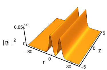
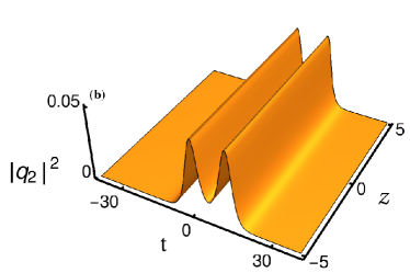
Figure 1: Nondegenerate symmetric double hump one-soliton in the two modes: (a) and (b) denote the intensities of the components $q_{1}$ and $q_{2}$, respectively. The parameters are chosen as $k_{1}=0.316+0.5i$, $l_{1}=0.333+0.5i$, $\alpha_{1}^{(1)}=0.49+0.45i$ and $\alpha_{1}^{(2)}=0.45+0.45i$.

From the above, it is evident that the fundamental solitons propagating in the two modes are characterized by four arbitrary complex parameters $k_{1},l_{1}$ and $\alpha_{1}^{(j)},j=1,2$. These nontrivial parameters determine the shape, amplitude, width and velocity of the solitons which propagate in the Kerr media or photorefractive media. The amplitudes of the solitons that are present in the two modes $q_{1}$ and $q_{2}$ are governed by the real parts of the wave numbers $k_{1}$ and $l_{1}$ whereas velocities are described by the imaginary parts of them. Note that $\alpha_{1}^{(j)}$, $j=1,2$, are related to the unit polarization vectors of the solitons in the two modes.

To identify certain special features of the obtained four complex parameter family of soliton solution (2) we first consider (for simplicity of analysis) the special case where the imaginary parts of the wave numbers $k_{1I}=l_{1I}$ but with $k_{1R}\neq l_{1R}$. The latter case yields atleast the following four different symmetric wave profiles, apart from similar asymmetric wave profiles, from solution (2) by incorporating the condition $k_{1R}<l_{1R}$ with further conditions and with suitable choices of parameters (examples given in w2 ): (i) single hump-single hump soliton: $\alpha_{1R}^{(1)}>\alpha_{1R}^{(2)}$ and $\alpha_{1I}^{(1)}=\alpha_{1I}^{(2)}$, (ii) double hump-single hump soliton: $\alpha_{1R}^{(1)}=\alpha_{1R}^{(2)}$ and $\alpha_{1I}^{(1)}<\alpha_{1I}^{(2)}$, (iii) double hump-flat top soliton: $\alpha_{1R}^{(1)}=\alpha_{1R}^{(2)}$ and $\alpha_{1I}^{(1)}\approx\alpha_{1I}^{(2)}$, (iv) double hump-double hump soliton: $\alpha_{1R}^{(1)}>\alpha_{1R}^{(2)}$ and $\alpha_{1I}^{(1)}=\alpha_{1I}^{(2)}$. Similar conditions can be given for $k_{1R}>l_{1R}$ also. We have not listed the asymmetric wave profiles here for brevity, which also exhibit the properties discussed below. Similar classification can be made for the case $k_{1I}\neq l_{1I}$, so that the solitons propagate in the two modes with different velocities, and exhibit similar interaction properties. These will be discussed separately.

To illustrate the symmetric case, we display only the intensity profile of the double hump soliton in Fig. 1. We call the solitons that have two distinct wave numbers in both the modes as in Eq. (2) as nondegenerate solitons (which can exist as different profiles as described above) while the solitons which have identical wave numbers in all the modes (which exist only in single hump form) are designated as degenerate solitons. In particular, in the special case when $k_{1}=l_{1}$, the forms of $q_{j}$ given in Eq. (2) degenerate into the standard bright soliton form d ; j

$$q_{j}=\frac{\alpha_{1}^{(j)}e^{\eta_{1}}}{1+e^{\eta_{1}+\eta_{1}^{*}+R}},~{}j=1,2,\\$$ (3)

which can be rewritten as

$$q_{j}=k_{1R}\hat{A_{j}}e^{i\eta_{1I}}\mbox{sech}(\eta_{1R}+\frac{R}{2}),$$ (4)

where $\eta_{1R}=k_{1R}(t-2k_{1I}z)$, $\eta_{1I}=k_{1I}t+(k_{1R}^{2}-k_{1I}^{2})z$, $\hat{A_{j}}=\frac{\alpha_{1}^{(j)}}{\sqrt{(|\alpha_{1}^{(1)}|^{2}+|\alpha_{1}^{(2)}|^{2})}}$, $e^{R}=\frac{(|\alpha_{1}^{(1)}|^{2}+|\alpha_{1}^{(2)}|^{2})}{(k_{1}+k_{1}^{*})^{2}}$, $j=1,2$. Note that the above fundamental bright soliton always propagates in both the modes $q_{1}$ and $q_{2}$ with the same velocity $2k_{1I}$. The polarization vectors $(\hat{A}_{1},\hat{A}_{2})^{\dagger}$ have different amplitudes and phases, unlike the case of nondegenerate case where they have only different phases $(A_{1}=(\frac{\alpha_{1}^{(1)}}{\alpha_{1}^{(1)*}})^{\frac{1}{2}},A_{2}=(\frac{\alpha_{1}^{(2)}}{\alpha_{1}^{(2)*}})^{\frac{1}{2}})^{\dagger}$ (vide Eq. (2)), but same unit amplitude. We call the above type of soliton (3) or (4) as degenerate soliton w11 .

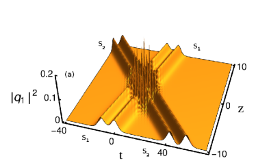
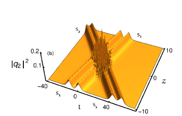
Figure 2: Nondegenerate solitons exhibiting shape preserving collisions: (a) and (b) denote the elastic collision of two symmetric double hump solitons for the parametric values $k_{1}=0.333+0.5i$, $k_{2}=0.3-2.2i$, $l_{1}=0.3+0.5i$, $l_{2}=0.333-2.2i$, $\alpha_{1}^{(1)}=0.45+0.45i$, $\alpha_{2}^{(1)}=0.49+0.45i$, $\alpha_{1}^{(2)}=0.49+0.45i$ and $\alpha_{2}^{(2)}=0.45+0.45i$.

In order to understand the collision dynamics of the soliton solution of the kind (2), it is essential to construct the corresponding two soliton solution. In the latter case, the series expansion for $q_{j}$, $j=1,2$, gets terminated as $g^{(j)}=\epsilon g_{1}^{(j)}+\epsilon^{3}g_{3}^{(j)}+\epsilon^{5}g_{5}^{(j)}+\epsilon^{7}g_{7}^{(j)}$ and $f=1+\epsilon^{2}f_{2}+\epsilon^{4}f_{4}+\epsilon^{6}f_{6}+\epsilon^{8}f_{8}$. The obtained explicit forms of $g^{(j)}$ and $f$, $j=1,2$, in the above truncated expansions constitute the nondegenerate two soliton solution of Eq. (1), which reduces to the known form given in Ref. j for $k_{i}=l_{i}$, $i=1,2$. The complicated profiles of the present nondegenerate two soliton solution are governed by eight arbitrary complex parameters $k_{j}$, $l_{j}$, $\alpha_{1}^{(j)}$ and $\alpha_{2}^{(j)}$, $j=1,2$ (see supplemental material w2 ).

To study the collision dynamics between the nondegenerate two solitons, as an example, we again confine ourselves to the case of symmetric double hump solitons by fixing the imaginary parts of the wave numbers as $k_{iI}=l_{iI}$, $i=1,2$. For other types also similar analysis has been carried out. By carefully examining the behavior of the obtained nondegenerate two soliton solution in the asymptotic regimes, $z\rightarrow\pm\infty$, we find that the phases of the fundamental nondegenerate double hump solitons in both the modes change during the collision process, while the intensities remain unchanged. This can be verified by defining the transition amplitudes as $T_{j}^{l}$ $=$ $\frac{A_{j}^{l+}}{A_{j}^{l-}}$ , $j$ $=$1,2 and $l=1,2$, where subscript $j$ represents the mode and superscript $l\pm$ denote the nondegenerate soliton numbers 1 and 2 designated as $S_{1}$ and $S_{2}$, respectively, in the asymptotic regimes $z\rightarrow\pm\infty$.

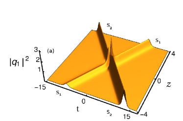
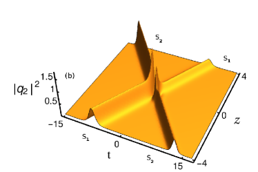
Figure 3: Degenerate solitons exhibiting shape changing collision: (a) and (b) denote the energy sharing collision in the two modes for the parametric values $k_{1}=l_{1}=1+i$, $k_{2}=l_{2}=1.51-1.5i$, $\alpha_{1}^{(1)}=0.5+0.5i$, $\alpha_{2}^{(1)}=\alpha_{1}^{(2)}=\alpha_{2}^{(2)}=1$.

In the nondegenerate double hump soliton case, the amplitudes of the solitons $S_{1}$ and $S_{2}$ in the first mode $\big{(}2k_{1R}A_{1}^{1-}$, $\frac{(k_{1}-k_{2})(k_{2}-l_{1})^{1/2}(k_{1}+k_{2}^{*})(k_{2}^{*}+l_{1})^{1/2}}{(k_{1}^{*}-k_{2}^{*})(k_{2}^{*}-l_{1}^{*})^{1/2}(k_{1}^{*}+k_{2})(k_{2}+l_{1}^{*})^{1/2}}2k_{2R}A_{2}^{1-}\big{)}$ before collision change to $\big{(}\frac{(k_{1}-k_{2})(k_{1}-l_{2})^{1/2}(k_{1}^{*}+k_{2})(k_{1}^{*}+l_{2})^{1/2}}{(k_{1}^{*}-k_{2}^{*})(k_{1}^{*}-l_{2}^{*})^{1/2}(k_{1}+k_{2}^{*})(k_{1}+l_{2}^{*})^{1/2}}2k_{1R}A_{1}^{1+}$, $2k_{2R}A_{2}^{1+}\big{)}$ after collision, where $A_{1}^{1\pm}=\sqrt{\frac{\alpha_{1}^{(1)}}{\alpha_{1}^{(1)^{*}}}}$, $A_{2}^{1\pm}=\sqrt{\frac{\alpha_{2}^{(1)}}{\alpha_{2}^{(1)^{*}}}}$. Similarly in the second component the amplitudes of the solitons $S_{1}$ and $S_{2}$ are $\big{(}2l_{1R}A_{1}^{2-}$, $\frac{(l_{1}-l_{2})(k_{1}-l_{2})^{1/2}(l_{1}+l_{2}^{*})(k_{1}+l_{2}^{*})^{1/2}}{(l_{1}^{*}-l_{2}^{*})(k_{1}^{*}-l_{2}^{*})^{1/2}(k_{1}^{*}+l_{2})^{1/2}(l_{1}^{*}+l_{2})}2l_{2R}A_{2}^{2-}\big{)}$ before collision which change to $\big{(}\frac{(1_{1}-l_{2})(l_{1}-k_{2})^{1/2}(l_{1}^{*}+l_{2})(k_{2}+l_{1}^{*})^{1/2}}{(l_{1}^{*}-l_{2}^{*})(k_{2}^{*}-l_{1}^{*})^{1/2}(l_{1}+l_{2}^{*})(k_{2}^{*}+l_{2})^{1/2}}2l_{1R}A_{1}^{2+}$, $2l_{2R}A_{2}^{2+}\big{)}$ after collision, where $A_{1}^{2\pm}=\sqrt{\frac{\alpha_{1}^{(2)}}{\alpha_{1}^{(2)^{*}}}}$, $A_{2}^{2\pm}=\sqrt{\frac{\alpha_{2}^{(2)}}{\alpha_{2}^{(2)^{*}}}}$. However the intensity redistribution does not occur among the modes of the solitons, which can be confirmed by taking the absolute squares of the transition amplitudes which turn out to be unity, that is $|T_{j}^{l}|^{2}=1$. This shows that in the nondegenerate case, $k_{i}\neq l_{i}$, $i=1,2$, the polarization vectors do not contribute to intensity redistribution among the modes. Consequently the double hump solitons in each mode exhibit shape preserving collision corresponding to elastic nature. This is illustrated in Fig. 2 for the parameter values given there by actually plotting the two-soliton solution (given in supplemental material). From this figure it is easy to identify that the intensity/energy of the double hump solitons in the two modes propagate without change after collision with another double hump soliton except for a phase shift. Similar scenario exists generally for all other cases of $k_{i}\neq l_{i}$, $i=1,2$, the details of which will be published elsewhere. We also find that the phases of the soliton $S_{1}$ in the two modes change from $\big{(}\frac{\Delta_{1}^{(1)}-\rho_{1}}{2},\frac{\Delta_{1}^{(2)}-\rho_{2}}{2}\big{)}$ to $\big{(}\frac{\phi_{2}^{(1)}-\mu_{8}^{(1)}}{2},\frac{\phi_{2}^{(2)}-\mu_{8}^{(2)}}{2}\big{)}$ during the collision process, while the phases of soliton $S_{2}$ change from $\big{(}\frac{\phi_{1}^{(1)}-\mu_{1}^{(1)}}{2},\frac{\phi_{1}^{(2)}-\mu_{1}^{(2)}}{2}\big{)}$ to $\big{(}\frac{\Delta_{8}^{(1)}-\hat{\rho}_{1}}{2},\frac{\Delta_{8}^{(2)}-\hat{\rho}_{2}}{2}\big{)}$ after collision. Here $\rho_{j}=\log\alpha_{1}^{(j)}$, $\hat{\rho}_{j}=\log\alpha_{2}^{(j)}$, $\Delta_{1}^{(j)}$, $\phi_{1}^{(j)}$, $\phi_{2}^{(j)}$, $\mu_{1}^{(j)}$, $\mu_{8}^{(j)}$, $\Delta_{8}^{(j)}$, $j=1,2$ are constants (seew2 ).

In addition to the above, we have also observed similar shape preserving collision in the case of symmetric single hump soliton when it collides with another identical soliton. The flat top soliton also preserves its structure when it collides with a symmetric double hump soliton. However, while testing the stability property of a double hump soliton interacting with a single hump soliton, we come across a slightly different collision scenario. During this interaction process, the symmetric double hump soliton experiences a strong perturbation due to the collision with the symmetric single hump soliton. The result of their collision is only reflected in a change in the shape of the symmetric double hump soliton into a slightly asymmetric form, but without change in energy. However, the symmetric single hump soliton does not undergo any change (see w2 ).

In contrast to the nondegenerate case, the nonlinear superposition of degenerate fundamental solitons ($k_{i}=l_{i}$, $i=1,2$) in the Manakov system exhibits interesting shape changing collision due to intensity redistribution among the modes as shown in Ref. j . The intensity redistribution occurs in the degenerate case due to the arbitrary polarization vectors in the two modes getting mixed up, which is illustrated in Fig. 3 where the intensity redistribution occurs because of the enhancement or suppression of intensity in any one of the modes in either one of the degenerate solitons with corresponding suppression or enhancement of intensity of the same soliton, see Eq. (4) j . To hold the energy conservation between the two modes the intensities of the two solitons $S_{1}$ and $S_{2}$ change appropriately. It is well known that the degenerate soliton/Manakov soliton (Eq. (3)) reported in Refs. [10,11] in general exhibits shape changing collision through energy redistribution among the modes (except for the very special case $\frac{\alpha_{1}^{(1)}}{\alpha_{2}^{(1)}}=\frac{\alpha_{1}^{(2)}}{\alpha_{2}^{(2)}}$ i ; m , where elastic collision occurs). We have also verified the elastic nature of double hump soliton collision using Crank–Nicolson method pm .

We also further wish to point out that considering the notion dissipative solitons, they also exhibit elastic collision property. However, this collision scenario, for example in a fiber laser cavity, is entirely different from the one that occur in our present case. In the fiber laser cavity, during the collision between the soliton pair (bound state/doublet) and single soliton state (singlet), the single soliton destroys the bound state but another pair is formed that moves away with the same velocity leaving one of the solitons of the previously moving pair in rest dis1 ; dis3 . During this collision scenario, the energy or momentum is not conserved in the dissipative system (fiber laser cavity). To bring the above elastic collision, it is essential to set up the binding energy of solitons to be non-zero and the difference in velocities of the pair and the singlet is fixed and must be same before and after collision dis1 ; dis3 . Also no explicit analytical form of such dissipative soliton is available for direct analysis.

In principle one can construct the $N$-soliton solution of the nondegenerate type to the Manakov system by following the procedure given above. For the $N$-nondegenerate soliton, the power series expansion should be of the form $g^{(j)}=\sum_{n=1}^{2N-1}\epsilon^{2n-1}g_{2n-1}^{(j)}$ and $f=1+\sum_{n=1}^{2N}\epsilon^{2n}f_{2n}$. The shape of the profile will be determined by the $4N$ complex parameters which are present in the $N$-soliton solution. The degenerate soliton solutions can be recovered from the nondegenerate $N$-soliton solutions by fixing the wave numbers as $k_{i}=l_{i},i=1,2,...,N$. The symmetric profile of the multi-nondegenerate soliton can be obtained by fixing the imaginary parts as $k_{iI}=l_{iI},i=1,2,...N$. We also point out that the symmetric and asymmetric cases of the nondegenerate soliton solution given in Eq. (2) can be compared with partially incoherent soliton in photorefractive medium v . The profile of the PCS is determined by only three real parameters for $N=2$ as special case of the degenerate soliton i ; m (Manakov case) whereas in the present nondegenerate case, the profiles of the single soliton are governed by four complex parameters. In the incoherent limit (number of modes is infinity) the shape of the PCS can be arbitrary since the number of parameters involved in the underlying analytical form is $N$-free real parameters. However in the incoherent limit the presence of $2N$ free complex parameters in the nondegenerate fundamental one soliton would bring in more complex shapes than the above mentioned PCS reported in the photorefractive medium.

To observe the existence of nondegenerate solitons (2) experimentally one may consider the mutual-incoherence procedure given in k ; q with two different laser sources of different characters (instead of a single laser source). Using polarizing beam splitters, the extraordinary beams coming out from the two laser sources can be further split into four individual incoherent fields. These four fields can act as nondegenerate two individual solitons in the two modes. Further, the collision angle must be large enough to to observe the elastic collision between these nondegenerate two solitons in both the modes k ; l . The experimental procedure with a single laser can be used to observe the Manakov solitons and multi-mode multi-hump solitons that arise in dispersive nonlinear medium k ; q .

Finally, it is essential to point out the application of our above reported soliton solutions. Our results open up a new possibility to investigate nondegenerate solitons in both integrable and non-integrable systems and will give rich coherent structures when the four wave mixing phenomenon is taken into account. Our studies can also be extended to fiber arrays and multi-mode fibers where the pulse propagation is described by Manakov type equations. Experimental observation of Manakov solitons in AlGaAs planar wave guides l and multi-hump solitons in the multi-mode self-induced wave guides q give the impression that our results will be important to an interaction of optical field in coupled field models. The shape preserving collision which occurs among the nondegenerate solitons can be used for the optical communication process. The double hump nature of the nondegenerate solitons can be useful for the information process as described in the concept of soliton molecule new3 . As far as the degenerate soliton is concerned, it has already been shown that it is useful in the the computation process l1 ; m . We note that under appropriate conditions, namely $k_{1I}\approx k_{2I}$ and $l_{1I}\approx l_{2I}$, the nondegenerate solitons reported in the present conservative system can be seen as the soliton molecule observed in the deployed fiber systems and in fiber laser cavities new3 ; new3a ; new4 ; new4a ; new4b .

In conclusion, we have shown that the Manakov model under a general physical situation admits interesting nondegenerate solitons exhibiting shape preserving collisions thereby leading to explain the interaction of elastic nature of light-light interaction under general initial conditions. The fascinating energy sharing collisions exhibiting the nonlinear superposition of degenerate multi-solitons can be extracted from the nondegenerate soliton solutions under the specific physical restrictions which leads to the construction of optical logic gates l1 .

The authors are thankful to Dr. T. Kanna for several valuable discussions on nondegenerate solitons in coupled nonlinear Schrödinger equations. The work of R.R. and M. L. are supported by Department of Atomic Energy - National Board of Higher Mathematics (Grant no. 2/48(5)/2015/NBHM(R.P.)/R & D II/14127). The work of M.S. is supported by the Department of Science and Technology (Grant No. EMR/2016/001818). The work of M.L. is also supported by the Department of Science and Technology-Science and Engineering Research Board Distinguished Fellowship (Grant no. SERB/F/6717/2017-18).

References

- (1) N. J. Zabusky and M. D. Kruskal, Phys. Rev. Lett. 15, 240 (1965).
- (2) A. Hasegawa, Appl. Phys. Lett. 23, 142 (1973).
- (3) V. E. Zakharov and A. B. Shabat, Sov. Phys.-JETP 34, 62 (1972).
- (4) S. V. Manakov, Sov. Phys. JETP 38, 248 (1974).
- (5) Y. S. Kivshar and G. P. Agrawal, Optical solitons: From fibers to photonic crystals (Academic Press, San Diego, 2003).
- (6) C. R. Menyuk, Optics Letters12, 614 (1987); IEEE J. Quantum Electron 25, 2674 (1989).
- (7) D. N. Christodoulides and M. I. Carvalho, J. Opt. Soc. Am. B 12, 1628 (1995).
- (8) D. N. Christodoulides, T. H. Coskun, M. Mitchell and M. Segev, Phys. Rev. Lett. 78, 646 (1997).
- (9) A. Ankiewicz, W. Krolikowski and N. N. Akhmediev, Phys. Rev. E 59, 6079 (1999).
- (10) T. Kanna and M. Lakshmanan, Phys. Rev. Lett. 86, 5043 (2001).
- (11) R. Radhakrishnan, M. Lakshmanan and J. Hietarinta, Phys. Rev. E 56, 2213 (1997).
- (12) C. Anastassiou, M. Segev, K. Steiglitz, J. A. Giordmaine, M. Mitchell, M. F. Shih, S. Lan, J. Martin Phys. Rev. Lett. 83, 2332 (1999).
- (13) J. U. Kang, G. I. Stegeman, J. S. Aitchison and N. Akhmediev, Phys. Rev. Lett. 76, 3699 (1996).
- (14) D. Rand, I. Glesk, C. S. Bres, D. A. Nolan, X. Chen, J. Koh, J. W. Fleischer, K. Steiglitz and P. R. Prucnal, Phys. Rev. Lett. 98, 053902 (2007).
- (15) M. H. Jakubowski, K. Steiglitz and R. Squier, Phys. Rev. E 58, 6752 (1998); K. Steiglitz, Phys. Rev. E 63, 016608 (2000); M.Soljacic, K. Steiglitz, S. M. Sears, M. Segev, M. H. Jakubowski, and R. Squier, Phys. Rev. Lett. 90, 254102 (2003).
- (16) T. Kanna and M. Lakshmanan, Phys. Rev. E 67, 046617 (2003).
- (17) M. Vijayajayanthi, T. Kanna, K. Murali and M. Lakshmanan, Phys. Rev. E 97, 060201(R) (2018).
- (18) M. J. Ablowitz, B. Prinari, and A. D. Trubatch, Inv. Probl. 20, 1217 (2004).
- (19) D. N. Christodoulides and R. I. Joseph, Optics Letters,13, 53 (1988).
- (20) M. Karlsson, D. J. Kaup and B. A. Malomed, Phys. Rev. E,54, 5802 (1996).
- (21) C. R. Menyuk, IEEE J. Quantum Electron,25, 2674 (1989).
- (22) M. Mitchell, Z. Chen, M. F. Shih and M. Segev, Phys. Rev. Lett. 77, 490 (1996); M. Mitchell and M. Segev, Nature (London) 387, 880 (1997); M. Mitchell, M. Segev and D. N. Christodoulides, Phys. Rev. Lett. 80, 4657 (1998).
- (23) I. A. Kolchugina et al., JETP Lett. 31, 6 (1980); M. Haelterman and A. P. Sheppard, Phys. Rev. E 49, 3376 (1994); J. J. M. Soto-Crespo, N. Akhmediev and A. Ankiewicz, Phys. Rev. E 51, 3547 (1995); A. D. Boardman, K. Xie and A. Sangarpaul, Phys. Rev. A 52, 4099 (1995); D. Michalache et al., Opt. Eng. 35, 1616 (1996); H. He, M. J. Werner, and P. D. Drummond, Phys. Rev. E 54, 896 (1996);
- (24) E. A. Ostrovskaya, Y. S. Kivshar, D. V. Skryabin and W. J. Firth, Phys. Rev. Lett. 83, 296 (1999).
- (25) N. Akhmediev, W. Krolikowski, and A.W. Snyder, Phys. Rev. Lett. 81,4632 (1998); A. Ankiewicz, W. Krolikowski, and N. N. Akhmediev, Phys. Rev. E 59, 6079 (1999).
- (26) T. Kanna, M. Vijayajayanthi and M. Lakshmanan, J. Phys. A: Math. Theor. 43, 434018 (2010).
- (27) N. N. Akhmediev, A. V. Buryak, J. M. Soto-Crespo and D. R. Andersen, J. Opt. Soc. Am. B 12, 434 (1995).
- (28) D. Y. Tang, H. Zhang, L. M. Zhao and X. Wu, Phys. Rev. Lett. 101, 153904 (2008).
- (29) H. Zhang, D. Y. Tang, L. M. Zhao and R. J. Knize, Opt. Express 18, 4428 (2010).
- (30) H. Zhang, D. Y. Tang, L. M. Zhao and X. Wu, Phys. Rev. A 80, 045803 (2009).
- (31) M. Stratmann, T. Pagel and F. Mitschke, Phys. Rev. Lett. 95, 143902 (2005).
- (32) P. Rohrmann, A. Hause and F. Mitschke, Phys. Rev. A 87, 043834 (2013).
- (33) G. Herink, F. Kurtz, B. Jalali, D. R. Solli and C. Ropers, Science 356, 50 (2017).
- (34) X. Liu, X. Yao and Y. Cui, Phys. Rev. Lett. 121, 023905 (2018).
- (35) K. Krupa, K. Nithyanandan, U. Andral, P. Tchofo-Dinda,and P. Grelu, Phys. Rev. Lett. 118, 243901 (2017).
- (36) R. Hirota, The Direct Method in Soliton Theory (Cambridge University Press,2004).
- (37) J. Cen, F. Correa and A. Fring J. Phys. A: Math. Theor. 50 435201 (2017); S. Li, G. Biondini, C. Schiebold J. Math. Phys. 58 033507 (2017).
- (38) S. Stalin, R. Ramakrishnan, M. Senthilvelan and M. Lakshmanan, supplemental material (2018).
- (39) Ph. Grelu and N. Akhmediev, Nat. Photonics, 6, 84 (2012)
- (40) N. Akhmediev, J. M. Soto-Crespo, M. Grapinet and Ph. Grelu, Opt. Fibre Technol., 11, 209 (2005)
- (41) Ph. Grelu and N. Akhmediev, Opt. Express, 12, 3184 (2004)
- (42) P. Muruganandam and S. K. Adhikari, Comput. Phys. Commun. 180, 1888 (2009)