Momentum distribution and coherence of a weakly interacting Bose gas after a quench

Abstract

We consider a weakly interacting uniform atomic Bose gas with a time-dependent nonlinear coupling constant. By developing a suitable Bogoliubov treatment we investigate the time evolution of several observables, including the momentum distribution, the degree of coherence in the system, and their dependence on dimensionality and temperature. We rigorously prove that the low-momentum Bogoliubov modes remain frozen during the whole evolution, while the high-momentum ones adiabatically follow the change in time of the interaction strength. At intermediate momenta we point out the occurrence of oscillations, which are analogous to Sakharov oscillations. We identify two wide classes of time-dependent behaviors of the coupling for which an exact solution of the problem can be found, allowing for an analytic computation of all the relevant observables. A special emphasis is put on the study of the coherence property of the system in one spatial dimension. We show that the system exhibits a smooth “light-cone effect,” with typically no prethermalization.

I Introduction

A most common manner to study confined ultracold vapors is to remove the trapping potential and to perform absorption imaging of the cloud. This is the technique which has been used for imaging the velocity distribution of the cloud in the first realizations of Bose-Einstein condensation (BEC) of trapped vapors And95 ; Dav95 . In subsequent developments of this technique, two-photon Bragg transitions Koz99 have been employed for studying the excitation spectrum of these systems Sta99 ; Ste02 . In these experiments the momentum imparted to the condensate is measured by a time-of-flight analysis after switching off the trapping potential. During the expansion, quasiparticles turn into real particles which are then imaged (see the review Oze05 where this technique is presented, together with its extensions). The transformation process at hand is called “phonon evaporation” and has been first theoretically studied in the context of atomic vapors in Ref. Toz04 . It has been shown in this reference that, at least for cylindrical elongated BECs, the phenomenon can be effectively described by a quench of the nonlinear interaction constant whose decrease to zero mimics with good accuracy the decrease of the mean field experienced by the evaporating quasiparticle. The rapidity of this quench determines the degree of adiabaticity of the conversion of a quasiparticle into one (or several) true particle(s). In more recent and refined experimental studies, Bragg spectroscopy after a quench in interaction Lop17 and time-of-flight measurements after the opening of the trap Cha16 have been used for studying the momentum distribution and the quantum depletion.

Actually, this type of quench-like physics is related to a large variety of physical phenomena and can be envisaged under a number of different points of view. Only considering the domain of BEC physics and the related one of quantum fluids of light, it can be used for studying (1) quantum phonon evaporation Toz04 ; Dui02 ; Pap16 ; Fab17 , (2) the dynamics of quantum fluctuations in an expanding BEC and analogies with cosmology Fed04 ; Uhl05 ; Uhl09 ; Ima09 ; Hun13 ; Eck18 , (3) dynamical Casimir effect Car10 , (4) correlations Jas12 and entanglement Bus14 ; Rob17a ; Rob17b ; Gho18 ; Tia18 , (5) relaxation and (pre)thermalization Che12 ; Tro12 ; Gri12a ; Lan13 ; Men15 ; Lar16 ; Buc16 ; Sch18 , (6) the Bose gas at unitarity Yin13 ; Mak14 ; Syk14 ; Eig18 , (7) the degree of coherence in the system, the effects of dimensionality, the contact parameter Cha16 ; Qu16 , and the condensed fraction Lop17 , (8) formation of jets in two-dimensional systems Cla17 , (9) interaction-induced gauge fields by applying an interaction strength modulation synchronized with lattice shaking Gol15 ; Mei16 ; Fla16 ; Ple17 ; Cla18 , and also (10) “Floquet engineering” of the two- and three-body scattering in the system Syk17 ; Lan18a .

In this work we present a Bogoliubov treatment of a weakly interacting uniform BEC system (in any dimension) in which the nonlinear interaction constant is time dependent. The Bogoliubov method (together with its low-dimensional generalization) is well documented; it has the drawback of not taking into account the interaction between quasiparticles, as recently done in Refs. Ber11 ; Lod12 ; Zin17 ; VanR18 ; Pyl18 ; Rob18 , and thus does not address the question of eventual relaxation within the system. However, the simplicity of the approach makes it possible to present exact analytic solutions of the problem for wide types of experimentally relevant time-dependent behaviors. In these cases, one can compute analytically at each instant of time the momentum distribution of the system and assess, among many other observables, the degree of coherence in the system, and its dependence on dimensionality and temperature. In particular, in a quasi-one-dimensional (1D) regime, we show how the degree of coherence and the prethermalization are affected by the speed of the quench and by the initial interaction parameter. We note here that considering a uniform gas is a simplifying assumption which can be overcome Qu16 ; Sch18 but already yields interesting qualitative results. Furthermore, it corresponds to realistic platforms since uniform quantum gases are also being engineered in the laboratory Gau13 ; Lop17 ; Eig18 .

The paper is organized as follows. The model and the time-dependent Bogoliubov treatment are presented in Sec. II. In Sec. III we show that our system can be mapped onto an infinite collection of time-dependent harmonic oscillators (TDHOs), whose properties have been intensively studied in literature. Section IV is devoted to the analysis of a few models whose evolution equations can be solved analytically. In these models, one can compute exactly the one-body density matrix and characterize the coherence properties, which is done in Sec. V for quasi-1D and three-dimensional (3D) systems. We present our conclusions in Sec. VI. In the appendices we report further information about the change of the initial time at which the time evolution begins (Appendix A), the proof of the constancy of the quantum depletion at large times (Appendix B), and some useful properties of hypergeometric functions (Appendix C).

II Time-dependent Bogoliubov theory

We start our analysis by summarizing the general features of the Bogoliubov theory for a BEC with time-dependent coupling constant. We present two equivalent approaches for studying the time evolution of the system, which we call the particle and quasiparticle representation. They are the subject of Secs. II.1 and II.2, respectively. In Sec. II.3 we show how these two treatments can be used to calculate the expectation values of the most relevant observables.

II.1 Particle representation

We consider a uniform BEC of $N$ particles of mass $m$ enclosed in a volume $V$. The particles interact with each other via a two-body repulsive contact potential, whose $s$-wave scattering length $a(t)>0$ depends on time. We assume that the diluteness criterion $\rho a^{3}(t)\ll 1$, with $\rho=N/V$ the average density, is fulfilled at any time. Let $\hat{\Psi}(\mathbf{r},t)$ denote the atomic field operator, which depends on time because we choose to work in the Heisenberg picture. By virtue of the above diluteness condition, we can decompose this field operator as PitStr16

$$\hat{\Psi}(\mathbf{r},t)=\psi_{0}(\mathbf{r},t)+\delta\hat{\Psi}(\mathbf{r},t)\,.$$ (1)

Here, $\psi_{0}(\mathbf{r},t)$ is a space- and time-dependent mean field describing the condensate fraction, whereas $\delta\hat{\Psi}(\mathbf{r},t)$ represents the small fluctuations on top of it. The condensate wave function obeys the Gross-Pitaevskii equation

$$i\hbar\dot{\psi}_{0}(\mathbf{r},t)=-\frac{\hbar^{2}\nabla^{2}}{2m}\psi_{0}(\mathbf{r},t)+g(t)\left|\psi_{0}(\mathbf{r},t)\right|^{2}\psi_{0}(\mathbf{r},t)$$ (2)

and is normalized such that $\int_{V}d\mathbf{r}\,\left|\psi_{0}(\mathbf{r},t)\right|^{2}=N$. The nonlinear coupling coefficient is related to the $s$-wave scattering length via $g(t)=4\pi\hbar^{2}a(t)/m$. In writing Eq. (2) we have assumed that no external trapping is present. As a consequence, if the system is in a state with uniform density $\rho$ and zero momentum at the initial time $t_{0}$, the wave function only acquires a global phase during time evolution,

$$\psi_{0}(\mathbf{r},t)=\sqrt{\rho}\exp[-i\Theta(t)],$$ (3)

where

$$\Theta(t)=\int_{t_{0}}^{t}dt^{\prime}\,g(t)\rho/\hbar\,.$$ (4)

In order to treat the small fluctuations about the purely condensed state (3) we shall resort to the Bogoliubov theory PitStr16 . We start by taking the Fourier expansion of the fluctuation part of the field operator:

$$\delta\hat{\Psi}(\mathbf{r},t)=\frac{e^{-\displaystyle i\Theta(t)}}{V^{1/2}}\sum_{\mathbf{k}\neq 0}\hat{a}_{\mathbf{k}}(t)e^{i\mathbf{k}\cdot\mathbf{r}}.$$ (5)

Here, $\hat{a}_{\mathbf{k}}$ ($\hat{a}_{\mathbf{k}}^{\dagger}$) are the annihilation (creation) operators of a particle with momentum $\hbar\mathbf{k}$. They obey the standard equal-time bosonic commutation rules $[\hat{a}_{\mathbf{k}}(t),\hat{a}_{\mathbf{k}^{\prime}}^{\dagger}(t)]=\delta_{\mathbf{k},\mathbf{k}^{\prime}}$ and $[\hat{a}_{\mathbf{k}}(t),\hat{a}_{\mathbf{k}^{\prime}}(t)]=[\hat{a}_{\mathbf{k}}^{\dagger}(t),\hat{a}_{\mathbf{k}^{\prime}}^{\dagger}(t)]=0$. We henceforth drop hats on operators. The Hamiltonian of the BEC up to quadratic order in $a_{\mathbf{k}}$ and $a_{\mathbf{k}}^{\dagger}$ is

$$\begin{split}H(t)={}&E_{0}(t)+\sum_{\mathbf{k}\neq 0}\hbar\Omega_{k}a_{\mathbf{k}}^{\dagger}a_{\mathbf{k}}\\ &{}+\frac{g(t)\rho}{2}\sum_{\mathbf{k}\neq 0}\left(2a_{\mathbf{k}}^{\dagger}a_{\mathbf{k}}+a_{\mathbf{k}}^{\dagger}a_{-\mathbf{k}}^{\dagger}+a_{\mathbf{k}}a_{-\mathbf{k}}+\frac{g(t)\rho}{2\hbar\Omega_{k}}\right)\,,\end{split}$$ (6)

where $\Omega_{k}=\hbar k^{2}/2m$. Aside from the mean-field contribution $E_{0}(t)=g(t)N^{2}/2V$, Hamiltonian (6) also features a constant energy shift proportional to $g^{2}(t)$. The latter appears when expressing the coupling constant up to second order in the scattering length PitStr16 . Taken alone, this term diverges; however, its presence is crucial to ensure the finiteness of the energy of the instantaneous ground state of the system (see Sec. III.1).

Before we move on, we point out that, when the interaction strength is time dependent, the above mean-field and Bogoliubov approaches are valid if $\tau\gg\tau_{2\mathrm{B}}$. Here, $\tau$ is the typical time scale characterizing the time variation of $a$, while $\tau_{2\mathrm{B}}=ma_{\mathrm{max}}^{2}/\hbar$, where $a_{\mathrm{max}}=\max_{t\geq t_{0}}a(t)$, is the two-body collision time scale. When $\tau$ is smaller or comparable to $\tau_{2\mathrm{B}}$ (or, more generally, to any few-body time scale), the behavior of the system becomes sensitive to the presence of a molecular bound state, which mainly affects the physics of the large-momentum modes Cor15 ; Cor16 ; Col18 . The study of such effects is beyond the scope of this work.

The starting point for studying the time evolution of the system is represented by the Heisenberg equations for $a_{\mathbf{k}}$ and $a_{-\mathbf{k}}^{\dagger}$. They form a closed set of first-order differential equations. By introducing the two-component particle operator $\mathbf{A}_{\mathbf{k}}=(a_{\mathbf{k}}\,\,a_{-\mathbf{k}}^{\dagger})^{T}$, such equations can be cast in a matrix form,

$$i\hbar\dot{\mathbf{A}}_{\mathbf{k}}(t)=\mathcal{H}_{A,k}(t)\mathbf{A}_{\mathbf{k}}(t)\,,$$ (7)

where

$$\mathcal{H}_{A,k}(t)=\begin{pmatrix}\hbar\Omega_{k}+g(t)\rho&g(t)\rho\\ -g(t)\rho&-(\hbar\Omega_{k}+g(t)\rho)\end{pmatrix}\,.$$ (8)

Because of rotational symmetry of the system, all $\mathbf{A}_{\mathbf{k}}$’s with the same $k$ obey the same equation.

The solution of Eq. (7) with value $\mathbf{A}_{\mathbf{k}}(t_{0})$ at the initial time $t_{0}$ can be formally written as

$$\mathbf{A}_{\mathbf{k}}(t)=\mathcal{U}_{A,k}(t,t_{0})\mathbf{A}_{\mathbf{k}}(t_{0})\,.$$ (9)

Here, $\mathcal{U}_{A,k}(t,t_{0})$ is a $2\times 2$ matrix that encodes the time evolution of $\mathbf{A}_{\mathbf{k}}$ from $t_{0}$ to $t$. We shall refer to it as the propagator in the particle representation or, for brevity, the particle propagator. In order to evaluate $\mathcal{U}_{A,k}(t,t_{0})$, we insert Eq. (9) into (7), and we observe that the resulting relation holds for any choice of the initial value $\mathbf{A}_{\mathbf{k}}(t_{0})$. This yields

$$i\hbar\dot{\mathcal{U}}_{A,k}(t,t_{0})=\mathcal{H}_{A,k}(t)\mathcal{U}_{A,k}(t,t_{0})\,.$$ (10)

Thus, the particle propagator is determined by solving the first-order ordinary differential equation (10) with initial value $\mathcal{U}_{A,k}(t_{0},t_{0})=\mathbb{1}_{2\times 2}$.

The particle propagator enjoys the symmetry property $\sigma_{x}\mathcal{U}_{A,k}^{*}(t,t_{0})\sigma_{x}=\mathcal{U}_{A,k}(t,t_{0})$, where $\sigma_{x}$ is the first Pauli matrix. This follows from the identities $\mathcal{H}_{A,k}(t)=\mathcal{H}_{A,k}^{*}(t)$ and $\sigma_{x}\mathcal{H}_{A,k}(t)\sigma_{x}=-\mathcal{H}_{A,k}(t)$, together with the uniqueness of the solution of Eq. (10) with the given initial condition. Thus, it can be written in the form

$$\mathcal{U}_{A,k}(t,t_{0})=\begin{pmatrix}\alpha_{1,k}(t,t_{0})&\alpha_{2,k}^{*}(t,t_{0})\\ \alpha_{2,k}(t,t_{0})&\alpha_{1,k}^{*}(t,t_{0})\end{pmatrix}\,,$$ (11)

with the two independent complex entries satisfying the initial conditions $\alpha_{1,k}(t_{0},t_{0})=1$ and $\alpha_{2,k}(t_{0},t_{0})=0$, as well as the constraint $|\alpha_{1,k}(t,t_{0})|^{2}-|\alpha_{2,k}(t,t_{0})|^{2}=1$. The latter ensures the preservation of the equal-time bosonic commutation rules of the particle operators at all times.

II.2 Quasiparticle representation

In the previous section we have shown how to relate the time evolution of the system to that of the particle operators. An alternative framework in which to study the same problem is the quasiparticle representation. Let us introduce the instantaneous Bogoliubov annihilation [$b_{\mathbf{k}}(t)$] and creation [$b_{\mathbf{k}}^{\dagger}(t)$] operators through the relation

$$a_{\mathbf{k}}(t)=u_{k}(t)b_{\mathbf{k}}(t)+v_{k}(t)b_{-\mathbf{k}}^{\dagger}(t)\,.$$ (12)

Here, the instantaneous Bogoliubov weights are given by

$$u_{k}(t)\pm v_{k}(t)=\left[\frac{\Omega_{k}}{\omega_{k}(t)}\right]^{\pm 1/2}\,,$$ (13)

where $\omega_{k}(t)$ is the instantaneous Bogoliubov frequency,

$$\hbar\omega_{k}(t)=\sqrt{\hbar\Omega_{k}[\hbar\Omega_{k}+2g(t)\rho]}\,.$$ (14)

Notice that the normalization relation $u_{k}^{2}(t)-v_{k}^{2}(t)=1$ holds at all times, consistently with the preservation of the equal-time bosonic commutation rules $[b_{\mathbf{k}}(t),b_{\mathbf{k}^{\prime}}^{\dagger}(t)]=\delta_{\mathbf{k},\mathbf{k}^{\prime}}$ and $[b_{\mathbf{k}}(t),b_{\mathbf{k}^{\prime}}(t)]=[b_{\mathbf{k}}^{\dagger}(t),b_{\mathbf{k}^{\prime}}^{\dagger}(t)]=0$ obeyed by the quasiparticle operators. For later convenience, we define the instantaneous sound velocity

$$c(t)=\sqrt{\frac{g(t)\rho}{m}}$$ (15)

and the instantaneous condensate healing length

$$\xi(t)=\frac{\hbar}{mc(t)}=\frac{\hbar}{\sqrt{mg(t)\rho}}\,.$$ (16)

By defining the two-component operator $\mathbf{B}_{\mathbf{k}}=(b_{\mathbf{k}}\,\,b_{-\mathbf{k}}^{\dagger})^{T}$ we can rewrite the Bogoliubov transformation (12) in matrix form,

$$\mathbf{A}_{\mathbf{k}}(t)=\mathcal{M}_{k}(t)\mathbf{B}_{\mathbf{k}}(t)\,,$$ (17)

where

$$\mathcal{M}_{k}(t)=\begin{pmatrix}u_{k}(t)&v_{k}(t)\\ v_{k}(t)&u_{k}(t)\end{pmatrix}\,.$$ (18)

The equation governing the time evolution of $\mathbf{B}_{\mathbf{k}}$ is found by inserting Eq. (17) into (7) and multiplying on the left by $\mathcal{M}_{k}^{-1}(t)$. One obtains

$$i\hbar\dot{\mathbf{B}}_{\mathbf{k}}(t)=\mathcal{H}_{B,k}(t)\mathbf{B}_{\mathbf{k}}(t)\,,$$ (19)

with

$$\begin{split}\mathcal{H}_{B,k}(t)&{}=\mathcal{M}_{k}^{-1}(t)\mathcal{H}_{A,k}(t)\mathcal{M}_{k}(t)\\ &\phantom{={}}-i\hbar\mathcal{M}_{k}^{-1}(t)\dot{\mathcal{M}}_{k}(t)\\ &{}=\hbar\begin{pmatrix}\omega_{k}(t)&\displaystyle{\frac{i\dot{\omega}_{k}(t)}{2\omega_{k}(t)}}\\ \displaystyle{\frac{i\dot{\omega}_{k}(t)}{2\omega_{k}(t)}}&-\omega_{k}(t)\end{pmatrix}\,.\end{split}$$ (20)

For time-independent $g$, $\mathcal{H}_{B,k}$ is diagonal and this corresponds to a trivial time evolution of the quasiparticles operators, that is, $b_{\mathbf{k}}(t)=\exp[-i\omega_{k}(t-t_{0})]b_{\mathbf{k}}(t_{0})$. The emergence of the off-diagonal entries is caused by the term proportional to $\dot{\mathcal{M}}_{k}(t)$, which in turn appears when plugging Eq. (17) into the left-hand side of Eq. (7) and carrying out the time derivative. The identity $\dot{u}_{k}v_{k}-u_{k}\dot{v}_{k}=\dot{\omega}_{k}/(2\omega_{k})$ has also been used. Physically, the off-diagonal part of $\mathcal{H}_{B,k}(t)$ is associated with the occurrence of non-adiabatic effects in the system, being negligible precisely when the time evolution fulfills the adiabaticity criterion [see Eq. (67) below and the related discussion].

The formal solution of Eq. (19) is

$$\mathbf{B}_{\mathbf{k}}(t)=\mathcal{U}_{B,k}(t,t_{0})\mathbf{B}_{\mathbf{k}}(t_{0})\,.$$ (21)

The procedure for calculating the quasiparticle propagator $\mathcal{U}_{B,k}(t,t_{0})$ is analogous to that for $\mathcal{U}_{A,k}(t,t_{0})$ (see Sec. II.1). Combining Eqs. (21) and (19), and imposing the result to be valid for arbitrary $\mathbf{B}_{\mathbf{k}}(t_{0})$, one gets

$$i\hbar\,\dot{\mathcal{U}}_{B,k}(t,t_{0})=\mathcal{H}_{B,k}(t)\mathcal{U}_{B,k}(t,t_{0})\,.$$ (22)

This equation has to be solved with initial condition $\mathcal{U}_{B,k}(t_{0},t_{0})=\mathbb{1}_{2\times 2}$.

Similar to the case of the particle propagator, from the property $\sigma_{x}\mathcal{H}_{B,k}(t)\sigma_{x}=-\mathcal{H}_{B,k}^{*}(t)$ and the uniqueness of the solution of Eq. (22) the identity $\sigma_{x}\mathcal{U}_{B,k}(t,t_{0})\sigma_{x}=\mathcal{U}_{B,k}^{*}(t,t_{0})$ follows. This means that the quasiparticle propagator has the form

$$\mathcal{U}_{B,k}(t,t_{0})=\begin{pmatrix}\beta_{1,k}(t,t_{0})&\beta_{2,k}^{*}(t,t_{0})\\ \beta_{2,k}(t,t_{0})&\beta_{1,k}^{*}(t,t_{0})\end{pmatrix}\,,$$ (23)

where $\beta_{1,k}(t_{0},t_{0})=1$, $\beta_{2,k}(t_{0},t_{0})=0$, and $|\beta_{1,k}(t,t_{0})|^{2}-|\beta_{2,k}(t,t_{0})|^{2}=1$ (again, this is associated with the conservation of the equal-time commutation rules of the quasiparticle operators).

We conclude the present section by deducing the relationship between the particle and quasiparticle propagators. For this, we express $\mathbf{A}_{\mathbf{k}}(t)$ and $\mathbf{A}_{\mathbf{k}}(t_{0})$ in Eq. (9) in terms of $\mathbf{B}_{\mathbf{k}}(t)$ and $\mathbf{B}_{\mathbf{k}}(t_{0})$ using Eq. (17). Comparing with Eq. (21) finally yields

$$\mathcal{U}_{B,k}(t,t_{0})=\mathcal{M}_{k}^{-1}(t)\mathcal{U}_{A,k}(t,t_{0})\mathcal{M}_{k}(t_{0})\,.$$ (24)

II.3 Time evolution of expectation values

Let us now see how to employ the formalism introduced in the previous sections in the study of the time evolution of the expectation values of the observables. This can be done by applying the standard rule of the Heisenberg representation: one computes the quantum average of a given observable at time $t$ over the state of the system at the initial time $t_{0}$. Hereby we shall denote this kind of average simply by $\langle\ldots\rangle$.

The first step is to directly connect the particle operator $\mathbf{A}_{\mathbf{k}}(t)$ at arbitrary time with the quasiparticle operator $\mathbf{B}_{\mathbf{k}}(t_{0})$ at the initial time. This can be accomplished combining either Eq. (9) with Eq. (17) at time $t_{0}$, or Eq. (17) at time $t$ with Eq. (21). The final result reads as

$$\mathbf{A}_{\mathbf{k}}(t)=\mathcal{W}_{k}(t,t_{0})\mathbf{B}_{\mathbf{k}}(t_{0})\,,$$ (25)

where we have defined the transformation matrix

$$\begin{split}\mathcal{W}_{k}(t,t_{0})&{}=\mathcal{U}_{A,k}(t,t_{0})\mathcal{M}_{k}(t_{0})\\ &{}=\mathcal{M}_{k}(t)\mathcal{U}_{B,k}(t,t_{0})\\ &{}=\begin{pmatrix}U_{k}(t,t_{0})&V^{*}_{k}(t,t_{0})\\ V_{k}(t,t_{0})&U^{*}_{k}(t,t_{0})\end{pmatrix}\,.\end{split}$$ (26)

The entries of $\mathcal{W}_{k}(t,t_{0})$ are what we denote below as the “time-propagated” Bogoliubov weights. Their expressions as functions of the entries of $\mathcal{U}_{A,k}(t,t_{0})$ and $\mathcal{U}_{B,k}(t,t_{0})$ are

$$\begin{split}U_{k}(t,t_{0})&{}=u_{k}(t_{0})\alpha_{1,k}(t,t_{0})+v_{k}(t_{0})\alpha^{*}_{2,k}(t,t_{0})\\ &{}=u_{k}(t)\beta_{1,k}(t,t_{0})+v_{k}(t)\beta_{2,k}(t,t_{0})\,,\end{split}$$ (27a)

$$\begin{split}V_{k}(t,t_{0})&{}=u_{k}(t_{0})\alpha_{2,k}(t,t_{0})+v_{k}(t_{0})\alpha^{*}_{1,k}(t,t_{0})\\ &{}=u_{k}(t)\beta_{2,k}(t,t_{0})+v_{k}(t)\beta_{1,k}(t,t_{0})\,.\end{split}$$ (27b)

Notice that $|U_{k}(t,t_{0})|^{2}-|V_{k}(t,t_{0})|^{2}=1$ by construction. The main advantage of using the relation (25) [instead of (17)] is that it makes it possible to directly relate the expectation values of the observables to the initial distribution of quasiparticles. Besides, when written as functions of $U_{k}(t,t_{0})$ and $V_{k}(t,t_{0})$, these relations retain the same form as in the case of time-independent coupling, where the weights are given by the standard Bogoliubov expression.

In this work, we will be mainly interested in the entanglement, the density fluctuations, and the coherence properties in the system at time $t$. An important ingredient will be the momentum distribution

$$\begin{split}n_{\mathbf{k}}(t)&{}=\langle a_{\mathbf{k}}^{\dagger}(t)a_{\mathbf{k}}(t)\rangle\\ &{}=|V_{k}(t,t_{0})|^{2}+\left[|U_{k}(t,t_{0})|^{2}+|V_{k}(t,t_{0})|^{2}\right]N_{\mathbf{k}}(t_{0})\,,\end{split}$$ (28)

where the quantity

$$N_{\mathbf{k}}(t_{0})=\langle b_{\mathbf{k}}^{\dagger}(t_{0})b_{\mathbf{k}}(t_{0})\rangle$$ (29)

is the quasiparticle number distribution at the initial time $t_{0}$. For obtaining Eq. (28) [and also Eqs. (38) and (33) later in this section] we have considered an initial state for which the anomalous averages $\langle b_{-\mathbf{k}}(t_{0})b_{\mathbf{k}}(t_{0})\rangle=\langle b_{\mathbf{k}}^{\dagger}(t_{0})b_{-\mathbf{k}}^{\dagger}(t_{0})\rangle=0$ (as occurs, for instance, in the case of a thermal state discussed below).

The method we use is able to tackle any type of initial $N_{\mathbf{k}}(t_{0})$. A usual assumption consists in considering that the initial state corresponds to a thermal equilibrium at temperature $T$, in which case

$$N_{\mathbf{k}}(t_{0})=\frac{1}{\exp[\hbar\omega_{k}(t_{0})/k_{\mathrm{B}}T]-1}\,,$$ (30)

with $k_{\mathrm{B}}$ the Boltzmann constant. For a system initially in its ground state at zero temperature one has $N_{\mathbf{k}}(t_{0})=0$,

$$n_{\mathbf{k}}(t)=|V_{k}(t,t_{0})|^{2}\,,$$ (31)

and the initial momentum distribution is given by the standard Bogoliubov expression

$$n_{\mathbf{k}}(t_{0})=\frac{\hbar\Omega_{k}+g(t_{0})\rho}{2\hbar\omega_{k}(t_{0})}-\frac{1}{2}\,.$$ (32)

One has $n_{\mathbf{k}}(t_{0})\sim mc(t_{0})/2\hbar k$ for $k\to 0$ and $n_{\mathbf{k}}(t_{0})\sim\mathcal{C}(t_{0})/k^{4}$ for $k\to+\infty$, where $\mathcal{C}(t_{0})=\xi^{-4}(t_{0})$ is the contact parameter at the initial time.

Other quantities are also important for characterizing the properties of the system.

1. The question of entanglement can be addressed by studying the four-point correlation function in momentum space:

   $$\begin{split}n^{(2)}_{\mathbf{k}\mathbf{k}^{\prime}}(t)={}&{}\langle{:}\!\mathrel{a_{\mathbf{k}}^{\dagger}(t)a_{\mathbf{k}}(t)a_{\mathbf{k}^{\prime}}^{\dagger}(t)a_{\mathbf{k}^{\prime}}(t)}\!{:}\rangle\\ {}&{}-\langle a_{\mathbf{k}}^{\dagger}(t)a_{\mathbf{k}}(t)\rangle\langle a_{\mathbf{k}^{\prime}}^{\dagger}(t)a_{\mathbf{k}^{\prime}}(t)\rangle\\ ={}&{}n_{\mathbf{k}}^{2}(t)\delta_{\mathbf{k},\mathbf{k}^{\prime}}\\ {}&{}+|U_{k}(t,t_{0})|^{2}|V_{k}(t,t_{0})|^{2}[1+2N_{\mathbf{k}}(t_{0})]^{2}\delta_{\mathbf{k},-\mathbf{k}^{\prime}}\,.\end{split}$$ (33)

   Here, ${:}\!\mathrel{\ldots}\!{:}$ denotes normal ordering of particle operators. For a system initially in its ground state at $T=0$ one has

   $$n^{(2)}_{\mathbf{k}\mathbf{k}^{\prime}}(t_{0})=n_{\mathbf{k}}^{2}(t_{0})\delta_{\mathbf{k},\mathbf{k}^{\prime}}+\left[\frac{g(t_{0})\rho}{2\hbar\omega_{k}(t_{0})}\right]^{2}\delta_{\mathbf{k},-\mathbf{k}^{\prime}}\,.$$ (34)

   The quantum non-separability can be tested through the violation of the Cauchy-Schwarz inequality

   $$n^{(2)}_{\mathbf{k}\mathbf{k}^{\prime}}(t)\leq\sqrt{n^{(2)}_{\mathbf{k}\mathbf{k}}(t)n^{(2)}_{\mathbf{k}^{\prime}\mathbf{k}^{\prime}}(t)}\,.$$ (35)

   In our homogeneous system, such a violation can take place only if $\mathbf{k}^{\prime}=-\mathbf{k}$ and the following condition is satisfied:

   $$n^{(2)}_{\mathbf{k},-\mathbf{k}}(t)>n_{\mathbf{k}}^{2}(t)\,.$$ (36)

2. The question of density fluctuations can be addressed through the study of the structure factor $S(\mathbf{k},t)$. The latter is the Fourier transform of the density-density correlation function or, equivalently, the regularized Fourier transform of the pair correlation function (see, e.g., PitStr16 ). It can be expressed as

   $$S(\mathbf{k},t)=\frac{1}{N}\sum_{\mathbf{q},\mathbf{p}}\langle a^{\dagger}_{\mathbf{q}+\mathbf{k}}(t)a_{\mathbf{q}}(t)a^{\dagger}_{\mathbf{p}-\mathbf{k}}(t)a_{\mathbf{p}}(t)\rangle\,.$$ (37)

   Notice that here the sums are extended over all momenta, including zero. According to the discussion of Sec. II.1, in the presence of Bose-Einstein condensation one has $a_{0}(t)=a_{0}^{\dagger}(t)=\sqrt{N}$. Within the accuracy of Bogoliubov theory, the structure factor can be calculated by retaining in Eq. (37) only the terms containing two particle operators with nonvanishing momentum (those with just one such operator cannot contribute because of momentum conservation). Then, using the transformation (25), one ends up with

   $$S(\mathbf{k},t)=\frac{\omega_{k}(t_{0})}{\Omega_{k}}\left|U_{k}(t,t_{0})+V_{k}(t,t_{0})\right|^{2}S(\mathbf{k},t_{0})\,,$$ (38)

   where

   $$S(\mathbf{k},t_{0})=\frac{\Omega_{k}}{\omega_{k}(t_{0})}\left[2N_{\mathbf{k}}(t_{0})+1\right]\,.$$ (39)

3. The coherence properties of the system are intrinsically related to the degree of Bose-Einstein condensation (cf. Sec. V). In 3D, the sum of $n_{\mathbf{k}}(t)$ over all nonzero momenta gives the condensate depletion $\Delta N(t)$. By replacing $\sum_{\mathbf{k}\neq 0}$ with the integral $V\int\frac{d^{3}k}{(2\pi)^{3}}$, extended over the whole momentum space, we can write

   $$\Delta N(t)=V\int\frac{d^{3}k}{(2\pi)^{3}}\,n_{\mathbf{k}}(t)\,.$$ (40)

   For a system in its ground state at $T=0$ the condensate depletion (40) can be computed analytically and is given by PitStr16

   $$\Delta N(t_{0})=\frac{V}{3\pi^{2}\xi^{3}(t_{0})}\,.$$ (41)

   In two dimensions (2D) and 1D the decomposition (1) of the field operator cannot be performed because the fluctuations of the phase are not small. However, quantum fluctuations in reduced dimension can still be studied within Popov’s approach Pop72 ; Pop83 or, in the case of quasicondensates, through an appropriate extension of Bogoliubov theory Mor03 . In this respect, we point out that the time-dependent Bogoliubov approach illustrated in this work is valid in any dimension (see discussions in Refs. Mor03 ; Lar13 ). In Sec. V we will use all the above tools to characterize the time evolution of the one-body density matrix $\rho^{(1)}(\mathbf{r},\mathbf{r}^{\prime},t)=\langle\hat{\Psi}^{\dagger}(\mathbf{r},t)\hat{\Psi}(\mathbf{r}^{\prime},t)\rangle$, which gives information on the coherence properties of the system.

We conclude this section by briefly discussing what happens if the BEC flows with a finite constant velocity $\mathbf{v}_{0}$. In this case, the condensate wave function is given by the expression (3) multiplied by the additional phase factor $\exp\{i[m\mathbf{v}_{0}\cdot\mathbf{r}-mv_{0}^{2}(t-t_{0})/2]/\hbar\}$. Concerning the fluctuations on top of the BEC state, the Bogoliubov Hamiltonian (6) has to be modified adding the center-of-mass kinetic energy $Nmv_{0}^{2}/2$ and a further term $\sum_{\mathbf{k}\neq 0}\hbar\mathbf{k}\cdot\mathbf{v}_{0}a_{\mathbf{k}}^{\dagger}a_{\mathbf{k}}$. This implies the addition of the quantity $\hbar\mathbf{k}\cdot\mathbf{v}_{0}$ to $\mathcal{H}_{A,k}(t)$ in Eq. (8) and $\mathcal{H}_{B,k}(t)$ in Eq. (20). In turn, the propagators are given by $\mathcal{U}_{A,k}(t,t_{0})$ and $\mathcal{U}_{B,k}(t,t_{0})$ calculated for $\mathbf{v}_{0}=0$, multiplied by the phase factor $\exp[-i\mathbf{k}\cdot\mathbf{v}_{0}(t-t_{0})]$. It must be emphasized that, even though this does not alter the final expression of the observables considered above, the interpretation of $\hbar\mathbf{k}$ changes: it represents the relative momentum of the excitation with respect to the condensate, the total momentum being $Nm\mathbf{v}_{0}+\hbar\mathbf{k}$.

III Mapping onto time-dependent harmonic oscillators

The time-dependent Bogoliubov formalism presented in Sec. II is in itself sufficient to fully determine the time evolution of the relevant observables for any choice of $g(t)$. However, in most cases the solution of the evolution equations (10) or (22), that is needed to calculate the time-propagated Bogoliubov weights (27), can only be obtained numerically. Even when an analytic solution is available, it is not always obvious how to determine it. In Sec. III.1 we will show that our problem can be mapped to the time-dependent harmonic oscillator (TDHO). This will enable us to study the properties of the solution in some interesting limiting cases, such as for low- (Sec. III.2) and high-momentum modes (Sec. III.3), as well as for large evolution times (Sec. III.4). This approach will also prove useful to identify a few exactly solvable models, as done in Sec. IV.

III.1 Quadrature representation

We define the quadrature operators as

$$q_{\mathbf{k}} {}=\frac{1}{k}(a_{\mathbf{k}}+a_{-\mathbf{k}}^{\dagger})=\frac{1}{k}\sqrt{\frac{\Omega_{k}}{\omega_{k}(t_{0})}}\,(b_{\mathbf{k}}+b_{-\mathbf{k}}^{\dagger})\,,$$ (42a)

$$p_{-\mathbf{k}} {}=\frac{\hbar k}{2i}(a_{\mathbf{k}}-a_{-\mathbf{k}}^{\dagger})=\frac{\hbar k}{2i}\sqrt{\frac{\omega_{k}(t_{0})}{\Omega_{k}}}\,(b_{\mathbf{k}}-b_{-\mathbf{k}}^{\dagger})\,.$$ (42b)

They obey the standard equal-time position-momentum commutation rules $[q_{\mathbf{k}}(t),p_{\mathbf{k}^{\prime}}(t)]=i\hbar\delta_{\mathbf{k}\mathbf{k}^{\prime}}$, $[q_{\mathbf{k}}(t),q_{\mathbf{k}^{\prime}}(t)]=0$, and $[p_{\mathbf{k}}(t),p_{\mathbf{k}^{\prime}}(t)]=0$. Furthermore, one has $q_{\mathbf{k}}^{\dagger}=q_{-\mathbf{k}}$ and $p_{\mathbf{k}}^{\dagger}=p_{-\mathbf{k}}$. By rewriting the Bogoliubov Hamiltonian (6) in terms of the quadrature operators one gets

$$H(t)=E_{\mathrm{GS}}(t)+\sum_{\mathbf{k}\neq 0}\left[\frac{p_{\mathbf{k}}^{\dagger}p_{\mathbf{k}}}{2m}+\frac{m\omega_{k}^{2}(t)}{2}\,q_{\mathbf{k}}^{\dagger}q_{\mathbf{k}}-\frac{\hbar\omega_{k}(t)}{2}\right]\,.$$ (43)

Equation (43) shows that the system is equivalent to a collection of infinitely many complex harmonic oscillators. These oscillators are uncoupled and each one is characterized by a time-dependent angular frequency $\omega_{k}(t)$. The constant shift $E_{\mathrm{GS}}(t)$ is the energy of the instantaneous ground state of the BEC. The latter is defined as the state that is annihilated by the expression enclosed in square brackets in Eq. (43) at any time $t$ and for any $\mathbf{k}$. One has

$$\begin{split}E_{\mathrm{GS}}(t)&{}=E_{0}(t)\\ &\phantom{{}={}}+\frac{1}{2}\sum_{\mathbf{k}\neq 0}\left[\hbar\omega_{k}(t)-g(t)\rho-\hbar\Omega_{k}+\frac{g^{2}(t)\rho^{2}}{2\hbar\Omega_{k}}\right]\\ &{}=E_{0}(t)\left[1+\frac{128}{15\sqrt{\pi}}\sqrt{\rho a^{3}(t)}\right]\,,\end{split}$$ (44)

where the second term corresponds to the well-known Lee-Huang-Yang correction to the mean-field energy of the system PitStr16 ; Lee57 .

The Heisenberg equations for the quadrature operators take the canonical form

$$\dot{q}_{\mathbf{k}}=\frac{p_{-\mathbf{k}}}{m}\,,\quad\dot{p}_{-\mathbf{k}}=-m\omega_{k}^{2}(t)q_{\mathbf{k}}\,.$$ (45)

By deriving the first of Eqs. (45) with respect to time and combining the result with the second one, we find that $q_{\mathbf{k}}$ satisfies the TDHO equation

$$\ddot{q}_{\mathbf{k}}+\omega_{k}^{2}(t)q_{\mathbf{k}}=0\,.$$ (46)

The solutions of Eqs. (45) with given initial values $q_{\mathbf{k}}(t_{0})$ and $p_{-\mathbf{k}}(t_{0})$ read as

$$q_{\mathbf{k}}(t) {}=\gamma_{1,k}(t,t_{0})q_{\mathbf{k}}(t_{0})+\frac{\gamma_{2,k}(t,t_{0})}{m\Omega_{k}}\,p_{-\mathbf{k}}(t_{0})\,,$$ (47a)

$$p_{-\mathbf{k}}(t) {}=m\dot{\gamma}_{1,k}(t,t_{0})q_{\mathbf{k}}(t_{0})+\frac{\dot{\gamma}_{2,k}(t,t_{0})}{\Omega_{k}}\,p_{-\mathbf{k}}(t_{0})\,.$$ (47b)

Here, $\gamma_{1,k}$ and $\gamma_{2,k}$ are two real functions. Inserting Eq. (47a) into (46) one immediately verifies that $\gamma_{1,k}$ and $\gamma_{2,k}$ both obey the TDHO equation. The initial conditions they must fulfill are $\gamma_{1,k}(t_{0},t_{0})=\dot{\gamma}_{2,k}(t_{0},t_{0})/\Omega_{k}=1$ and $\gamma_{2,k}(t_{0},t_{0})/\Omega_{k}=\dot{\gamma}_{1,k}(t_{0},t_{0})=0$.

Let us now express the time-propagated Bogoliubov weights (27) in terms of $\gamma_{1,k}$ and $\gamma_{2,k}$. To this purpose, we first use Eqs. (42) to express the left-hand side of Eqs. (47) in terms of $a_{\mathbf{k}}(t)$ and $a_{-\mathbf{k}}^{\dagger}(t)$, and the right-hand side in terms of $b_{\mathbf{k}}(t_{0})$ and $b_{-\mathbf{k}}^{\dagger}(t_{0})$. Then, we combine the results and compare with Eqs. (25) and (26). After a bit of algebra we find

$$U_{k}(t,t_{0})+V_{k}(t,t_{0}) {}=\sqrt{\frac{\Omega_{k}}{\omega_{k}(t_{0})}}\,\gamma_{k}(t,t_{0})\,,$$ (48a)

$$U_{k}(t,t_{0})-V_{k}(t,t_{0}) {}=\sqrt{\frac{\omega_{k}(t_{0})}{\Omega_{k}}}\,\tilde{\gamma}_{k}(t,t_{0})\,,$$ (48b)

where we have defined

$$\gamma_{k}(t,t_{0})=\gamma_{1,k}(t,t_{0})-i\frac{\omega_{k}(t_{0})}{\Omega_{k}}\,\gamma_{2,k}(t,t_{0})$$ (49)

and

$$\tilde{\gamma}_{k}(t,t_{0})=\frac{i\dot{\gamma}_{k}(t,t_{0})}{\omega_{k}(t_{0})}\,.$$ (50)

Note that $\gamma_{k}$ and $\tilde{\gamma}_{k}$ are connected to the Fourier transform of the density and phase fluctuations, respectively (see, e.g., Refs. PitStr16 ; Lar13 ). Being a linear combination of $\gamma_{1,k}$ and $\gamma_{2,k}$, $\gamma_{k}$ also fulfills the TDHO equation

$$\ddot{\gamma}_{k}+\omega_{k}^{2}(t)\gamma_{k}=0\,,$$ (51)

with initial conditions

$$\gamma_{k}(t_{0},t_{0})=1\,,\quad\dot{\gamma}_{k}(t_{0},t_{0})=-i\omega_{k}(t_{0})\,.$$ (52)

Additionally, computing the Wronskian of $\gamma_{k}$ and $\gamma_{k}^{*}$ one finds

$$\operatorname{Re}\left[\tilde{\gamma}_{k}^{*}(t,t_{0})\gamma_{k}(t,t_{0})\right]=1\,.$$ (53)

This automatically ensures that the operators given in Eqs. (47) satisfy the standard equal-time position-momentum commutation rules at all times. We note here for completeness that Eq. (38) can be rewritten in a concise form as $S(\mathbf{k},t)=|\gamma_{k}(t,t_{0})|^{2}S(\mathbf{k},t_{0})$.

In conclusion, the whole problem of calculating the time-propagated Bogoliubov weights is reduced to finding a single solution of Eq. (51). This result will play a crucial role in the rest of this paper.

III.2 Freezing of the low-momentum modes

In this section we prove that the low-$k$ modes are not affected by the time dependence of $g$, provided that $g(t_{0})\neq 0$. In the regime of $k\ll\min\{\xi^{-1}(t_{0}),\sqrt{m/\hbar\tau}\}$, where $\tau$ is the typical time scale characterizing the time variation of $g$, we can treat the second term on the left-hand side of Eq. (51) as a perturbation. Consequently, the solution can be expanded as $\gamma_{k}(t,t_{0})=\sum_{j=0}^{+\infty}\gamma_{k}^{(j)}(t,t_{0})$, where the superscript denotes the order in $k$. Let us insert this expansion into Eq. (51), collect all the terms of the same order in $k$, and equate each one of them to zero. Up to second order in $k$ we find

$$\ddot{\gamma}_{k}^{(0)}=\ddot{\gamma}_{k}^{(1)}=0\,,\quad\ddot{\gamma}_{k}^{(2)}+c^{2}(t)k^{2}\gamma_{k}^{(0)}=0\,.$$ (54)

Recalling that $\omega_{k}(t_{0})=c(t_{0})k+O(k^{3})$, from the initial conditions (52) for $\gamma_{k}$ one immediately finds those for the $\gamma_{k}^{(j)}$ up to $j=2$: $\gamma_{k}^{(0)}(t_{0},t_{0})=1$, $\gamma_{k}^{(1)}(t_{0},t_{0})=\gamma_{k}^{(2)}(t_{0},t_{0})=0$, $\dot{\gamma}_{k}^{(0)}(t_{0},t_{0})=\dot{\gamma}_{k}^{(2)}(t_{0},t_{0})=0$, $\dot{\gamma}_{k}^{(1)}(t_{0},t_{0})=-ic(t_{0})k$. The integration of Eqs. (54) is straightforward, and the final result for $\gamma_{k}$ is

$$\begin{split}\gamma_{k}(t,t_{0})={}&{}1-ic(t_{0})(t-t_{0})k\\ &{}-\int_{t_{0}}^{t}dt^{\prime}\int_{t_{0}}^{t^{\prime}}dt^{\prime\prime}c^{2}(t^{\prime\prime})k^{2}+O(k^{3})\,.\end{split}$$ (55)

This yields the low-$k$ behavior of the the time-propagated weights (48) under the form

$$U_{k}(t,t_{0}) {}=\frac{1}{2}\sqrt{\frac{2mc(t_{0})}{\hbar k}}\left[1+\frac{Z(t,t_{0})\hbar k}{2mc(t_{0})}+O(k^{2})\right]\,,$$ (56a)

$$V_{k}(t,t_{0}) {}=\frac{1}{2}\sqrt{\frac{2mc(t_{0})}{\hbar k}}\left[-1+\frac{Z^{*}(t,t_{0})\hbar k}{2mc(t_{0})}+O(k^{2})\right]\,,$$ (56b)

where

$$Z(t,t_{0})=1-2i\int_{t_{0}}^{t}dt^{\prime}\,mc^{2}(t^{\prime})/\hbar\,.$$ (57)

Equations (56) show that the leading-order term in the low-$k$ expansion of the time-propagated Bogoliubov weights is independent of time. Therefore, for $k\to 0$ all the $k$-dependent observables remain frozen to their initial values during the time evolution, irrespective of the specific form of $g(t)$.

It is instructive to see what happens if $g(t_{0})=0$. In this case one can still perform the low-$k$ expansion leading to Eqs. (54). The only change concerns the initial values of the time derivatives of the $\gamma_{k}^{(j)}$’s: $\dot{\gamma}_{k}^{(0)}(t_{0},t_{0})=\dot{\gamma}_{k}^{(1)}(t_{0},t_{0})=0$, $\dot{\gamma}_{k}^{(2)}(t_{0},t_{0})=-i\Omega_{k}$. Then, Eq. (55) is replaced by

$$\gamma_{k}(t,t_{0})=1-i\int_{t_{0}}^{t}dt^{\prime}Z(t^{\prime},t_{0})\frac{\hbar k^{2}}{2m}+O(k^{4})\,.$$ (58)

The final result for the time-propagated weights (48) is, up to leading order in $k$,

$$U_{k}(t,t_{0}) {}=1-i\int_{t_{0}}^{t}dt^{\prime}\,mc^{2}(t^{\prime})/\hbar+O(k^{2})\,,$$ (59a)

$$V_{k}(t,t_{0}) {}=i\int_{t_{0}}^{t}dt^{\prime}\,mc^{2}(t^{\prime})/\hbar+O(k^{2})\,.$$ (59b)

Thus, the low-$k$ modes also evolve in time if the coupling constant is initially vanishing.

Finally, one should notice that the time-dependent terms in Eqs. (56) and (59) may diverge as $t\to+\infty$, i.e., they may be secular terms. This is just an artifact of the perturbative expansion carried out in this section. The correct large-$t$ behavior of all quantities can be obtained through the inclusion of the higher-order terms in $k$. However, the conclusion that the low-$k$ modes are frozen during the time evolution if $g(t_{0})\neq 0$ only requires the constancy of the leading term of Eqs. (56). Thus, it holds irrespective of the behavior of the subleading contributions.

III.3 Adiabatic behavior of high-momentum modes

Let us now move to the study of the high-$k$ modes. As we shall prove, such modes are able to adiabatically follow the time dependence of the nonlinear coupling coefficient. For this purpose, we write the complex function $\gamma_{k}$ in terms of two real quantities $A_{k}$ and $S_{k}$, corresponding to its amplitude and phase degrees of freedom, respectively Kul57 ,

$$\gamma_{k}(t,t_{0})=A_{k}(t,t_{0})e^{iS_{k}(t,t_{0})}\,.$$ (60)

From Eq. (52) we find that the amplitude and phase must obey the initial conditions $A_{k}(t_{0},t_{0})=1$, $\dot{A}_{k}(t_{0},t_{0})=0$, $S_{k}(t_{0},t_{0})=0$, and $\dot{S}_{k}(t_{0},t_{0})=-\omega_{k}(t_{0})$. Inserting Eq. (60) into Eq. (51), and separating the real and imaginary parts, one gets the coupled second-order equations

$${}\ddot{A}_{k}-A_{k}\dot{S}_{k}^{2}+\omega_{k}^{2}(t)A_{k}=0\,,$$ (61a)

$${}A_{k}\ddot{S}_{k}+2\dot{A}_{k}\dot{S}_{k}=0\,.$$ (61b)

Equation (61b) can be integrated straightforwardly. This gives, taking the initial conditions into account,

$$\dot{S}_{k}=-\omega_{k}(t_{0})A_{k}^{-2}\,.$$ (62)

Substituting Eq. (62) into (61a) yields a nonlinear equation for the sole $A_{k}$ Lew67 , sometimes called the Ermakov-Pinney-Milne (EPM) equation:

$$\ddot{A}_{k}+\omega_{k}^{2}(t)A_{k}=\omega_{k}^{2}(t_{0})A_{k}^{-3}\,.$$ (63)

All the calculations up to this point are exact. However, the EPM equation is usually hard to solve, except for some specific choices of the time-dependent coupling $g(t)$. Here, we are interested in finding an approximate solution in the limit where the time evolution of the system is slow (adiabatic). For a TDHO, this happens when the temporal variation of the frequency $\omega_{k}$ occurs on a time scale $\tau$ much larger than the instantaneous oscillation period $2\pi/\omega_{k}(t)$ at any time (a more quantitative adiabaticity criterion is provided below). If this holds, the second-order derivative $\ddot{A}_{k}$, being proportional to $\tau^{-2}$ (recall that all quantities depend on $t/\tau$), can be neglected with respect to the other term $\omega_{k}^{2}(t)A_{k}$ in the left-hand side of Eq. (63). One finds

$$A_{k}(t,t_{0})=\sqrt{\frac{\omega_{k}(t_{0})}{\omega_{k}(t)}}\,.$$ (64)

Then, integration of Eq. (62) immediately yields $S_{k}$. The final result for the adiabatic solution of the TDHO equation (51) is

$$\gamma_{k}(t,t_{0})=\sqrt{\frac{\omega_{k}(t_{0})}{\omega_{k}(t)}}\,\exp\left[-i\int_{t_{0}}^{t}dt^{\prime}\,\omega_{k}(t^{\prime})\right]\,.$$ (65)

The corresponding time-propagated Bogoliubov weights are obtained from Eqs. (48). Neglecting terms proportional to $\dot{\omega}_{k}(t)/\omega_{k}^{2}(t)$ [see Eq. (67) below] one has

$$U_{k}(t,t_{0}) =u_{k}(t)\exp\left[-i\int_{t_{0}}^{t}dt^{\prime}\,\omega_{k}(t^{\prime})\right]\,,$$ (66a)

$$V_{k}(t,t_{0}) =v_{k}(t)\exp\left[-i\int_{t_{0}}^{t}dt^{\prime}\,\omega_{k}(t^{\prime})\right]\,.$$ (66b)

Thus, in this case the time-propagated weights coincide with the instantaneous ones, up to a global dynamic phase factor. This means that all the observables for a BEC with a time-dependent coupling have the same expression as for a static condensate, with the static coupling replaced by $g(t)$: the evolution is adiabatic.

It remains to better clarify the conditions of validity of the adiabatic approach. As mentioned above, it requires $\omega_{k}^{2}(t)A_{k}(t)\gg|\ddot{A}_{k}(t)|$. Taking expression (64) for $A_{k}(t)$, and assuming the two characteristic times $\left|\dot{\omega}_{k}(t)\right|/\omega_{k}(t)$ and $\sqrt{\left|\ddot{\omega}_{k}(t)\right|/\omega_{k}(t)}$ to be of the same order, this eventually yields

$$\frac{\left|\dot{\omega}_{k}(t)\right|}{\omega_{k}(t)}\ll\omega_{k}(t)\,.$$ (67)

Inequality (67) states that the rate of variation of the instantaneous oscillation frequency has to be much smaller than the frequency itself. In other words, $\omega_{k}(t)$ has to vary slowly over an oscillation period, which is in agreement with the naive discussion above. The adiabaticity condition (67) actually depends on $k$. In order to understand in which range of values of the momentum it is fulfilled, we first rewrite the left-hand side as $\left|\dot{\omega}_{k}(t)\right|/\omega_{k}(t)=\Omega_{k}\left|\dot{g}(t)\right|\rho/\hbar\omega_{k}^{2}(t)$. Then, we recall that Eq. (67) has to be satisfied at all times $t\geq t_{0}$ to maintain the adiabaticity for the whole time evolution. After a bit of algebra we get

$$\frac{\Omega_{k}}{\sqrt{\dot{g}_{\mathrm{max}}\rho/\hbar}}\gg\left(1+\frac{2g_{\mathrm{min}}\rho}{\hbar\Omega_{k}}\right)^{-3/2}\,,$$ (68)

where $g_{\mathrm{min}}=\min_{t\geq t_{0}}g(t)$ and $\dot{g}_{\mathrm{max}}=\max_{t\geq t_{0}}\left|\dot{g}(t)\right|$. The latter quantity can be approximated as $\dot{g}_{\mathrm{max}}\approx\Delta g/\tau$, where $\tau$ is the time it takes for the coupling constant to change from its initial to its final value, and $\Delta g$ is the corresponding variation of $g$ (in magnitude). Since the right-hand side of Eq. (68) is always smaller or equal to $1$, we find that the adiabatic approach is accurate for the high-$k$ modes satisfying

$$k\gg\left(\frac{4m^{2}\rho\>\!\Delta g}{\hbar^{3}\tau}\right)^{1/4}\,.$$ (69)

The adiabatic evolution of the tail of the momentum distribution entails that the contact parameter defined in Sec. II.3 exactly coincides at any time with its instantaneous value. The latter is given by

$$\mathcal{C}(t)=\xi(t)^{-4}\,.$$ (70)

On the other hand, the adiabatic approach is inadequate to study the properties of the low-$k$ modes. This implies that the adiabatic prediction for the quantum depletion,

$$\Delta N(t)=\frac{V}{3\pi^{2}\xi^{3}(t)}\,,$$ (71)

is always approximate. It is expected to be accurate only if $g(t)$ varies slowly enough in time.

III.4 Physics at large evolution time and scattering formalism

One of the most interesting situations to analyze is that of a system whose coupling coefficient tends to a constant value at long evolution times. This problem can be directly mapped onto the quantum scattering of a particle from a 1D potential barrier. In order to formulate this analogy in a mathematically consistent way, it is necessary to define the time-dependent coupling of our BEC over the whole time axis. Thus, for $t\leq t_{0}$ we take $g$ to be constant and equal to $g(t_{0})$. At $t=t_{0}$ the coupling starts varying in time, and we denote by $g(t)$ its instantaneous value at $t>t_{0}$. We further assume that $g(t)$ tends to a constant value $g(+\infty)$ as $t\to+\infty$, with derivative $\dot{g}(+\infty)=0$. This behavior is shown in Fig. 1.

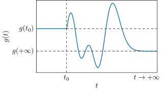
Figure 1: Sketch of a typical $g(t)$ [with arbitrary time units]: $g(t\to+\infty)$ is a constant and $g(t\leq t_{0})=g(t_{0})$. $t_{0}\to-\infty$ in the examples considered in Sec. IV, in these cases one further imposes that $g(t)$ tends to a constant value $g(-\infty)$ as $t\to-\infty$, with $\dot{g}(-\infty)=0$. In all the cases we consider $g(t)\geq 0$ for all times.

The key observation is that, under the above assumptions, the TDHO equation (51) has the same formal structure as the Schrödinger equation for a particle moving with zero energy in a static external potential $V_{\mathrm{ext}}<0$. The analogy relies on identifying, for the equivalent scattering problem, the physical time $t$ with an effective position $x_{\mathrm{eff}}=t$ such that $V_{\mathrm{ext}}(x_{\mathrm{eff}})=-\omega_{k}^{2}(t)$. Here $\omega_{k}(t)$ is given by Eq. (14), with $g(t)$ behaving as illustrated in Fig. 1. Thus, we are effectively studying a 1D quantum scattering problem along the time axis.

It is convenient to write the solution of Eq. (51) in the form

$$\gamma_{k}(t,t_{0})=e^{-i\omega_{k}(t_{0})(t-t_{0})}f_{k}(t,t_{0})\,,$$ (72)

where $f_{k}(t,t_{0})=1$ for $t\leq t_{0}$. Inserting the ansatz (72) into Eq. (51) one finds that $f_{k}$ obeys the second-order differential equation

$$\ddot{f}_{k}-2i\omega_{k}(t_{0})\dot{f}_{k}+[\omega_{k}^{2}(t)-\omega_{k}^{2}(t_{0})]f_{k}=0\,.$$ (73)

At large times the Bogoliubov frequency (14) approaches a constant value $\omega_{k}(+\infty)$. Consequently, the asymptotic expression of the solution of Eq. (51) takes the oscillating behavior

$$\begin{split}\gamma_{k}(t,t_{0})\underset{t\to+\infty}{=}&{}e^{i\omega_{k}(t_{0})t_{0}}\sqrt{\frac{\omega_{k}(t_{0})}{\omega_{k}(+\infty)}}\\ &{}\times\left[\tau^{\leftarrow}_{k}(t_{0})\,e^{-i\omega_{k}(+\infty)t}+\tau^{\rightarrow}_{k}(t_{0})\,e^{i\omega_{k}(+\infty)t}\right]\,.\end{split}$$ (74)

Here $\tau^{\leftarrow}_{k}(t_{0})$ and $\tau^{\rightarrow}_{k}(t_{0})$ play the role, in the equivalent 1D scattering problem, of the onward and backward transfer coefficient, respectively (see, e.g., Ref. LanLif03 ). The relation between these coefficients can be derived from Eq. (53), which is the analogous of the current conservation. Because of the particular choice of the prefactor in Eq. (74), at $t\to+\infty$ Eq. (53) takes the simple and intuitive form

$$|\tau^{\leftarrow}_{k}(t_{0})|^{2}-|\tau^{\rightarrow}_{k}(t_{0})|^{2}=1\,.$$ (75)

The transfer coefficients generally depend on the specific functional form of $g(t)$ and on the initial time $t_{0}$. In Appendix A we show how, starting from the knowledge of $\gamma_{k}(t,t_{0})$, $\tau^{\leftarrow}_{k}(t_{0})$, and $\tau^{\rightarrow}_{k}(t_{0})$ for a given $t_{0}$, it is possible to calculate the same quantities for any other initial time $t_{0}^{\prime}>t_{0}$.

The asymptotic behavior of the time-propagated weights (48) is easily deduced from the one of $\gamma_{k}$ of Eq. (74):

$$\begin{split}U_{k}(t,t_{0})\underset{t\to+\infty}{=}{}&{}e^{i\omega_{k}(t_{0})t_{0}}\Big{[}u_{k}(+\infty)\tau^{\leftarrow}_{k}(t_{0})e^{-i\omega_{k}(+\infty)t}\\ &{}\phantom{e^{i\omega_{k}(t_{0})t_{0}}\Big{[}}+v_{k}(+\infty)\tau^{\rightarrow}_{k}(t_{0})e^{i\omega_{k}(+\infty)t}\Big{]}\,,\end{split}$$ (76a)

$$\begin{split}V_{k}(t,t_{0})\underset{t\to+\infty}{=}{}&{}e^{i\omega_{k}(t_{0})t_{0}}\Big{[}v_{k}(+\infty)\tau^{\leftarrow}_{k}(t_{0})e^{-i\omega_{k}(+\infty)t}\\ &{}\phantom{e^{i\omega_{k}(t_{0})t_{0}}\Big{[}}+u_{k}(+\infty)\tau^{\rightarrow}_{k}(t_{0})e^{i\omega_{k}(+\infty)t}\Big{]}\,.\end{split}$$ (76b)

In turn, these expressions enable one to directly compute the asymptotic value of any observable.

Let us consider a system initially in its ground state at zero temperature. In this case the momentum distribution is [from Eq. (28)]

$$\begin{split}n_{\mathbf{k}}(t)\underset{t\to+\infty}{=}{}&{}\Big{|}v_{k}(+\infty)\tau^{\leftarrow}_{k}(t_{0})e^{-i\omega_{k}(+\infty)t}\\ {}&{}\phantom{\Big{|}}+u_{k}(+\infty)\tau^{\rightarrow}_{k}(t_{0})e^{i\omega_{k}(+\infty)t}\Big{|}^{2}\,,\end{split}$$ (77)

the anti-diagonal part of the four-point correlation function [from Eq. (33)] reads as

$$\begin{split}n^{(2)}_{\mathbf{k},-\mathbf{k}}(t)\underset{t\to+\infty}{=}&{}\Big{|}u_{k}(+\infty)\tau^{\leftarrow}_{k}(t_{0})e^{-i\omega_{k}(+\infty)t}\\ &\phantom{{}\Big{|}}+v_{k}(+\infty)\tau^{\rightarrow}_{k}(t_{0})e^{i\omega_{k}(+\infty)t}\Big{|}^{2}\\ &{}\times\Big{|}v_{k}(+\infty)\tau^{\leftarrow}_{k}(t_{0})e^{-i\omega_{k}(+\infty)t}\\ &\phantom{{}\times\Big{|}}+u_{k}(+\infty)\tau^{\rightarrow}_{k}(t_{0})e^{i\omega_{k}(+\infty)t}\Big{|}^{2}\,,\end{split}$$ (78)

and the structure factor (38) is given by

$$\begin{split}S(\mathbf{k},t)\underset{t\to+\infty}{=}\frac{\Omega_{k}}{\omega_{k}(+\infty)}{}&{}\Big{|}\tau^{\leftarrow}_{k}(t_{0})e^{-i\omega_{k}(+\infty)t}\\ {}&{}\phantom{\Big{|}}+\tau^{\rightarrow}_{k}(t_{0})e^{i\omega_{k}(+\infty)t}\Big{|}^{2}\,.\end{split}$$ (79)

It is worth pointing out that, in general, $n_{\mathbf{k}}(t)$, $n^{(2)}_{\mathbf{k},-\mathbf{k}}(t)$, and $S(\mathbf{k},t)$ keep oscillating in time even at large $t$. As first discussed in Ref. Hun13 and re-analyzed below, these oscillations are analogous to the cosmological Sakharov oscillations Sak65 ; Gri12b , which originate in acoustic vibrations in the primordial plasma of the early universe before the epoch of recombination. Despite this time dependence, in 3D it is possible to prove that the condensate depletion is time independent at large $t$ (see Appendix B) and can be expressed as

$$\begin{split}\Delta N(t)\underset{t\to+\infty}{=}V\int\frac{d^{3}k}{(2\pi)^{3}}\Big{[}{}&{}|v_{k}(+\infty)\tau^{\leftarrow}_{k}(t_{0})|^{2}\\ &{}+|u_{k}(+\infty)\tau^{\rightarrow}_{k}(t_{0})|^{2}\Big{]}\,.\end{split}$$ (80)

Concerning the Sakharov oscillations, the situation is particularly simple when $g(+\infty)=0$. In this case one has $\omega_{k}(+\infty)=\Omega_{k}$, $u_{k}(+\infty)=1$, and $v_{k}(+\infty)=0$. Then, $n_{\mathbf{k}}$ and $n^{(2)}_{\mathbf{k},-\mathbf{k}}$ become time independent at large time, as clearly seen from Eqs. (77) and (78):

$$n_{\mathbf{k}}(t) {}\underset{t\to+\infty}{=}|\tau^{\rightarrow}_{k}(t_{0})|^{2}\,,$$ (81a)

$$n^{(2)}_{\mathbf{k},-\mathbf{k}}(t) {}\underset{t\to+\infty}{=}|\tau^{\leftarrow}_{k}(t_{0})|^{2}|\tau^{\rightarrow}_{k}(t_{0})|^{2}\,.$$ (81b)

However, except for the exceptional cases discussed below, $S(\mathbf{k},t)$ remains a time-dependent function, oscillating at period $\pi/\omega_{k}(+\infty)$. This can be understood as resulting from the creation of pairs of excitations during the epoch of time-dependent $g(t)$. Because the system is homogeneous, momentum conservation imposes that the excitations are created with opposite momenta $\pm\mathbf{k}$. In our model these pairs, once created, survive when $g(t)$ reaches its final zero value, and subsequently interfere constructively each half of their common period.

A rather interesting situation occurs when one has total transmission across the potential barrier for some $k$. This corresponds to the condition $\tau^{\rightarrow}_{k}(t_{0})=0$ or, equivalently, $|\tau^{\leftarrow}_{k}(t_{0})|=1$. For these modes the asymptotic values of the time-propagated weights (76) coincide, up to a phase factor, with the corresponding instantaneous weights (13) at $t\to+\infty$. As a consequence, for this specific values of $k$, all the $k$-dependent observables [including the momentum distribution (77), the four-point correlation function (78), and even the structure factor (79)] are stationary even if $g(+\infty)\neq 0$. Moreover, their values coincide with those obtained for a BEC with time-independent coupling equal to $g(+\infty)$. This observation is also related to the discussion of Sec. III.3 about adiabatic evolution. In fact, by noting that $\int_{t_{0}}^{t}dt^{\prime}\,\omega_{k}(t^{\prime})\sim\omega_{k}(+\infty)t+\mathrm{const}.$ for $t\to+\infty$, one finds that the large-$t$ behavior of Eq. (66) is of the kind (76) with $|\tau^{\leftarrow}_{k}(t_{0})|=1$ and $\tau^{\rightarrow}_{k}(t_{0})=0$. This means that adiabaticity implies total transmission across the potential barrier.

Up to now we have always assumed the initial time $t_{0}$ to be finite. It actually makes sense to consider cases where $t_{0}\to-\infty$, as we do in Sec. IV. The only additional requirements are that $g(t)$ tends to a constant value $g(-\infty)$ at large negative times and $\dot{g}(-\infty)=0$. Notice that the global phase factor $\exp[i\omega_{k}(t_{0})t_{0}]$, first introduced in Eq. (72) and subsequently entering the time-propagated weights (76), is ill defined if $t_{0}\to-\infty$. However, this phase factor does not represent a problem because it systematically cancels when computing any observable [for example, it no longer appears in Eqs. (77), (78), and (79)].

Finally, it is worth stressing that all the large-time expressions of the present section have been derived within the framework of Bogoliubov theory. The latter neglects the interaction between quasiparticles, which is expected to lead to relaxation in our quantum many-body system at times $t\gg\hbar/[g(+\infty)\rho]$ (see Ref. VanR18 ). The study of such effects goes beyond the scope of this work, within which the $t\to+\infty$ limit means that $t$ is much larger than the typical scale of time variation of $g(t)$, while remaining smaller than the thermalization time.

IV Exactly solvable models

In this section we discuss in detail three examples where the TDHO equation (51) can be solved analytically. These are the steplike (Sec. IV.1), the Woods-Saxon (Sec. IV.2), and the modified Pöschl-Teller coupling (Sec. IV.3). Other solvable models may be considered, for instance the linear piecewise $g(t)$ studied in Refs. Ber14 ; Sch18 .

IV.1 Steplike coupling

The simplest case in which one can calculate everything analytically is when the coupling constant has a steplike behavior. Let us take

$$g(t)=\begin{cases}g_{0}&\mbox{if}\;\;t<0\,,\\ g_{1}&\mbox{if}\;\;t>0\,.\end{cases}$$ (82)

We indicate by $\omega_{k,0}$ and $\omega_{k,1}$ the Bogoliubov frequency (14) before and after the jump, respectively; the corresponding instantaneous weights (13) are denoted by $u_{k,0}$, $v_{k,0}$ and $u_{k,1}$, $v_{k,1}$.

The problem is trivial for $t_{0}>0$, hence, in this section we take $t_{0}<0$. For negative $t$, before the jump, the solution of Eq. (51) with initial value (52) is simply $\gamma_{k}(t,t_{0})=\exp[-i\omega_{k,0}(t-t_{0})]$. After the jump $\gamma_{k}$ must be a linear combination of the two oscillating exponentials $\exp(\pm i\omega_{k,1}t)$. By requiring the continuity of $\gamma_{k}$ and its first-order derivative one finds, for $t>0$,

$$\begin{split}\gamma_{k}(t,t_{0})=e^{i\omega_{k,0}t_{0}}\sqrt{\frac{\omega_{k,0}}{\omega_{k,1}}}\left(\tau^{\leftarrow}_{k}\,e^{-i\omega_{k,1}t}+\tau^{\rightarrow}_{k}\,e^{i\omega_{k,1}t}\right)\,.\end{split}$$ (83)

Here, the transfer coefficients are independent of $t_{0}$ and read as

$$\begin{split}\tau^{\leftarrow}_{k}&{}=\frac{1}{2}\left(\sqrt{\frac{\omega_{k,1}}{\omega_{k,0}}}+\sqrt{\frac{\omega_{k,0}}{\omega_{k,1}}}\right)\,,\\ \tau^{\rightarrow}_{k}&{}=\frac{1}{2}\left(\sqrt{\frac{\omega_{k,1}}{\omega_{k,0}}}-\sqrt{\frac{\omega_{k,0}}{\omega_{k,1}}}\right)\,.\end{split}$$ (84)

The time-propagated weights (48) and all the observables can be easily computed from the above formulas. In particular, before the jump the observables are stationary. Instead, for a system initially in its ground state at zero temperature, after the jump the momentum distribution, the anti-diagonal four-point correlation function, and the structure factor are obtained by inserting Eqs. (84) into (77), (78), and (79) (notice that all the asymptotic formulas given in Sec. III.4 exactly hold at any $t>0$ for a steplike coupling). This yields

$$\begin{split}n_{\mathbf{k}}(t)=\left|v_{k,0}\right|^{2}+\frac{g_{1}(g_{1}-g_{0})\rho^{2}\sin^{2}\omega_{k,1}t}{(\hbar\Omega_{k}+2g_{1}\rho)\sqrt{\hbar\Omega_{k}(\hbar\Omega_{k}+2g_{0}\rho)}}\,,\end{split}$$ (85)

$$n^{(2)}_{\mathbf{k},-\mathbf{k}}(t)=n_{\mathbf{k}}(t)[n_{\mathbf{k}}(t)+1]\,,$$ (86)

and

$$S(\mathbf{k},t)=\frac{\Omega_{k}}{\omega_{k,0}}\left(1+\frac{\omega_{k,0}^{2}-\omega_{k,1}^{2}}{\omega_{k,1}^{2}}\sin^{2}\omega_{k,1}t\right)\,.$$ (87)

Concerning the quantum depletion, after integration the first term on the right-hand side of Eq. (85) returns the depletion (41) of the condensate before the jump. The integral of the second term can be easily computed in the large-$t$ limit. To this purpose one needs to replace $\sin^{2}\omega_{k,1}t$ with $\frac{1}{2}$ (see Appendix B) and to change the integration variable from $k$ to $\tilde{k}=\sqrt{(\hbar\Omega_{k}+2g_{0}\rho)/(2|g_{1}-g_{0}|\rho)}$. The final result is

$$\Delta N(t)\underset{t\to+\infty}{=}\frac{V}{3\pi^{2}\xi_{0}^{3}}+\frac{V}{2\pi^{2}\xi_{1}^{3}}\,\Delta\tilde{N}\,.$$ (88)

Here $\xi_{(0,1)}=\hbar/\sqrt{mg_{(0,1)}\rho}$ are the initial and final healing lengths, and

$$\Delta\tilde{N}=\begin{cases}+\frac{\sqrt{g_{1}^{2}-g_{0}^{2}}}{g_{1}}\operatorname{arccot}\sqrt{\frac{g_{0}}{g_{1}-g_{0}}}&\mbox{if}\;\;g_{1}>g_{0}\,,\\ -\frac{\sqrt{g_{0}^{2}-g_{1}^{2}}}{g_{1}}\operatorname{arccoth}\sqrt{\frac{g_{0}}{g_{0}-g_{1}}}&\mbox{if}\;\;g_{1}<g_{0}\,.\end{cases}$$ (89)

Two limiting cases deserve special attention. If $g_{1}=0$ one has $\omega_{k,1}=\Omega_{k}$, $u_{k,1}=1$, $v_{k,1}=0$, $\tau^{\leftarrow}_{k}=u_{k,0}$, and $\tau^{\rightarrow}_{k}=v_{k,0}$. Inserting this relations into Eqs. (76) one finds that the time-propagated weights at $t>0$ coincide, up to an oscillating phase, with the instantaneous ones before the jump. This implies that the momentum distribution remains frozen to its initial value of Eq. (32) even at $t>0$,

$$n_{\mathbf{k}}(t)=\left|v_{k,0}\right|^{2}\,,$$ (90)

as one can check directly from Eq. (85). The same behavior is also exhibited by the four-point correlation function and the quantum depletion. It is worth pointing out that this prediction is consistent with the results of the recent experiment Lop17 . In this reference the authors measured the momentum distribution of a uniform BEC after turning off the interaction and the trapping potential, showing that it retains the same value as the prequench one.

If, instead, $g_{0}=0$, i.e., $\omega_{k,0}=\Omega_{k}$, the transfer coefficients (84) simplify to $\tau^{\leftarrow}_{k}=u_{k,1}$ and $\tau^{\rightarrow}_{k}=-v_{k,1}$. The momentum distribution at $t>0$ then becomes

$$n_{\mathbf{k}}(t)=\left|2u_{k,1}v_{k,1}\right|^{2}\sin^{2}(\omega_{k,1}t)\,.$$ (91)

and the asymptotic value of the quantum depletion is $\Delta N(t\to+\infty)=V/(4\pi\xi_{1}^{3})$. This is larger by a factor $3\pi/4\simeq 2.36$ than the depletion of a static condensate with coupling $g_{1}$.

IV.2 Woods-Saxon coupling

Let us now consider a time-dependent coupling constant of the kind

$$g(t)=g_{1}+\frac{g_{0}-g_{1}}{1+e^{t/\tau}}\,,$$ (92)

which has the same analytic form as the Woods-Saxon potential commonly employed in nuclear physics. This coupling has been studied numerically in Ref. Rob17a ; the corresponding scattering problem is known to be exactly solvable, cf. (LanLif03, , §25, Problem 3). The Woods-Saxon coupling varies smoothly and monotonically from $g(-\infty)=g_{0}$ to $g(+\infty)=g_{1}$ (see Fig. 2), the time scale for the change being fixed by $\tau$. In the $\tau\to 0$ limit Eq. (92) tends to the steplike coupling (82), and all the formulas that we are going to deduce in the present section reduce to the corresponding ones of Sec. IV.1. It is worth pointing out that, although here we only address the $t_{0}\to-\infty$ case, this choice is not too restrictive. Indeed, once the solution for this special case is known, one can use the procedure of Appendix A to extend the results to arbitrary $t_{0}$.

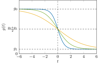
Figure 2: Woods-Saxon coupling (92) as a function of time. Here $g_{1}/g_{0}=0.1$ and $\tau=0.5$ [blue (dark gray) curve], $1.0$ [green (intermediate gray) curve], $2.0$ [yellow (light gray) curve]. Times are in units of $\hbar/(g_{0}\rho)$. Although the drawing illustrates the case $g_{1}<g_{0}$, the results of the present section hold true also when $g_{1}>g_{0}$.

Equation (73) for the Woods-Saxon coupling with $t_{0}\to-\infty$ becomes

$$\ddot{f}_{k}-2i\omega_{k,0}\dot{f}_{k}+(\omega_{k,1}^{2}-\omega_{k,0}^{2})\frac{e^{t/\tau}}{1+e^{t/\tau}}f_{k}=0\,,$$ (93)

where we have adopted the same abbreviated notation $\omega_{k,0}=\omega_{k}(-\infty)$ and $\omega_{k,1}=\omega_{k}(+\infty)$ as in Sec. IV.1. After changing variable from $t$ to $\zeta=-\exp(t/\tau)$ we obtain

$$\zeta(1-\zeta)\frac{d^{2}f_{k}}{d\zeta^{2}}+[c_{k}-(1+a_{k}+b_{k})\zeta]\frac{df_{k}}{d\zeta}-a_{k}b_{k}f_{k}=0\,,$$ (94)

where we have defined the parameters

$$\begin{split}a_{k}&{}=i(\omega_{k,1}-\omega_{k,0})\tau\,,\\ b_{k}&{}=-i(\omega_{k,1}+\omega_{k,0})\tau\,,\\ c_{k}&{}=1-2i\omega_{k,0}\tau\,.\end{split}$$ (95)

Equation (94) corresponds to the well-known hypergeometric differential equation Abr65 . There are two independent exact solutions available for this equation. The first one is $f_{k}(\zeta)={}_{2}F_{1}(a_{k},b_{k},c_{k};\zeta)$, where ${}_{2}F_{1}$ denotes the hypergeometric function. From Eq. (72) one deduces the corresponding solution of the TDHO equation (51),

$$\gamma_{k}(t,t_{0}\to-\infty)=e^{-i\omega_{k,0}(t-t_{0})}{}_{2}F_{1}(a_{k},b_{k},c_{k};-e^{t/\tau})\,.$$ (96)

This expression fulfills the initial conditions (52), as can be easily checked by recalling that ${}_{2}F_{1}(a_{k},b_{k},c_{k};0)=1$. Notice that the calculation of the derivative of $\gamma_{k}$ requires the use of the relation $\frac{d}{d\zeta}\,{}_{2}F_{1}(a_{k},b_{k},c_{k};\zeta)=\frac{a_{k}b_{k}}{c_{k}}\,{}_{2}F_{1}(a_{k}+1,b_{k}+1,c_{k}+1;\zeta)$.

For completeness, we mention that the second independent solution of Eq. (94) is $f_{k}(\zeta)=\zeta^{1-c_{k}}{}_{2}F_{1}(1+a_{k}-c_{k},1+b_{k}-c_{k},2-c_{k};\zeta)$. Inserting this expression into Eq. (72) one gets (up to an irrelevant constant factor) the complex conjugate of Eq. (96). To verify this, one can first note that from Eqs. (95) the three relations $1+a_{k}-c_{k}=b_{k}^{*}$, $1+b_{k}-c_{k}=a_{k}^{*}$, and $2-c_{k}=c_{k}^{*}$ follow. The above statement is then readily proved using the identity ${}_{2}F_{1}(b_{k}^{*},a_{k}^{*},c_{k}^{*};\zeta)=[{}_{2}F_{1}(a_{k},b_{k},c_{k};\zeta)]^{*}$, holding for real $\zeta$. However this solution is not acceptable because it does not fulfill the initial conditions (52).

Strictly speaking, the hypergeometric function ${}_{2}F_{1}(a_{k},b_{k},c_{k};\zeta)$ is defined only for $\left|\zeta\right|<1$. This means that Eq. (96) is valid only for negative $t$. However, it can be extended by analytic continuation to $t\geq 0$, as discussed in Appendix C. In particular, employing the transformation (148a) one can see that the large-$t$ behavior is of the kind (74), with

$$\begin{split}\tau^{\leftarrow}_{k}(t_{0}\to-\infty)&{}=\sqrt{\frac{b_{k}-a_{k}}{b_{k}+a_{k}}}\frac{\Gamma(c_{k})\Gamma(b_{k}-a_{k})}{\Gamma(b_{k})\Gamma(c_{k}-a_{k})}\,,\\ \tau^{\rightarrow}_{k}(t_{0}\to-\infty)&{}=\sqrt{\frac{b_{k}-a_{k}}{b_{k}+a_{k}}}\frac{\Gamma(c_{k})\Gamma(a_{k}-b_{k})}{\Gamma(a_{k})\Gamma(c_{k}-b_{k})}\,,\end{split}$$ (97)

where $\Gamma$ is the gamma function.

Now we have everything we need to compute exactly all the observables of interest. We start by looking at the zero-temperature momentum distribution at long evolution times. In Fig. 3 we plot the typical behavior of this quantity at two different (and large) values of $t$. It can be clearly seen that it is non-monotonous and it varies over time. We have checked that the results obtained from the exact expression (31) are in excellent agreement with the asymptotic estimate (77) in this large-$t$ regime.

Figure 4 shows the quantum depletion (40) as a function of time for two different choices of the final coupling strength $g_{1}$. We consider several values of the characteristic time $\tau$, including $\tau=0$, which corresponds to the steplike coupling investigated in Sec. IV.1. The exact results (solid lines) are compared with the adiabatic prediction (71) (dashed lines). Notice that the discrepancy between the two is significant when $\tau$ is small, and particularly for $\tau=0$; however, the agreement becomes extremely good for the largest values of $\tau$ that we consider.

The existence of a crossover between nonadiabatic and adiabatic behavior of the quantum depletion as $\tau$ increases becomes more evident by looking at Fig. 5. Here we plot the asymptotic value (80) of the depletion as a function of $\tau$. One can see that for $\tau\to 0$ it approaches the steplike result (88), while as $\tau\to+\infty$ it goes asymptotically to the adiabatic value $V/(3\pi^{2}\xi_{1}^{3})$.

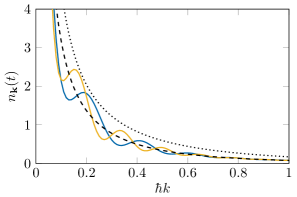
Figure 3: Asymptotic value of the momentum distribution for the Woods-Saxon coupling as a function of momentum. Here $g_{1}/g_{0}=0.5$, $\tau=1.0$, $t_{0}\to-\infty$, and $t=20.0$ [blue (dark gray) solid curve], $25.0$ [yellow (light gray) solid curve]. At each $\mathbf{k}$, $n_{\mathbf{k}}(t)$ oscillates around the value $|v_{k}(+\infty)\tau^{\leftarrow}_{k}(t_{0})|^{2}+|u_{k}(+\infty)\tau^{\rightarrow}_{k}(t_{0})|^{2}$, that is indicated by the black dashed curve. For comparison, we also plot the initial momentum distribution (32) (black dotted curve). Times are in units of $\hbar/(g_{0}\rho)$. Momentum is in units of $\sqrt{mg_{0}\rho}$.

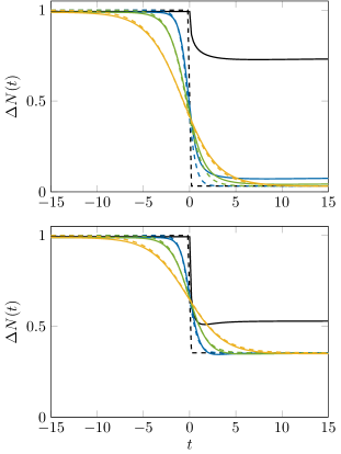
Figure 4: Quantum depletion for the Woods-Saxon coupling as a function of time for $g_{1}/g_{0}=0.1$ (top) and $g_{1}/g_{0}=0.5$ (bottom). Here $t_{0}\to-\infty$ and $\tau=0.0$ (black curves), $0.5$ [blue (dark gray) curves], $1.0$ [green (intermediate gray) curves], $2.0$ [yellow (light gray) curves]. The solid and dashed lines show the exact results and the adiabatic prediction (71), respectively. Times are in units of $\hbar/(g_{0}\rho)$. The depletion is in units of $V/(3\pi^{2}\xi_{0}^{3})$.

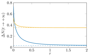
Figure 5: Asymptotic value of the quantum depletion for the Woods-Saxon coupling as a function of characteristic time. Here $t_{0}\to-\infty$ and $g_{1}/g_{0}=0.1$ [blue (dark gray) solid curve], $0.5$ [yellow (light gray) solid curve]. The dashed lines indicate the adiabatic prediction $V/(3\pi^{2}\xi_{1}^{3})$ corresponding to the two above choices of $g_{1}/g_{0}$. Times are in units of $\hbar/(g_{0}\rho)$. The depletion is in units of $V/(3\pi^{2}\xi_{0}^{3})=\Delta N(t\to-\infty)$.

Let us now consider the simplest case $g_{1}=0$ and a system initially in its ground state at $T=0$. According to Eq. (81a), the stationary value of the $T=0$ momentum distribution at large $t$ coincides with the square modulus of the coefficient $\tau^{\rightarrow}_{k}(t_{0}\to-\infty)$ given in Eq. (97). The analytic formula for this quantity can be significantly simplified using the identities $[\Gamma(z)]^{*}=\Gamma(z^{*})$, $\Gamma(1+z)=z\Gamma(z)$, $\Gamma(z)\Gamma(1-z)=\pi/\sin(\pi z)$ (reflection formula), and $\sin(iz)=i\sinh z$. Taking the expressions (95) of the parameters $a_{k}$, $b_{k}$, and $c_{k}$ into account and setting $\omega_{k,1}=\Omega_{k}$, one eventually obtains

$$n_{\mathbf{k}}(t)\underset{t\to+\infty}{=}\frac{\sinh^{2}[\pi(\Omega_{k}-\omega_{k,0})\tau]}{\sinh(2\pi\Omega_{k}\tau)\sinh(2\pi\omega_{k,0}\tau)}\,.$$ (98)

Notice that in the $k\to 0$ regime the behavior of the asymptotic momentum distribution, $n_{\mathbf{k}}(t\to+\infty)\sim mc_{0}/2\hbar k$ [here $c_{0}=c(-\infty)$], is the same as at the initial time $t_{0}\to-\infty$. This is in full agreement with the general findings of Sec. III.2. In the opposite limit $k\to+\infty$ one has instead $n_{\mathbf{k}}(t\to+\infty)\sim 4\sinh^{2}(\pi mc_{0}^{2}\tau/\hbar)\exp[-2\pi(\hbar\tau/m)k^{2}]$.

The anti-diagonal four-point correlation function for $g_{1}=0$ can be calculated starting from Eq. (81b). Proceeding as we did for the momentum distribution, we end up with

$$\begin{split}n^{(2)}_{\mathbf{k},-\mathbf{k}}(t)\underset{t\to+\infty}{=}{}&{}\\ {}&{}\left\{\frac{\sinh[\pi(\Omega_{k}-\omega_{k,0})\tau]\sinh[\pi(\Omega_{k}+\omega_{k,0})\tau]}{\sinh(2\pi\Omega_{k}\tau)\sinh(2\pi\omega_{k,0}\tau)}\right\}^{2}\,.\end{split}$$ (99)

IV.3 Modified Pöschl-Teller coupling

The modified Pöschl-Teller coupling is defined as

$$g(t)=g_{1}+\frac{g_{0}-g_{1}}{\cosh^{2}(t/\tau)}\,.$$ (100)

This coupling changes monotonically starting from the value $g_{1}$ at $t\to-\infty$, reaches the value $g_{0}$ at $t=0$, and then goes back to $g_{1}$ for $t\to+\infty$. $g(t)$ is an even function of time, and attains a minimum (maximum) at $t=0$ when $g_{0}<g_{1}$ ($g_{0}>g_{1}$ as illustrated in Fig. 6). As for the Woods-Saxon coupling, a finite scale $\tau$ quantifies how rapidly the coupling changes over time.

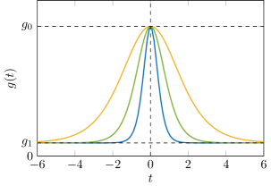
Figure 6: Modified Pöschl-Teller coupling (100) as a function of time. Here $g_{1}/g_{0}=0.1$ and $\tau=0.5$ [blue (dark gray) curve], $1.0$ [green (intermediate gray) curve], $2.0$ [yellow (light gray) curve]. Times are in units of $\hbar/(g_{0}\rho)$.

Equation (73) with the modified Pöschl-Teller coupling and $t_{0}\to-\infty$ reads

$$\ddot{f}_{k}-2i\omega_{k,1}\dot{f}_{k}+\frac{\omega_{k,0}^{2}-\omega_{k,1}^{2}}{\cosh^{2}(t/\tau)}f_{k}=0\,.$$ (101)

Notice that here and in the rest of the present section we are using the notation $\omega_{k,0}=\omega_{k}(0)$ and $\omega_{k,1}=\omega_{k}(\pm\infty)$. We deal with Eq. (101) in a way similar to the one illustrated in (LanLif03, , §23, Problem 5 and §25, Problem 4). Changing the variable to $\zeta=[1+\tanh(t/\tau)]/2$ it becomes

$$\zeta(1-\zeta)\frac{d^{2}f_{k}}{d\zeta^{2}}+(c_{k}-2\zeta)\frac{df_{k}}{d\zeta}+s_{k}(s_{k}+1)f_{k}=0\,.$$ (102)

Here we have introduced the two quantities

$$\begin{split}&s_{k}=\frac{1}{2}\left[\sqrt{4(\omega_{k,0}^{2}-\omega_{k,1}^{2})\tau^{2}+1}-1\right]\,,\\ &c_{k}=1-i\omega_{k,1}\tau\,.\end{split}$$ (103)

Notice that $s_{k}$ is always a real positive number if $g_{0}>g_{1}$. It is instead real and negative if $g_{1}>g_{0}$ and $4(\omega_{k,0}^{2}-\omega_{k,1}^{2})\tau^{2}+1\geq 0$, that is, $k\leq\sqrt{m/[4(g_{1}-g_{0})\rho\tau^{2}]}$. In all the other cases $s_{k}$ becomes complex.

Equation (102) has the same form as the hypergeometric equation (94) with $a_{k}=-s_{k}$ and $b_{k}=s_{k}+1$. Consequently, its solutions are expressed in terms of hypergeometric functions. The first independent solution that we consider is $f_{k}(\zeta)={}_{2}F_{1}(-s_{k},s_{k}+1,c_{k};\zeta)$. By plugging it into Eq. (72) one gets

$$\begin{split}\gamma_{k}(t,t_{0}\to-\infty)={}&{}e^{-i\omega_{k,1}(t-t_{0})}\\ &{}\times{}_{2}F_{1}\left(-s_{k},s_{k}+1,c_{k};\textstyle\frac{e^{2t/\tau}}{e^{2t/\tau}+1}\right)\,.\end{split}$$ (104)

This function satisfies both the TDHO equation (51) and the initial conditions (52). Thus, it will be used in all the calculations of the remaining part of the present section.

The second independent solution of Eq. (102) is $f_{k}(\zeta)=\zeta^{1-c_{k}}{}_{2}F_{1}(1-s_{k}-c_{k},2+s_{k}-c_{k},2-c_{k};\zeta)$. Here, the same thing happens as for the Woods-Saxon coupling: this second solution is not acceptable because it does not fulfill the initial conditions (52).

The transfer coefficients for the modified Pöschl-Teller coupling can be obtained by applying the transformation (148b) to Eq. (104) and taking the large-$t$ limit. The result is

$$\begin{split}\tau^{\leftarrow}_{k}(t_{0}\to-\infty)&{}=\frac{\Gamma(c_{k})\Gamma(c_{k}-1)}{\Gamma(c_{k}+s_{k})\Gamma(c_{k}-s_{k}-1)}\,,\\ \tau^{\rightarrow}_{k}(t_{0}\to-\infty)&{}=\frac{\Gamma(c_{k})\Gamma(1-c_{k})}{\Gamma(-s_{k})\Gamma(s_{k}+1)}\,.\end{split}$$ (105)

An interesting consequence of Eq. (105) is that the modified Pöschl-Teller coupling supports total transmission if $g_{0}>g_{1}$. Indeed, $\Gamma(-s_{k})$ diverges if $s_{k}$ is a non-negative integer, which entails the vanishing of $\tau^{\rightarrow}_{k}(t_{0}\to-\infty)$. This happens whenever

$$k=\sqrt{\frac{p(p+1)m}{(g_{0}-g_{1})\rho\tau^{2}}}\,,\quad p\in\mathbb{N}\,.$$ (106)

As discussed at the end of Sec. III.4, when $k$ fulfills the resonance condition (106) the $k$-dependent observables are stationary at large times; their values coincide with those of a BEC with constant coupling $g_{1}$. Additionally, if $g_{1}=0$, the momentum distribution and the four-point correlation function have a non-monotonous behavior even if they are stationary at all $k$’s, and they vanish at the resonant momenta (106) [see Eqs. (107) and (108) below]. All these considerations hold for the $t_{0}\to-\infty$ case, but the scenario can partly persist if one switches to finite $t_{0}$ (see Appendix A). As shown in Fig. 7, resonant and quasi-resonant situations are possible if $t_{0}$ is not too close to $0$ or positive.

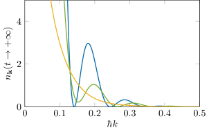
Figure 7: Asymptotic value of the momentum distribution for the modified Pöschl-Teller coupling as a function of momentum. Here, $g_{1}=0$, $\tau=10.0$, $t_{0}=-\infty$ [blue (dark gray) curve], $-20.0$ [green (intermediate gray) curve], $0.0$ [yellow (light gray) curve]. Times are in units of $\hbar/(g_{0}\rho)$. Momentum is in units of $\sqrt{mg_{0}\rho}$.

The behavior of the quantum depletion (40) as a function of time is shown in Fig. 8 for several values of $\tau$ and $g_{1}/g_{0}$ (here, and in all the rest of this section, we consider a system initially in its ground state at $T=0$). As already seen in Sec. IV.2 for the Woods-Saxons coupling, the exact prediction gets closer and closer to the adiabatic one (71) as $\tau$ increases.

In Fig. 9 we plot the asymptotic depletion (80) as a function of $\tau$. The behavior of the curve follows from the property that the initial and final values of the coupling coincide. For small $\tau$, a large number of modes fall in the small-$k$ part of the momentum distribution that stays frozen. Consequently, the depletion remains approximately constant in time. At large $\tau$, instead, the majority of the modes are in the large-$k$ tail that behaves adiabatically. Thus, the depletion goes back to its initial value at the end of the time evolution. For these two reasons, the values of the depletion before and after time evolution can differ significantly from each other only for intermediate $\tau$.

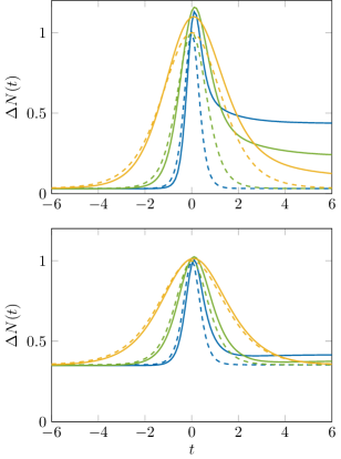
Figure 8: Quantum depletion for the modified Pöschl-Teller coupling as a function of time for $g_{1}/g_{0}=0.1$ (top) and $g_{1}/g_{0}=0.5$ (bottom). Here, $t_{0}\to-\infty$ and $\tau=0.5$ [blue (dark gray) curves], $1.0$ [green (intermediate gray) curves], $2.0$ [yellow (light gray) curves]. The solid and dashed lines show the exact results and the adiabatic prediction (71), respectively. Times are in units of $\hbar/(g_{0}\rho)$. The depletion is in units of $V/(3\pi^{2}\xi_{0}^{3})$.

Figure 9: Asymptotic value of the quantum depletion for the modified Pöschl-Teller coupling as a function of characteristic time. Here, $t_{0}\to-\infty$ and $g_{1}/g_{0}=0.1$ [blue (dark gray) solid curve], $0.5$ [yellow (light gray) solid curve]. The black dashed line indicates the adiabatic prediction $V/(3\pi^{2}\xi_{1}^{3})$. Times are in units of $\hbar/(g_{1}\rho)$. The depletion is in units of $V/(3\pi^{2}\xi_{1}^{3})=\Delta N(t\to-\infty)$.

Let us now go back briefly to the case $t_{0}=-\infty$ and $g_{1}=0$. According to Eq. (81a), the stationary value of the momentum distribution at zero temperature can be found by computing the square modulus of the coefficient $\tau^{\rightarrow}_{k}(t_{0}\to-\infty)$ given in Eq. (105) and setting $\omega_{k,1}=\Omega_{k}$. The calculation is very similar to the one that led us to Eq. (98). The result is

$$n_{\mathbf{k}}(t)\underset{t\to+\infty}{=}\frac{\cos^{2}\left[\frac{\pi}{2}\sqrt{4(\omega_{k,0}^{2}-\Omega_{k}^{2})\tau^{2}+1}\,\right]}{\sinh^{2}(\pi\Omega_{k}\tau)}\,.$$ (107)

At $k\to+\infty$, $n_{\mathbf{k}}(t\to+\infty)$ decreases exponentially to $0$, very roughly as $\exp[-\pi(\hbar\tau/m)k^{2}]$. Instead, at $k\to 0$ the momentum distribution tends to a finite value $n_{\mathbf{k}=0}(t\to+\infty)=(2g_{0}\rho\tau/\hbar)^{2}$. The latter could equally be obtained by calculating the integral (59b) and taking its square modulus. The anti-diagonal four-point correlation function at zero temperature can be deduced from Eq. (81b) and reads as

$$n^{(2)}_{\mathbf{k},-\mathbf{k}}(t)\underset{t\to+\infty}{=}n_{\mathbf{k}}(t)[n_{\mathbf{k}}(t)+1]\,.$$ (108)

V Quantum coherence in 3D and 1D

The degree of quantum coherence of the system is characterized by its one-body density matrix, defined in terms of the field operator $\hat{\Psi}(\mathbf{r},t)$ as Dal99 ; PitStr16

$$\rho^{(1)}(\mathbf{r},\mathbf{r}^{\prime},t)=\langle\hat{\Psi}^{\dagger}(\mathbf{r},t)\hat{\Psi}(\mathbf{r}^{\prime},t)\rangle\,.$$ (109)

In the weakly interacting regime considered in this work, $\rho^{(1)}$ can be computed in dimension $d=3$ within the standard Bogoliubov theory of linearized quantum fluctuations. In lower dimension, when $d=1$ or $2$, the large phase fluctuations of $\hat{\Psi}(\mathbf{r},t)$ drastically affect the phase coherence of the system and destroy Bose-Einstein condensation, the existence of which is at the heart of standard Bogoliubov theory. However, even in this case, generalized Bogoliubov theories Pop72 ; Pop83 ; Mor03 ; Lar13 may be employed for calculating $\rho^{(1)}$ in the limit of weak interactions and small density fluctuations. The correct treatment, valid in any dimension and for any separation $|\mathbf{r}-\mathbf{r}^{\prime}|$, yields for our nonequilibrium system Lar16 ; Lar18

$$\rho^{(1)}(\mathbf{r},\mathbf{r}^{\prime},t)=\rho\,\exp\!\bigg{[}{-}\frac{\Delta\rho(\mathbf{r},\mathbf{r},t)-\Delta\rho(\mathbf{r},\mathbf{r}^{\prime},t)}{\rho}\bigg{]}\,,$$ (110)

where $\Delta\rho(\mathbf{r},\mathbf{r}^{\prime},t)$ is expressed in terms of the quench-dependent Bogoliubov momentum distribution $n_{\mathbf{k}}(t)$ as

$$\Delta\rho(\mathbf{r},\mathbf{r}^{\prime},t)=\int\frac{d^{d}k}{(2\pi)^{d}}\,n_{\mathbf{k}}(t)\cos[\mathbf{k}\cdot(\mathbf{r}-\mathbf{r}^{\prime})]\,,$$ (111)

and we recall that $\rho=\rho^{(1)}(\mathbf{r},\mathbf{r},t)$ is the density of the gas, here homogeneous.

When $d=3$, the argument of the exponential in Eq. (110) is small and one may approximate the one-body density matrix by

$$\rho^{(1)}(\mathbf{r},\mathbf{r}^{\prime},t)\simeq\rho-\Delta\rho(\mathbf{r},\mathbf{r},t)+\Delta\rho(\mathbf{r},\mathbf{r}^{\prime},t)\,.$$ (112)

This expression easily compares with the Bogoliubov prediction for $\rho^{(1)}$ Dal99 ; PitStr16 , only valid in 3D. In particular, $\rho-\Delta\rho(\mathbf{r},\mathbf{r},t)=\rho_{0}(t)$ is nothing but the density of the condensate, obtained by subtracting to the mean density $\rho$ of the gas the quantum depletion

$$\Delta\rho(\mathbf{r},\mathbf{r},t)=\int\frac{d^{3}k}{(2\pi)^{3}}\,n_{\mathbf{k}}(t)=\frac{\Delta N(t)}{V}$$ (113)

[see Eq. (40)]. In this case, off-diagonal long-range order is achieved since the remaining term in Eq. (112), $\Delta\rho(\mathbf{r},\mathbf{r}^{\prime},t)$, vanishes for distant $\mathbf{r}$ and $\mathbf{r}^{\prime}$, and in this case $\rho^{(1)}$ tends to a finite value equal to the density of the condensate:

$$\rho^{(1)}(\mathbf{r},\mathbf{r}^{\prime},t)\xrightarrow[|\mathbf{r}-\mathbf{r}^{\prime}|\to+\infty]{}\rho_{0}(t)\,.$$ (114)

Note that the long-time density $\rho_{0}(t\to+\infty)$ of the condensate is well defined since, as shown in Sec. III.4, $\Delta N(t)$ tends to a constant as $t\to+\infty$ [see Eq. (80)].

In lower dimension ($d=1$ or $2$), the large phase fluctuations of the field operator rule out Bose-Einstein condensation Mer66 ; Hoh67 ; Pit91 ; Fis02 , and the first-order expansion (112) is not possible. In this case we must rely on the exact expression (110) to calculate the one-body density matrix of the system. In the following we focus on the 1D geometry where one has

$$\begin{split}\rho^{(1)}(x,x^{\prime},t)&{}=\rho\,\exp\!\bigg{\{}{-}\frac{1}{\rho}\int\frac{dk}{2\pi}\,n_{k}(t)\\ &\phantom{{}=}\times[1-\cos(k|x-x^{\prime}|)]\bigg{\}}\,.\end{split}$$ (115)

Here, we substituted the vector notations $\mathbf{r}$, $\mathbf{r}^{\prime}$, and $\mathbf{k}$ with $x$, $x^{\prime}$, and $k$, respectively. The momentum distribution $n_{k}(t)$ appearing in the above expression depends on the type of quench. For a system initially in a thermal state $n_{k}(t)$ as given by Eq. (28) may be separated in a zero-temperature term $n_{k}(t)|_{0}$ and a remaining contribution $n_{k}(t)|_{T}$ that vanishes at zero temperature:

$$n_{k}(t) {}=n_{k}(t)|_{0}+n_{k}(t)|_{T}\,,$$ (116a)

$$n_{k}(t)|_{0} {}=|V_{k}(t,t_{0})|^{2}\,,$$ (116b)

$$n_{k}(t)|_{T} {}=\frac{1+2|V_{k}(t,t_{0})|^{2}}{\exp[\hbar\omega_{k}(t_{0})/(k_{\mathrm{B}}T)]-1}\,.$$ (116c)

In the next two sections, we separately consider the case of the steplike coupling (82) (Sec. V.1) and of the Woods-Saxon coupling (92) (Sec. V.2). Calculations are mostly performed at zero temperature, i.e., when $n_{k}(t)=n_{k}(t)|_{0}$. A quantitative analysis of how temperature affects $\rho^{(1)}$ is explicitly provided for the steplike coupling in Sec. V.1.

V.1 Steplike coupling in 1D

This quench protocol was already widely investigated for 1D systems that initially do not interact ($g_{0}=0$) and evolve after the quench with a Lieb-Liniger–type Hamiltonian ($g_{1}\neq 0$). In this case, both the regimes of weak Lar16 ; Lar18 , strong Gri10 ; Kor14 ; Foi17 , and generic DeN14 ; Pir16 postquench coupling were analyzed. Here, we focus on the case where $g_{0}$ is nonzero and $g_{1}$ is arbitrary (and thus possibly zero). Such a model is relevant for describing the nonequilibrium dynamics of an ultracold gas of weakly interacting atom bosons aligned along the $x$ axis after some arbitrary change of the stiffness of the transverse confining potential $V_{\mathrm{trap}}(y,z,t)=m\omega_{\perp}^{2}\!(t)(y^{2}+z^{2})/2$. In this case, the 3D $s$-wave scattering length $a$ does not depend on time (as assumed in the discussion of Sec. II.1), but the effective 1D coupling constant $g(t)$ does, since it relates to the transverse trapping frequency as $g(t)=2\hbar\omega_{\perp}\!(t)a$ Ols98 .

Let us first consider the system to be initially in its ground state at $T=0$. In this case, its Bogoliubov momentum distribution $n_{k}(t)=n_{k}(t)|_{0}$ after the quench is explicitly given in Eq. (85), from which we infer the following dimensionless expression for the corresponding one-body density matrix:

$$\left.2\pi\,\rho\,\xi_{0}\,\ln\!\bigg{[}\frac{\rho^{(1)}(x,x^{\prime},t)}{\rho}\bigg{]}\right.$$

$$\left.=-\int_{0}^{+\infty}dq\,\bigg{(}\frac{q^{2}+2}{q\,\sqrt{q^{2}+4}}-1\bigg{)}\,\bigg{[}1-\cos\!\bigg{(}q\,\frac{|x-x^{\prime}|}{\xi_{0}}\bigg{)}\bigg{]}\right.$$

$$\left.\hphantom{=}+8\,\frac{g_{1}}{g_{0}}\,\bigg{(}1-\frac{g_{1}}{g_{0}}\bigg{)}\int_{0}^{+\infty}dq\,\frac{\displaystyle{\sin^{2}\!\bigg{[}\frac{q}{4}\,\sqrt{q^{2}+4\,\frac{g_{1}}{g_{0}}}\,\frac{x_{0}(t)}{\xi_{0}}\bigg{]}}}{\displaystyle{q\,\bigg{(}q^{2}+4\,\frac{g_{1}}{g_{0}}\bigg{)}\,\sqrt{q^{2}+4}}}\right.$$

$$\left.\hphantom{=}\times\bigg{[}1-\cos\!\bigg{(}q\,\frac{|x-x^{\prime}|}{\xi_{0}}\bigg{)}\bigg{]}\,.\right.$$ (117)

In this equation,

$$\frac{x_{0}(t)}{\xi_{0}}=\frac{2c_{0}t}{\xi_{0}}=\frac{2\mu_{0}t}{\hbar}$$ (118)

is the time elapsed after the quench in units of $\hbar/(2\mu_{0})$, where $\mu_{0}=g_{0}\rho$ denotes the chemical potential of the system before the quench. The corresponding density matrix is represented in Fig. 10 as a function of $|x-x^{\prime}|/\xi_{0}$ for different values of $g_{1}/g_{0}$ and $x_{0}(t)/\xi_{0}$.

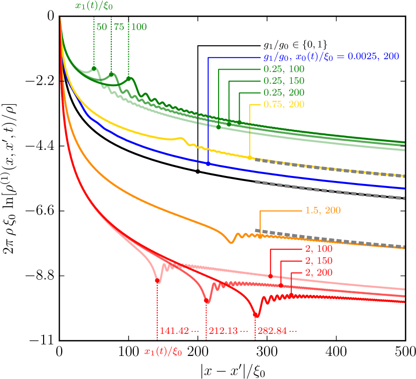
Figure 10: Zero-temperature one-body density matrix $\rho^{(1)}(x,x^{\prime},t)$ for a steplike coupling of the form (82) with $g_{0}\neq 0$, as given in Eq. (117). Different values of the coupling ratio $g_{1}/g_{0}$ and of the dimensionless time $x_{0}(t)/\xi_{0}$ elapsed since $t=0$ are considered. The black curve, obtained for $g_{1}=0$ or $g_{0}$, corresponds to the prequench or the no-quench equilibrium result [first contribution on the right-hand side of Eq. (117)]. The gray dashed curves indicate the long-range behavior (120)–(122) for $g_{1}/g_{0}=0$, 0.75, 1, and 1.5 at $x_{0}(t)/\xi_{0}=200$. The vertical dotted lines indicate the dimensionless “Lieb-Robinson bounds” $x_{1}(t)/\xi_{0}$ [see Eq. (119)] for $g_{1}/g_{0}=0.25$ (green) and $g_{1}/g_{0}=2$ (red) at $x_{0}(t)/\xi_{0}=100$ (light color), $150$ (normal color), and $200$ (dark color).

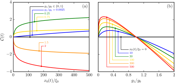
Figure 11: Parameter $\mathcal{C}(t)$, as given by Eq. (122), as a function of the dimensionless time $x_{0}(t)/\xi_{0}$ and for different coupling ratios $g_{1}/g_{0}$ [panel (a)], and as a function of $g_{1}/g_{0}$ for different $x_{0}(t)/\xi_{0}$ [panel (b)]. For $g_{1}=0$ or $g_{0}$ (freezing of the momentum distribution or no quench), one has $\mathcal{C}(t)=0$ [black solid line on (a) and intersection points of the curves on (b)].

The first integral on the right-hand side of Eq. (117) gives the one-body density matrix of the not-yet-quenched system, with constant coupling constant $g_{0}$ Mor03 ; Lar13 . The quench-induced time dependence is embodied in the second contribution. The latter is zero when $g_{1}=0$ or $g_{0}$ which is easily understandable. When $g_{1}=0$, the postquench bosons no longer interact and their $\rho^{(1)}$ function remains frozen to its initial shape. When $g_{1}=g_{0}$, there is no quench at all and the $\rho^{(1)}$ function is the equilibrium one with coupling constant $g_{0}$ at all times. We also understand the sign of this second contribution: When $g_{1}<g_{0}$ ($g_{1}>g_{0}$), the quantum fluctuations are globally reduced (increased) and coherence is accordingly increased (reduced).

At short distances, when $|x-x^{\prime}|$ is much smaller than $\min\{\xi_{0},\xi_{1}\}$, the $\rho^{(1)}$ function is Gaussian, which is typical of noninteracting systems (see, e.g., Ref. Nar99 ). At large distances instead, when $|x-x^{\prime}|$ is much larger than the Lieb-Robinson–type bound

$$x_{1}(t)=2c_{1}t\,,$$ (119)

$\rho^{(1)}$ decays as a power law:

$$\rho^{(1)}(x,x^{\prime},t)\simeq\rho\,\bigg{(}\frac{\exp[2-\gamma+\mathcal{C}(t)]}{4}\,\frac{\xi_{0}}{|x-x^{\prime}|}\bigg{)}^{\alpha}\,.$$ (120)

In this expression, $\gamma=0.57(7)$ is the Euler-Mascheroni constant and the exponent

$$\alpha=\frac{1}{2\pi\rho\xi_{0}}$$ (121)

is exactly the same as the one governing the long-range decay of the prequench, equilibrium one-body density matrix (see, e.g., Refs. Mor03 ; Lar13 ). The time- and coupling-dependent parameter

$$\mathcal{C}(t) \left.=8\,\frac{g_{1}}{g_{0}}\,\bigg{(}1-\frac{g_{1}}{g_{0}}\bigg{)}\right.$$

$$\left.\hphantom{=}\times\int_{0}^{+\infty}dq\,\frac{\displaystyle{\sin^{2}\!\bigg{[}\frac{q}{4}\,\sqrt{q^{2}+4\,\frac{g_{1}}{g_{0}}}\,\frac{x_{0}(t)}{\xi_{0}}\bigg{]}}}{\displaystyle{q\,\bigg{(}q^{2}+4\,\frac{g_{1}}{g_{0}}\bigg{)}\,\sqrt{q^{2}+4}}}\right.$$ (122)

embodies the long-distance effect of the quench. $\mathcal{C}(t)$ is plotted as a function of $x_{0}(t)/\xi_{0}$ for different values of $g_{1}/g_{0}$ in Fig. 11(a), and as a function of $g_{1}/g_{0}$ for different values of $x_{0}(t)/\xi_{0}$ in Fig. 11(b). Note that $\mathcal{C}(t=0)=0$: In this case, the asymptotic behavior (120) of the one-body density matrix is just the prequench one. As expected, $\mathcal{C}(t)$ cancels when $g_{1}=0$ or $g_{0}$ (freezing of the momentum distribution or no quench, respectively); it is positive for $g_{1}<g_{0}$ (since in this case the quench leads to an increased coherence) and negative for $g_{1}>g_{0}$ (decreased coherence). One may also evaluate its large-time [that is, $x_{0}(t)/\xi_{0}\gg 1$] behavior in both limits where $g_{1}$ is very small or very large compared to $g_{0}$. When $g_{1}/g_{0}\ll 1$, we replace $q^{2}+4g_{1}/g_{0}$ with $q^{2}$ in the integrand of Eq. (122) and obtain

$$\mathcal{C}(t)\underset{t\to+\infty}{=}\frac{\pi}{4}\,\frac{g_{1}}{g_{0}}\,\frac{x_{0}(t)}{\xi_{0}}\,.$$ (123)

When $g_{1}/g_{0}\gg 1$ instead, we replace $q^{2}+4g_{1}/g_{0}$ with $4g_{1}/g_{0}$ in the integrand of Eq. (122) and get

$$\mathcal{C}(t)\underset{t\to+\infty}{=}-\frac{1}{2}\,\frac{g_{1}}{g_{0}}\,\bigg{\{}\ln\!\bigg{[}\sqrt{\frac{g_{1}}{g_{0}}}\,\frac{x_{0}(t)}{\xi_{0}}\bigg{]}+2\ln 2+\gamma\bigg{\}}\,.$$ (124)

In the latter expression we kept subdominant contributions in order to have a better approximation of the leading logarithmic term.

The quantity $x_{1}(t)$ introduced in Eq. (119) defines the boundary between the large-distance regime and what is sometimes called the “interior of the light cone.” Its value is indicated in Fig. 10 in units of $\xi_{0}$ for $g_{1}/g_{0}=0.25$ and $g_{1}/g_{0}=2$ at the dimensionless times $x_{0}(t)/\xi_{0}=100$, $150$, and $200$. Dispersive effects are important in our system and the speed of sound $c_{1}$ is not an exact equivalent of the speed of transport of information. As can be seen in Fig. 10, this results in the fact that the separation between the “interior” and the “exterior of the light cone” is not sharp. A hint of the leaking of information “outside of the light cone” is the fact that the parameter $\mathcal{C}(t)$ involved in the long-range behavior of $\rho^{(1)}$ depends on $t$: the correlation between particles separated by a distance exceeding the “Lieb-Robinson bound” $x_{1}(t)$ is affected by the quench.

In the particular case where $g_{0}=0$ and $g_{1}>0$ (not shown in Fig. 10), one has a thermal-like exponential decrease of $\rho^{(1)}$ “within the light cone,” irrespective of whether the system is clean Lar16 or (weakly) disordered Lar18 . No such prethermalization effect is observed in the generic situation where $g_{0}\neq 0$. Note also that, just beyond $x_{1}(t)$, the one-body density matrix displays small-amplitude oscillations. The latter originate from the high-momentum Bogoliubov excitations generated in response to the sudden quench Lar16 .

In Ref. Sch18 , Schemmer et al. consider a thermally occupied initial state. This drastically modifies the long-range behavior of $\rho^{(1)}$, which no longer decays as a power law but exponentially, both before and after the quench. In the large-$|x-x^{\prime}|$ limit, the integral in Eq. (115) is naturally dominated by the infrared contribution. In this phonon limit, the zero-temperature and thermal contributions to the Bogoliubov momentum distribution (116) reduce to

$$n_{k}(t)|_{0} \simeq\frac{1}{2}\,\frac{1+(g_{1}/g_{0}-1)\sin^{2}[k\,x_{1}(t)/2]}{|k|\,\xi_{0}},$$ (125)

$$n_{k}(t)|_{T} \simeq\frac{k_{\mathrm{B}}\,T}{\mu_{0}}\,\frac{1+(g_{1}/g_{0}-1)\sin^{2}[k\,x_{1}(t)/2]}{(k\,\xi_{0})^{2}}\,.$$ (126)

One thus sees that $n_{k}(t)|_{T}$ dominates over $n_{k}(t)|_{0}$ in the $|k|\xi_{0}\ll 1$ regime, which indicates that the long-range $\rho^{(1)}$ function at finite temperature behaves differently from its zero-temperature counterpart. The corresponding Bogoliubov momentum distribution, which is approximately equal to (126), then may be cast in the form

$$n_{k}(t)\simeq\frac{k_{\mathrm{B}}\,T}{\mu_{0}}\,\frac{1}{(k\,\xi_{0})^{2}}+2\,\frac{k_{\mathrm{B}}\,T_{\ast}}{\mu_{0}}\,\frac{\sin^{2}[k\,x_{1}(t)/2]}{(k\,\xi_{0})^{2}}\,,$$ (127)

where we introduced the effective temperature

$$T_{\ast}=\frac{1}{2}\,\bigg{(}\frac{g_{1}}{g_{0}}-1\bigg{)}\,T\,.$$ (128)

Inserting Eq. (127) into Eq. (115) we eventually obtain the following expression for the long-range $\rho^{(1)}$ function:

$$\frac{\rho^{(1)}(x,x^{\prime},t)}{\rho}\simeq\exp\!\left[{-}\pi\,\frac{|x-x^{\prime}|}{\rho\,\Lambda^{2}(T)}-\pi\,\frac{|x-x^{\prime}|}{\rho\,\Lambda^{2}(T_{*})}\right]$$ (129)

when $|x-x^{\prime}|\leqslant x_{1}(t)$, and

$$\frac{\rho^{(1)}(x,x^{\prime},t)}{\rho}\simeq\exp\!\left[{-}\pi\,\frac{|x-x^{\prime}|}{\rho\,\Lambda^{2}(T)}-\pi\,\frac{x_{1}(t)}{\rho\,\Lambda^{2}(T_{*})}\right]$$ (130)

when $|x-x^{\prime}|>x_{1}(t)$. In the two above equations $\Lambda(T)=h(2\pi\,m\,k_{\mathrm{B}}\,T)^{-1/2}$ is the thermal de Broglie wavelength.

As a result, in the very-long-time limit $x_{1}(t)/\xi_{0}\to+\infty$, the long-range $\rho^{(1)}$ function essentially reaches the form expected for a weakly interacting 1D thermal state,

$$\rho^{(1)}(x,x^{\prime},t)\simeq\rho\,\exp\!\bigg{[}{-}\pi\,\frac{|x-x^{\prime}|}{\rho\,\Lambda(T_{\mathrm{fin}})^{2}}\bigg{]}\,,$$ (131)

with a final temperature Sch18

$$T_{\mathrm{fin}}=T+T_{\ast}=\frac{1}{2}\,\bigg{(}1+\frac{g_{1}}{g_{0}}\bigg{)}\,T\,.$$ (132)

We note here that similar results have also been obtained in the theoretical study of a quenched pair of one-dimensional Bose gases within the Luttinger liquid approach Lan18b .

Note that with a $-\pi$ instead of a $-2\pi$ in the argument of the exponential, the long-range, long-time thermal one-body density matrix (131) is very close to that of an ideal gas. The difference is due to the fact that the phase fluctuations are dominant over the density fluctuations in the 1D quasi-ideal regime whereas they equally contribute in the ideal case (see, e.g., Ref. Bou11 ).

V.2 Woods-Saxon-type coupling in 1D

In this section, we consider a situation where the nonlinear coupling constant $g(t)$ obeys a smooth temporal transition from $g_{0}\neq 0$ to $g_{1}\geq 0$ according to the law (92). We assume here that the system is initially in its ground state at $T=0$.

From Eq. (115) and the zero-temperature Bogoliubov momentum distribution (116b) computed using Eqs. (48) and (96), we obtain the following expression for the one-body density matrix at some time $t\geq 0$:

$$\begin{split}2\pi\,\rho\,\xi_{0}\,\ln\!\bigg{[}\frac{\rho^{(1)}(x,x^{\prime},t)}{\rho}\bigg{]}&\left.=-\frac{1}{2}\int_{0}^{+\infty}dq\;\bigg{|}\frac{q-\sqrt{q^{2}+4}}{(q\,\sqrt{q^{2}+4})^{1/2}}\,\frac{{}_{2}F_{1}[\alpha_{q},\gamma_{q}-\beta_{q},\gamma_{q},(1+e^{-t/\tau})^{-1}]}{(1+e^{t/\tau})^{\alpha_{q}}}\right.\\ &\left.\hphantom{=}+2\,\bigg{(}\frac{\sqrt{q^{2}+4}}{q}\bigg{)}^{1/2}\,\frac{\alpha_{q}\,\beta_{q}}{(\alpha_{q}+\beta_{q})\,\gamma_{q}}\,\frac{{}_{2}F_{1}[\alpha_{q}+1,\gamma_{q}-\beta_{q},\gamma_{q}+1,(1+\mathrm{e}^{-t/\tau})^{-1}]\,e^{t/\tau}}{(1+e^{t/\tau})^{\alpha_{q}+1}}\bigg{|}^{2}\right.\\ &\left.\hphantom{=}\times\bigg{[}1-\cos\!\bigg{(}q\,\frac{|x-x^{\prime}|}{\xi_{0}}\bigg{)}\bigg{]}\,,\right.\end{split}$$

where, from Eqs. (95),

$$\alpha_{q} \left.=-i\,\frac{q}{4}\,\bigg{(}\sqrt{q^{2}+4}\,-\sqrt{q^{2}+4\,\frac{g_{1}}{g_{0}}}\bigg{)}\,\frac{x_{0}(\tau)}{\xi_{0}}\,,\right.$$ (133a)

$$\beta_{q} \left.=-i\,\frac{q}{4}\,\bigg{(}\sqrt{q^{2}+4}\,+\sqrt{q^{2}+4\,\frac{g_{1}}{g_{0}}}\bigg{)}\,\frac{x_{0}(\tau)}{\xi_{0}}\,,\right.$$ (133b)

$$\gamma_{q} \left.=1-i\,\frac{q}{2}\,\sqrt{q^{2}+4}\;\frac{x_{0}(\tau)}{\xi_{0}}\,.\right.$$ (133c)

The corresponding $\rho^{(1)}$ is plotted in Fig. 12 as a function of $|x-x^{\prime}|/\xi_{0}$ for $x_{0}(\tau)/\xi_{0}=10$ and for several values of $g_{1}/g_{0}$ and $x_{0}(t)/\xi_{0}$.

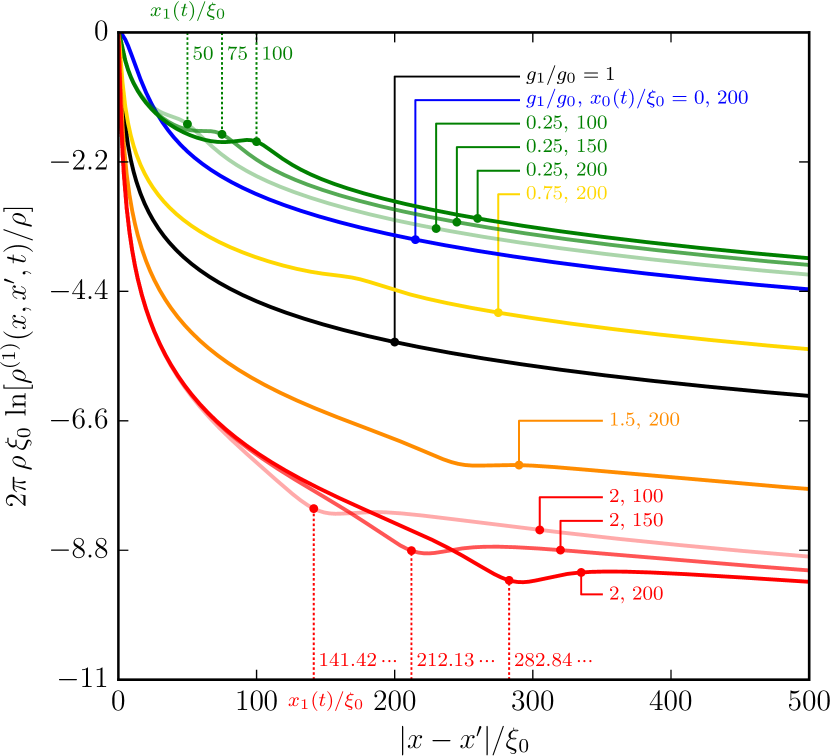
Figure 12: Same as Fig. 10 for a Woods-Saxon-type coupling of the form (92) with $x_{0}(\tau)/\xi_{0}=0$, as given in Eqs. (V.2). The black curve, obtained for $g_{1}=g_{0}$, corresponds to the no-quench equilibrium result.

As in the case of a steplike quench in $g(t)$, the long-range $\rho^{(1)}$ function presents a power-law decay roughly of the form (120). In the present case, contrarily to what has been done in Eq. (122), an analytic expression for $\mathcal{C}(t)$ is not easily obtained, but one may show by detailed numerical inspection that the exponent $\alpha$ which governs the large-distance power-law decrease of the zero-temperature $\rho^{(1)}$ is the same as the one given in Eq. (121), which governs the long-range behavior of the prequench one-body density matrix. Also in the present case, the regular and continuous time dependence of the coupling parameter smooths out the oscillations observed around the Lieb-Robinson bound $x_{1}(t)$ for the steplike-quench one-body density matrix (compare Figs. 10 and 12).

Similar results have been obtained in Ref. Ber14 in the framework of Luttinger liquid description for a piecewise linear function $g(t)$. In this reference, as in the present work, the light-cone effect is less marked than for an abrupt quench and accompanied by no oscillations in $\rho^{(1)}$. Here, however, at variance with Ref. Ber14 , we do not need to introduce an effective Lieb-Robinson bound for a correct description of the transition between short- and long-distance behavior.

VI Conclusion

We have analyzed some of the most relevant properties of a weakly interacting uniform Bose gas having a time-varying coupling strength. In three dimensions the system can be considered as a condensate (which can be described within a mean-field approach) with small additional quantum fluctuations. These can be treated within a time-dependent Bogoliubov framework, that enables one to determine the time evolution of any observable. One gets a useful physical insight into the problem by viewing each excited mode as a time-dependent harmonic oscillator, whose frequency coincides with the instantaneous Bogoliubov one. Using this correspondence, we prove some general properties, such as the freezing of the low-momentum modes, the adiabatic behavior of the high-momentum ones, and the possible occurrence of Sakharov oscillations at large evolution times. It would be interesting to also use the gravitational analogy to study temporal evolutions relevant in cosmology; work in this direction is in progress.

Additionally, by mapping the problem onto a scattering one, we identified a few families of time-dependent couplings whose evolution equations can be solved analytically. For these models, we calculate the quantum depletion (in three dimensions) and the full one-body density matrix (in one dimension), that characterize the degree of coherence of the system. In the one-dimensional case our results point to the absence of prethermalization for a typical quench protocol when the Bose gas is initially interacting and at zero temperature. On the other hand, at finite initial temperature, the density matrix evolves to a configuration typical for a new thermal state Sch18 .

Appendix A Change of initial time

Let us assume that we know the solution $\gamma_{k}(t,t_{0})$ of the TDHO equation (51) for a given initial time $t_{0}$, and that we want to calculate $\gamma_{k}(t,t_{0}^{\prime})$ with $t_{0}^{\prime}>t_{0}$. Evidently, for $t\leq t_{0}^{\prime}$ one has $\gamma_{k}(t,t_{0}^{\prime})=\exp[-i\omega_{k}(t_{0}^{\prime})(t-t_{0}^{\prime})]$. For $t>t_{0}^{\prime}$ one can express $\gamma_{k}(t,t_{0}^{\prime})$ as a linear combination of $\gamma_{k}(t,t_{0})$ and $\gamma_{k}^{*}(t,t_{0})$. The coefficients of the combination are set by the requirement that $\gamma_{k}(t,t_{0}^{\prime})$ and its first-order derivative be continuous at $t=t_{0}^{\prime}$. By doing this, one ends up with the expression (valid for $t>t_{0}^{\prime}$)

$$\begin{split}\gamma_{k}(t,t_{0}^{\prime})={}&{}\sqrt{\frac{\omega_{k}(t_{0}^{\prime})}{\omega_{k}(t_{0})}}\\ {}&{}\times\left[\beta_{1,k}^{*}(t^{\prime}_{0},t_{0})\gamma_{k}(t,t_{0})-\beta_{2,k}(t_{0}^{\prime},t_{0})\gamma_{k}^{*}(t,t_{0})\right]\,.\end{split}$$ (134)

Here, the two quantities $\beta_{1,k}(t_{0}^{\prime},t_{0})$ and $\beta_{2,k}(t_{0}^{\prime},t_{0})$ are given by

$$\beta_{1,k}(t_{0}^{\prime},t_{0})+\beta_{2,k}(t_{0}^{\prime},t_{0}) {}=\sqrt{\frac{\omega_{k}(t_{0}^{\prime})}{\omega_{k}(t_{0})}}\,\gamma_{k}(t_{0}^{\prime},t_{0})\,,$$ (135a)

$$\beta_{1,k}(t_{0}^{\prime},t_{0})-\beta_{2,k}(t_{0}^{\prime},t_{0}) {}=\sqrt{\frac{\omega_{k}(t_{0})}{\omega_{k}(t_{0}^{\prime})}}\,\tilde{\gamma}_{k}(t_{0}^{\prime},t_{0})\,.$$ (135b)

They coincide with the entries of the quasiparticle propagator (23) calculated at $t=t_{0}^{\prime}$. This can be verified, for instance, starting from Eqs. (27) and expressing $\beta_{1,k}(t,t_{0})$ and $\beta_{2,k}(t,t_{0})$ in terms of $U_{k}(t,t_{0})$ and $V_{k}(t,t_{0})$. Then, combining the result with Eqs. (48) and setting $t=t_{0}^{\prime}$, one gets the relations (135).

The large-$t$ behavior of $\gamma_{k}(t,t_{0}^{\prime})$ can be found from that of $\gamma_{k}(t,t_{0})$ given by Eq. (74). One finds

$$\begin{split}\gamma_{k}(t,t_{0}^{\prime})\underset{t\to+\infty}{=}{}&{}e^{i\omega_{k}(t_{0}^{\prime})t_{0}^{\prime}}\sqrt{\frac{\omega_{k}(t_{0}^{\prime})}{\omega_{k}(+\infty)}}\\ {}&{}\times\left[\tau^{\leftarrow}_{k}(t_{0}^{\prime})e^{-i\omega_{k}(+\infty)t}+\tau^{\leftarrow}_{k}(t_{0}^{\prime})e^{i\omega_{k}(+\infty)t}\right]\,,\end{split}$$ (136)

where the transfer coefficients at the new initial time $t_{0}^{\prime}$ are

$$\begin{split}\tau^{\leftarrow}_{k}(t_{0}^{\prime})={}&{}e^{i[\omega_{k}(t_{0})t_{0}-\omega_{k}(t_{0}^{\prime})t_{0}^{\prime}]}\\ &{}\times\left[\beta_{1,k}^{*}(t_{0}^{\prime},t_{0})\tau^{\leftarrow}_{k}(t_{0})-\beta_{2,k}(t_{0}^{\prime},t_{0})\tau^{\rightarrow}_{k}(t_{0})\right]\,,\end{split}$$ (137a)

$$\begin{split}\tau^{\rightarrow}_{k}(t_{0}^{\prime})={}&{}e^{i[\omega_{k}(t_{0})t_{0}-\omega_{k}(t_{0}^{\prime})t_{0}^{\prime}]}\\ &{}\times\left[\beta_{1,k}^{*}(t_{0}^{\prime},t_{0})\tau^{\rightarrow}_{k}(t_{0})-\beta_{2,k}(t_{0}^{\prime},t_{0})\tau^{\leftarrow}_{k}(t_{0})\right]\,.\end{split}$$ (137b)

Appendix B Proof of the constancy of the asymptotic value of the condensate depletion

The starting point is the asymptotic expression (77) of the momentum distribution, which we rewrite expanding the square modulus:

$$\begin{split}n_{\mathbf{k}}(t)\underset{t\to+\infty}{=}{}&|v_{k}(+\infty)\tau^{\leftarrow}_{k}(t_{0})|^{2}+|u_{k}(+\infty)\tau^{\rightarrow}_{k}(t_{0})|^{2}\\ &{}+2u_{k}(+\infty)v_{k}(+\infty)\\ &\phantom{{}+}\times\operatorname{Re}\left[\tau^{\leftarrow}_{k}(t_{0})\tau^{\rightarrow*}_{k}(t_{0})e^{-2i\omega_{k}(+\infty)t}\right]\,.\end{split}$$ (138)

Integrating both sides of this equality over the whole momentum space one reproduces Eq. (80), provided that the integral of the third term on the right-hand side vanishes for $t\to+\infty$. This statement is trivially true if $g(+\infty)=0$ because $v_{k}(+\infty)=0$. Therefore, we need to prove that it also remains valid when $g(+\infty)\neq 0$. Let us then try to evaluate

$$\begin{split}&\int d^{3}k\,u_{k}(+\infty)v_{k}(+\infty)\tau^{\leftarrow}_{k}(t_{0})\tau^{\rightarrow*}_{k}(t_{0})e^{-2i\omega_{k}(+\infty)t}\\ &{}=-2\pi\int_{0}^{+\infty}\!\!\!\!\!\!dk\,k^{2}\frac{g(+\infty)\rho}{\hbar\omega_{k}(+\infty)}\tau^{\leftarrow}_{k}(t_{0})\tau^{\rightarrow*}_{k}(t_{0})e^{-2i\omega_{k}(+\infty)t}\,.\end{split}$$ (139)

Here, we have performed the trivial integration over the solid angle and we have used the explicit formulas (13) for the instantaneous Bogoliubov weights. It is convenient to change the integration variable to $\eta=\omega_{k}(+\infty)t$. The Bogoliubov dispersion (14) can be easily inverted to express $k$ as a function of $\eta/t$. We get

$$k=\xi^{-1}(+\infty)\sqrt{2[(1+\eta^{2}/\tilde{t}^{2})^{1/2}-1]}\,,$$ (140)

where $\tilde{t}=g(+\infty)\rho t/\hbar$ is a dimensionless time variable. Then, Eq. (139) can be rewritten as $-2\sqrt{2}\pi\xi^{-3}(+\infty)\int_{0}^{+\infty}d\eta\,F(\eta,\tilde{t})\,e^{-2i\eta}$, where

$$\begin{split}F(\eta,\tilde{t})={}&{}\frac{1}{(1+\eta^{2}/\tilde{t}^{2})^{1/2}}\left[\frac{(1+\eta^{2}/\tilde{t}^{2})^{1/2}-1}{\tilde{t}^{2}}\right]^{1/2}\\ &{}\times\tau^{\leftarrow}_{\eta/\tilde{t}}(t_{0})\tau^{\rightarrow*}_{\eta/\tilde{t}}(t_{0})\,.\end{split}$$ (141)

We notice that the first factor in the right-hand size of Eq. (141) tends to $1$ as $\tilde{t}\to+\infty$, whereas the second one behaves like $\eta/\sqrt{2}\tilde{t}^{2}$. It remains to understand what happens to the transfer coefficients $\tau^{\leftarrow}_{\eta/\tilde{t}}(t_{0})$ and $\tau^{\rightarrow*}_{\eta/\tilde{t}}(t_{0})$ in this limit. To this purpose, we make use of the relations

$$\begin{split}\tau^{\leftarrow}_{k}(t_{0})={}&{}\lim_{t\to+\infty}\Bigg{\{}e^{-i\omega_{k}(t_{0})t_{0}}e^{i\omega_{k}(+\infty)t}\\ &{}\times\frac{1}{2}\left[\sqrt{\frac{\omega_{k}(+\infty)}{\omega_{k}(t_{0})}}\,\gamma_{k}(t,t_{0})+\sqrt{\frac{\omega_{k}(t_{0})}{\omega_{k}(+\infty)}}\,\tilde{\gamma}_{k}(t,t_{0})\right]\Bigg{\}}\,,\end{split}$$ (142a)

$$\begin{split}\tau^{\rightarrow}_{k}(t_{0})={}&{}\lim_{t\to+\infty}\Bigg{\{}e^{-i\omega_{k}(t_{0})t_{0}}e^{-i\omega_{k}(+\infty)t}\\ &{}\times\frac{1}{2}\left[\sqrt{\frac{\omega_{k}(+\infty)}{\omega_{k}(t_{0})}}\,\gamma_{k}(t,t_{0})-\sqrt{\frac{\omega_{k}(t_{0})}{\omega_{k}(+\infty)}}\,\tilde{\gamma}_{k}(t,t_{0})\right]\Bigg{\}}\,.\end{split}$$ (142b)

Equations (142) follow from the asymptotic expressions of $\gamma_{k}$ [see Eq. (74)] and $\tilde{\gamma}_{k}$ (easily deduced from that of $\gamma_{k}$). In Sec. III.2 we have seen that, if $g(t_{0})\neq 0$, then $\gamma_{k}(t,t_{0})\to 1$ and $\tilde{\gamma}_{k}(t,t_{0})\to 1$ for $k\to 0$. This yields

$$\tau^{\leftarrow}_{k}(t_{0})\tau^{\rightarrow*}_{k}(t_{0})\underset{k\to 0}{=}\frac{1}{4}\left[\sqrt{\frac{g(+\infty)}{g(t_{0})}}-\sqrt{\frac{g(t_{0})}{g(+\infty)}}\right]\,.$$ (143)

Instead, if $g(t_{0})=0$, at low $k$ one has $\gamma_{k}(t,t_{0})\to 1$, $\tilde{\gamma}_{k}(t,t_{0})\to Z(t,t_{0})$ [with $Z$ given by Eq. (57)], and

$$\tau^{\leftarrow}_{k}(t_{0})\tau^{\rightarrow*}_{k}(t_{0})\underset{k\to 0}{=}\frac{mc(+\infty)}{2\hbar k}\,.$$ (144)

Thus, we find that in the $\tilde{t}\to+\infty$ limit the product $\tau^{\leftarrow}_{\eta/\tilde{t}}(t_{0})\tau^{\rightarrow*}_{\eta/\tilde{t}}(t_{0})$ approaches a finite value if $g(t_{0})\neq 0$, while it behaves like $\tilde{t}/2\eta$ if $g(t_{0})=0$. In both cases $F(\eta,\tilde{t})$ vanishes at large times, and so does its integral over $\eta$. Hence, we conclude that the time-dependent terms in Eq. (138) do not contribute to the total depletion at $t\to+\infty$.

Appendix C Analytic continuation of hypergeometric functions

The hypergeometric function is usually defined as the sum of the power series Abr65

$${}_{2}F_{1}(a,b,c;z)=\sum_{n=0}^{+\infty}\frac{(a)_{n}(b)_{n}}{(c)_{n}}\frac{z^{n}}{n!}\,,$$ (145)

where $(a)_{n}=\Gamma(a+n)/\Gamma(a)$ is the Pochhammer symbol. This power series converges only if $|z|<1$. However, the hypergeometric function can be analytically continued along any path in the complex plane that avoids the branch points $z=1$ and $\infty$. For instance, in Sec. IV.2 we had to consider hypergeometric functions with real negative argument. One can deal with such a situation by resorting to the Pfaff transformations

$${}_{2}F_{1}(a,b,c;z) {}=(1-z)^{-a}{}_{2}F_{1}(a,c-b,c;\textstyle\frac{z}{z-1})\,,$$ (146a)

$${}_{2}F_{1}(a,b,c;z) {}=(1-z)^{-b}{}_{2}F_{1}(c-a,b,c;\textstyle\frac{z}{z-1})\,.$$ (146b)

These identities hold where the domains of the functions on both sides overlap. If $|z|\geq 1$ and $\operatorname{Re}z<1/2$, Eqs. (146) define the analytic continuation of the hypergeometric function to this latter domain, where the right-hand side is well defined. An additional advantage of Eqs. (146) is that they provide a more efficient way to compute numerically the hypergeometric function for negative argument. Indeed, since $\left|\frac{z}{z-1}\right|<|z|$ when $z<0$, the power series expansions (145) of the functions on the right-hand side converge faster than that of ${}_{2}F_{1}(a,b,c;z)$. The composition of the two Pfaff transformations yields the Euler transformation

$${}_{2}F_{1}(a,b,c;z)=(1-z)^{c-a-b}{}_{2}F_{1}(c-a,c-b,c;z)\,.$$ (147)

There are many other identities in literature that allow one to establish the analytic continuation of the hypergeometric function Abr65 . Among these we mention the following:

$$\begin{split}{}_{2}F_{1}(a,b,c;z)={}&\frac{\Gamma(c)\Gamma(b-a)}{\Gamma(b)\Gamma(c-a)}(-z)^{-a}\\ &\times{}_{2}F_{1}(a,1-c+a,1-b+a;z^{-1})\\ &{}+\frac{\Gamma(c)\Gamma(a-b)}{\Gamma(a)\Gamma(c-b)}(-z)^{-b}\\ &\times{}_{2}F_{1}(b,1-c+b,1-a+b;z^{-1})\,,\end{split}$$ (148a)

$$\begin{split}{}_{2}F_{1}(a,b,c;z)={}&\frac{\Gamma(c)\Gamma(c-a-b)}{\Gamma(c-a)\Gamma(c-b)}\\ &\times{}_{2}F_{1}(a,b,a+b-c+1;1-z)\\ &{}+\frac{\Gamma(c)\Gamma(a+b-c)}{\Gamma(a)\Gamma(b)}(1-z)^{c-a-b}z^{1-c}\\ &\times{}_{2}F_{1}(1-b,1-a,c-a-b+1;1-z)\,.\end{split}$$ (148b)

Equations (148a) and (148b) are used in Secs. IV.2 and IV.3, respectively, to analytically extend the solutions of the TDHO equation for the Woods-Saxon and the modified Pöschl-Teller couplings. They are especially useful for extrapolating the large-$t$ behavior, yielding the transfer coefficients. Notice that, strictly speaking, the domains of the hypergeometric functions on the two sides of the identity (148a) do not overlap: the left-hand side is defined for $|z|<1$, the right-hand side for $|z|>1$. In writing this formula we implicitly assume that an intermediate analytic continuation around $z=-1$ is made, e.g., through the Pfaff transformations (146). Concerning Eq. (148b), both sides are simultaneously defined for $0<z<1$, hence, there is no need for intermediate continuations.

References

- (1) M. H. Anderson, J. R. Ensher, M. R. Matthews, C. E. Wieman, and E. A. Cornell, Science 269, 198 (1995), doi:10.1126/science.269.5221.198.
- (2) K. B. Davis, M.-O. Mewes, M. R. Andrews, N. J. van Druten, D. S. Durfee, D. M. Kurn, and W. Ketterle, Phys. Rev. Lett. 75, 3969 (1995), doi:10.1103/PhysRevLett.75.3969.
- (3) M. Kozuma, L. Deng, E. W. Hagley, J. Wen, R. Lutwak, K. Helmerson, S. L. Rolston, and W. D. Phillips, Phys. Rev. Lett. 82, 871 (1999), doi:10.1103/PhysRevLett.82.871.
- (4) D. M. Stamper-Kurn, A. P. Chikkatur, A. Görlitz, S. Inouye, S. Gupta, D. E. Pritchard, and W. Ketterle, Phys. Rev. Lett. 83, 2876 (1999), doi:10.1103/PhysRevLett.83.2876.
- (5) J. Steinhauer, R. Ozeri, N. Katz, and N. Davidson, Phys. Rev. Lett. 88, 120407 (2002), doi:10.1103/PhysRevLett.88.120407.
- (6) R. Ozeri, N. Katz, J. Steinhauer, and N. Davidson, Rev. Mod. Phys. 77, 187 (2005), doi:10.1103/RevModPhys.77.187.
- (7) C. Tozzo and F. Dalfovo, Phys. Rev. A 69, 053606 (2004), doi:10.1103/PhysRevA.69.053606.
- (8) R. Lopes, C. Eigen, N. Navon, D. Clément, R. P. Smith, and Z. Hadzibabic, Phys. Rev. Lett. 119, 190404 (2017), doi:10.1103/PhysRevLett.119.190404.
- (9) R. Chang, Q. Bouton, H. Cayla, C. Qu, A. Aspect, C. I. Westbrook, and D. Clément, Phys. Rev. Lett. 117, 235303 (2016), doi:10.1103/PhysRevLett.117.235303.
- (10) R. A. Duine and H. T. C. Stoof, arXiv:cond-mat/0204529.
- (11) D. J. Papoular, L. P. Pitaevskii, and S. Stringari, Phys. Rev. A 94, 023622 (2016), doi:10.1103/PhysRevA.94.023622.
- (12) A. Fabbri and N. Pavloff, SciPost Phys. 4, 019 (2018), doi:10.21468/SciPostPhys.4.4.019.
- (13) P. O. Fedichev and U. R. Fischer, Phys. Rev. A 69, 033602 (2004), doi:10.1103/PhysRevA.69.033602.
- (14) M. Uhlmann, Y. Xu, and R. Schützhold, New J. Phys. 7, 248 (2005), doi:10.1088/1367-2630/7/1/248.
- (15) M. Uhlmann, Phys. Rev. A 79, 033601 (2009), doi:10.1103/PhysRevA.79.033601.
- (16) A. Imambekov, I. E. Mazets, D. S. Petrov, V. Gritsev, S. Manz, S. Hofferberth, T. Schumm, E. Demler, and J. Schmiedmayer, Phys. Rev. A 80, 033604 (2009), doi:10.1103/PhysRevA.80.033604.
- (17) C.-L. Hung, V. Gurarie, and C. Chin, Science 341, 1213 (2013), doi:10.1126/science.1237557.
- (18) S. Eckel, A. Kumar, T. Jacobson, I. B. Spielman, and G. K. Campbell, Phys. Rev. X 8, 021021 (2018), doi:10.1103/PhysRevX.8.021021.
- (19) I. Carusotto, R. Balbinot, A. Fabbri, and A. Recati, Eur. Phys. J. D 56, 391 (2010), doi:10.1140/epjd/e2009-00314-3.
- (20) J.-C. Jaskula, G. B. Partridge, M. Bonneau, R. Lopes, J. Ruaudel, D. Boiron, and C. I. Westbrook, Phys. Rev. Lett. 109, 220401 (2012), doi:10.1103/PhysRevLett.109.220401.
- (21) X. Busch, I. Carusotto, and R. Parentani, Phys. Rev. A 89, 043819 (2014), doi:10.1103/PhysRevA.89.043819.
- (22) S. Robertson, F. Michel, and R. Parentani, Phys. Rev. D 95, 065020 (2017), doi:10.1103/PhysRevD.95.065020.
- (23) S. Robertson, F. Michel, and R. Parentani, Phys. Rev. D 96, 045012 (2017), doi:10.1103/PhysRevD.96.045012.
- (24) S. Ghosh, K. S. Gupta, and S. C. L. Srivastava, EPL 120, 50005 (2017), doi:10.1209/0295-5075/120/50005.
- (25) Z. Tian, S.-Y. Chä, and U. R. Fischer, Phys. Rev. A 97, 063611 (2018), doi:10.1103/PhysRevA.97.063611.
- (26) M. Cheneau, P. Barmettler, D. Poletti, M. Endres, P. Schauß, T. Fukuhara, C. Gross, I. Bloch, C. Kollath, and S. Kuhr, Nature (London) 481, 484 (2012), doi:10.1038/nature10748.
- (27) S. Trotzky, Y-A. Chen, A. Flesch, I. P. McCulloch, U. Schollwöck, J. Eisert, and I. Bloch, Nature Phys. 8, 325 (2012), doi:10.1038/nphys2232.
- (28) M. Gring, M. Kuhnert, T. Langen, T. Kitagawa, B. Rauer, M. Schreitl, I. Mazets, D. Adu Smith, E. Demler, and J. Schmiedmayer, Science 337, 1318 (2012), doi:10.1126/science.1224953.
- (29) T. Langen, R. Geiger, M. Kuhnert, B. Rauer, and J. Schmiedmayer, Nature Phys. 9, 640 (2013), doi:10.1038/nphys2739.
- (30) G. Menegoz and A. Silva, J. Stat. Mech. (2015) P05035, doi:10.1088/1742-5468/2015/05/P05035.
- (31) P.-É. Larré and I. Carusotto, Eur. Phys. J. D 70, 45 (2016), doi:10.1140/epjd/e2016-60590-2.
- (32) M. Buchhold, M. Heyl, and S. Diehl, Phys. Rev. A 94, 013601 (2016), doi:10.1103/PhysRevA.94.013601.
- (33) M. Schemmer, A. Johnson, and I. Bouchoule, Phys. Rev. A 98, 043604 (2018), doi:10.1103/PhysRevA.98.043604.
- (34) X. Yin and L. Radzihovsky, Phys. Rev. A 88, 063611 (2013), doi:10.1103/PhysRevA.88.063611.
- (35) P. Makotyn, C. E. Klauss, D. L. Goldberger, E. A. Cornell, and D. S. Jin, Nature Phys. 10, 114 (2014), doi:10.1038/nphys2850.
- (36) A. G. Sykes, J. P. Corson, J. P. D’Incao, A. P. Koller, C. H. Greene, A. M. Rey, K. R. A. Hazzard, and J. L. Bohn, Phys. Rev. A 89, 021601(R) (2014), doi:10.1103/PhysRevA.89.021601.
- (37) C. Eigen, J. A. P. Glidden, R. Lopes, E. A. Cornell, R. P. Smith, Z. Hadzibabic, Nature (London) 563, 221 (2018), doi:10.1038/s41586-018-0674-1.
- (38) C. Qu, L. P. Pitaevskii, and S. Stringari, Phys. Rev. A 94, 063635 (2016), doi:10.1103/PhysRevA.94.063635.
- (39) L. W. Clark, A. Gaj, L. Feng, and C. Chin, Nature (London) 551, 356 (2017), doi:10.1038/nature24272.
- (40) N. Goldman, J. Dalibard, M. Aidelsburger, and N. R. Cooper, Phys. Rev. A 91, 033632 (2015), doi:10.1103/PhysRevA.91.033632.
- (41) F. Meinert, M. J. Mark, K. Lauber, A. J. Daley, and H.-C. Nägerl, Phys. Rev. Lett. 116, 205301 (2016), doi:10.1103/PhysRevLett.116.205301.
- (42) N. Fläschner, B. S. Rem, M. Tarnowski, D. Vogel, D. S. Lühmann, K. Sengstock, and C. Weitenberg, Science 352, 1091 (2016), doi:10.1126/science.aad4568.
- (43) K. Plekhanov, G. Roux, and K. Le Hur, Phys. Rev. B 95, 045102 (2017), doi:10.1103/PhysRevB.95.045102.
- (44) L. W. Clark, B. M. Anderson, L. Feng, A. Gaj, K. Levin, and C. Chin, Phys. Rev. Lett. 121, 030402 (2018), doi:10.1103/PhysRevLett.121.030402.
- (45) A. G. Sykes, H. Landa, and D. S. Petrov, Phys. Rev. A 95, 062705 (2017), doi:10.1103/PhysRevA.95.062705.
- (46) H. Landa, Phys. Rev. A 97, 042705 (2018), doi:10.1103/PhysRevA.97.042705.
- (47) J.-S. Bernier, G. Roux, and C. Kollath, Phys. Rev. Lett. 106, 200601 (2011), doi:10.1103/PhysRevLett.106.200601.
- (48) A. U. J. Lode, K. Sakmann, O. E. Alon, L. S. Cederbaum, and A. I. Streltsov, Phys. Rev. A 86, 063606 (2012), doi:10.1103/PhysRevA.86.063606.
- (49) P. Ziń and M. Pylak, J. Phys. B: At. Mol. Opt. Phys. 50, 085301 (2017), doi:10.1088/1361-6455/aa65ad.
- (50) M. Van Regemortel, H. Kurkjian, I. Carusotto, and M. Wouters, Phys. Rev. A 98, 053612 (2018), doi:10.1103/PhysRevA.98.053612.
- (51) M. Pylak and P. Ziń, Phys. Rev. A 98, 043603 (2018), doi:10.1103/PhysRevA.98.043603.
- (52) S. Robertson, F. Michel, and R. Parentani, Phys. Rev. D 98, 056003 (2018), doi:10.1103/PhysRevD.98.045012.
- (53) A. L. Gaunt, T. F. Schmidutz, I. Gotlibovych, R. P. Smith, and Z. Hadzibabic, Phys. Rev. Lett. 110, 200406 (2013), doi:10.1103/PhysRevLett.110.200406.
- (54) L. P. Pitaevskii and S. Stringari, Bose-Einstein Condensation and Superfluidity (Oxford University Press, Oxford, 2016).
- (55) J. P. Corson and J. L. Bohn, Phys. Rev. A 91, 013616 (2015), doi:10.1103/PhysRevA.91.013616.
- (56) J. P. Corson and J. L. Bohn, Phys. Rev. A 94, 023604 (2016), doi:10.1103/PhysRevA.94.023604.
- (57) V. E. Colussi, J. P. Corson, and J. P. D’Incao, Phys. Rev. Lett 120, 100401 (2018), doi:10.1103/PhysRevLett.120.100401.
- (58) V. N. Popov, Theor. Math. Phys. 11, 565 (1972), doi:10.1007/BF01028373.
- (59) V. N. Popov, Functional Integrals in Quantum Field Theory and Statistical Physics (Reidel, Dordrecht, 1983).
- (60) C. Mora and Y. Castin, Phys. Rev. A 67, 053615 (2003), doi:10.1103/PhysRevA.67.053615.
- (61) P.-É. Larré, Quantum fluctuations and nonlinear effects in Bose-Einstein condensates: From dispersive shock waves to acoustic Hawking radiation, Ph.D. thesis, University of Paris-Sud, 2013.
- (62) T. D. Lee, K. Huang, and C. N. Yang, Phys. Rev. 106, 1135 (1957), doi:10.1103/PhysRev.106.1135.
- (63) R. M. Kulsrud, Phys. Rev. 106, 205 (1957), doi:10.1103/PhysRev.106.205.
- (64) H. R. Lewis, Jr., Phys. Rev. Lett. 18, 510 (1967), doi:10.1103/PhysRevLett.18.510.
- (65) L. D. Landau and E. M. Lifshitz, Quantum Mechanics – Non-relativistic Theory, 3rd edn. (Pergamon Press, Oxford, 1977).
- (66) A. D. Sakharov, Zh. Eksp. Teor. Fiz. 49, 345 (1965) [Sov. Phys.-JETP 22, 241 (1966)].
- (67) L. P. Grishchuk, Phys.-Usp. 55, 210 (2012), doi:10.3367/UFNe.0182.201202l.0222.
- (68) J.-S. Bernier, R. Citro, C. Kollath, and E. Orignac, Phys. Rev. Lett. 112, 065301 (2014), doi:10.1103/PhysRevLett.112.065301.
- (69) M. Abramowitz and I. A. Stegun, Handbook of Mathematical Functions with Formulas, Graphs, and Mathematical Tables (Dover Publications, New York, 1965).
- (70) F. Dalfovo, S. Giorgini, L. P. Pitaevskii, and S. Stringari, Rev. Mod. Phys. 71, 463 (1999), doi:10.1103/RevModPhys.71.463.
- (71) P.-É. Larré, D. Delande, and N. Cherroret, Phys. Rev. A 97, 043805 (2018), doi:10.1103/PhysRevA.97.043805.
- (72) N. D. Mermin and H. Wagner, Phys. Rev. Lett. 17, 1133 (1966), doi:10.1103/PhysRevLett.17.1133.
- (73) P. C. Hohenberg, Phys. Rev. 158, 383 (1967), doi:10.1103/PhysRev.158.383.
- (74) L. P. Pitaevskii and S. Stringari, J. Low Temp. Phys. 85, 377 (1991), doi:10.1007/BF00682193.
- (75) U. R. Fischer, Phys. Rev. Lett. 89, 280402 (2002), doi:10.1103/PhysRevLett.89.280402.
- (76) V. Gritsev, T. Rostunov, and E. Demler, J. Stat. Mech. (2010) P05012, doi:10.1088/1742-5468/2010/05/P05012.
- (77) M. Kormos, M. Collura, and P. Calabrese, Phys. Rev. A 89, 013609 (2014), doi:10.1103/PhysRevA.89.013609.
- (78) L. Foini, A. Gambassi, R. Konik, and L. F. Cugliandolo, Phys. Rev. E 95, 052116 (2017), doi:10.1103/PhysRevE.95.052116.
- (79) J. De Nardis, B. Wouters, M. Brockmann, and J.-S. Caux, Phys. Rev. A 89, 033601 (2014), doi:10.1103/PhysRevA.89.033601.
- (80) L. Piroli, P. Calabrese, and F. H. L. Essler, SciPost Phys. 1, 001 (2016), doi:10.21468/SciPostPhys.1.1.001.
- (81) M. Olshanii, Phys. Rev. Lett. 81, 938 (1998), doi:10.1103/PhysRevLett.81.938.
- (82) M. Naraschewski and R. J. Glauber, Phys. Rev. A 59, 4595 (1999), doi:10.1103/PhysRevA.59.4595.
- (83) T. Langen, T. Schweigler, E. Demler, and J. Schmiedmayer, New J. Phys. 20, 023034 (2018), doi:10.1088/1367-2630/aaaaa5.
- (84) I. Bouchoule, N. J. Van Druten, and C. I. Westbrook, in Atom Chips, edited by J. Reichel and V. Vuletić (Wiley Online Library, 2011).