Covariate Distribution Balance via Propensity Scores

Abstract

This paper proposes new estimators for the propensity score that aim to maximize the covariate distribution balance among different treatment groups. Heuristically, our proposed procedure attempts to estimate a propensity score model by making the underlying covariate distribution of different treatment groups as close to each other as possible. Our estimators are data-driven, do not rely on tuning parameters such as bandwidths, admit an asymptotic linear representation, and can be used to estimate different treatment effect parameters under different identifying assumptions, including unconfoundedness and local treatment effects. We derive the asymptotic properties of inverse probability weighted estimators for the average, distributional, and quantile treatment effects based on the proposed propensity score estimator and illustrate their finite sample performance via Monte Carlo simulations and two empirical applications.

1 Introduction

Identifying and estimating the effect of a policy, treatment or intervention on an outcome of interest is one of the main goals in applied research. Although a randomized control trial (RCT) is the gold standard to identify causal effects, many times its implementation is infeasible and researchers have to rely on observational data. In such settings, the propensity score (PS), which is defined as the probability of being treated given observed covariates, plays a prominent role. Statistical methods using the PS include matching, inverse probability weighting (IPW), regression, as well as combinations thereof; for review, see, e.g., Imbens2015.

To use these methods in practice, one has to acknowledge that the PS is usually unknown and has to be estimated from the observed data. Given the moderate or high dimensionality of available covariates, researchers are usually coerced to adopt a parametric model for the PS. A popular approach is to assume a linear logistic model, estimate the unknown parameters by maximum likelihood (ML), check if the resulting PS estimates balance specific moments of covariates, and in case they do not, refit the PS model including higher-order and interaction terms and repeat the procedure until covariate balancing is achieved, see, e.g., Rosenbaum1984 and Dehejia2002. On top of involving ad hoc choices of model refinements, such model selection procedures may result in distorted inference about the parameters of interest, see, e.g., Leeb2005. An additional challenge faced by PS estimators based on ML is that the likelihood loss function does not take into account the covariate balancing property of the PS (Rosenbaum1983), and, as a result, treatment effect estimators based of ML PS estimates can be very sensitive to model misspecifications, see, e.g., Kang2007.

In light of these practical issues, alternative estimation procedures that are able to resemble randomization in a closer fashion have been proposed. For instance, Graham2012, Hainmueller2012, Imai2014, Zubizarreta2015, and Zhao2018 propose alternative estimation procedures that attempt to directly balance covariates among the treated, untreated and, combined sample. Although such methods usually lead to treatment effect estimators with improved finite sample properties, they only aim to balance some specific functions of covariates. However, the covariate balancing property of the PS is considerably more powerful as it implies balance not only for some particular moments but for all measurable, integrable functions of the covariates. Indeed, the balancing property of the propensity score resembles randomization: when the data come from a randomized control trial (RCT) with perfect compliance, the entire covariate distributions among different treatment groups are balanced and, therefore, all measurable, integrable functions of the covariates are indeed balanced.

In this paper, we propose an alternative framework for estimating the PS that is arguably more suitable for causal inference, as it fully exploits the covariate balancing property of the PS. We call the resulting PS estimator the integrated propensity score (IPS). At a conceptual level, the IPS builds on the observation that the covariate balancing property of the PS can be equivalently characterized by balancing covariate distributions, namely, by an infinite, but tractable, number of unconditional moment restrictions. Upon such an observation, we consider Cramér-von Mises-type distances between these infinite balancing conditions and zero, and show that their minima are uniquely achieved at the true PS parameters. These results, in turn, suggest that we can estimate the unknown PS parameters within the minimum distance framework, as in, for example, Dominguez2004 and Escanciano2006b; Escanciano2018. We emphasize that the IPS can be used under different “research designs”, including not only the unconfounded treatment assignment setup, see, e.g., Rosenbaum1983, Hirano2003, Firpo2007, and Chen2008, but also the “local treatment effect” setup, where selection into treatment is possibly endogenous but a binary instrumental variable is available, see, e.g., Abadie2003, and Frolich2013. In this latter case, the IPS aims to balance the covariates among the treated, non-treated, and overall complier subpopulations.

At the practical level, one can think of the IPS as an estimation procedure that attempts to estimate the unknown finite dimensional parameters of a PS model by making the underlying entire covariate distribution of different treatment groups as close to each other as possible. The IPS framework also acknowledges that, in practice, there are different ways to compare covariate distribution functions depending on how covariate distribution balance is measured and the norm chosen. We explicitly consider three natural ways to characterize covariate distribution balance: 1) using the covariates’ joint cumulative distribution, 2) their joint characteristic function, or 3) exploiting the Cramér–Wold theorem to focus on the cumulative distribution of the one-dimensional projections of the covariates. In terms of the norm, we focus on Cramér-von Mises-type distances as they can lead to smooth criteria functions that admit a closed-form representation, allowing us to avoid using computationally heavy numerical integration procedures. In fact, our proposed method is computationally simple and easy to use as currently implemented in the new package IPS for R, available at https://github.com/pedrohcgs/IPS.

The proposed IPS enjoys several appealing properties. First, the IPS procedure guarantees that the unknown PS parameters are globally identified. This is in contrast to the traditional generalized method of moments approach based on only finitely many balancing conditions, see, e.g., Hellerstein1999 and Dominguez2004. Second, even though we aim to balance an infinite number of balancing conditions, the IPS estimator does not rely on tuning parameters. Third, the IPS does not rely on outcome data and separates the design stage (where one estimates the propensity score) from the analysis stage (where one estimates different treatment effect measures). As advocated by Rubin2007; Rubin2008, this separation is useful as it simultaneously mimics RCTs and avoids potential data snooping. Another direct consequence of this clear separation is that one can use the IPS to estimate a variety of causal effect parameters in a relatively straightforward manner. We illustrate this flexibility by deriving the asymptotic properties of inverse probability weighted (IPW) estimators for average, distributional and quantile treatment effects based on the IPS, under both the unconfoundedness and the local treatment effects setups.

Related literature: Our proposal builds on different branches of the econometrics literature. For instance, this paper is related to Shaikh2009 and SantAnna2018, who exploit the covariate balancing of the PS to propose specification tests for a given PS model. Here, instead of checking if a given PS estimator balances the covariate distribution among different treatment groups, we propose to estimate the PS unknown parameters by maximizing the covariate balancing. The IPS estimators also build on Dominguez2004 and Escanciano2006b; Escanciano2018, who propose generic estimation procedures for finite-dimensional parameters defined via an infinite number of unconditional moment restrictions. Upon characterizing the covariate balancing property of the PS as an infinite number of unconditional moment restrictions, we are able to adapt their proposals to our causal inference context.

Our proposal is also related to the growing literature on weighting-based covariate balancing methods. Among this branch of the literature, the closest papers to ours are Graham2012, Imai2014, Diaz2015 and Fan2016a. An important difference between our proposal and theirs is that all these papers focus exclusively on average treatment effects under unconfoundedness, whereas we show that one can directly use the IPS to estimate a variety of causal parameters of interest such as average, quantile and distributional treatment effects, not only under unconfoundedness but also in settings with endogenous treatment. It is also worth stressing that Graham2012 and Imai2014 propose estimating PS by balancing some specific pre-determined moments of the covariates, and that their procedure requires one to assume that the propensity score parameters are uniquely (globally) identified, see, e.g., Assumption 2.1(i) in Graham2012. In practice, it is hard to verify such important condition, and when such assumption is not satisfied, inference procedures based on their proposal will in general not be valid, see, e.g. Dominguez2004. Our proposed IPS procedure, on the other hand, does not suffer from this drawback as it aims to balance the entire covariate distribution, i.e., our proposal is based on an infinite number of balancing conditions that fully characterize the propensity score.

In a recent working paper, Fan2016a consider the case where the number of balancing moments grows with the sample size at an appropriate rate. Although this proposal bypass the identification challenge mentioned above (see, e.g., Ai2003 and Donald2003), to implement their proposal one needs to carefully choose tuning parameters and select basis functions such that the resulting balancing moments are guaranteed to be finite. Their proposal also (implicitly) relies on covariates having compact support. Our proposal avoids these practical complications.

Organization of the paper: Section 2 introduces the framework of balancing weights and explains the estimation problem of the IPS. Section 3 presents the large sample properties of the IPS estimator. This section also discusses how one can use the IPS to estimate and make inference about average, distributional and quantile treatment effects under the unconfoundedness assumption. In Section 4, we discuss how one can use the IPS in the empirically relevant situation where treatment adoption is endogenous and one has access to a binary instrumental variable. Section 5 illustrates the comparative performance of the proposed method through simulations. Section 6 presents two empirical applications. Section 7 concludes. Proofs, as well as additional results, are reported in the Supplemental Appendix.

2 Covariate balancing via propensity score

2.1 Background

Let $D$ be a binary random variable that indicates participation in the program, i.e., $D=1$ if the individual participates in the treatment and $D=0$ otherwise. Define $Y\left(1\right)$ and $Y\left(0\right)$ as the potential outcomes under treatment and untreated, respectively. The realized outcome of interest is $Y=DY\left(1\right)+\left(1-D\right)Y\left(0\right)$, and $\mathbf{X}$ is an observable $k\times 1$ vector of pre-treatment covariates. Denote the support of $\mathbf{X}$ by $\mathcal{X\subset}\mathbb{R}^{k}$ and the propensity score $p\left(\mathbf{x}\right)=\mathbb{P}\left(D=1|\mathbf{X}=\mathbf{x}\right)$. For $d\in\left\{0,1\right\}$, denote the distribution and quantile of the potential outcome $Y\left(d\right)$ by $F_{Y\left(d\right)}\left(y\right)=\mathbb{P}\left(Y\left(d\right)\leq y\right)$, and $q_{Y\left(d\right)}\left(\tau\right)=\inf\left\{y:F_{Y\left(d\right)}\left(y\right)\geq\tau\right\}$, respectively, where $y\in\mathbb{R}$ and $\tau\in\left(0,1\right)$. Henceforth, assume that we have a random sample $\left\{\left(Y_{i},D_{i},\mathbf{X}_{i}^{\prime}\right)^{\prime}\right\}_{i=1}^{n}$ from $\left(Y,D,\mathbf{X}^{\prime}\right)^{\prime},$ where $n\geq 1$ is the sample size, and all random variables are defined on a common probability space $\left(\Omega,\mathcal{A},\mathbb{P}\right).$ For a generic random variable $Z$, denote $\mathbb{E}_{n}\left[Z\right]=n^{-1}\sum_{i=1}^{n}Z_{i}$.

The main goal in causal inference is to assess the effect of a treatment $D$ on the outcome of interest $Y$. Perhaps the most popular causal parameter of interest is the overall average treatment effect, $ATE=\mathbb{E}\left[Y\left(1\right)-Y\left(0\right)\right]$. Despite its popularity, the ATE can mask important treatment effect heterogeneity across different subpopulations, see, e.g., Bitler2006. Thus, in order to uncover potential treatment effect heterogeneity, one usually focuses on different treatment effect parameters beyond the mean. Leading examples include the overall distributional treatment effect, $DTE\left(y\right)=F_{Y\left(1\right)}\left(y\right)-F_{Y\left(0\right)}\left(y\right)$, and the overall quantile treatment effect, $QTE\left(\tau\right)=q_{Y\left(1\right)}\left(\tau\right)-q_{Y\left(0\right)}\left(\tau\right)$. Given that these causal parameters depend on potential outcomes that are not jointly observed for the same individual, one cannot directly rely on the analogy principle to identify and estimate such functionals.

A commonly used identification strategy in policy evaluation to bypass this difficulty is to assume that selection into treatment is based on observable characteristics, and that all individuals have a positive probability of being in either the treatment or the untreated group — the so-called unconfoundedness setup, see, e.g., Rosenbaum1983. Formally, unconfoundedness requires the following assumption.

Assumption 1.

$(a)$ Given $\mathbf{X}$, $\left(Y\left(1\right),Y\left(0\right)\right)$ is jointly independent from $D$; and $\left(b\right)$ for all $\mathbf{x}\in\mathcal{X}$, $p\left(\mathbf{x}\right)$ is uniformly bounded away from zero and one.

Rosenbaum1987a shows that, under Assumption 1, the ATE is identified by

$$ATE=\mathbb{E}\left[\left(\frac{D}{p\left(\mathbf{X}\right)}-\frac{\left(1-D\right)}{1-p\left(\mathbf{X}\right)}\right)Y\right].$$

Analogously, for $d\in\left\{0,1\right\}$, $F_{Y\left(d\right)}\left(y\right)$ is identified by

$$F_{Y\left(d\right)}\left(y\right)=\mathbb{E}\left[\frac{1\left\{D=d\right\}}{dp\left(\mathbf{X}\right)+(1-d)\left(1-p\left(\mathbf{X}\right)\right)}1\left\{Y\leq y\right\}\right],$$

with $1\left\{\cdot\right\}$ the indicator function, implying that both DTE$\left(y\right)$ and QTE$\left(\tau\right)$ can also be written as functionals of the observed data; see, e.g., Firpo2007, and Chen2008.

These identification results suggest that, if the PS were known, one could get consistent estimators by using the sample analogue of such estimands. For instance, one can estimate the ATE using the Hajek1971-type estimator

$$\widetilde{ATE}_{n}=\mathbb{E}_{n}\left[\left(\varpi_{n,1}^{ps}\left(D,\mathbf{X}\right)-\varpi_{n,0}^{ps}\left(D,\mathbf{X}\right)\right)Y\right],$$

where

$$\varpi_{n,1}^{ps}\left(D,\mathbf{X}\right)=\left.\frac{D}{p\left(\mathbf{X}\right)}\right/\mathbb{E}_{n}\left[\frac{D}{p\left(\mathbf{X}\right)}\right],\text{ and }\varpi_{n,0}^{ps}\left(D,\mathbf{X}\right)=\left.\frac{1-D}{1-p\left(\mathbf{X}\right)}\right/\mathbb{E}_{n}\left[\frac{1-D}{1-p\left(\mathbf{X}\right)}\right].$$

Estimators for $F_{Y\left(d\right)}\left(y\right)$, $d\in\left\{0,1\right\}$, and DTE$\left(y\right)$ are formed using an analogous strategy. For the QTE$\left(\tau\right),$ one can simply invert the estimator of $F_{Y\left(d\right)}\left(y\right)$ to estimate $q_{Y\left(d\right)}\left(\tau\right)$; see, e.g., Firpo2007 and Chen2008. Of course, estimators for other treatment effect measures such as the difference of Theil indexes and/or Gini coefficients can also be formed using a similar strategy, see, e.g., Firpo2016.

In observational studies, however, the propensity score $p\left(\mathbf{X}\right)$ is usually unknown, and has to be estimated. Given that $\mathbf{X}$ is usually of moderate or high dimensionality, researchers routinely adopt a parametric approach. A popular choice among practitioners is to use the logistic model, where

$$p\left(\mathbf{X}\right)=p\left(\mathbf{X};\boldsymbol{\beta}_{0}\right)=\frac{\exp{(\mathbf{X}^{\prime}}\boldsymbol{\beta}_{0}{)}}{1+\exp{(\mathbf{X}^{\prime}}\boldsymbol{\beta}_{0}{)}},$$

with $\boldsymbol{\beta}_{0}\in\Theta\subset\mathbb{R}^{k}.$ Next, one usually proceeds to estimate $\boldsymbol{\beta}_{0}$ within the maximum likelihood paradigm, i.e.,

$$\boldsymbol{\widehat{\beta}}_{n}^{mle}=\arg\max_{\boldsymbol{\beta}\in\Theta}\mathbb{E}_{n}\left[D\ln\left(p\left(\mathbf{X};\boldsymbol{\beta}\right)\right)+\left(1-D\right)\ln\left(1-p\left(\mathbf{X};\boldsymbol{\beta}\right)\right)\right],$$

and uses the resulting PS fitted values $p\left(\mathbf{X};\boldsymbol{\widehat{\beta}}_{n}^{mle}\right)$ to construct different treatment effect estimators. Despite the popularity of this procedure, it has been shown that it can lead to significant instabilities under mild PS misspecifications, particularly when some PS estimates are relatively close to zero or one, see e.g. Kang2007.

In light of these challenges, alternative methods to estimate the PS have emerged. A particularly fruitful direction is to exploit the covariate balancing property of the PS, that is, to exploit the fact that, for all measurable and integrable function $f\left(\mathbf{X}\right)$ of the covariates $\mathbf{X}$,

$$\mathbb{E}\left[\frac{D}{p\left(\mathbf{X};\boldsymbol{\beta}_{0}\right)}f\left(\mathbf{X}\right)\right]=\mathbb{E}\left[\frac{1-D}{1-p\left(\mathbf{X};\boldsymbol{\beta}_{0}\right)}f\left(\mathbf{X}\right)\right]=\mathbb{E}\left[f\left(\mathbf{X}\right)\right]$$ (2.1)

for a unique value $\boldsymbol{\beta}_{0}\in\Theta$. For example, Imai2014 propose estimating the PS parameters $\boldsymbol{\beta}_{0}$ within the generalized method of moments framework where, for a finite vector of user-chosen functions $f\left(\mathbf{X}\right)$ (e.g. $f\left(\mathbf{X}\right)=\mathbf{X}$),

$$\mathbb{E}\left[\left(\frac{D}{p\left(\mathbf{X};\boldsymbol{\beta}_{0}\right)}-\frac{1-D}{1-p\left(\mathbf{X};\boldsymbol{\beta}_{0}\right)}\right)f\left(\mathbf{X}\right)\right]=\mathbf{0}.$$ (2.2)

Graham2012, on the other hand, propose estimating $\boldsymbol{\beta}_{0}$ as the solution to a globally concave programming problem such that

$$\mathbb{E}\left[\left(\frac{D}{p\left(\mathbf{X};\boldsymbol{\beta}_{0}\right)}-1\right)\mathbf{X}\right]=\mathbf{0}.$$

Note that both procedures rely on choosing a finite number of functions $f\left(\mathbf{X}\right)$, though there is little to no theoretical guidance on how to choose such functions.

While estimators that balance low-order moments of covariates usually enjoy more attractive finite sample properties than those based on the ML paradigm, it is important to emphasize that the aforementioned proposals do not fully exploit the covariate balancing property characterized in (2.1). Furthermore, as emphasized by Dominguez2004, the global identification condition for $\boldsymbol{\beta}_{0}$ can fail when one adopts the generalized method of moment approach, and only attempts to balance finitely many covariate moments.

In this paper we aim to estimate the PS parameters $\boldsymbol{\beta}_{0}$ by taking advantage of all the information contained in (2.1). Our proposed estimators do not rely on tuning parameters such as bandwidth, do not consult the outcome data, and can be implemented in a data-driven manner. Our estimation procedure also guarantees that the unknown PS parameters are globally identified.

2.2 The integrated propensity score

In this section, we discuss how we operationalize our proposal. The crucial step is to reexpress the infinite number of covariate balancing conditions (2.1) in terms of a more tractable set of moment restrictions, and then characterize $\boldsymbol{\beta}_{0}$ as the unique minimizer of a (population) minimum distance function. We then leverage on this characterization, and make use of the analogy principle to suggest a natural estimator for $\boldsymbol{\beta}_{0}$. In what follows, we present a step-by-step description of how we achieve this.

First, note that by using the definition of conditional expectation, (2.1) can be expressed as

$$\mathbb{E}\left[\left.\mathbf{h}\left(D,\mathbf{X};\boldsymbol{\beta}_{0}\right)\right|\mathbf{X}\right]=\mathbf{0}\leavevmode\nobreak\ a.s.,$$ (2.3)

where $\mathbf{h}\left(D,\mathbf{X};\boldsymbol{\beta}\right)=\left(h_{1}\left(D,\mathbf{X};\boldsymbol{\beta}\right),h_{0}\left(D,\mathbf{X};\boldsymbol{\beta}\right)\right)^{\prime}$, $h_{d}\left(D,\mathbf{X};\boldsymbol{\beta}\right)=\varpi_{d}^{ps}\left(D,\mathbf{X};\boldsymbol{\beta}\right)-1$, $d\in\left\{0,1\right\}$, and

$$\varpi_{1}^{ps}\left(D,\mathbf{X};\boldsymbol{\beta}\right)=\left.\dfrac{D}{p\left(\mathbf{X};\boldsymbol{\beta}\right)}\right/\mathbb{E}\left[\dfrac{D}{p\left(\mathbf{X};\boldsymbol{\beta}\right)}\right],\text{ }\varpi_{0}^{ps}\left(D,\mathbf{X};\boldsymbol{\beta}\right)=\left.\dfrac{1-D}{1-p\left(\mathbf{X};\boldsymbol{\beta}\right)}\right/\mathbb{E}\left[\dfrac{1-D}{1-p\left(\mathbf{X};\boldsymbol{\beta}\right)}\right].$$

That is, one can express the covariate balancing conditions (2.1) in terms of stabilized conditional moment restrictions.

Next, by exploiting the “integrated conditional moment approach” commonly adopted in the specification testing literature (Gonzalez-Manteiga2013 contains a comprehensive review), one can express (2.3) as an infinite number of unconditional covariate balancing restrictions. That is, by appropriately choosing a parametric family of functions $\mathcal{W=}\left\{w(\mathbf{X};\mathbf{u}):\mathbf{u}\in\Pi\right\}$, one can equivalently characterize (2.1) as

$$\mathbb{E}\left[\mathbf{h}\left(D,\mathbf{X};\boldsymbol{\beta}_{0}\right)w(\mathbf{X};\mathbf{u})\right]=\mathbf{0}\leavevmode\nobreak\ a.e\leavevmode\nobreak\ in\leavevmode\nobreak\ \mathbf{u}\in\Pi,$$ (2.4)

see, e.g., Lemma 1 of Escanciano2006a for primitive conditions on the family $\mathcal{W}$ such that the equivalence between (2.3) and (2.4) holds. Choices of weight $w$ satisfying this equivalence include $(a)$ $w(\mathbf{X};\mathbf{u})=1\left\{\mathbf{X}\leq\mathbf{u}\right\}$, where $\mathbf{u}\in\left[-\infty,\infty\right]^{k}$, $1\left\{A\right\}$ denotes the indicator function of the event $A$ and $\mathbf{X}\leq\mathbf{u}$ is understood coordinate-wise (see, e.g., Stute1997 and Dominguez2004; Dominguez2015), $(b)$ $w(\mathbf{X};\mathbf{u})=\exp(i\mathbf{u}^{\prime}\Phi\left(\mathbf{X}\right)\mathbf{)}$, where $\mathbf{u}$ $\in$ $\mathbb{R}^{k}$, $\Phi\left(\cdot\right)$ is a vector of bounded one-to-one maps from $\mathbb{R}^{k}$ to $\mathbb{R}^{k}$ and $i=\sqrt{-1}$ is the imaginary unit (see, e.g., Bierens1982 and Escanciano2018), and $\left(c\right)$ $w(\mathbf{X};\mathbf{u})=1\left\{\boldsymbol{\gamma}^{\prime}\mathbf{X}\leq u\right\}$,  where $\mathbf{u=}\left(\boldsymbol{\gamma},u\right)\in\mathbb{S}_{k}\times\left[-\infty,\infty\right]$, $\mathbb{S}_{k}=\left\{\boldsymbol{\gamma}\in\mathbb{R}^{k}:\left\|\boldsymbol{\gamma}\right\|=1\right\}$, and $\left\|\boldsymbol{\gamma}\right\|$ is the Euclidean norm of real-valued vector $\boldsymbol{\gamma}$ (see, e.g., Escanciano2006b). We call (2.4) the “integrated covariate balancing condition” because it uses the integrated (cumulative) measure of covariate balancing.

Finally, let

$$Q_{w}\left(\boldsymbol{\beta}\right)=\int_{\Pi}\left\|\mathbf{H}_{w}(\boldsymbol{\beta},\mathbf{u})\right\|^{2}\,\Psi(d\mathbf{u}),\quad\boldsymbol{\beta}\in\Theta\subset\mathbb{R}^{k},$$ (2.5)

where $\mathbf{H}_{w}(\boldsymbol{\beta},\mathbf{u})=\mathbb{E}\left[\mathbf{h}\left(D,\mathbf{X};\boldsymbol{\beta}\right)w(\mathbf{X};\mathbf{u})\right]$, $\left\|A\right\|^{2}=A^{c}A$, $A^{c}$ denotes the conjugate transpose of the column vector $A$, and $\Psi(\mathbf{u})$ is an integrating probability measure that is absolutely continuous with respect to a dominating measure on $\Pi$.

With these results in hand, in the following lemma we show that

$$\boldsymbol{\beta}_{0}=\arg\min_{\boldsymbol{\beta}\in\Theta}Q_{w}\left(\boldsymbol{\beta}\right),$$ (2.6)

and $\boldsymbol{\beta}_{0}$ is the unique value such that the covariate balancing condition (2.1) is satisfied.

Lemma 2.1.

Let $\Theta\subset\mathbb{R}^{k}$ be the parameter space, and assume that (2.1) is satisfied for a unique $\boldsymbol{\beta}_{0}\in\Theta$. Then $Q_{w}(\boldsymbol{\beta})\geq 0$, $\forall\boldsymbol{\beta}\in\Theta$, and $Q_{w}(\boldsymbol{\beta}_{0})=0$ if and only if the covariate balancing condition (2.1) holds.

Lemma 2.1 is a global identification result that characterizes $\boldsymbol{\beta}_{0}$ as the unique minimizer of a population minimum distance function, $Q_{w}(\boldsymbol{\beta})$. That is, from Lemma 2.1 we have that $\boldsymbol{\beta}_{0}$ is the unique PS parameter that minimizes the imbalances of all measurable and integrable functions $f\left(\mathbf{X}\right)$ between the treated, untreated and the combined group. Here, it is worth mentioning that neither Graham2012 nor Imai2014 covariate balancing approach guarantee global identification of the propensity score parameters. Instead, they directly assume that the vector of user-selected balancing conditions uniquely identify the propensity score parameters; see, e.g., Assumption 2.1 (i) of Graham2012. In practice, however, it is hard if not impossible to verify if such condition indeed holds. In cases it does not hold, inference procedures that rely on their proposed propensity score estimator, in general, will not be valid; see, e.g., Dominguez2004. Lemma 2.1 shows that our propose IPS procedure completely avoids this important drawback.

Another important implication of Lemma 2.1 is that it suggests a natural estimator for $\boldsymbol{\beta}_{0}$ based on the sample analogue of (2.6), namely,

$$\widehat{\boldsymbol{\beta}}_{n,w}^{ips}=\arg\min_{\boldsymbol{\beta}\in\Theta}Q_{n,w}(\boldsymbol{\beta}),$$ (2.7)

where $Q_{n,w}(\boldsymbol{\beta})=\int_{\Pi}\left\|\mathbf{H}_{n,w}(\boldsymbol{\beta},\mathbf{u})\right\|^{2}\,\Psi_{n}(d\mathbf{u})$, $\Psi_{n}$ is a uniformly consistent estimator of $\Psi$, $\mathbf{H}_{n,w}(\boldsymbol{\beta},\mathbf{u})=\mathbb{E}_{n}\left[\mathbf{h}_{n}\left(D,\mathbf{X};\boldsymbol{\beta}\right)w(\mathbf{X};\mathbf{u})\right]$, with $\mathbf{h}_{n}\left(D,\mathbf{X};\boldsymbol{\beta}\right)=\left(h_{n,1}\left(D,\mathbf{X};\boldsymbol{\beta}\right),h_{n,0}\left(D,\mathbf{X};\right.\right.$ $\left.\left.\boldsymbol{\beta}\right)\right)^{\prime}$, $h_{n,d}\left(D,\mathbf{X};\boldsymbol{\beta}\right)=\varpi_{n,d}^{ps}\left(D,\mathbf{X};\boldsymbol{\beta}\right)-1$, $d\in\left\{0,1\right\}$, and

$$\varpi_{n,1}^{ps}\left(D,\mathbf{X};\boldsymbol{\beta}\right) =\left.\dfrac{D}{p\left(\mathbf{X};\boldsymbol{\beta}\right)}\right/\mathbb{E}_{n}\left[\dfrac{D}{p\left(\mathbf{X};\boldsymbol{\beta}\right)}\right],$$ (2.8)

$$\varpi_{n,0}^{ps}\left(D,\mathbf{X};\boldsymbol{\beta}\right) =\left.\dfrac{1-D}{1-p\left(\mathbf{X};\boldsymbol{\beta}\right)}\right/\mathbb{E}_{n}\left[\dfrac{1-D}{1-p\left(\mathbf{X};\boldsymbol{\beta}\right)}\right].$$ (2.9)

We call $\widehat{\boldsymbol{\beta}}_{n,w}^{ips}$ the integrated propensity score estimator of $\boldsymbol{\beta}_{0}$ because it is based on the integrated covariate balancing conditions (2.4).

From (2.7), one can conclude that different PS estimators that fully exploit the covariate balancing property (2.1) can be constructed by choosing different $w$ and $\Psi_{n}$. In this article, we focus on three different combinations that are intuitive, computationally simple, and that perform well in practice:

1. $w(\mathbf{X};\mathbf{u})=1\left\{\mathbf{X}\leq\mathbf{u}\right\}$ and $\Psi_{n}(\mathbf{u})=F_{n,\boldsymbol{X}}(\mathbf{u})\equiv n^{-1}\sum_{i=1}^{n}1\left\{\mathbf{X}_{i}\leq\mathbf{u}\right\}$, leading to the IPS estimator

   $$\widehat{\boldsymbol{\beta}}_{n,\text{ind}}^{ips}=\arg\min_{\boldsymbol{\beta}\in\Theta}\int_{\left[-\infty,\infty\right]^{k}}\left\|\mathbb{E}_{n}\left[\mathbf{h}_{n}\left(D,\mathbf{X};\boldsymbol{\beta}\right)1\left\{\mathbf{X}\leq\mathbf{u}\right\}\right]\right\|^{2}\,F_{n,X}(d\mathbf{u});$$ (2.10)

2. $w(\mathbf{X};\mathbf{u})=1\left\{\boldsymbol{\gamma}^{\prime}\mathbf{X}\leq u\right\}$ with $\Psi_{n}(\mathbf{u})$ the product measure of  $F_{n,\boldsymbol{\gamma}}\left(u\right)\equiv$ $n^{-1}\sum_{i=1}^{n}$ $1\left\{\boldsymbol{\gamma}^{\prime}\mathbf{X}_{i}\leq u\right\}$ and the uniform distribution on $\mathbb{S}_{k},$ leading to the IPS estimator

   $$\widehat{\boldsymbol{\beta}}_{n,\text{proj}}^{ips}=\arg\min_{\boldsymbol{\beta}\in\Theta}\int_{\left[-\infty,\infty\right]\times\mathbb{S}_{k}}\left\|\mathbb{E}_{n}\left[\mathbf{h}_{n}\left(D,\mathbf{X};\boldsymbol{\beta}\right)1\left\{\boldsymbol{\gamma}^{\prime}\mathbf{X}\leq u\right\}\right]\right\|^{2}\,F_{n,\boldsymbol{\gamma}}(du)d\boldsymbol{\gamma\leavevmode\nobreak\ };$$ (2.11)

3. $w(\mathbf{X};\mathbf{u})=\exp(i\mathbf{u}^{\prime}\Phi\left(\mathbf{X}\right)\mathbf{)}$ with $\Psi_{n}(\mathbf{u})\equiv\Psi(\mathbf{u})$, the CDF of $k$-variate standard normal distribution, $\Phi\left(\mathbf{X}\right)=\left(\Phi\left(\widetilde{X}_{1}\right),\dots,\Phi\left(\widetilde{X}_{k}\right)\right)^{\prime},$ $\widetilde{X_{p}}$ the studentized $X_{p}$, and $\Phi$ the univariate CDF of the standard normal distribution, leading to the IPS estimator

   $$\widehat{\boldsymbol{\beta}}_{n,\text{exp}}^{ips}=\arg\min_{\boldsymbol{\beta}\in\Theta}\int_{\mathbb{R}^{k}}\left\|\mathbb{E}_{n}\left[\mathbf{h}_{n}\left(D,\mathbf{X};\boldsymbol{\beta}\right)\exp(i\mathbf{u}^{\prime}\Phi\left(\mathbf{X}\right)\mathbf{)}\right]\right\|^{2}\,\frac{\exp\left(-\frac{1}{2}\mathbf{u}^{\prime}\mathbf{u}\right)}{\left(2\pi\right)^{k/2}}d\mathbf{u.}$$ (2.12)

The estimators (2.10)-(2.12) build on Dominguez2004 and Escanciano2006b; Escanciano2018, respectively. Despite the apparent differences, they all aim to minimize covariate distribution imbalances: (2.10) aims to directly minimize imbalances of the joint distribution of covariates; (2.11) exploits the Cramér-Wold theorem and focuses on minimizing imbalances of the distribution of all one-dimensional projections of covariates; and (2.12) focuses on minimizing imbalances of the (transformed) covariates’ joint characteristic function. From the Cramér-Wold theorem and the fact that the characteristic function completely defines the distribution function (and vice-versa), (2.10)-(2.12) are indeed intrinsically related. Furthermore, we emphasize that our estimators are data-driven, and neither $w$ nor $\Psi_{n}$ plays the role of a bandwidth as they do not affect the convergence rate of the IPS estimator.

From the computational perspective, (2.10)-(2.12) are easy to estimate because they do not involve matrix inversion nor nonparametric estimation. In the supplemental Appendix LABEL:compstats, we show that the objective functions in (2.10)-(2.12) can be written in closed form, which, in turn, implies a more straightforward implementation. In practice, the IPS is easy to use as it is already implemented in the new package IPS for R, available at https://github.com/pedrohcgs/IPS.

Remark 2.1.

It is important to stress that the covariate balancing property (2.1) follows directly from the definition of the PS and does not depend on the unconfoundedness assumption 1. Thus, one can use our proposed IPS estimators even in contexts where Assumption 1 does not hold, though, in such cases, the resulting (second step) estimators may be only descriptive, see, e.g., Dinardo1996, and Kline2011. In addition, as we discuss in Section 4, the same principle can be used to balance the covariate distributions among the treated and non-treated complier subpopulations.

Remark 2.2.

It is interesting to compare (2.2) with (2.4) beyond the fact that (2.4) is based on infinitely many balancing conditions whereas (2.2) is not. First, note that (2.4) is based on normalized (or stabilized) weights whereas (2.2) is not. We prefer to use stabilized weights as treatment effect estimators based on them usually have improved finite sample properties (see, e.g., Millimet2009 and Busso2014). Second, note that (2.4) implies a three-way balance (treated, untreated and combined groups), whereas (2.2) only imposes a two-way balance (treated and untreated). We note that (2.2) can lead to relatively smaller/larger PS estimates as a “close to zero” PS estimate in the treated group can be offset by a “close to one” PS estimate in the untreated group. By using (2.4), such a potential drawback is avoided.

3 Large sample properties

In this section, we first derive the asymptotic properties of the IPS estimators, namely the consistency, asymptotic linear representation, and asymptotic normality of $\widehat{\boldsymbol{\beta}}_{n,w}^{ips}$ . We then discuss how one can build on these results to conduct asymptotically valid inference for overall average, distributional and quantile treatment effects, using inverse probability weighted estimators. Although our proposal can also be used to estimate other treatment effects of interest such as those discussed in Firpo2016, we omit such a discussion for the sake of brevity.

3.1 Asymptotic theory for IPS estimator

Here we derive the asymptotic properties of the IPS estimator. Let the score of $\mathbf{H}_{w}(\boldsymbol{\beta},\mathbf{u})$ be defined as $\mathbf{\dot{H}}_{w}(\boldsymbol{\beta},\mathbf{u})=\left(\mathbf{\dot{H}}_{1,w}^{{}^{\prime}}(\boldsymbol{\beta},\mathbf{u}),\mathbf{\dot{H}}_{0,w}^{{}^{\prime}}(\boldsymbol{\beta},\mathbf{u})\right)^{\prime},$ a $2\times k$ matrix, where, for $d\in\left\{0,1\right\},$ $\mathbf{\dot{H}}_{d,w}(\boldsymbol{\beta},\mathbf{u})=\mathbb{E}\left[\mathbf{\dot{h}}_{d}\left(D,\mathbf{X};\boldsymbol{\beta}\right)w(\mathbf{X};\mathbf{u})\right]$, with $\mathbf{\dot{h}}_{1}$ and $\mathbf{\dot{h}}_{0}$ being the $1\times k$ vectors defined as

$$\mathbf{\dot{h}}_{1}\left(D,\mathbf{X};\boldsymbol{\beta}\right) =-\frac{\varpi_{1}^{ps}\left(D,\mathbf{X};\boldsymbol{\beta}\right)}{p\left(\mathbf{X};\boldsymbol{\beta}\right)}\dot{p}\left(\mathbf{X};\boldsymbol{\beta}\right)^{\prime}+\varpi_{1}^{ps}\left(D,\mathbf{X};\boldsymbol{\beta}\right)\cdot\mathbb{E}\left[\frac{\varpi_{1}^{ps}\left(D,\mathbf{X};\boldsymbol{\beta}\right)}{p\left(\mathbf{X};\boldsymbol{\beta}\right)}\dot{p}\left(\mathbf{X};\boldsymbol{\beta}\right)^{\prime}\right],$$

$$\mathbf{\dot{h}}_{0}\left(D,\mathbf{X};\boldsymbol{\beta}\right) =\frac{\varpi_{0}^{ps}\left(D,\mathbf{X};\boldsymbol{\beta}\right)}{1-p\left(\mathbf{X};\boldsymbol{\beta}\right)}\dot{p}\left(\mathbf{X};\boldsymbol{\beta}\right)^{\prime}-\varpi_{0}^{ps}\left(D,\mathbf{X};\boldsymbol{\beta}\right)\cdot\mathbb{E}\left[\frac{\varpi_{0}^{ps}\left(D,\mathbf{X};\boldsymbol{\beta}\right)}{1-p\left(\mathbf{X};\boldsymbol{\beta}\right)}\dot{p}\left(\mathbf{X};\boldsymbol{\beta}\right)^{\prime}\right],$$

and $\dot{p}\left(\mathbf{\cdot;}\boldsymbol{\beta}\right)=\left.\left.\partial p\left(\mathbf{\cdot;}\boldsymbol{b}\right)\right/\partial\boldsymbol{b}\right|_{\boldsymbol{b=\beta}},$ the $k\times 1$ vector of scores of the PS model $p\left(\cdot,\boldsymbol{\beta}\right)$. We make the following set of assumptions.

Assumption 2.

$\left(i\right)p\left(\mathbf{x}\right)=p\left(\mathbf{x};\boldsymbol{\beta}_{0}\right)$, where $\boldsymbol{\beta}_{0}$ is an interior point of a compact set $\Theta\subset\mathbb{R}^{k};$ $\left(ii\right)$ for some $\delta>0$, $\delta\leq p\left(\mathbf{x;}\boldsymbol{\beta}\right)\leq 1-\delta$ for all $\mathbf{x}\in\mathcal{X}$, $\boldsymbol{\beta}\in int\left(\Theta\right)$; $\left(iii\right)$ with probability one, $p\left(\mathbf{X;}\boldsymbol{\beta}\right)$ is continuous at each $\boldsymbol{\beta}\in$ $\Theta$; $\left(iv\right)$ with probability one, $p\left(\mathbf{X;}\boldsymbol{\beta}\right)$ is continuously differentiable in a neighborhood of $\boldsymbol{\beta}_{0}$,$\Theta_{0}$ $\subset\Theta$ ; $\left(v\right)$ for $d\in\left\{0,1\right\}$

$$\mathbb{E}\left[\sup_{\boldsymbol{\beta}\in\Theta_{0}}\left\|\left(\frac{\varpi_{d}^{ps}\left(D,\mathbf{X};\boldsymbol{\beta}\right)}{d\cdot p\left(\mathbf{X};\boldsymbol{\beta}\right)+\left(1-d\right)\cdot\left(1-p\left(\mathbf{X};\boldsymbol{\beta}\right)\right)}\right)\cdot\dot{p}\left(\mathbf{X};\boldsymbol{\beta}\right)\right\|\right]<\infty.$$

Assumption 3.

The family of weighting functions and integrating probability measures satisfy one of the following:

$\left(i\right)\mathcal{W}_{ind}\mathcal{\equiv}\left\{\mathbf{x}\in\mathcal{X}\mapsto 1\left\{\mathbf{x}\leq\mathbf{u}\right\}:\mathbf{u}\in\left[-\infty,\infty\right]^{k}\right\}$, $\Psi_{n}(\mathbf{u})=F_{n,\mathbf{X}}(\mathbf{u})$, and $\Psi(\mathbf{u})=F_{\mathbf{X}}(\mathbf{u})$, where $F_{n,\mathbf{X}}(\mathbf{u})\equiv n^{-1}\sum_{i=1}^{n}1\left\{\mathbf{X}_{i}\leq\mathbf{u}\right\}$, and $F_{\mathbf{X}}(\mathbf{u})\equiv\mathbb{E}\left[1\left\{\mathbf{X}\leq\mathbf{u}\right\}\right];$

$\left(ii\right)\mathcal{W}_{\text{proj}}\mathcal{\equiv}\left\{\mathbf{x}\in\mathcal{X}\mapsto 1\left\{\boldsymbol{\gamma}^{\prime}\mathbf{x}\leq u\right\}:\left(\boldsymbol{\gamma},u\right)\in\mathbb{S}_{k}\times\left[-\infty,\infty\right]\right\}$, $\Psi_{n}\left(\mathbf{u}\right)=F_{n,\boldsymbol{\gamma}}\left(u\right)\times\Upsilon$, and $\Psi\left(\mathbf{u}\right)=F_{\boldsymbol{\gamma}}\left(u\right)\times\Upsilon$, where $\mathbb{S}_{k}\equiv\left\{\boldsymbol{\gamma}\in\mathbb{R}^{k}:\left\|\boldsymbol{\gamma}\right\|=1\right\},$ $F_{n,\boldsymbol{\gamma}}\left(u\right)\equiv n^{-1}\sum_{i=1}^{n}1\left\{\boldsymbol{\gamma}^{\prime}\mathbf{X}_{i}\leq u\right\}$, $F_{\boldsymbol{\gamma}}\left(u\right)\equiv\mathbb{E}\left[1\left\{\boldsymbol{\gamma}^{\prime}\mathbf{X}\leq u\right\}\right]$ and $\Upsilon$ is the uniform distribution on $\mathbb{S}_{k};$

$\left(iii\right)\mathcal{W}_{\text{exp}}\mathcal{\equiv}\left\{\mathbf{x}\in\mathcal{X}\mapsto\exp(i\mathbf{u}^{\prime}\Phi\left(\mathbf{x}\right)\mathbf{)}:\mathbf{u}\in\Pi\right\}$, and $\Psi_{n}(\mathbf{u})=\Psi(\mathbf{u})$, where $\Pi$ is any compact, convex subset $\mathbb{R}^{k}$ with a non-empty interior, and $\Psi(\mathbf{u})$ is the CDF of $k$-variate standard normal distribution.

Assumption 2 is standard in the literature, see, e.g., Theorems 2.6 and 3.4 of Newey1994c, Example 5.40 of VanderVaart1998, and Graham2012. Assumption 2$(i)$ states that the true PS is known up to finite dimensional parameters $\boldsymbol{\beta}_{0}$, that is, we are in a parametric setup. Assumption 2$\left(ii\right)$ imposes that the parametric PS is bounded from above and from below. This assumption can be relaxed by assuming that $\left(D/p\left(\mathbf{X};\boldsymbol{\beta}\right),\left(1-D\right)/\left(1-p\left(\mathbf{X};\boldsymbol{\beta}\right)\right)\right)^{\prime}\leq\mathbf{b}\left(\mathbf{X}\right)$ such that $\mathbb{E}\left[\left\|\mathbf{b}\left(\mathbf{X}\right)\right\|^{2}\right]<\infty$. Assumptions 2$(iii)$-$\left(iv\right)$ impose additional smoothness conditions on the PS, whereas Assumption 2$(v)$ (together with Assumption 3) implies that, in a small neighborhood of $\boldsymbol{\beta}_{0}$ and for all $u\in\Pi$, the score $\mathbf{\dot{H}}_{w}(\boldsymbol{\beta},\mathbf{u})$ is uniformly bounded by an integrable function.

Assumption 3 restricts our attention to the IPS estimators (2.10)-(2.12). As mentioned before, we focus on such estimators because of their computational simplicity and transparency. Nonetheless, other types of IPS estimators can also be formed, provided that the weighting function $w$ and integrating measure $\Psi_{n}$ satisfy some high-level regularity conditions.

The next theorem characterizes the asymptotic properties of the IPS estimators $\widehat{\boldsymbol{\beta}}_{n,w}^{ips}$. Define the $k\times k$ matrix

$$C_{w,\Psi}=\int_{\Pi}\left(\mathbf{\dot{H}}_{w}(\boldsymbol{\beta}_{0},\mathbf{u})^{c}\leavevmode\nobreak\ \mathbf{\dot{H}}_{w}(\boldsymbol{\beta}_{0},\mathbf{u})+\mathbf{\dot{H}}_{w}(\boldsymbol{\beta}_{0},\mathbf{u})^{\prime}\left(\mathbf{\dot{H}}_{w}(\boldsymbol{\beta}_{0},\mathbf{u})^{\prime}\right)^{c}\right)\Psi(d\mathbf{u}),$$

and the $k\times 1$ vector

$$l_{w,\Psi}\left(D,\mathbf{X};\boldsymbol{\beta}_{0}\right)=-C_{w,\Psi}^{-1}\cdot\int_{\Pi}\left(\mathbf{\dot{H}}_{w}(\boldsymbol{\beta}_{0},\mathbf{u})^{c}\leavevmode\nobreak\ w(\mathbf{X};\mathbf{u})+\mathbf{\dot{H}}_{w}(\boldsymbol{\beta}_{0},\mathbf{u})^{\prime}w(\mathbf{X};\mathbf{u})^{c}\right)\Psi(d\mathbf{u})\cdot\mathbf{h}\left(D,\mathbf{X};\boldsymbol{\beta}_{0}\right).$$

Theorem 3.1.

Under Assumptions 2 - 3, as $n\rightarrow\infty$,

$$\widehat{\boldsymbol{\beta}}_{n,w}^{ips}-\boldsymbol{\beta}_{0}=o_{p}\left(1\right).$$

Furthermore, provided that the matrix $C_{w,\Psi}$ is positive definite,

$$\sqrt{n}\left(\widehat{\boldsymbol{\beta}}_{n,w}^{ips}-\boldsymbol{\beta}_{0}\right)=\frac{1}{\sqrt{n}}\sum_{i=1}^{n}l_{w,\Psi}\left(D_{i},\mathbf{X}_{i};\boldsymbol{\beta}_{0}\right)+o_{p}\left(1\right),$$ (3.1)

and

$$\sqrt{n}\left(\widehat{\boldsymbol{\beta}}_{n,w}^{ips}-\boldsymbol{\beta}_{0}\right)\overset{d}{\rightarrow}N\left(0,\Omega_{w,\Psi}^{ips}\right)\text{,}$$

where $\Omega_{w,\Psi}^{ips}\equiv\mathbb{E}\left[l_{w,\Psi}\left(D,\mathbf{X};\boldsymbol{\beta}_{0}\right)l_{w,\Psi}\left(D,\mathbf{X};\boldsymbol{\beta}_{0}\right)^{\prime}\right].$

From Theorem 3.1, we conclude that the proposed IPS estimator is consistent, admits an asymptotic linear representation with influence function $l_{w,\Psi}\left(D,\mathbf{X};\boldsymbol{\beta}_{0}\right)$, and converges to a normal distribution. The asymptotic linear representation (3.1) plays a major role in establishing the asymptotic properties of causal parameters such as average, distributional, and quantile treatment effects; see Section 3.2.

Remark 3.1.

Although the results in Theorem 3.1 focus on the case where the propensity score is correctly specified, it is not difficult to show that the IPS estimators are still consistent when the model is locally misspecified, i.e., when $\mathbb{E}\left[\left.\mathbf{h}\left(D,\mathbf{X};\boldsymbol{\beta}_{0}\right)\right|\mathbf{X}\right]=n^{-1/2}\cdot\mathbf{s}\left(\mathbf{X}\right)$ a.s., for some integrable function $\mathbf{s}\left(\mathbf{X}\right)$. In this case, $\sqrt{n}\left(\widehat{\boldsymbol{\beta}}_{n,w}^{ips}-\boldsymbol{\beta}_{0}\right)$ would still be asymptotically normal, with a mean given by

$$-C_{w,\Psi}^{-1}\cdot\int_{\Pi}\left(\mathbf{\dot{H}}_{w}(\boldsymbol{\beta}_{0},\mathbf{u})^{c}\leavevmode\nobreak\ \mathbf{S}_{w}\left(\mathbf{u}\right)+\mathbf{\dot{H}}_{w}^{{}^{\prime}}(\boldsymbol{\beta}_{0},\mathbf{u})\left(\mathbf{S}_{w}\left(\mathbf{u}\right)^{\prime}\right)^{c}\right)\Psi(d\mathbf{u}),$$

where $\mathbf{S}_{w}\left(\mathbf{u}\right)=\mathbb{E}\left[\mathbf{s}\left(\mathbf{X}\right)w(\mathbf{X};\mathbf{u})\right]$, and variance given by $\Omega_{w,\Psi}^{ips}$; see, e.g., Remark 1 in Escanciano2006b, and Propositions 3 and 4 in Dominguez2015. Based on these results, it is straightforward to compute the local bias of IPW estimators for different causal parameters. We omit such derivations for the sake of brevity.

3.2 Estimating treatment effects under unconfoundedness

In this section, we illustrate how one can estimate and make asymptotically valid inference about average, distributional, and quantile treatment effects under the unconfoundedness assumption 1 using IPW estimators based on the IPS estimator $\widehat{\boldsymbol{\beta}}_{n,w}^{ips}.$

Based on the discussion in Section 2.1, the IPW estimators for ATE, DTE and QTE are respectively:

$$\widehat{ATE}_{n}^{ips} =\mathbb{E}_{n}\left[\left(\varpi_{n,1}^{ps}\left(D,\mathbf{X};\widehat{\boldsymbol{\beta}}_{n,w}^{ips}\right)-\varpi_{n,0}^{ps}\left(D,\mathbf{X};\widehat{\boldsymbol{\beta}}_{n,w}^{ips}\right)\right)Y\right],$$ (3.2)

$$\widehat{DTE}_{n}^{ips}\left(y\right) =\mathbb{E}_{n}\left[\left(\varpi_{n,1}^{ps}\left(D,\mathbf{X};\widehat{\boldsymbol{\beta}}_{n,w}^{ips}\right)-\varpi_{n,0}^{ps}\left(D,\mathbf{X};\widehat{\boldsymbol{\beta}}_{n,w}^{ips}\right)\right)1\left\{Y\leq y\right\}\right],$$ (3.3)

$$\widehat{QTE}_{n}^{ips}\left(\tau\right) =\widehat{q}_{n,Y\left(1\right)}^{ips}\left(\tau\right)-\widehat{q}_{n,Y\left(0\right)}^{ips}\left(\tau\right),$$ (3.4)

where, for $d\in\left\{0,1\right\}$,

$$\widehat{q}_{n,Y\left(d\right)}^{ips}=\arg\min_{q\in\mathbb{R}}\mathbb{E}_{n}\left[\varpi_{n,d}^{ps}\left(D,\mathbf{X};\widehat{\boldsymbol{\beta}}_{n,w}^{ips}\right)\cdot\rho_{\tau}\left(Y-q\right)\right],$$

with $\rho_{\tau}\left(a\right)=a\cdot\left(\tau-1\left\{a\leq 0\right\}\right)$ the check function as in Koenker1978, and the weights $\varpi_{n,1}^{ps}$ and $\varpi_{n,0}^{ps}$ are as in (2.8)-(2.9).

To derive the asymptotic properties of (3.2)-(3.4), we need to make an additional assumption about the underlying distributions of the potential outcomes $Y\left(1\right)$ and $Y\left(0\right)$.

Assumption 4.

For $d\in\left\{0,1\right\}$, $\left(i\right)\mathbb{E}\left[Y\left(d\right)^{2}\right]<M$ for some $0<M<\infty$, $\left(ii\right)$

$$\mathbb{E}\left[\sup_{\beta\in\Theta_{0}}\left\|\dfrac{\varpi_{d}^{ps}\left(D,\mathbf{X};\boldsymbol{\beta}\right)\left(Y\left(d\right)-\mathbb{E}[Y(d)]\right)}{d\cdot p\left(\mathbf{X};\boldsymbol{\beta}\right)+\left(1-d\right)\left(1-p\left(\mathbf{X};\boldsymbol{\beta}\right)\right)}\cdot\dot{p}\left(\mathbf{X};\boldsymbol{\beta}\right)\right\|\right]<\infty,$$

and $\left(iii\right)$ for some $\varepsilon>0$, $0<a_{1}<a_{2}<1$, $F_{Y\left(d\right)}$ is continuously differentiable on $\left[q_{Y\left(d\right)}\left(a_{1}\right)-\varepsilon,q_{Y\left(d\right)}\left(a_{2}\right)+\varepsilon\right]$ with strictly positive derivative $f_{Y\left(d\right)}$.

Assumption 4$(i)$ requires potential outcomes to be square-integrable, whereas Assumption 4$(ii)$ is a mild regularity condition which guarantees that, in a small neighborhood of $\boldsymbol{\beta}_{0}$, the score of the IPW estimator for the ATE is bounded by an integrable function. Assumption 4$(iii)$ requires potential outcomes to be continuously distributed and only plays a role in the analysis of quantile treatment effects. In principle, Assumption 4$(iii)$ can be relaxed at the cost of using more complex arguments, see Chernozhukov2017c for details.

Before stating the results as a theorem, let us define some important quantities. Let

$$\psi_{w,\Psi}^{ate}\left(Y,D,\mathbf{X}\right) =g^{ate}\left(Y,D,\mathbf{X}\right)-l_{w,\Psi}\left(D,\mathbf{X};\boldsymbol{\beta}_{0}\right)^{\prime}\cdot\mathbf{G}_{\boldsymbol{\beta}}^{ate},$$ (3.5)

$$\psi_{w,\Psi}^{dte}\left(Y,D,\mathbf{X};y\right) =g^{dte}\left(Y,D,\mathbf{X};y\right)-l_{w,\Psi}\left(D,\mathbf{X};\boldsymbol{\beta}_{0}\right)^{\prime}\cdot\mathbf{G}_{\boldsymbol{\beta}}^{dte}\left(y\right),$$ (3.6)

$$\psi_{w,\Psi}^{qte}\left(Y,D,\mathbf{X};\tau\right) =-\left(g^{qte}\left(Y,D,\mathbf{X};\tau\right)-l_{w,\Psi}\left(D,\mathbf{X};\boldsymbol{\beta}_{0}\right)^{\prime}\cdot\mathbf{G}_{\boldsymbol{\beta}}^{qte}\left(\tau\right)\right)$$ (3.7)

where, for $j\in\left\{ate,dte,qte\right\}$, $g^{j}\left(Y,D,\mathbf{X}\right)=g_{1}^{j}\left(Y,D,\mathbf{X}\right)-g_{0}^{j}\left(Y,D,\mathbf{X}\right)$, with

$$g_{d}^{ate}\left(Y,D,\mathbf{X}\right) =\varpi_{d}^{ps}\left(D,\mathbf{X};\boldsymbol{\beta}_{0}\right)\cdot\left(Y-\mathbb{E}\left[Y\left(d\right)\right]\right),$$

$$g_{d}^{dte}\left(Y,D,\mathbf{X};y\right) =\varpi_{d}^{ps}\left(D,\mathbf{X};\boldsymbol{\beta}_{0}\right)\cdot\left(1\left\{Y\leq y\right\}-F_{Y\left(d\right)}\left(y\right)\right),$$

$$g_{d}^{qte}\left(Y,D,\mathbf{X};\tau\right) =\frac{\varpi_{d}^{ps}\left(D,\mathbf{X};\boldsymbol{\beta}_{0}\right)\cdot\left(1\left\{Y\leq q_{Y\left(d\right)}\left(\tau\right)\right\}-\tau\right)}{f_{Y\left(d\right)}\left(q_{Y\left(d\right)}\left(\tau\right)\right)},$$

and

$$\mathbf{G}_{\boldsymbol{\beta}}^{ate} =\mathbb{E}\left[\left(\frac{g_{1}^{ate}\left(Y,D,\mathbf{X}\right)}{p\left(\mathbf{X};\boldsymbol{\beta}_{0}\right)}+\frac{g_{0}^{ate}\left(Y,D,\mathbf{X}\right)}{1-p\left(\mathbf{X};\boldsymbol{\beta}_{0}\right)}\right)\cdot\dot{p}\left(\mathbf{X};\boldsymbol{\beta}_{0}\right)\right],$$

$$\mathbf{G}_{\boldsymbol{\beta}}^{dte}\left(y\right) =\mathbb{E}\left[\left(\frac{g_{1}^{dte}\left(Y,D,\mathbf{X};y\right)}{p\left(\mathbf{X};\boldsymbol{\beta}_{0}\right)}+\frac{g_{0}^{dte}\left(Y,D,\mathbf{X};y\right)}{1-p\left(\mathbf{X};\boldsymbol{\beta}_{0}\right)}\right)\cdot\dot{p}\left(\mathbf{X};\boldsymbol{\beta}_{0}\right)\right],$$

$$\mathbf{G}_{\boldsymbol{\beta}}^{qte}\left(\tau\right) =\mathbb{E}\left[\left(\frac{g_{1}^{qte}\left(Y,D,\mathbf{X};\tau\right)}{p\left(\mathbf{X};\boldsymbol{\beta}_{0}\right)}+\frac{g_{0}^{qte}\left(Y,D,\mathbf{X};\tau\right)}{1-p\left(\mathbf{X};\boldsymbol{\beta}_{0}\right)}\right)\cdot\dot{p}\left(\mathbf{X};\boldsymbol{\beta}_{0}\right)\right].$$

The functions $g^{ate}$, $g^{dte}$ and $g^{qte}$ would be the influence functions of the ATE, DTE and QTE estimators, respectively, if the PS parameters $\boldsymbol{\beta}_{0}$ were known. With some abuse of notation, denote $\Omega_{w,\Psi}^{ate}=\mathbb{E}\left[\psi_{w,\Psi}^{ate}\left(Y,D,\mathbf{X}\right)^{2}\right]$, $\Omega_{w,\Psi,y}^{dte}=\mathbb{E}\left[\psi_{w,\Psi}^{dte}\left(Y,D,\mathbf{X};y\right)^{2}\right]$, and $\Omega_{w,\Psi,\tau}^{qte}=\mathbb{E}\left[\psi_{w,\Psi}^{qte}\left(Y,D,\mathbf{X};\tau\right)^{2}\right]$.

Theorem 3.2.

Under Assumptions 1 - 4, for each $y\in\mathbb{R}$, $\tau\in\left[\varepsilon,1-\varepsilon\right]$, we have that, as $n\rightarrow\infty$,

$$\sqrt{n}\left(\widehat{ATE}_{n}^{ips}-ATE\right) \overset{d}{\rightarrow}N\left(0,\Omega_{w,\Psi}^{ate}\right),$$

$$\sqrt{n}\left(\widehat{DTE}_{n}^{ips}-DTE\right)\left(y\right) \overset{d}{\rightarrow}N\left(0,\Omega_{w,\Psi,y}^{dte}\right),$$

$$\sqrt{n}\left(\widehat{QTE}_{n}^{ips}-QTE\right)\left(\tau\right) \overset{d}{\rightarrow}N\left(0,\Omega_{w,\Psi,\tau}^{qte}\right).$$

Theorem 3.2 indicates that one can use our proposed IPS estimator to estimate a variety of causal parameters that are able to highlight treatment effect heterogeneity. Furthermore, Theorem 3.2 also suggests that to conduct asymptotically valid inference for these causal parameters, one simply needs to estimate the asymptotic variance $\Omega_{w,\Psi}^{ate}$, $\Omega_{w,\Psi,y}^{dte}$, and $\Omega_{w,\Psi,\tau}^{qte}$. Under additional smoothness conditions (for instance, the PS being twice continuously differentiable with bounded second derivatives), one can show that their sample analogues are consistent using standard arguments. We omit the details for the sake of brevity.

Remark 3.2.

In Supplemental Appendix LABEL:causal2, we show that results analogous to Theorem 3.2 also hold for the average, distributional and quantile treatment effect on the treated. These treatment effects parameters can have higher policy relevancy in setups where the policy intervention is directed at individuals with certain characteristics, e.g., when a clinical treatment is directed to units with a specific symptoms; see e.g., Heckman1997.

4 The IPS when treatment is endogenous

In many important applications, the assumption that treatment adoption is exogenous may be too restrictive. For instance, when individuals do not comply with their treatment assignment, or more generally when they sort into treatment based on expected gains, Assumption 1 is likely to be violated. Imbens1994 and Angrist1996 point out that when this is the case and a binary instrument ($Z)$ for the selection into treatment is available, one can only nonparametrically identify treatment effect measures for the subpopulation of compliers, that is, individuals who comply with their actual assignment of treatment, and would have complied with the alternative assignment. As shown by Abadie2003, Frolich2007, and Frolich2013, the instrument propensity score $q\left(\mathbf{X}\right)\equiv$ $\mathbb{P}(Z=1|X)$ plays a prominent role in this local treatment effect (LTE) setup. In this section, we show that one can use the IPS approach to estimate the instrument propensity score $q\left(\mathbf{X}\right)$, by maximizing covariate distribution balancing among different instrument-by-treatment subgroups.

Before providing the details about how we apply the IPS approach to estimate $q\left(\mathbf{X}\right)$ under the LTE setup, we introduce a brief description of the LTE setup. Let $Z$ be a binary instrumental variable $Z$ for the treatment assignment. Denote $D\left(0\right)$ and $D\left(1\right)$ the value that $D$ would have taken if $Z$ is equal to zero or one, respectively. The realized treatment is $D=ZD\left(1\right)+\left(1-Z\right)D\left(0\right)$. Thus, the observed sample in the LTE setup consists of independent and identically distributed copies $\left\{\left(Y_{i},D_{i},Z_{i},\mathbf{X}_{i}^{{}^{\prime}}\right)^{\prime}\right\}_{i=1}^{n}$. To identify the average, distributional and quantile treatment effects for the compliers, we follow Abadie2003 and make the following assumption.

Assumption 5.

($i$) $\left(Y\left(0\right),Y\left(1\right),D\left(0\right),D\left(1\right)\right)\mathchoice{\mathrel{\hbox to0.0pt{$\displaystyle\perp$\hss}\mkern 2.0mu{\displaystyle\perp}}}{\mathrel{\hbox to0.0pt{$\textstyle\perp$\hss}\mkern 2.0mu{\textstyle\perp}}}{\mathrel{\hbox to0.0pt{$\scriptstyle\perp$\hss}\mkern 2.0mu{\scriptstyle\perp}}}{\mathrel{\hbox to0.0pt{$\scriptscriptstyle\perp$\hss}\mkern 2.0mu{\scriptscriptstyle\perp}}}Z|\mathbf{X}$; ($ii$) for some $\varepsilon>0$, $\varepsilon\leq q\left(\mathbf{X}\right)\leq 1-\varepsilon$ $a.s.$ and $\mathbb{P}\left(D\left(1\right)=1|\mathbf{X}\right)>\mathbb{P}\left(D\left(0\right)=1|\mathbf{X}\right)$ $a.s.$; and ($iii$) $\mathbb{P}\left(D\left(1\right)\geq D\left(0\right)|\mathbf{X}\right)\allowbreak=1$ $a.s.$.

Assumption 5($i$) imposes that once we condition on $\mathbf{X}$, $Z$ is “as good as randomly assigned”. Assumption 5($ii$) imposes a common support condition, and guarantees that, conditional on $\mathbf{X}$, $Z$ is a relevant instrument for $D$. Finally, Assumption 5($iii$) is a monotonicity condition that rules out the existence of defiers.

From Abadie2003 and Frolich2013, we have that under Assumption 5, the average, distributional and quantile treatment effects for compliers are nonparametrically identified, i.e.,

$$LATE \equiv\mathbb{E}\left[Y\left(1\right)-Y\left(0\right)|\mathcal{C}\right]=\mathbb{E}\left[\varpi_{1}^{lte}\left(D,Z,\mathbf{X;}q\right)\cdot Y\right]-\mathbb{E}\left[\varpi_{0}^{lte}\left(D,Z,\mathbf{X;}q\right)\cdot Y\right],$$

$$LDTE\left(y\right) \equiv\mathbb{P}\left(Y\left(1\right)\leq y|\mathcal{C}\right)-\mathbb{P}\left(Y\left(0\right)\leq y|\mathcal{C}\right)=F_{\varpi_{1}^{lte}\cdot Y}\left(y\right)-F_{\varpi_{0}^{lte}\cdot Y}\left(y\right),$$

$$LQTE\left(\tau\right) \equiv q_{Y\left(1\right)|\mathcal{C}}\left(\tau\right)-q_{Y\left(0\right)|\mathcal{C}}\left(\tau\right)=F_{\varpi_{1}^{lte}\cdot Y}^{-1}\left(\tau\right)-F_{\varpi_{0}^{lte}\cdot Y}^{-1}\left(\tau\right),$$

where $\mathcal{C}$ denotes the complier subpopulation, and, for $d\in\left\{0,1\right\}$,

$$\varpi_{d}^{lte}\left(D,Z,\mathbf{X;}q\right) =\frac{1\left\{D=d\right\}}{\kappa_{d}\left(q\right)}\left(\frac{Z}{q\left(\mathbf{X}\right)}-\frac{\left(1-Z\right)}{1-q\left(\mathbf{X}\right)}\right),$$ (4.1)

$$F_{\varpi_{d}^{lte}\cdot Y}\left(y\right) =\mathbb{E}\left[\varpi_{d}^{lte}\left(D,Z,\mathbf{X;}q\right)\cdot 1\left\{Y\leq y\right\}\right],$$ (4.2)

and

$$\kappa_{d}\left(q\right)\equiv\mathbb{E}\left[\frac{1\left\{D=d\right\}Z}{q\left(\mathbf{X}\right)}-\frac{1\left\{D=d\right\}\left(1-Z\right)}{1\mathbb{-}q\left(\mathbf{X}\right)}\right],$$

and $F_{\varpi_{d}^{lte}\cdot Y}^{-1}\left(\tau\right)=\inf\left\{y:F_{\varpi_{d}^{lte}\cdot Y}\left(y\right)\geq\tau\right\}.$ From the above results, it is clear that the instrument PS plays a prominent role in the LTE setup, and that once we have an estimator for $q$ available, it is relatively straightforward to construct estimators for the LATE, LDTE, and LQTE.

To estimate the instrument PS $q$, we adopt a parametric approach, i.e., we assume that $q\left(\mathbf{X}\right)=q\left(\mathbf{X;}\boldsymbol{\beta}_{0}^{lte}\right)$, where $q$ is known up to the finite-dimensional parameters $\boldsymbol{\beta}_{0}^{lte}$. Here, as we are interested in treatment effects for the (latent) subpopulation of compliers, we will attempt to estimate $\boldsymbol{\beta}_{0}^{lte}$ by maximizing the covariate distribution balance among compliers. To do so, we build on Theorem 3.1 of Abadie2003, which establishes that, for every measurable and integrable function $f\left(\mathbf{X}\right)$ of the covariates $\mathbf{X}$,

$$\mathbb{E}\left[\varpi_{1}^{lte}\left(D,Z,\mathbf{X;}\boldsymbol{\beta}_{0}^{lte}\right)\cdot f\left(\mathbf{X}\right)\right] =\mathbb{E}\left[\varpi^{lte}\left(D,Z,\mathbf{X;}\boldsymbol{\beta}_{0}^{lte}\right)\cdot f\left(\mathbf{X}\right)\right],$$

$$\mathbb{E}\left[\varpi_{0}^{lte}\left(D,Z,\mathbf{X;}\boldsymbol{\beta}_{0}^{lte}\right)\cdot f\left(\mathbf{X}\right)\right] =\mathbb{E}\left[\varpi^{lte}\left(D,Z,\mathbf{X;}\boldsymbol{\beta}_{0}^{lte}\right)\cdot f\left(\mathbf{X}\right)\right],$$ (4.3)

where $\varpi_{d}^{lte}\left(D,Z,\mathbf{X;}\boldsymbol{\beta}_{0}^{lte}\right)$ is defined as in (4.1) but with $\boldsymbol{\beta}_{0}^{lte}$ playing the role of $q$, as we assume that $q$ is a parametric model, and

$$\varpi^{lte}\left(D,Z,\mathbf{X;}\boldsymbol{\beta}\right)=\frac{1}{\kappa\left(\boldsymbol{\beta}\right)}\left(1-\frac{\left(1-D\right)Z}{q\left(\mathbf{X;}\boldsymbol{\beta}\right)}-\frac{D\left(1-Z\right)}{1-q\left(\mathbf{X;}\boldsymbol{\beta}\right)}\right),$$

with

$$\kappa\left(\boldsymbol{\beta}\right)\equiv\mathbb{E}\left[1-\frac{\left(1-D\right)Z}{q\left(\mathbf{X;}\boldsymbol{\beta}\right)}-\frac{D\left(1-Z\right)}{1-q\left(\mathbf{X;}\boldsymbol{\beta}\right)}\right].$$

As noted in Theorem 3.1 of Abadie2003, under Assumption 5, $\mathbb{E}\left[\varpi^{lte}\left(D,Z,\mathbf{X;}\boldsymbol{\beta}_{0}^{lte}\right)\cdot f\left(\mathbf{X}\right)\right]=\mathbb{E}\left[f\left(\mathbf{X}\right)|\mathcal{C}\right]$, implying that (4.3) are indeed balancing conditions for the complier subpopulation.

Next and analogously to the discussion in Section 2.2, we rewrite (4.3) as

$$\mathbf{H}_{w}^{lte}(\boldsymbol{\beta}_{0}^{lte},\mathbf{u})=\mathbf{0}\leavevmode\nobreak\ a.e\leavevmode\nobreak\ in\leavevmode\nobreak\ \mathbf{u}\in\Pi,$$ (4.4)

where $\mathbf{H}_{w}^{lte}(\boldsymbol{\beta},\mathbf{u})=\mathbb{E}\left[\mathbf{h}^{lte}\left(D,Z,\mathbf{X};\boldsymbol{\beta}\right)w(\mathbf{X};\mathbf{u})\right]$, with $\mathbf{h}^{lte}\left(D,Z,\mathbf{X};\boldsymbol{\beta}\right)=(h_{1}^{lte}\left(D,Z,\mathbf{X};\boldsymbol{\beta}\right)$, $h_{0}^{lte}\left(D,Z,\mathbf{X};\boldsymbol{\beta}\right))^{\prime}$, and, for $d\in\left\{0,1\right\},$ $h_{d}^{lte}\left(D,Z,\mathbf{X};\boldsymbol{\beta}\right)=\varpi_{d}^{lte}\left(D,Z,\mathbf{X;}\boldsymbol{\beta}\right)-\varpi^{lte}\left(D,Z,\mathbf{X;}\boldsymbol{\beta}\right)$.

Based on (4.4), we then show in Lemma LABEL:lemma-C1 in the Supplemental Appendix that $\boldsymbol{\beta}_{0}^{lte}$ is be globally identified, i.e., $\boldsymbol{\beta}_{0}^{lte}$ is the unique minimizer of the population minimum distance criteria $Q_{w}^{lte}(\boldsymbol{\beta})=\int_{\Pi}\left\|\mathbf{H}_{w}^{lte}(\boldsymbol{\beta},\mathbf{u})\right\|\,\Psi(d\mathbf{u})$. Thus, like in the case where treatment is exogenous, we can fully exploit the balancing conditions (4.3) and estimate $\boldsymbol{\beta}_{0}^{lte}$ by

$$\widehat{\boldsymbol{\beta}}_{n,w}^{lips}=\arg\min_{\boldsymbol{\beta}\in\Theta}\int_{\Pi}\left\|\mathbf{H}_{n,w}^{lte}(\boldsymbol{\beta},\mathbf{u})\right\|^{2}\,\Psi_{n}(d\mathbf{u}),$$ (4.5)

where $\Psi_{n}$ is a uniformly consistent estimator of $\Psi$, $\mathbf{H}_{n,w}^{lte}(\boldsymbol{\beta},\mathbf{u})=\mathbb{E}\left[\mathbf{h}_{n}^{lte}\left(D,Z,\mathbf{X};\boldsymbol{\beta}\right)w(\mathbf{X};\mathbf{u})\right]$, $\mathbf{h}_{n}^{lte}\left(D,Z,\mathbf{X};\boldsymbol{\beta}\right)=(h_{n,1}^{lte}\left(D,Z,\mathbf{X};\boldsymbol{\beta}\right)$, $h_{n,0}^{lte}\left(D,Z,\mathbf{X};\boldsymbol{\beta}\right))^{\prime}$, $h_{n,d}^{lte}\left(D,Z,\mathbf{X};\boldsymbol{\beta}\right)=\varpi_{n,d}^{lte}\left(D,Z,\mathbf{X;}\boldsymbol{\beta}\right)-\varpi_{n}^{lte}\left(D,Z,\mathbf{X;}\boldsymbol{\beta}\right)$, and

$$\varpi_{n,d}^{lte}\left(D,Z,\mathbf{X;}\boldsymbol{\beta}\right) =\frac{1\left\{D=d\right\}}{\kappa_{n,d}\left(\boldsymbol{\beta}\right)}\left(\frac{Z}{q\left(\mathbf{X;}\boldsymbol{\beta}\right)}-\frac{\left(1-Z\right)}{1-q\left(\mathbf{X;}\boldsymbol{\beta}\right)}\right)$$

$$\kappa_{n,d}\left(\boldsymbol{\beta}\right) =\mathbb{E}_{n}\left[1\left\{D=d\right\}\left(\frac{Z}{q\left(\mathbf{X;}\boldsymbol{\beta}\right)}-\frac{1-Z}{1\mathbb{-}q\left(\mathbf{X;}\boldsymbol{\beta}\right)}\right)\right]$$

$$\varpi_{n}^{lte}\left(D,Z,\mathbf{X;}\boldsymbol{\beta}\right) =\frac{1}{\kappa_{n}\left(\boldsymbol{\beta}\right)}\left(1-\frac{\left(1-D\right)Z}{q\left(\mathbf{X;}\boldsymbol{\beta}\right)}-\frac{D\left(1-Z\right)}{1-q\left(\mathbf{X;}\boldsymbol{\beta}\right)}\right),$$

$$\kappa_{n}\left(\boldsymbol{\beta}\right) =\mathbb{E}_{n}\left[1-\frac{\left(1-D\right)Z}{q\left(\mathbf{X;}\boldsymbol{\beta}\right)}-\frac{D\left(1-Z\right)}{1-q\left(\mathbf{X;}\boldsymbol{\beta}\right)}\right].$$

As before, we focus our attention on the three weighting functions described in Assumption 3. We call (4.5) the local integrated propensity score (LIPS) estimator.

In what follows, we derive the asymptotic properties of the instrument IPS estimator $\widehat{\boldsymbol{\beta}}_{n,w}^{lips}$. Let the score of $\mathbf{H}_{w}^{lte}(\boldsymbol{\beta},\mathbf{u})$ be defined as $\mathbf{\dot{H}}_{w}^{lte}(\boldsymbol{\beta},\mathbf{u})=\left(\mathbf{\dot{H}}_{1,w}^{lte^{\prime}}(\boldsymbol{\beta},\mathbf{u}),\mathbf{\dot{H}}_{0,w}^{lte^{\prime}}(\boldsymbol{\beta},\mathbf{u})\right)^{\prime}$ where, for $d\in\left\{0,1\right\},$ $\mathbf{\dot{H}}_{d,w}^{lte}(\boldsymbol{\beta},\mathbf{u})=\mathbb{E}\left[\mathbf{\dot{h}}_{d}^{lte}\left(D,Z,\mathbf{X};\boldsymbol{\beta}\right)w(\mathbf{X};\mathbf{u})\right]$,

$$\mathbf{\dot{h}}_{d}^{lte}\left(D,Z,\mathbf{X};\boldsymbol{\beta}\right)=\boldsymbol{\dot{\varpi}}_{d}^{lte}\left(D,Z,\mathbf{X;}\boldsymbol{\beta}\right)-\boldsymbol{\dot{\varpi}}^{lte}\left(D,Z,\mathbf{X;}\boldsymbol{\beta}\right),$$

with

$$\boldsymbol{\dot{\varpi}}_{d}^{lte}\left(D,Z,\mathbf{X;}\boldsymbol{\beta}\right)=-\frac{1\left\{D=d\right\}}{\kappa_{d}\left(\boldsymbol{\beta}\right)}\left(\frac{Z}{q\left(\mathbf{X;}\boldsymbol{\beta}\right)^{2}}+\frac{\left(1-Z\right)}{\left(1-q\left(\mathbf{X;}\boldsymbol{\beta}\right)\right)^{2}}\right)\cdot\dot{q}\left(\mathbf{X;}\boldsymbol{\beta}\right)^{\prime}\\ +\varpi_{d}^{lte}\left(D,Z,\mathbf{X;}\boldsymbol{\beta}\right)\cdot\mathbb{E}\left[\frac{1\left\{D=d\right\}}{\kappa_{d}\left(\boldsymbol{\beta}\right)}\left(\frac{Z}{q\left(\mathbf{X;}\boldsymbol{\beta}\right)^{2}}+\frac{\left(1-Z\right)}{\left(1-q\left(\mathbf{X;}\boldsymbol{\beta}\right)\right)^{2}}\right)\cdot\dot{q}\left(\mathbf{X;}\boldsymbol{\beta}\right)^{\prime}\right],$$ (4.6)

and

$$\boldsymbol{\dot{\varpi}}^{lte}\left(D,Z,\mathbf{X;}\boldsymbol{\beta}\right)=-\frac{1}{\kappa\left(\boldsymbol{\beta}\right)}\left(\frac{D\left(1-Z\right)}{\left(1-q\left(\mathbf{X;}\boldsymbol{\beta}\right)\right)^{2}}-\frac{\left(1-D\right)Z}{q\left(\mathbf{X;}\boldsymbol{\beta}\right)^{2}}\right)\cdot\dot{q}\left(\mathbf{X;}\boldsymbol{\beta}\right)^{\prime}\\ +\varpi^{lte}\left(D,Z,\mathbf{X;}\boldsymbol{\beta}\right)\cdot\mathbb{E}\left[\frac{1}{\kappa\left(\boldsymbol{\beta}\right)}\left(\frac{D\left(1-Z\right)}{\left(1-q\left(\mathbf{X;}\boldsymbol{\beta}\right)\right)^{2}}-\frac{\left(1-D\right)Z}{q\left(\mathbf{X;}\boldsymbol{\beta}\right)^{2}}\right)\cdot\dot{q}\left(\mathbf{X;}\boldsymbol{\beta}\right)^{\prime}\right],$$ (4.7)

and $\dot{q}\left(\mathbf{\cdot;}\boldsymbol{\beta}\right)=\left.\left.\partial q\left(\mathbf{\cdot;}\boldsymbol{b}\right)\right/\partial\boldsymbol{b}\right|_{\boldsymbol{b=\beta}}$. We make the following set of assumptions, which are the analogue of Assumption 2.

Assumption 6.

$\left(i\right)q\left(\mathbf{x}\right)=q\left(\mathbf{x};\boldsymbol{\beta}_{0}^{lte}\right)$, where $\boldsymbol{\beta}_{0}^{lte}$ is an interior point of a compact set $\Theta\subset\mathbb{R}^{k};$ $\left(ii\right)$ for some $\delta>0$, $\delta\leq q\left(\mathbf{x;}\boldsymbol{\beta}\right)\leq 1-\delta$ for all $\mathbf{x}\in\mathcal{X}$, $\boldsymbol{\beta}\in int\left(\Theta\right)$; $\left(iii\right)$ with probability one, $q\left(\mathbf{X;}\boldsymbol{\beta}\right)$ is continuous at each $\boldsymbol{\beta}\in$ $\Theta$; $\left(iv\right)$ with probability one, $q\left(\mathbf{X;}\boldsymbol{\beta}\right)$ is continuously differentiable in a neighborhood of $\boldsymbol{\beta}_{0}^{lte}$, $\Theta_{0}^{lte}$ $\subset\Theta$ ; $\left(v\right)$ for $d\in\left\{0,1\right\}$

$$\mathbb{E}\left[\sup_{\boldsymbol{\beta}\in\Theta_{0}^{lte}}\left\|1\left\{D=d\right\}\left(\frac{Z}{q\left(\mathbf{X;}\boldsymbol{\beta}\right)^{2}}+\frac{\left(1-Z\right)}{\left(1-q\left(\mathbf{X;}\boldsymbol{\beta}\right)\right)^{2}}\right)\cdot\dot{q}\left(\mathbf{X;}\boldsymbol{\beta}\right)\right\|\right]<\infty.$$

The next theorem characterizes the asymptotic properties of the instrument IPS estimators $\widehat{\boldsymbol{\beta}}_{n,w}^{lips}$. Define the $k\times k$ matrix

$$C_{w,\Psi}^{lte}=\int_{\Pi}\left(\mathbf{\dot{H}}_{w}^{lte}(\boldsymbol{\beta}_{0}^{lte},\mathbf{u})^{c}\leavevmode\nobreak\ \mathbf{\dot{H}}_{w}^{lte}(\boldsymbol{\beta}_{0}^{lte},\mathbf{u})+\mathbf{\dot{H}}_{w}^{lte}(\boldsymbol{\beta}_{0}^{lte},\mathbf{u})^{\prime}\left(\mathbf{\dot{H}}_{w}^{lte}(\boldsymbol{\beta}_{0}^{lte},\mathbf{u})^{\prime}\right)^{c}\right)\Psi(d\mathbf{u}),$$

and the $k\times 1$ vector

$$l_{w,\Psi}^{lte}\left(D,Z,\mathbf{X};\boldsymbol{\beta}_{0}^{lte}\right)=-\left(C_{w,\Psi}^{lte}\right)^{-1}\cdot\int_{\Pi}\left(\mathbf{\dot{H}}_{w}^{lte}(\boldsymbol{\beta}_{0}^{lte},\mathbf{u})^{c}\leavevmode\nobreak\ w(\mathbf{X};\mathbf{u})+\mathbf{\dot{H}}_{w}^{lte}(\boldsymbol{\beta}_{0}^{lte},\mathbf{u})^{\prime}w(\mathbf{X};\mathbf{u})^{c}\right)\Psi(d\mathbf{u})\\ \cdot\mathbf{h}^{lte}\left(D,Z,\mathbf{X};\boldsymbol{\beta}_{0}^{lte}\right).$$ (4.8)

Theorem 4.1.

Under Assumptions 3, 5, and 6, as $n\rightarrow\infty$,

$$\widehat{\boldsymbol{\beta}}_{n,w}^{lips}-\boldsymbol{\beta}_{0}^{lte}=o_{p}\left(1\right).$$

Furthermore, provided that the matrix $C_{w,\Psi}^{lte}$ is positive definite,

$$\sqrt{n}\left(\widehat{\boldsymbol{\beta}}_{n,w}^{lips}-\boldsymbol{\beta}_{0}^{lte}\right)=\frac{1}{\sqrt{n}}\sum_{i=1}^{n}l_{w,\Psi}^{lte}\left(D_{i},Z_{i},\mathbf{X}_{i};\boldsymbol{\beta}_{0}^{lte}\right)+o_{p}\left(1\right),$$

and

$$\sqrt{n}\left(\widehat{\boldsymbol{\beta}}_{n,w}^{lips}-\boldsymbol{\beta}_{0}^{lte}\right)\overset{d}{\rightarrow}N\left(0,\Omega_{w,\Psi}^{lips}\right)\text{,}$$

where $\Omega_{w,\Psi}^{lips}\equiv\mathbb{E}\left[l_{w,\Psi}^{lte}\left(D,\mathbf{X};\boldsymbol{\beta}_{0}^{lte}\right)l_{w,\Psi}^{lte}\left(D,\mathbf{X};\boldsymbol{\beta}_{0}^{lte}\right)^{\prime}\right].$

With the results of Theorem 4.1 at hand, we can estimate the LATE, LDTE, and LQTE by using the instrument IPS estimators:

$$\widehat{LATE}_{n}^{lips} =\mathbb{E}_{n}\left[\left(\varpi_{n,1}^{lte}\left(D,Z,\mathbf{X};\widehat{\boldsymbol{\beta}}_{n,w}^{lips}\right)-\varpi_{n,0}^{lte}\left(D,Z,\mathbf{X};\widehat{\boldsymbol{\beta}}_{n,w}^{lips}\right)\right)Y\right],$$ (4.9)

$$\widehat{LDTE}_{n}^{lips}\left(y\right) =\widehat{F^{r}}_{n,\varpi_{1}^{lte}\cdot Y}\left(y\right)-\widehat{F^{r}}_{n,\varpi_{0}^{lte}\cdot Y}\left(y\right),$$ (4.10)

$$\widehat{LQTE}_{n}^{lips}\left(\tau\right) =\widehat{F^{r}}_{n,\varpi_{1}^{lte}\cdot Y}^{-1}\left(\tau\right)-\widehat{F^{r}}_{n,\varpi_{0}^{lte}\cdot Y}^{-1}\left(\tau\right),$$ (4.11)

where, for $d\in\left\{0,1\right\}$, $\widehat{F^{r}}_{n,\varpi_{d}^{lte}\cdot Y}$ $\left(\cdot\right)$ denotes the rearrangement of $\widehat{F}_{n,\leavevmode\nobreak\ \varpi_{d}^{lte}\cdot Y}\left(\cdot\right)$,

$$\widehat{F}_{n,\varpi_{d}^{lte}\cdot Y}\left(\cdot\right)=\mathbb{E}_{n}\left[\varpi_{n,d}^{lte}\left(D,Z,\mathbf{X};\widehat{\boldsymbol{\beta}}_{n,w}^{lips}\right)1\left\{Y\leq\cdot\right\}\right]\text{, }$$

if $\widehat{F}_{n,\varpi_{d}^{lte}\cdot Y}$ is not monotone, see, e.g., Chernozhukov2010, and Wuthrich2019. Importantly, these rearrangements do not change the asymptotic properties of the estimators.

To derive the asymptotic properties of (4.9)-(4.11), we impose the following regularity conditions, which are the analogue of Assumption 4.

Assumption 7.

For $d\in\left\{0,1\right\}$, $\left(i\right)\mathbb{E}\left[Y\left(d\right)^{2}|\mathcal{C}\right]<M$ for some $0<M<\infty$, $\left(ii\right)$

$$\mathbb{E}\left[\sup_{\beta\in\Theta_{0}^{lte}}\left\|1\left\{D=d\right\}\left(Y\left(d\right)-\mathbb{E}[\left.Y(d)\right|\mathcal{C}]\right)\left(\frac{Z}{q\left(\mathbf{X;}\boldsymbol{\beta}\right)^{2}}+\frac{\left(1-Z\right)}{\left(1-q\left(\mathbf{X;}\boldsymbol{\beta}\right)\right)^{2}}\right)\cdot\dot{q}\left(\mathbf{X;}\boldsymbol{\beta}\right)\right\|\right]<\infty,$$

and $\left(iii\right)$ for some $\varepsilon>0$, $0<a_{1}<a_{2}<1$, $F_{Y\left(d\right)|\mathcal{C}}$ is continuously differentiable on $\left[q_{Y\left(d\right)|\mathcal{C}}\left(a_{1}\right)-\varepsilon,q_{Y\left(d\right)|\mathcal{C}}\left(a_{2}\right)+\varepsilon\right]$ with strictly positive derivative $f_{Y\left(d\right)|\mathcal{C}}$.

Theorem 4.2.

Under Assumptions 3, 5-7, for each $y\in\mathbb{R}$, $\tau\in\left[\varepsilon,1-\varepsilon\right]$, we have that, as $n\rightarrow\infty$,

$$\sqrt{n}\left(\widehat{LATE}_{n}^{lips}-LATE\right) \overset{d}{\rightarrow}N\left(0,\Omega_{w,\Psi}^{late}\right),$$

$$\sqrt{n}\left(\widehat{LDTE}_{n}^{lips}-LDTE\right)\left(y\right) \overset{d}{\rightarrow}N\left(0,\Omega_{w,\Psi,y}^{ldte}\right),$$

$$\sqrt{n}\left(\widehat{LQTE}_{n}^{lips}-LQTE\right)\left(\tau\right) \overset{d}{\rightarrow}N\left(0,\Omega_{w,\Psi,\tau}^{lqte}\right),$$

where $\Omega_{w,\Psi}^{late}$, $\Omega_{w,\Psi,y}^{ldte}$ and $\Omega_{w,\Psi,\tau}^{lqte}$ are defined in the proof of Theorem 4.2 in Appendix LABEL:main-results-inst.

Remark 4.1.

Although the results stated in Theorem 4.2 for local distribution and quantile treatment effects are pointwise, in Appendix LABEL:main-results-inst we prove their uniform counterpart using empirical process techniques. We omit the details in the main text only to avoid additional cumbersome notation. We refer interested readers to the proof of Theorem 4.2 in Appendix LABEL:main-results-inst for additional details.

Remark 4.2.

For brevity, we focused on the unconditional LATE, LDTE and LQTE causal parameters. However, we would like to mention that one can readily use the instrument IPS discussed in this section to estimate other conditional treatment effect measures, such as the conditional local quantile treatment effects introduced by Abadie2002a, and the local average response functions introduced by Abadie2003. Given the results in Theorem 4.1, establishing the asymptotic properties of these conditional treatment effect measures is relatively straightforward.

Remark 4.3.

We note that under Assumption 5, when one fixes $f(\mathbf{X})=\mathbf{X}$ and subtracts the second equality in (4.3) from the first equality in (4.3), one has that, after some straightforward manipulation,

$$\mathbb{E}\left[\left(\frac{Z}{q\left(\mathbf{X};\boldsymbol{\beta}_{0}^{lte}\right)}-\frac{1-Z}{1-q\left(\mathbf{X};\boldsymbol{\beta}_{0}^{lte}\right)}\right)\mathbf{X}\right]=\mathbf{0}.$$

Thus, by substituting $D$ and $p\left(\mathbf{X};\boldsymbol{\beta}_{0}\right)$ in (2.2) with $Z$ and $q\left(\mathbf{X};\boldsymbol{\beta}_{0}^{lte}\right)$, one can, in principle, use Imai2014’s covariate balancing propensity score procedure to estimate the instrument propensity score. However (and analogous to the discussion in Section 2), such a procedure would only partly exploit Theorem 3.1 of Abadie2003, which is in contrast with our proposed LIPS procedure. As a consequence, the LIPS estimation procedure can lead to estimators with improved finite-sample properties; we illustrate this point via Monte Carlo simulations in Section 5.2.

5 Monte Carlo simulations

5.1 Unconfoundedness setup

In this section, we conduct a series of Monte Carlo experiments to study the finite sample properties of our proposed treatment effect estimators based on the IPS. We first compare the performance of different IPW estimators for the ATE and the QTE$\left(\tau\right)$, $\tau\in\left\{0.25,0.5,0.75\right\}$ when one estimates the PS using our proposed IPS estimators (2.10)-(2.12), the classical maximum likelihood (ML) approach, Imai2014’s just-identified covariate balancing propensity score (CBPS) as in (2.2) with $f\left(\mathbf{X}\right)=\mathbf{X}$, and Imai2014’s overidentified CBPS (2.2) with $f\left(\mathbf{X}\right)=\left(\mathbf{X}^{\prime},\dot{p}\left(\mathbf{X};\boldsymbol{\beta}\right)^{\prime}\right)^{\prime}$, i.e., on top of balancing the means, one also makes use of the likelihood score equation. In all cases, we consider a logistic PS model where all available covariates enter linearly. All treatment effect estimators use stabilized weights (2.8) and (2.9).

We consider sample size $n$ equal to $500$. For each design, we conduct $1,000$ Monte Carlo simulations. We compare the various IPW estimators in terms of average bias, root mean square error (RMSE), relative mean square error (relMSE), empirical 95% coverage probability, the median length of a 95% confidence interval, and the asymptotic relative efficiency (ARE). For the relative measures of performance, relMSE and ARE, we treat estimators based on the overidentified CBPS as the benchmark. The confidence intervals are based on the normal approximation in Theorem 3.2, with the asymptotic variances being estimated by their sample analogues. For the variance of QTE$\left(\tau\right)$ estimators, we estimate the potential outcome densities using the Gaussian kernel coupled with Silverman’s rule-of-thumb bandwidth - these are the default choices of the density function in the stats package in R. We use the CBPS package in R to estimate both CBPS estimators. Finally, we emphasize that our measures of performance highlight not only the behavior of IPW point estimates but also the accuracy of their associated inference procedures.

Our simulation design is largely based on Kang2007. Let $\mathbf{X}=\left(X_{1},X_{2},\right.$ $\left.X_{3},X_{4}\right)^{\prime}$ be distributed as $N\left(0,I_{4}\right)$, and $I_{4}$ be the $4\times 4$ identity matrix. The true PS is given by

$$p\left(\mathbf{X}\right)=\frac{\exp\left(-X_{1}+0.5X_{2}-0.25X_{3}-0.1X_{4}\right)}{1+\exp\left(-X_{1}+0.5X_{2}-0.25X_{3}-0.1X_{4}\right)},$$

and the treatment status $D$ is generated as $D=1\left\{p\left(\mathbf{X}\right)>U\right\}$, where $U$ follows a uniform $\left(0,1\right)$ distribution. The potential outcomes $Y\left(1\right)$ and $Y\left(0\right)$ are given by

$$Y\left(1\right) =210+m\left(\mathbf{X}\right)+\varepsilon\left(1\right), Y\left(0\right) =200-m\left(\mathbf{X}\right)+\varepsilon\left(0\right),$$

where $m\left(\mathbf{X}\right)=27.4X_{1}+13.7X_{2}+13.7X_{3}+13.7X_{4}$, $\varepsilon\left(1\right)$ and $\varepsilon\left(0\right)$ are independent $N\left(0,1\right)$ random variables. The ATE and the QTE$\left(\tau\right)$ are equal to 10, for all $\tau\in\left(0,1\right)$.

We consider two different scenarios to assess the sensibility of the proposed estimators under misspecified models that are “nearly correct”. In the first experiment, the observed data is $\left\{\left(Y_{i},D_{i},\mathbf{X}_{i}^{{}^{\prime}}\right)^{\prime}\right\}_{i=1}^{n}$, and, therefore, all IPW estimators are correctly specified. In the second experiment the observed data is $\left\{\left(Y_{i},D_{i},\mathbf{W}_{i}^{{}^{\prime}}\right)^{\prime}\right\}_{i=1}^{n}$, where $\mathbf{W}=\left(W_{1},W_{2},W_{3},W_{4}\right)^{\prime}$ with $W_{1}=\exp\left(X_{1}/2\right)$, $W_{2}=X_{2}/\left(1+\exp\left(X_{1}\right)\right),$ $W_{3}=\left(X_{1}X_{3}/25+0.6\right)^{3}$, and $W_{4}=\left(X_{2}+X_{4}+20\right)^{2}$. In this second scenario, the IPW estimators for ATE and QTE$\left(\tau\right)$ are misspecified.

Table 1 displays the simulation results for both scenarios. When the PS model is correctly specified, all estimators perform well in terms of bias and coverage probability, i.e., all estimators are essentially unbiased and their associated confidence intervals have correct coverage. Comparing ML-based with CBPS-based estimators, we note that IPW estimators based on ML tend to have higher mean square error, longer confidence intervals, and lower ARE. Thus, it is clear that CBPS-based IPW estimators can improve upon those based on ML. However, our simulation results under correct specification suggest that we can improve further the performance of the CBPS estimator by fully exploiting the covariate balancing of the propensity score. For instance, the relative mean square error of estimators based on the IPS with either projection or exponential weight function tend to be at least 10% smaller than those based on the CBPS, with the exception of the QTE$\left(0.25\right)$. The gains in terms of ARE also tend to be large. For example, the ARE of the ATE estimator based on the IPS with projection weight function with respect to the one based on the overidentified CBPS is 1.26. This implies that the ATE estimator based on the overidentified CBPS would require $1.26\times n$ observations to perform equivalently to the ATE estimator based on IPS with projection weight. IPS estimators based on the exponential weight also tend to dominate CBPS estimators in terms of mean square errors and ARE. Finally, we note that IPW estimators based on the IPS with the indicator function tend to give slightly larger confidence intervals than when using other IPS estimators, perhaps because there are multiple covariates (four in our simulation design), implying that many $1\left\{\mathbf{X}_{i}\leq\mathbf{u}\right\}$ are equal to zero when $\mathbf{u}$ is evaluated at the sample observations.

Table 1: Monte Carlo study of the performance of IPW estimators for ATE and $QTE$ based on different propensity score estimation methods. Sample size: $n=500$.

Correctly Specified Model Misspecified Model Bias RMSE relMSE COV ACIL ARE Bias RMSE relMSE COV ACIL ARE $(a)$ ${\bf{ATE}}$   ab $IPS_{exp}$ 0.091 3.669 0.885 0.944 14.068 1.216 1.889 4.157 0.729 0.909 13.792 1.378   ab $IPS_{ind}$ 0.966 3.659 0.880 0.966 15.556 0.995 2.533 4.743 0.949 0.955 17.798 0.827   ab $IPS_{proj}$ 0.091 3.603 0.853 0.942 13.830 1.259 0.387 3.527 0.525 0.965 15.105 1.149   ab $CBPS_{just}$ 0.080 4.023 1.064 0.941 14.983 1.072 2.736 4.729 0.943 0.857 13.922 1.352   ab $CBPS_{over}$ 0.071 3.900 1.000 0.960 15.515 1.000 2.673 4.869 1.000 0.918 16.190 1.000   ab $MLE$ 0.092 4.371 1.256 0.945 16.221 0.915 6.444 12.280 6.361 0.836 20.755 0.608 $(b)$ $\bf{QTE(0.25)}$   ab $IPS_{exp}$ -0.015 4.380 1.061 0.954 17.373 1.035 -2.211 4.936 1.202 0.917 17.205 1.067   ab $IPS_{ind}$ 0.557 4.625 1.183 0.971 19.473 0.824 -1.140 4.760 1.118 0.959 19.816 0.804   ab $IPS_{proj}$ -0.001 4.372 1.057 0.951 17.340 1.039 -1.490 4.759 1.117 0.983 23.364 0.578   ab $CBPS_{just}$ -0.022 4.350 1.047 0.956 17.209 1.054 -1.311 4.580 1.035 0.938 17.160 1.072   ab $CBPS_{over}$ -0.062 4.252 1.000 0.966 17.672 1.000 -1.128 4.502 1.000 0.948 17.769 1.000   ab $MLE$ -0.055 4.403 1.072 0.960 17.567 1.012 1.376 10.837 5.793 0.948 20.934 0.720 $(c)$ $\bf{QTE(0.50)}$   ab $IPS_{exp}$ 0.032 4.266 0.936 0.957 17.724 1.135 0.986 4.472 0.834 0.955 17.439 1.210   ab $IPS_{ind}$ 0.829 4.408 0.999 0.972 19.301 0.957 1.762 4.895 1.000 0.958 20.217 0.900   ab $IPS_{proj}$ 0.010 4.234 0.922 0.955 17.562 1.156 0.030 4.279 0.764 0.971 18.573 1.067   ab $CBPS_{just}$ 0.068 4.582 1.080 0.956 18.543 1.037 1.914 4.887 0.996 0.928 17.802 1.161   ab $CBPS_{over}$ 0.003 4.409 1.000 0.972 18.879 1.000 1.834 4.896 1.000 0.951 19.185 1.000   ab $MLE$ 0.076 4.758 1.165 0.963 19.396 0.947 5.936 14.363 8.606 0.912 25.292 0.575 $(d)$ $\bf{QTE(0.75)}$   ab $IPS_{exp}$ -0.001 5.701 0.940 0.935 21.887 1.149 5.340 7.588 0.826 0.828 21.017 1.350   ab $IPS_{ind}$ 1.222 5.431 0.853 0.960 22.343 1.103 5.788 8.151 0.953 0.893 25.225 0.937   ab $IPS_{proj}$ 0.021 5.611 0.911 0.938 21.474 1.194 2.100 5.442 0.425 0.968 24.135 1.024   ab $CBPS_{just}$ -0.012 6.229 1.122 0.935 23.455 1.001 6.374 8.648 1.073 0.777 21.506 1.289   ab $CBPS_{over}$ -0.012 5.880 1.000 0.952 23.461 1.000 5.955 8.351 1.000 0.861 24.418 1.000   ab $MLE$ -0.004 6.627 1.270 0.938 25.097 0.874 11.915 19.011 5.182 0.754 31.666 0.595 Note: Simulations based on 1,000 Monte Carlo experiments. Bias, Monte Carlo Bias; RMSE, Monte Carlo root mean square error; relMSE, relative Monte Carlo mean square error; COV, Monte Carlo coverage of 95% normal confidence interval; ACIL, Monte Carlo average of 95% normal confidence interval length; ARE, asymptotic relative efficiency; ATE, average treatment effect; QTE($\tau$), quantile treatment effect at $\tau$ quantile. Both relMSE and ARE are expressed with respect to the IPW estimator based on the overidentified CBPS. The propensity score model is based on a logistic link function. $IPS_{ind}$, IPW estimator based on IPS estimator (2.10); $IPS_{proj}$, IPW estimator based on IPS estimator (2.11); $IPS_{exp}$, IPW estimator based on IPS estimator (2.12); $CBPS_{just}$, IPW estimator based on the (just-identified) CBPS estimator with moment equation (2.2), with $f\left(\mathbf{X}\right)=\mathbf{X}$; $CBPS_{over}$ , IPW estimator based on the (overidentified) CBPS estimator with moment equation (2.2), with $f\left(\mathbf{X}\right)=\left(\mathbf{X}^{\prime},\dot{p}\left(\mathbf{X};\boldsymbol{\beta}\right)^{\prime}\right)^{\prime}$, with $\dot{p}\left(\mathbf{X};\boldsymbol{\beta}\right)$ the derivative of the propensity score model with respect to $\boldsymbol{\beta}$; $MLE$ , IPW estimator based on MLE.

When the PS model is misspecified, our Monte Carlo results suggest that the potential gains of using the IPS can also be pronounced. In this scenario, we note that estimators based on ML tend to be substantially biased, have relatively high RMSE, and inference tends to be misleading. These findings are in line with the results in Kang2007. Overall, estimators based on just-identified CBPS improve on ML, though under-coverage is still an unresolved issue when one focuses on the ATE and QTE$\left(0.75\right)$. Estimators based on the overidentified CBPS tend to have better coverage than those based on the just-identified CBPS, but under-coverage of QTE$\left(0.75\right)$ is still severe, perhaps because of the large biases. Finally, we note that our proposed IPS estimators tend to further improve upon CBPS. In particular, estimators based on the IPS with the projection weight function have the lowest bias and RMSE, and their confidence intervals are close to the nominal coverage — the only exception is when one focuses on QTE$\left(0.25\right)$, where estimators based on CBPS tends to perform slightly better than our proposed IPS procedure. On the other hand, we note that, in terms of mean square error, the gains of adopting the IPS estimator with either projection or exponential weighting function tend to be large in all other considered causal measures, especially for ATE and QTE$\left(0.75\right)$.

5.2 Local Treatment Effect Setup

We now consider the setup where treatment is endogenous but one has access to a binary instrument $Z$, as described in Section 4. Here, we compare the performance of different IPW estimators for the LATE and the LQTE$\left(\tau\right)$, $\tau\in\left\{0.25,0.5,0.75\right\}$ when one estimates the instrument PS $q\left(\cdot\right)$ using our proposed instrument IPS estimator (4.5) with exponential, indicator and projection-based weights, the classical ML approach, Imai2014’s just-identified and overidentified CBPS with $Z$ playing the role of $D$. In all cases, we consider a logistic instrument PS model where all available covariates enter linearly. As in the unconfoundedness case, we consider sample size $n$ equal to $500$, and conduct $1,000$ Monte Carlo simulations for each design.

The simulation design is similar to the one in Section 5.1. Let $\mathbf{X}$, $\mathbf{W,}$ $Y\left(1\right)$, and $Y\left(0\right)$ be defined as before. The true instrument PS is given by

$$q\left(\mathbf{X}\right)=\frac{\exp\left(-X_{1}+0.5X_{2}-0.25X_{3}-0.1X_{4}\right)}{1+\exp\left(-X_{1}+0.5X_{2}-0.25X_{3}-0.1X_{4}\right)},$$

the instrument $Z$ is generated as $Z=1\left\{q\left(\mathbf{X}\right)>U_{1}\right\}$, where $U_{1}$ follows a uniform $\left(0,1\right)$ distribution. The potential treatments $D\left(1\right)$ and $D\left(0\right)$ are generated as $D\left(1\right)=1\{p^{\ast}\left(Y\left(1\right)-Y\left(0\right)\right)>U_{2}\}$ and $D\left(0\right)=0,$ where $U_{2}$ follows a uniform $\left(0,1\right)$ distribution, and

$$p^{\ast}\left(Y\left(1\right)-Y\left(0\right)\right)=\frac{\exp\left(2+0.05\cdot\left(Y\left(1\right)-Y\left(0\right)\right)\right)}{1+\exp\left(2+0.05\cdot\left(Y\left(1\right)-Y\left(0\right)\right)\right)}.$$

Finally, the realized treatment is $D=Z\cdot D\left(1\right)+\left(1-Z\right)\cdot D\left(0\right)$, and the realized outcome is $Y=D\cdot Y\left(1\right)+\left(1-D\right)\cdot Y\left(0\right)$. The LATE, LQTE$\left(0.25\right)$, LQTE$\left(0.5\right)$, and LQTE$\left(0.75\right)$ are approximately equal to $39.25,$ 42.94, 35, and 42.94, respectively. This design is consistent with a generalized Roy model, under which individuals with higher treatment effects are more likely to be treated if they are eligible for treatment. We also emphasize that, given the one-sided non-compliance, LATE and LQTE are equal to the ATT and QTT in this scenario.

As before, we consider two scenarios. On the first one, the observed data is $\left\{\left(Y_{i},D_{i},Z_{i},\mathbf{X}_{i}^{{}^{\prime}}\right)^{\prime}\right\}_{i=1}^{n}$, and, therefore, all IPW estimators are correctly specified. In the second scenario, the observed data is $\left\{\left(Y_{i},D_{i},Z_{i},\mathbf{W}_{i}^{{}^{\prime}}\right)^{\prime}\right\}_{i=1}^{n}$, and all considered IPW estimators for LATE and LQTE$\left(\tau\right)$ are misspecified.

Table 2 displays the simulation results for both scenarios. When the instrument PS model is correctly specified, all estimators perform well in terms of bias and coverage probability, except the estimators based on the LIPS estimator (4.5) with the indicator weighting function — the bias of the local treatment effect estimators based on LIPS with indicator function is non-negligible when $n=500$, and such biases distort the confidence intervals. In additional simulations, we note that the bias associated with estimators based on the LIPS with the indicator weighting function converges to zero when sample size grows, though the rate of convergence is rather slow. As such, we recommend that, in practice, one should favor the other PS estimators with respect to the LIPS with the indicator weighting function. Like in the unconfoundedness setup, we note that IPW estimators based on ML tend to have higher mean square error, longer confidence intervals, and lower ARE than the IPW estimators based on the just-identified CBPS estimator; the performance of the overidentified CBPS is, in general, worse than MLE, specially for LATE. The results in Table 2 also show that, when the instrument propensity score is correctly specified, the LIPS estimators with the exponential or projection weighting function tend to outperform the other methods, particularly when estimating the LATE and LQTE$\left(0.75\right)$.

When the instrument PS model is misspecified, our Monte Carlo results suggest that using the LIPS can also be attractive. In this setup, we note that estimators based on ML tend to have higher biases, RMSE and misleading confidence intervals. Local treatment effect estimators based on the (instrumented) CBPS improve upon those based on ML, with the just-identified CBPS estimator performing better than the overidentified CBPS. However, under-coverage is still an issue, except when one focuses on LQTE$\left(0.25\right)$. On the other and, our simulation results suggest that our proposed LIPS estimators lead to local treatment effect estimators with even better statistical properties than those based on the (instrumented) CBPS — such gains are specially pronounced when estimating the local treatment effect parameters based on the LIPS with the exponential or projection weighting functions.

Table 2: Monte Carlo study of the performance of IPW estimators for LATE and $LQTE$ based on different instrument propensity score estimation methods. Sample size: $n=500$.

Correctly Specified Model Misspecified Model Bias RMSE relMSE COV ACIL ARE Bias RMSE relMSE COV ACIL ARE $(a)$ ${\bf{LATE}}$   ab $LIPS_{exp}$ -0.253 4.420 0.782 0.956 17.784 1.746 5.132 6.645 0.356 0.938 21.586 1.299   ab $LIPS_{ind}$ -5.510 6.700 1.798 0.751 16.317 2.074 -0.692 4.863 0.191 0.953 20.184 1.485   ab $LIPS_{proj}$ -1.010 4.325 0.749 0.955 17.058 1.897 0.392 4.764 0.183 0.987 27.773 0.784   ab $CBPS_{just}$ -0.051 4.723 0.893 0.939 17.710 1.760 8.038 9.683 0.756 0.592 18.421 1.783   ab $CBPS_{over}$ 1.384 4.997 1.000 0.984 23.496 1.000 9.359 11.135 1.000 0.713 24.598 1.000   ab $MLE$ 0.165 5.385 1.161 0.950 20.183 1.355 11.195 15.515 1.941 0.612 24.415 1.015 $(b)$ $\bf{LQTE(0.25)}$   ab $LIPS_{exp}$ -0.235 4.294 1.126 0.956 17.408 1.111 -0.475 4.163 0.773 0.967 17.697 1.052   ab $LIPS_{ind}$ -3.036 5.456 1.818 0.906 19.076 0.925 -3.281 5.498 1.349 0.894 18.734 0.939   ab $LIPS_{proj}$ -0.768 4.313 1.136 0.948 17.234 1.133 -0.854 4.680 0.977 0.968 20.512 0.783   ab $CBPS_{just}$ -0.074 4.051 1.002 0.959 16.845 1.186 1.288 4.414 0.869 0.951 16.794 1.168   ab $CBPS_{over}$ 0.544 4.046 1.000 0.977 18.348 1.000 1.906 4.734 1.000 0.952 18.154 1.000   ab $MLE$ 0.044 4.167 1.060 0.961 17.376 1.115 3.685 11.064 5.461 0.932 20.920 0.753 $(c)$ $\bf{LQTE(0.50)}$   ab $LIPS_{exp}$ -0.409 4.523 1.012 0.963 18.928 1.224 1.782 4.911 0.509 0.966 19.785 1.145   ab $LIPS_{ind}$ -4.995 6.583 2.143 0.840 19.025 1.212 -2.334 5.335 0.600 0.935 19.906 1.131   ab $LIPS_{proj}$ -1.154 4.526 1.013 0.958 18.465 1.286 -0.634 4.842 0.495 0.976 22.156 0.913   ab $CBPS_{just}$ -0.209 4.531 1.015 0.958 18.894 1.229 4.041 6.427 0.871 0.862 18.731 1.277   ab $CBPS_{over}$ 0.438 4.497 1.000 0.977 20.943 1.000 4.538 6.885 1.000 0.890 21.167 1.000   ab $MLE$ -0.039 4.798 1.138 0.960 20.005 1.096 8.165 16.100 5.468 0.852 25.739 0.676 $(d)$ $\bf{LQTE(0.75)}$   ab $LIPS_{exp}$ -0.381 5.741 0.941 0.973 24.263 1.328 5.186 7.680 0.477 0.922 25.923 1.240   ab $LIPS_{ind}$ -7.576 9.143 2.386 0.729 21.698 1.661 -1.153 6.274 0.319 0.949 25.504 1.281   ab $LIPS_{proj}$ -1.230 5.613 0.899 0.964 23.285 1.442 -0.048 5.890 0.281 0.984 33.207 0.756   ab $CBPS_{just}$ -0.048 6.136 1.075 0.958 25.116 1.240 7.853 10.323 0.863 0.766 24.619 1.375   ab $CBPS_{over}$ 0.874 5.919 1.000 0.981 27.964 1.000 8.568 11.114 1.000 0.819 28.867 1.000   ab $MLE$ 0.128 6.744 1.298 0.966 27.475 1.036 13.486 20.394 3.367 0.749 33.944 0.723 Note: Simulations based on 1,000 Monte Carlo experiments. Bias, Monte Carlo Bias; RMSE, Monte Carlo root mean square error; relMSE, relative Monte Carlo mean square error; COV, Monte Carlo coverage of 95% normal confidence interval; ACIL, Monte Carlo average of 95% normal confidence interval length; ARE, asymptotic relative efficiency; LATE, local average treatment effect; LQTE($\tau$), local quantile treatment effect at $\tau$ quantile. Both relMSE and ARE are expressed with respect to the IPW estimator based on the overidentified CBPS. All instrument propensity scores is based on a logistic link function. $LIPS_{ind}$, $LIPS_{proj}$ and $LIPS_{exp}$ are the IPW estimators based on LIPS estimator (4.5) with the indicator, projection, and exponential weight function, respectively; $CBPS_{just}$, IPW estimator based on the (just-identified) CBPS estimator with moment equation (2.2), with $Z$ in the place of $D$ and $f\left(\mathbf{X}\right)=\mathbf{X}$; $CBPS_{over}$, IPW estimator based on the (overidentified) CBPS estimator with moment equation (2.2), with $Z$ in the place of $D$ and $f\left(\mathbf{X}\right)=\left(\mathbf{X}^{\prime},\dot{p}\left(\mathbf{X};\boldsymbol{\beta}\right)^{\prime}\right)^{\prime}$, with $\dot{p}\left(\mathbf{X};\boldsymbol{\beta}\right)$ the derivative of the instrument propensity score model with respect to $\boldsymbol{\beta}$; $MLE$, IPW estimator based on MLE.

Overall, our Monte Carlo simulations illustrate that, by fully exploiting the covariate balancing property of the (instrument) PS, we can get treatment effect estimators with improved finite sample properties. Our simulation results also point out that treatment effect estimators based on the IPS and LIPS estimators with either exponential or projection weighting functions tend to perform better than when one uses the indicator weighting function. As such, we recommend that, in practice, one should favor these weighting functions with respect to the indicator weighting function, especially when the dimension of the covariates included in the PS model is moderate or high.

6 Empirical illustrations

In this section, we apply our proposed tools to two different datasets. First, we revisit Ichino2008 and use Italian data from the early 2000s to study if temporary work agency (TWA) assignment affects the probability of finding a stable job later on. Second, we study the effect of 401(k) retirement plan on asset accumulation using data from the Survey of Income and Program Participation, as in Benjamin2003a, Abadie2003, and Chernozhukov2004.

6.1 Effect of temporary work assignment on future stable employment

In temporary agency work, a company that needs employees signs a contract with a TWA, which, in turn, is in charge of hiring and subsequently leasing these workers to the company. In contrast to “traditional” jobs, the TWA is in charge of paying the workers salary and fringe benefits, whereas the company’s responsibility is to train and guide the workers. One of the main arguments of introducing temporary agency work is that it helps workers facing barriers to employment find a stable job later on.

To evaluate whether TWA assignment has a positive impact on employment, Ichino2008 collected data for two Italian regions, Tuscany and Sicily, in the early 2000s. The dataset contains 2030 individuals, 511 of them treated and 1519 untreated. Here, the treated group consists of individuals who were on a TWA assignment during the first 6 months of 2001, whereas the untreated group contains individuals aged 18 - 40, who belonged to the labor force but did not have a stable job on January 2001, and who did not have a TWA assignment during the first semester of 2001. Thus, both treatment groups were drawn from the same local labor market. The outcome of interest is having a permanent job at the end of 2002. A rich set of variables related to demographic characteristics, family background, educational achievements, and work experience before the treatment period were collected to adjust for potential confounding (see Table 1 in Ichino2008). Using PS matching, Ichino2008 find evidence that TWA assignment has a positive effect on permanent employment, especially in Tuscany. The results for Sicily are sensitive to small violations of the strong ignorability assumption. Therefore, in what follows, we focus on the Tuscany sub-sample.

Table 3: Treatment Effect of TWA assignment on the probability to find a permanent job: IPW estimators for the ATE using different propensity score estimation methods.

abc$MLE$ ac$CBPS_{just}$ ac$CBPS_{over}$ abc$IPS_{exp}$ abc$IPS_{proj}$ Whole Sample abc17.83 abc20.67 abc17.95 abc18.31 abc18.03 abc(4.62) abc(3.90) abc(4.40) abc(3.53) abc(4.07) Male abc14.40 abc22.79 abc18.33 abc18.51 abc18.64 abc(7.22) abc(5.43) abc(5.89) abc(5.01) abc(5.38) Female abc16.01 abc18.58 abc15.64 abc15.40 abc17.91 abc(5.64) abc(5.95) abc(6.30) abc(4.33) abc(4.45) Note: Same data used by Ichino2008. The propensity score model is based on a logistic link function. Standard errors are in parentheses. The estimators are the same as those we describe in Table 1.

We use the results in Sections 3.2 to estimate the ATE. We compare different IPW estimators based on the same PS estimation methods as in the simulation studies in Section 5, except the IPS coupled with the indicator weighting function as it tends to be numerically unstable when dimension of covariates is moderate. Table 3 shows the point estimates and standard errors (in parentheses) for the whole Tuscany sample, and presents some heterogeneity results based on gender. The PS specification we use is the one adopted by Ichino2008, which includes all the pre-treatment variables mentioned in Table 1 of Ichino2008, squared distance, and an interaction between self-employment and one of the provinces.

The results in Table 3 suggest that the ATE is positive, and statistically significant at the conventional levels, regardless of the estimation procedure adopted. The overall average effect of TWA assignment on the probability of having a permanent job ranges from 18 to 21, 14 to 23, and 15 to 19 percentage points when using the whole sample, the male subpopulation, and the female subpopulation, respectively. Interestingly, the IPS estimators can provide gains of efficiency when compared to both the MLE and CBPS estimators. For instance, for the subsample of females, the asymptotic relative efficiency (ARE) of the ATE estimator based on the IPS with exponential, and projection weights with respect to the one based on MLE are 1.70, and 1.58, respectively, while the ARE for the ATE based on the just and overidentified CBPS with respect to the one based on MLE are, respectively, 0.9 and 0.8. These findings suggest that the IPS can indeed lead to improved treatment effect estimators in relevant settings.

6.2 Effect of 401(k) retirement plans on asset accumulation

As discussed in Benjamin2003a, Abadie2003, Chernozhukov2004, and many others, tax-deferred retirement plans have been popular in the US since the 1980s. A main goal of these programs is to increase individual saving for retirement. Amongst the most popular tax-deferred programs is the 401(k) plan. Interestingly, 401(k) plans are provided by employers, and, therefore, only workers in firms that offer such programs are eligible. On the other hand, we emphasize that eligible employees choose whether to participate (i.e., make a contribution) or not, making the evaluation of the effectiveness of 401(k) plans on accumulated assets more challenging as a result of endogeneity concerns — individuals who participate in 401(k) programs have stronger preferences for savings and would have saved more even in the absence of these programs.

To bypass the endogeneity challenge, Benjamin2003a uses data from the 1991 Survey of Income and Program Participation (SIPP) and compares households that are eligible with those who are non-eligible for 401(k) plans to assess the effect of eligibility on accumulated assets. He argues that since 401(k) eligibility is determined by the employers, household preference for savings plays a negligible role in determining eligibility once one controls for observed household characteristics. Using PS matching, Benjamin2003a finds evidence that 401(k) eligibility has a positive effect on asset accumulation.

Abadie2003, Chernozhukov2004 and Wuthrich2019, on the other hand, study the effect of 401(k) participation on asset accumulation, using 401(k) eligibility as an instrument for the actual participation status. Similarly to Benjamin2003a, they argue that 401(k) eligibility is exogenous after controlling for a vector of observed household characteristics. Abadie2003, using a semiparametric IPW estimator for the LATE, finds that the effect of 401(k) participation on net financial assets is significant and positive. Chernozhukov2004 and Wuthrich2019, using an IV quantile regression model, also find positive and significant effects of 401(k) participation on net financial assets.

In what follows, we apply the methodology discussed in Sections 3.2 and 4 to study the effects of eligibility and participation in 401(k) programs on saving behavior. As suggested by Benjamin2003a, Abadie2003, and Chernozhukov2004, eligibility is assumed to be exogenous after controlling for covariates. Also note that, because only eligible individuals can enroll in 401(k) plans, the monotonicity condition in Assumption 5$\left(iii\right)$ holds trivially, and the LATE and LQTE estimators presented in Section 4 approximate the average and quantile treatment effect for the treated (i.e., for 401(k) participants).

Table 4: Effects of 401(k) plan on different measures of wealth

Panel A: Effects of 401(k) plan eligibility on wealth Outcome: Net Financial Assets Outcome: Total Wealth $MLE$ $CBPS_{just}$ $CBPS_{over}$ $IPS_{exp}$ $IPS_{proj}$ $MLE$ $CBPS_{just}$ $CBPS_{over}$ $IPS_{exp}$ $IPS_{proj}$ ATE 8,138 8,190 8,820 8,218 7,788 6,049 5,997 7,906 6,589 5,402 (1,135) (1,150) (1,362) (1,376) (1,604) (1,823) (1,811) (2,486) (2,201) (2,797) QTE(0.25) 996 996 1,000 1,000 996 3,024 2,917 3,425 2,993 2,950 (229) (228) (237) (225) (231) (611) (591) (789) (593) (617) QTE(0.50) 4,447 4,200 4,559 4,350 4,300 7,402 7,419 9,027 7,615 7,419 (278) (259) (331) (276) (309) (1,162) (1,111) (1,580) (1,143) (1,157) QTE(0.75) 13,065 12,995 13,980 13,339 12,859 9,131 8,871 13,050 10,419 8,665 (931) (922) (1,166) (964) (1,025) (2,833) (2,786) (3,742) (2,972) (3,158) Panel B: Effects of 401(k) plan participation on wealth Outcome: Net Financial Assets Outcome: Total Wealth $MLE$ $CBPS_{just}$ $CBPS_{over}$ $LIPS_{exp}$ $LIPS_{proj}$ $MLE$ $CBPS_{just}$ $CBPS_{over}$ $LIPS_{exp}$ $LIPS_{proj}$ LATE 11,674 11,700 12,767 12,107 11,176 8,706 8,568 11,590 9,922 7,740 (1,621) (1,640) (1,929) (1,929) (2,250) (2,609) (2,587) (3,532) (3,093) (3,872) LQTE(0.25) 1,618 1,536 1,753 1,589 1,529 5,226 4,853 6,204 5,200 5,003 (284) (284) (302) (278) (285) (948) (907) (1,207) (893) (924) LQTE(0.50) 7,285 7,041 7,849 7,341 7,197 10,187 9,925 12,701 10,730 10,026 (525) (507) (644) (512) (518) (1,279) (1,232) (1,696) (1,249) (1,316) LQTE(0.75) 19,939 19,589 21,772 20,325 19,410 14,061 13,200 19,909 16,353 13,041 (1,034) (1,015) (1,331) (1,068) (1,136) (1,054) (1,037) (1,342) (1,087) (1,159) Note: Same data used by Benjamin2003a and Chernozhukov2004. The propensity score model is based on a logistic link function. Standard errors in parentheses. The estimators in Panel A are the same as those we describe in Table 1, whereas those in Panel B are the same as those described in Table 2.

We use the same dataset as Benjamin2003a, Chernozhukov2004 and Wuthrich2019. The data consists of a sample of 9,910 households from the 1991 SIPP. The outcomes of interest are net financial assets, and total wealth. For the (instrument) propensity score estimation, we adopt a logistic specification, and use all two-way interactions between income, log-income, age, family size, years of education, dummies for homeownership, marital status, two-earner status, defined benefit pension status, and individual retirement account participation status. To assess the reliability of this parametric PS model, we apply the specification test of SantAnna2018 with 1,000 bootstrap draws, and fail to reject the null of the propensity score model being correctly specified at the 10% level.

Panel A (Panel B) of Table 4 shows the point estimates and standard errors (in parentheses) for the effect of 401(k) eligibility (participation among compliers) on net financial assets and total wealth. We present IPW estimators for the ATE, QTE$\left(0.25\right)$, QTE$\left(0.5\right)$ and QTE$\left(0.75\right)$, and for the LATE, LQTE$\left(0.25\right)$, LQTE$\left(0.5\right)$ and LQTE$\left(0.75\right)$ using the same PS estimation methods as in the simulation exercise in Section 5, except the IPS and LIPS estimators based on the indicator weighting function, as they tend to be numerically unstable when the dimension of covariates is moderate.

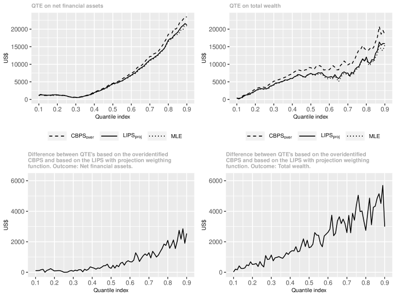
Figure 1: Estimated quantile treatment effects of 401(k) eligibility on different wealth measures.

The results in Panel A suggest that 401(k) eligibility has a positive and significant average impact on both net financial assets and total wealth and that the effect is more pronounced at the higher quantiles. When one compares the treatment effect measures across different PS estimation methods, we see that the results tend to be similar for net financial assets; for total wealth, we note that estimators based on the overidentified CBPS estimator suggest much larger effects of 401(k) eligibility at higher quantiles than those based on our proposed IPS estimators; see Figure 1 for a more detailed comparison between the QTE estimates based on the IPS with projection weighting function, overidentified CBPS (the default in the CBPS R package), and those based on ML.

The results in Panel B paint a similar picture as those in Panel A: 401(k) participation tends to have a positive and significant average impact on both measures of wealth, and the effect is more pronounced at the right tail of the wealth measures. As we illustrated in Figure 2, there are quantitative differences between the LQTE estimates based on different PS estimation methods, with those based on the overidentified instrument CBPS suggesting much larger effects than the other estimation methods, though the shape of the LQTE function is similar across specifications.

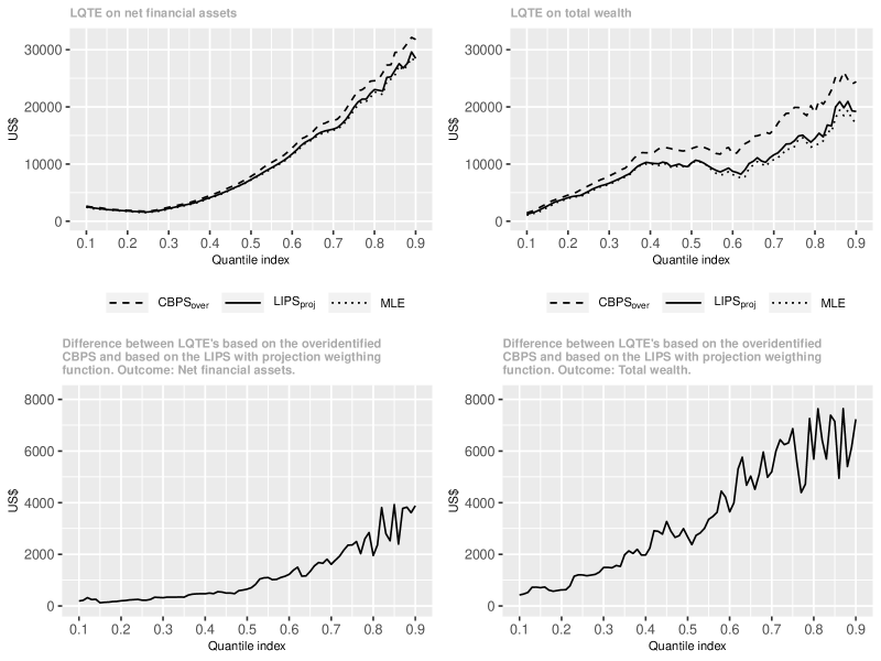
Figure 2: Estimated local quantile treatment effects of 401(k) participation on different wealth measures.

7 Conclusion

In this article, we proposed a framework to estimate propensity score parameters such that, instead of targeting to balance only some specific moments of covariates, it aims to balance all functions of covariates. The proposed estimator is of the minimum distance type, and is data-driven, $\sqrt{n}$-consistent, asymptotically normal, and admits an asymptotic linear representation that facilitates the study of inverse probability weighted estimators in a unified manner. Importantly, we have shown that our framework can accommodate the empirically relevant situation under which treatment allocation is endogenous. We derived the large sample properties of average, distributional and quantile treatment effect estimator based on the proposed integrated propensity scores, and illustrated its attractive properties via a Monte Carlo study and two empirical applications.

Although this paper devoted most of its attention to forming IPW-type treatment effect estimators, we note that sometimes researchers are willing to consider an outcome regression model, on top of the propensity score model. In such cases, we stress that one can easily combine our IPS estimation procedure with such outcome regression model to form doubly-robust, locally efficient treatment effect estimators, see, e.g., Sloczynski2018 and references therein. Perhaps even better, one can use the integrated moment approach adopted in this paper to estimate not only the propensity score, but also the outcome regression model. We leave the detailed discussion of such procedure for future research.

References

- (1)
- Abadie (2003) Abadie, A. (2003), “Semiparametric instrumental variable estimation of treatment response models,” Journal of Econometrics, 113, 231–263.
- Abadie et al. (2002) Abadie, A., Angrist, J. D., and Imbens, G. W. (2002), “Instrumental variables estimates of the effect of subsidized training on the quantiles of trainee earnings,” Econometrica, 70(1), 91–117.
- Ai and Chen (2003) Ai, C., and Chen, X. (2003), “Efficient estimation of models with conditional moment restrictions containin unknown functions,” Econometrica, 71(6), 1795–1843.
- Angrist et al. (1996) Angrist, J. D., Imbens, G. W., and Rubin, D. B. (1996), “Identification of causal effects using instrumental variables,” Journal of the American Statistical Association, 91(434), 444–455.
- Benjamin (2003) Benjamin, D. J. (2003), “Does 401(k) eligibility increase saving? Evidence from propensity score subclassification,” Journal of Public Economics, 87(5-6), 1259–1290.
- Bierens (1982) Bierens, H. J. (1982), “Consistent model specification tests,” Journal of Econometrics, 20(1982), 105–134.
- Bitler et al. (2006) Bitler, M. O., Gelbach, J. B., and Hoynes, H. H. (2006), “What mean impacts miss: Distributional effects of welfare reform experiments,” The American Economic Review, 96(4), 988–1012.
- Busso et al. (2014) Busso, M., Dinardo, J., and McCrary, J. (2014), “New Evidence on the Finite Sample Properties of Propensity Score Reweighting and Matching Estimators,” The Review of Economics and Statistics, 96(5), 885–895.
- Chen et al. (2008) Chen, X., Hong, H., and Tarozzi, A. (2008), “Semiparametric efficiency in GMM models with auxiliary data,” The Annals of Statistics, 36(2), 808–843.
- Chernozhukov et al. (2010) Chernozhukov, V., Fernández-Val, I., and Galichon, A. (2010), “Quantile and Probability Curves Without Crossing,” Econometrica, 78(3), 1093–1125.
- Chernozhukov et al. (2019) Chernozhukov, V., Fernández-Val, I., Melly, B., and Wüthrich, K. (2019), “Generic Inference on Quantile and Quantile Effect Functions for Discrete Outcomes,” Journal of the American Statistical Association, pp. 1–24.
- Chernozhukov and Hansen (2004) Chernozhukov, V., and Hansen, C. (2004), “The impact of 401(k) participation on the wealth distribution: an instrumental quantile regression analysis,” The Review of Economics and Statistics, 86(3), 735–751.
- Dehejia and Wahba (2002) Dehejia, R., and Wahba, S. (2002), “Propensity score-matching methods for nonexperimental causal studies,” The Review of Economics and Statistics, 84(1), 151–161.
- Díaz et al. (2015) Díaz, J., Rau, T., and Rivera, J. (2015), “A Matching Estimator Based on a Bilevel Optimization Problem,” Review of Economics and Statistics, 97(4), 803–812.
- DiNardo et al. (1996) DiNardo, J., Fortin, N. M., and Lemieux, T. (1996), “Labor Market Institutions and the Distribution of Wages , 1973-1992 : A Semiparametric Approach,” Econometrica, 64(5), 1001–1044.
- Dominguez and Lobato (2004) Dominguez, M. A., and Lobato, I. N. (2004), “Consistent Estimation of Models Defined by Conditional Moment Restrictions,” Econometrica, 72(5), 1601–1615.
- Domínguez and Lobato (2015) Domínguez, M. A., and Lobato, I. N. (2015), “A Simple Omnibus Overidentification Specification Test for Time Series Econometric Models,” Econometric Theory, 31(04), 891–910.
- Donald et al. (2003) Donald, S. G., Imbens, G. W., and Newey, W. K. (2003), “Empirical likelihood estimation and consistent tests with conditional moment restrictions,” Journal of Econometrics, 117(1), 55–93.
- Escanciano (2006a) Escanciano, J. C. (2006a), “A consistent diagnostic test for regression models using projections,” Econometric Theory, 22, 1030–1051.
- Escanciano (2006b) Escanciano, J. C. (2006b), “Goodness-of-Fit Tests for Linear and Nonlinear Time Series Models,” Journal of the American Statistical Association, 101(474), 531–541.
- Escanciano (2018) Escanciano, J. C. (2018), “A simple and robust estimator for linear regression models with strictly exogenous instruments,” Econometrics Journal, 21(1), 36–54.
- Fan et al. (2016) Fan, J., Imai, K., Liu, H., Ning, Y., and Yang, X. (2016), “Improving Covariate Balancing Propensity Score : A Doubly Robust and Efficient Approach,” Mimeo, pp. 1–47.
- Firpo (2007) Firpo, S. (2007), “Efficient semiparametric estimation of quantile treatment effects,” Econometrica, 75(1), 259–276.
- Firpo and Pinto (2016) Firpo, S., and Pinto, C. (2016), “Identification and Estimation of Distributional Impacts of Interventions Using Changes in Inequality Measures,” Journal of Applied Econometrics, 31(3), 457–486.
- Frölich (2007) Frölich, M. (2007), “Nonparametric IV estimation of local average treatment effects with covariates,” Journal of Econometrics, 139(1), 35–75.
- Frölich and Melly (2013) Frölich, M., and Melly, B. (2013), “Unconditional Quantile Treatment Effects Under Endogeneity,” Journal of Business & Economic Statistics, 31(3), 346–357.
- González-Manteiga and Crujeiras (2013) González-Manteiga, W., and Crujeiras, R. M. (2013), “An updated review of Goodness-of-Fit tests for regression models,” Test, 22(3), 361–411.
- Graham et al. (2012) Graham, B., Pinto, C., and Egel, D. (2012), “Inverse Probability Tilting for Moment Condition Models with Missing Data,” The Review of Economic Studies, 79(3), 1053–1079.
- Hainmueller (2012) Hainmueller, J. (2012), “Entropy balancing for causal effects: A multivariate reweighting method to produce balanced samples in observational studies,” Political Analysis, 20(1), 25–46.
- Hájek (1971) Hájek, J. (1971), “Discussion of ‘An essay on the logical foundations of survey sampling, Part I’, by D. Basu,” in Foundations of Statistical Inference, eds. V. P. Godambe, and D. A. Sprott, Toronto: Holt, Rinehart, and Winston.
- Heckman et al. (1997) Heckman, J. J., Ichimura, H., and Todd, P. (1997), “Matching as an econometric evaluation estimator: Evidence from evaluating a job training programme,” The Review of Economic Studies, 64(4), 605–654.
- Hellerstein and Imbens (1999) Hellerstein, J. K., and Imbens, G. W. (1999), “Imposing moment restrictions from auxiliary data by weighting,” Review of Economics and Statistics, 81(1), 1–14.
- Hirano et al. (2003) Hirano, K., Imbens, G. W., and Ridder, G. (2003), “Efficient estimation of average treatment effects using the estimated propensity score,” Econometrica, 71(4), 1161–1189.
- Ichino et al. (2008) Ichino, A., Mealli, F., and Nannicini, T. (2008), “From temporary help jobs to permanent employment: what can we learn from matching estimators and their sensitivity?,” Journal of Applied Econometrics, 23(3), 305–327.
- Imai and Ratkovic (2014) Imai, K., and Ratkovic, M. (2014), “Covariate balancing propensity score,” Journal of the Royal Statistical Society: Series B (Statistical Methodology), 76(1), 243–263.
- Imbens and Angrist (1994) Imbens, G. W., and Angrist, J. D. (1994), “Identification and estimation of local average treatment effects,” Econometrica, 62(2), 467–475.
- Imbens and Rubin (2015) Imbens, G. W., and Rubin, D. B. (2015), Causal Inference in Statistics, Social and Biometical Sciences, Cambridge, MA: Cambridge University Press.
- Kang and Schafer (2007) Kang, J. D. Y., and Schafer, J. L. (2007), “Demystifying Double Robustness: A Comparison of Alternative Strategies for Estimating a Population Mean from Incomplete Data.,” Statistical Science, 22(4), 569–573.
- Kline (2011) Kline, P. (2011), “Oaxaca-Blinder as a reweighting estimator,” American Economic Review, 101(3), 532–537.
- Koenker and Bassett (1978) Koenker, R., and Bassett, G. (1978), “Regression Quantiles,” Econometrica, 46(1), 33–50.
- Leeb and Pötscher (2005) Leeb, H., and Pötscher, B. M. (2005), “Model selection and inference: Facts and fiction,” Econometric Theory, 21(1), 21–59.
- Millimet and Tchernis (2009) Millimet, D. L., and Tchernis, R. (2009), “On the Specification of Propensity Scores, With Applications to the Analysis of Trade Policies,” Journal of Business & Economic Statistics, 27(3), 397–415.
- Newey and McFadden (1994) Newey, W. K., and McFadden, D. (1994), “Large sample estimation and hypothesis testing,” in Handbook of Econometrics, Vol. 4, Amsterdam: North-Holland: Elsevier, chapter 36, pp. 2111–2245.
- Rosenbaum (1987) Rosenbaum, P. R. (1987), “Model-Based Direct Adjustment,” Journal of the American Statistical Association, 82(398), 387–394.
- Rosenbaum and Rubin (1983) Rosenbaum, P. R., and Rubin, D. B. (1983), “The central role of the propensity score in observational studies for causal effects,” Biometrika, 70(1), 41–55.
- Rosenbaum and Rubin (1984) Rosenbaum, P. R., and Rubin, D. B. (1984), “Reducing bias in observational studies using subclassification on the propensity score,” Journal of the American Statistical Association, 79(387), 516–524.
- Rubin (2007) Rubin, D. B. (2007), “The design versus the analysis of observational studies for causal effects: Parallels with the design of randomized trials,” Statistics in Medicine, 26(1), 20–36.
- Rubin (2008) Rubin, D. B. (2008), “For objective causal inference, design trumps analysis,” Annals of Applied Statistics, 2(3), 808–840.
- Sant’Anna and Song (2019) Sant’Anna, P. H., and Song, X. (2019), “Specification tests for the propensity score,” Journal of Econometrics, 210(2), 379–404.
- Shaikh et al. (2009) Shaikh, A. M., Simonsen, M., Vytlacil, E. J., and Yildiz, N. (2009), “A specification test for the propensity score using its distribution conditional on participation,” Journal of Econometrics, 151(1), 33–46.
- Słoczyński and Wooldridge (2018) Słoczyński, T., and Wooldridge, J. M. (2018), “A General Double Robustness Result for Estimating Average Treatment Effects,” Econometric Theory, 34(1), 112–133.
- Stute (1997) Stute, W. (1997), “Nonparametric model checks for regression,” The Annals of Statistics, 25(2), 613–641.
- van der Vaart (1998) van der Vaart, A. W. (1998), Asymptotic Statistics, Cambridge: Cambridge University Press.
- Wüthrich (2019) Wüthrich, K. (2019), “A closed-form estimator for quantile treatment effects with endogeneity,” Journal of Econometrics, 210(2), 219–235.
- Zhao (2019) Zhao, Q. (2019), “Covariate balancing propensity score by tailored loss functions,” The Annals of Statistics, 47(2), 965–993.
- Zubizarreta (2015) Zubizarreta, J. R. (2015), “Stable Weights that Balance Covariates for Estimation With Incomplete Outcome Data,” Journal of the American Statistical Association, 110(511), 910–922.