A Comparative Study of Neural Network Models for Sentence Classification

Abstract

This paper presents an extensive comparative study of four neural network models, including feed-forward networks, convolutional networks, recurrent networks and long short-term memory networks, on two sentence classification datasets of English and Vietnamese text. We show that on the English dataset, the convolutional network models without any feature engineering outperform some competitive sentence classifiers with rich hand-crafted linguistic features. We demonstrate that the GloVe word embeddings are consistently better than both Skip-gram word embeddings and word count vectors. We also show the superiority of convolutional neural network models on a Vietnamese newspaper sentence dataset over strong baseline models. Our experimental results suggest some good practices for applying neural network models in sentence classification.

I Introduction

Neural network models have provided a powerful learning method for use in many natural language problems recently. There are two major types of neural networks architectures that can be combined in two ways: feed-forward networks and recurrent networks. While convolutional feed-forward networks are able to extract local patterns, recurrent neural networks are able to capture long-range dependency in the data by abandoning the Markov assumption.

With the emerging interests of the community in deep learning, there are numerous works in sentence modeling and classification which apply neural network models. However, to our knowledge, there is not any attempt to compare these models empirically in sentence classification, especially in a multilingual setting. In this paper, we explore different model architectures systematically and demonstrate that the best performance is obtained by convolutional neural network models. We compare feed-forward neural network, recurrent neural networks, and convolutional neural networks on two datasets: the UIUC question classification dataset for English and a vnExpress sentence dataset for Vietnamese.

The main contributions of this paper are as follows. First, we show that the CNN models without any feature engineering can outperform some existing competitive question classifiers with rich hand-crafted linguistic features. Second, we find that the GloVe word vectors are consistently better than both of the Skip-gram word vectors and word count vectors when being used in neural network models. Third, we show the superiority of convolutional neural network models on a Vietnamese newspaper sentence dataset over strong feed-forward neural network models. Finally, these results can serve as a baseline for future research in these problems.

The remainder of this paper is structured as follows. In Section II, we briefly describe the neural network architectures in use, including feed-forward networks, convolutional networks, recurrent networks and its variant long short-term memory networks. Section III presents the experimental datasets and extensive evaluation results. Section IV discusses the results and related work. Finally, Section V concludes the paper.

II Neural Network Models

II-A Feed-Forward Neural Network

Feed-forward Neural Network (FNN) consists of multiple layers of nodes. Each layer is fully connected to the next layer in the network. Nodes in the input layer represent the input data. All other nodes map inputs to outputs by a linear combination of the inputs with the node’s weights $\mathbf{w}$ and bias $\mathbf{b}$ and applying an activation function. This can be written in matrix form for FNN with $\ell+1$ layers as follows:

$$y(\mathbf{x})=f_{\ell}(\cdots f_{2}(\mathbf{w}_{2}^{\top}f_{1}(\mathbf{w}_{1}^{\top}\mathbf{x}+b_{1})+b_{2})\cdots+b_{\ell}).$$

Nodes in intermediate layers use logistic function $f(z_{i})=1/{[1+\exp(-z_{i})]}$. Nodes in the output layer use softmax function $f(z_{i})={\exp(z_{i})}/{\sum_{k=1}^{K}\exp(z_{k})}.$ The number of nodes $K$ in the output layer corresponds to the number of classes. FNN employs backpropagation for learning the model. We use the logistic loss function for optimization and L-BFGS as an optimization routine.

II-B Convolutional Neural Network

Convolutional Neural Network (CNN) is a class of FNN which is designed to require minimal preprocessing. The network learn filters that in traditional algorithms were hand-engineered. This independence from prior knowledge and human effort in feature engineering is a major advantage of CNN.

We build our CNN upon that of  [1] which is originally proposed for sentence classification. Our CNN consists of six main layers: (1) a look-up tables to encode words in sentences by their embeddings, (2) a convolutional layer to recognize $w$-grams, (3) a non-linear layer with the rectifier activation function, (4) a max pooling layer to determine the most relevant features, (5) a fully connected layer with drop-out and (6) a logistic regression layer (a linear layer with a softmax at the end) to perform classification.

Let $\mathbf{s}=[w_{1},w_{2},\dots,w_{n}]$ be a sentence of length $n$, where $w_{i}$ is the $i$-th word of the sentence. Each word $w_{i}$ is represented by its word embedding $\mathbf{x}_{i}$ which is a row vector of $d$ dimensions. The sentence $\mathbf{s}$ can now be viewed as a tensor $\mathbf{X}=[\mathbf{x}_{1},\mathbf{x}_{2},\dots,\mathbf{x}_{n}]^{\top}$ of size $n\times d$. This matrix is fed into the convolutional layer to extract higher level features. Given a window size $w$, a filter is seen as a weight tensor $\mathbf{F}$ of size $o\times d\times w$, where $o$ is the output frame size of the filter. The core of this layer is obtained from the application of the convolutional operator on the two tensors $\mathbf{X}$ and $\mathbf{F}$. The output layer of the convolutional layer is precisely computed as

$$\mathbf{Y}_{ti}=\sum_{j=1}^{d}\sum_{k=1}^{w}\mathbf{F}_{ijk}*\mathbf{X}_{t-1+k,j}+b_{i},$$

for all $t=1,2,\dots,n-w+1,\forall i=1,2,\dots,o$, where $\mathbf{b}=[b_{1},b_{2},\dots,b_{o}]$ is the bias tensor of size $o$. Then a rectifier linear unit layer is applied element-wise on the output layer to produce score tensor.

The pooling is then applied to further aggregate the features generated from the previous layer. The popular aggregating function is $\max$ as it bears responsibility for identifying the most important features. More precisely, the max pooling layer produces $\mathbf{z}=[z_{1},z_{2},\dots,z_{o}]$, where $z_{i}=\max_{1\leq t\leq n-w+1}\mathbf{Y}_{ti}$. This feature vector is then fed into a fully connected layer of standard FNN. Following the previous work [1], we execute a dropout for regularization by randomly setting to zero a proportion $p$ of the output elements. Finally, this feature vector is fed into a logistic regression layer to perform classification.

II-C Recurrent Neural Network

Given an input sequence $[\mathbf{x}_{1},\mathbf{x}_{2},\dots,\mathbf{x}_{n}]$, a standard Recurrent Neural Network (RNN) computes the hidden vector sequence $[\mathbf{h}_{1},\mathbf{h}_{2},\dots,\mathbf{h}_{n}]$ and outputs vector sequence $[\mathbf{y}_{1},\mathbf{y}_{2},\dots,\mathbf{y}_{n}]$ by iterating the following equations from $t=1$ to $n$:

$$\mathbf{h}_{t} =\sigma\left(\mathbf{W}\mathbf{x}_{t}+\mathbf{U}\mathbf{h}_{t-1}+\mathbf{b}^{h}\right)$$

$$\mathbf{y}_{t} =\mathbf{V}\mathbf{h}_{t}+\mathbf{b}^{y}$$

where $\mathbf{W},\mathbf{U},\mathbf{V}$ denote weight matrices (e.g., $\mathbf{W}$ is the input-hidden weight matrix, $\mathbf{U}$ is the hidden-hidden weight matrix, and $\mathbf{V}$ is the hidden-output weight matrix); the $\mathbf{b}$ terms denote bias vectors; and $\sigma$ is the hidden layer function, which is usually an element-wise application of a sigmoid function.

This simple RNN formulation is sensitive to the ordering of tokens in the sequence. It was first proposed by Elman [2]. Since we are concerned with the classification problem instead of sequence modeling, the hidden vector at the last time step $\mathbf{h}_{n}$ is fed into a fully connected layer with dropout and then a logistic regression layer to perform classification.

II-D LSTM Network

In this model, we represent the word sequence of a sentence with a LSTM recurrent neural network [3]. The LSTM unit at the $t$-th word consists of a collection of multi-dimensional vectors, including an input gate $\mathbf{i}_{t}$, a forget gate $\mathbf{f}_{t}$, an output gate $\mathbf{o}_{t}$, a memory cell $\mathbf{c}_{t}$, and a hidden state $\mathbf{h}_{t}$. The unit takes as input a $d$-dimensional input vector $\mathbf{x}_{t}$, the previous hidden state $\mathbf{h}_{t-1}$, the previous memory cell $\mathbf{c}_{t-1}$, and calculates the new vectors using the following six equations:

$$\mathbf{i}_{t} =\sigma\left(\mathbf{W}^{i}\mathbf{x}_{t}+\mathbf{U}^{i}\mathbf{h}_{t-1}+\mathbf{b}^{i}\right)$$

$$\mathbf{f}_{t} =\sigma\left(\mathbf{W}^{f}\mathbf{x}_{t}+\mathbf{U}^{f}\mathbf{h}_{t-1}+\mathbf{b}^{f}\right)$$

$$\mathbf{o}_{t} =\sigma\left(\mathbf{W}^{o}\mathbf{x}_{t}+\mathbf{U}^{o}\mathbf{h}_{t-1}+\mathbf{b}^{o}\right)$$

$$\mathbf{u}_{t} =\tanh\left(\mathbf{W}^{u}\mathbf{x}_{t}+\mathbf{U}^{u}\mathbf{h}_{t-1}+\mathbf{b}^{u}\right)$$

$$\mathbf{c}_{t} =\mathbf{i}_{t}\cdot\mathbf{u}_{t}+\mathbf{f}_{t}\cdot\mathbf{c}_{t-1}$$

$$\mathbf{h}_{t} =\mathbf{o}_{t}\cdot\tanh(\mathbf{c}_{t}),$$

where $\sigma$ denotes the logistic function, the dot product denotes the element-wise multiplication of vectors, $\mathbf{W}$ and $\mathbf{U}$ are weight matrices and $\mathbf{b}$ are bias vectors. The LSTM unit at $t$-th word receives the corresponding word embedding as input vector $\mathbf{x}_{t}$.

III Experiments

III-A Datasets

We use two datasets in this study. The first one is the UIUC English question classification dataset. This corpus contains 5,952 manually labeled questions of 6 coarse-grained classes and 50 fine-grained classes [4]. Among them, 500 questions are reserved as the test set. Question classification is an important task of question analysis which detects the answer type of the question. It helps filter out a wide range of candidate answers and determine answer selection strategies. [5] We report fine-grained classification accuracy on 50 classes.

The second dataset is a corpus of 20,000 Vietnamese sentences extracted from the vnExpress online newspaper. Each sentence is labeled with one of five categories: “education”, “entertainment”, “devices”, “health” and “business”. This dataset is randomly split into a training set of 16,000 sentences (80%) and a test set of 4,000 sentences (20%).

III-B Word Embeddings

The first feature set includes all unigram features which are raw word tokens. When using neural networks (MLR, FNN, CNN), we transform word tokens into low-dimensional vectors. In our method, each input word token is transformed into a vector either by looking up pre-trained word embeddings or by word hashing with a fixed dimension.

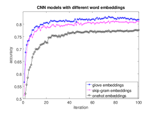
Figure 1: Accuracy of CNN models with different word embeddings, including 300-dimension GloVe vectors, 300-dimension Skip-gram vectors, and 1,024-dimension one-hot vectors. The maximal length of questions is fixed at 20 tokens.

For each word token of the input sentence of the UIUC data set, we map to its pre-trained 300-dimensional word vector, either being produced by the Skip-gram model trained on 3 billion running words of Google News corpus or by the GloVe model trained on 6 billion running words of Wikipedia 2014 and Gigaword corpus.. In the word hashing technique, each word token is mapped to an integer ranging from $0$ to $d$, where $d$ is the domain dimension. We use the hash function MurmurHash 3 as feature hashing technique, which is a fast and space-efficient way of vectorizing features.

Similarly, each word token of the Vietnamese sentence is mapped to its pre-trained 50-dimensional word vector. These word vectors are obtained by training a Skip-gram model on a Vietnamese text corpus of 7.3GB from 2 million articles collected through a Vietnamese news portal [6]. Note that each Vietnamese word may consist of more than one syllables with spaces in between, which could be regarded as multiple words by the unsupervised models. Hence it is necessary to replace the spaces within each word with underscores to create full word tokens.

In the following subsections, we first compare the performance of the models on the English UIUC corpus. We then compare the best CNN models on the Vietnamese corpus with baseline FNN models.

III-C CNN Results

In the first experiment, we study the effects of two word embeddings representations, either Skip-gram word vectors or GloVe word vectors, and the one-hot encoding representation with dimension $d=1,024$. The layer configuration of the CNNs are kept the same except the first embedding look-up tables. The convolutional layer has an output frame size of 256 and kernel width of 3. The non-linear layer has output size of 128 neurons. The dropout probability is fixed at $0.1$.

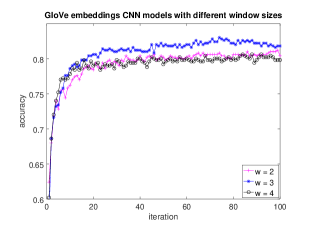
Figure 2: Accuracy of CNN models with different window sizes. The configuration of CNN models are kept the same except the window size $w$ is varied.

This experimental result is shown in Figure 1. The $x$-axis is the number of iterations in training the CNN models. The $y$-axis is accuracy ratio of the models on the test set. Among the three word representations, the GloVe representation gives the best result. It consistently outperforms the Skip-gram representation by a clear margin, achieves an accuracy of 83.00%; while the Skip-gram representation gives the maximal accuracy of 81.20%. The one-hot representation has the lowest accuracy, achieving 77.60%. This experimental result shows the good benefit of word embeddings learned from large unlabeled text data which capture syntactic and semantic information.

We also investigate the impact of window size $w$ to the accuracy of CNN models with GloVe embeddings. Figure 2 shows the test accuracy curves with three window sizes of 2, 3, and 4. It is clear that $w=3$ is the most appropriate window size which gives the best accuracy.

III-D RNN Results

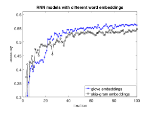
Figure 3: Accuracy of RNN models with two word embeddings schemes. The number of hidden units is fixed at 256. The GloVe embeddings outperform the Skip-gram embeddings.

In the second and third experiment, we investigate the performance of RNN and LSTM models respectively on the two word embedding schemes GloVe and Skip-gram under the same parameter settings.

We first evaluate the performance of RNN models. For each model, we tune the parameters by grid searching using the test set. The number of the hidden units in all models is fixed at 256, the batch size is 128, the learning rate is $10^{-2}$, the learning rate decay is $10^{-3}$, and the optimization algorithm is Adagrad. As in previous experiments, we set the iteration number over the training data as 100.

Figure 3 shows the accuracy curves of the two simple RNN models with the two embeddings schemes. The GloVe embeddings outperform the Skip-gram embeddings. The best accuracy of the two RNN models are 56.40% and 54.60% respectively.

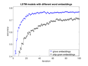
Figure 4: Accuracy of LSTM models with two word embeddings schemes. The number of hidden units is fixed at 256. The GloVe embeddings outperform significantly the Skip-gram embeddings.

Figure 4 shows the accuracy curves of the two LSTM models with either GloVe or Skip-gram embeddings. We see that the GloVe embeddings give significantly better result than the Skip-gram embeddings. After 100 training iterations, the best accuracy of the LSTM model with Skip-gram embeddings is only 71.60% while that of the LSTM model with GloVe embeddings is 76.80%. We also see that LSTM models outperform the simple RNN models by a clear margin but underperform CNN models. This experimental result demonstrates that CNN models are better than RNN models in capturing salient features.

III-E FNN Results

In the fourth experiment, we report the performance of FNN models using count vector representations. The count vector of a sentence is the common bag-of-word representation of its unigrams with a minimum frequency cutoff of 2 on the training set. In this representation, each input sentence is transformed into a count vector of size $d$, where $d$ is a fixed domain dimension used in the feature hashing technique. The FNN models use the same number of 256 units in the hidden layer as in the CNN and RNN experiments.

Figure 5: Accuracy of FNN models with one hidden layer of 256 units on the UIUC corpus. The $x$-axis shows the count vector encodings with different dimensions, ranging from 1,024 to 8,196.

Figure 5 shows the accuracy of FNN models. We see that these models fall behind CNN and RNN models with a large margin.

Table I: Accuracy scores of CNN, RNN and FNN models on the English UIUC question types dataset

Model	Accuracy
CNN with GloVe embeddings	83.00%
CNN with Skip-gram embedding	81.20%
CNN with one-hot embeddings	77.60%
RNN with GloVe embeddings	56.40%
RNN with Skip-gram embeddings	54.60%
LSTM with GloVe embeddings	76.80%
LSTM with Skip-gram embeddings	71.60%
FNN with bag-of-word vectors	76.00%

Table I summarizes the best accuracy scores of the models. The CNN models are better than the other models by a large margin. The best model is CNN with GloVe embeddings.

III-F vnExpress Results

In this subsection, we compare the performance of neural networks models on the vnExpress corpus. In the fifth experiment, we report experimental results of the CNN models with different feature encodings, as shown in the Figure 6. We see that the word embeddings encoding is slightly outperformed by bag-of-word encodings with large domain dimensions. However, the training time of the model with the $8,192$-dimensional bag-of-word encoding is about four times slower than that of the Skip-gram embeddings.

Figure 6: Accuracy of CNN models on the vnExpress corpus. The $x$-axis shows the bag-of-word encodings with different dimensions, ranging from 1,024 to 8,196 and the Skip-gram word embeddings of 50 dimensions.

Finally, in the sixth experiment, we report the accuracy of the FNN models on the Vietnamese dataset. In both of the CNN and the FNN models, we do not tune them for their best performance but intentionally use a fully-connected hidden layer of the same 256 hidden units. With this setting, their salient feature detection capability can be directly comparable. Figure 7 shows the result. We see that the best FNN model is worse than all CNN models: the accuracy gap between the two best models is about 6% of absolute points.

Figure 7: Accuracy of FNN models with one hidden layer of 256 units on the vnExpress corpus. The $x$-axis shows the bag-of-word encodings with different dimensions, ranging from 1,024 to 8,196.

IV Discussion

RNN models have been shown to be a very strong sequence learner in that it can detect intricate patterns in the data and long-range dependency. However, we show that this power is not needed for sentence classification in both the UIUC question dataset for English and the vnExpress sentence dataset for Vietnamese. The word order and sentence structure are not really important in these cases. The bag-of-word or bag-of-ngram classifier just work as well or even better than RNN models, including the powerful LSTM models.

The CNN models for sequence learner have been designed to identify indicative local features in a long sequence and to combine them. They are able to capture $n$-grams that are predictive for sentence classification, without the need to specify a very sparse vector for each possible $n$-gram as in the traditional bag-of-ngram approach. As a result, CNN models are not only effective – avoiding data sparsity problems, but also scalable – any window size produces a fixed size vector representation of the sentence. Our experiments have demonstrated that CNN models outperform all other strong competitive models on two sentence datasets of different natural languages.

In our experiments, we do not use any feature engineering, only raw sentences are provided. All the models only use either word identity or pre-trained word embeddings for the concerned languages (300-dimensional Skip-gram word vectors, 300-dimensional GloVe word vectors for English, and 50-dimensional Skip-gram word vectors for Vietnamese). The models can be thus considered language-independent.

In particular, on the UIUC question dataset, Li and Roth [4] developed the first machine learning approach to question classification which uses the SNoW learning architecture. Using the feature set of lexical words, part-of-speech tags, chunks and named entities, they achieved 78.8% of fine-grained accuracy. The UIUC dataset has inspired many follow-up works on question classification. Zhang and Lee [7] used linear support vector machines (SVM) with all question $n$-grams and obtained 79.2% of accuracy. Hacioglu and Ward [8] used linear SVM with question bigrams and error-correcting codes and achieved 82.0% of accuracy. Our CNN models with GloVe embeddings can achieve 83.00% of fine-grained accuracy, which are better than some early question classifiers.

V Conclusion

In this paper, we compare different neural network models for sentence classification, including FNN, RNN, LSTM, and CNN networks. In these models, features are automatically learned without any complicated natural language processing. Experimental results on two sentence datasets, one for English and one for Vietnamese show that the CNN models significantly outperform other models on both of the datasets. In particular, on the UIUC English question classification dataset, the GloVe embeddings are consistently better than the Skip-gram embeddings. On this dataset, our CNN models without any feature engineering also outperform some existing question classifiers with rich hand-crafted linguistic features.

References

- [1] Y. Kim, “Convolutional neural networks for sentence classification,” in Proceedings of EMNLP. Doha, Quatar: ACL, 2014, pp. 1746–1751.
- [2] J. L. Elman, “Finding structure in time,” Cognitive Science, vol. 14, no. 2, pp. 179–211, 1990.
- [3] A. Graves, A.-R. Mohamed, and G. Hinton, “Speech recognition with deep recurrent neural networks,” in Proceedings of IEEE ICASSP. IEEE, 2013, pp. 6645–6649.
- [4] X. Li and D. Roth, “Learning question classifiers,” in Proceedings of COLING, 2002, pp. 556–569.
- [5] P. Le-Hong, P. Xuan-Hieu, and N. Tien-Dung, “Using dependency analysis to improve question classification,” in Knowledge and Systems Engineering. Springer, 2014, vol. 326, pp. 653–665.
- [6] P. Le-Hong, T.-M.-H. Nguyen, T.-L. Nguyen, and M.-L. Ha, “Fast dependency parsing using distributed word representations,” in Trends and Applications in Knowledge Discovery and Data Mining, ser. LNAI. Springer, 2015, vol. 9441.
- [7] D. Zhang and W. S. Lee, “Question classification using support vector machines,” in Proceedings of the 26th ACM SIGIR, 2003, pp. 26–32.
- [8] K. Hacioglu and W. Ward, “Question classification with support vector machines and error correcting codes,” in Proceedings of NAACL/HLT, 2003, pp. 28–30.
- [9] X. Li and D. Roth, “Learning question classifiers: the role of semantic information,” Natural Language Engineering, vol. 12, no. 3, pp. 229–249, 2006.
- [10] N. L. Minh, N. T. Thanh, and S. Akira, “Subtree mining for question classification problem,” in Proceedings of IJCAI, 2007, pp. 1695–1700.
- [11] Z. Huang, M. Thint, and Z. Qin, “Question classification using head words and their hypernyms,” in Proceedings of the 2008 Conference on EMNLP, 2008, pp. 927–936.
- [12] N. Van-Tu and L. Anh-Cuong, “Improving question classification by feature extraction and selection,” Indian Journal of Science and Technology, vol. 9, no. 17, 2016.
- [13] D. H. Tran, C. X. Chu, S. B. Pham, and M. L. Nguyen, “Learning based approaches for vietnamese question classification using keywords extraction from the web,” in Proceedings of IJCNLP, Nagoya, Japan, 2013, pp. 740–746.