Physical properties of the fullerene C₆₀-containing planetary nebula SaSt 2-3

Abstract

We perform a detailed analysis of the fullerene C₆₀-containing planetary nebula (PN) SaSt 2-3 to investigate the physical properties of the central star (B0-1II) and nebula based on our own Subaru/HDS spectra and multiwavelength archival data. By assessing the stellar absorption, we derive the effective temperature, surface gravity, and photospheric abundances. For the first time, we report time variability of the central star’s radial velocity, strongly indicating a binary central star. Comparison between the derived elemental abundances and those predicted values by asymptotic giant branch (AGB) star nucleosynthesis models indicates that the progenitor is a star with initial mass of $\sim$1.25 M_☉ and metallicity $Z=0.001$/$\alpha$-element/Cl-rich ([$\alpha$,Cl/Fe]$\sim$+0.3-0.4). We determine the distance (11.33 kpc) to be consistent with the post-AGB evolution of 1.25 M_☉ initial mass stars with $Z=0.001$. Using the photoionisation model, we fully reproduce the derived quantities by adopting a cylindrically shaped nebula. We derive the mass fraction of the C-atoms present in atomic gas, graphite grain, and C₆₀. The highest mass fraction of C₆₀ ($\sim$0.19 %) indicates that SaSt 2-3 is the C₆₀-richest PN amongst Galactic PNe. From comparison of stellar/nebular properties with other C₆₀ PNe, we conclude that the C₆₀ formation depends on the central star’s properties and its surrounding environment (e.g., binary disc), rather than the amount of C-atoms produced during the AGB phase.

1 Introduction

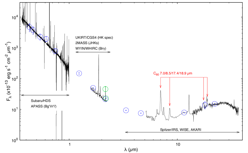
Figure 1: Panchromatic data of SaSt 2-3 used in the present work. The green (WHIRC Br$\gamma$-on/off bands) and blue circles (the other bands) are the photometry data and the black lines are the spectra, respectively. The flux density of the Subaru/HDS spectrum is scaled to match the APASS $Bg^{\prime}Vr^{\prime}i^{\prime}$-bands. The UKIRT 3.8 m/Cooled Grating Spectrometer 4 (CGS4) $HK$-band spectrum (we downloaded the raw data of the spectrum presented in Lumsden et al. (2001) from the UKIRT archive data website and reduced them using IRAF) is scaled to match the 2MASS $Ks$-band. The Spitzer/IRS spectrum is scaled to match the WISE/W3 and W4 and AKARI L18W bands.

Mid-infrared (mid-IR) spectroscopic observations made by the Spitzer/Infrared Spectrograph (IRS, Houck et al., 2004) have recently detected fullerene C₆₀ and C₇₀ in a variety of space environments such as R Coronae Borealis stars (García-Hernández et al., 2011a), reflection nebulae (Sellgren et al., 2010), young stellar objects (Roberts et al., 2012), post asymptotic giant branch (AGB) stars (Gielen et al., 2011a; Gielen et al., 2011b), proto planetary nebula (PNe; Zhang & Kwok, 2011), and PN (Cami et al., 2010; García-Hernández et al., 2010, 2011b, 2012; Otsuka et al., 2013, 2014; Otsuka et al., 2016). At the moment, PNe represent the largest fraction of fullerene detection; since the first detection of the mid-IR C₆₀ and C₇₀ bands in the C-rich PN Tc 1 by Cami et al. (2010), 24 fullerene-containing PNe have been identified in the Milky Way and the Large and Small Magellanic Clouds (LMC and SMC, respectively).

In general, C₆₀ PNe show very similar IR dust features and stellar/nebular properties; their mid-IR spectra display broad $6-9$, 11, and 30 µm features in addition to C₆₀ bands at 7.0, 8.5, 17.4, and 18.9 µm, and they have cool central stars and low-excitation nebulae, indicating that their age after the AGB phase is very young (e.g., Otsuka et al., 2014). The excitation mechanisms (e.g., Bernard-Salas et al., 2012) and the formation paths (e.g., Berné et al., 2015; Duley & Hu, 2012) are not well understood and are still a subject of debate. However, it remains unclear why these objects exhibit the C₆₀ features - is the span of time during which spectral features of C₆₀ are present a short-lived phase that all C-rich PNe go through, or are C₆₀ PNe distinct objects in terms of their stellar/nebular properties and/or evolution? This is directly linked to the question of how C₆₀ forms in evolved star environments. We would like to answer this fundamental question by investigating the physical properties of C₆₀ PNe and comparing them with non-C₆₀ PNe.

Amongst C₆₀ PNe, SaSt 2-3 (PN G232.0+05.7, Acker et al., 1992) firstly identified by Sanduleak & Stephenson (1972) is a particularly interesting object to that we should pay more attention. Otsuka et al. (2014) discovered C₆₀ bands in this PN for the first time. Surprisingly, the mid-IR C₆₀ band strengths in SaSt 2-3 and Tc 1 are the strongest amongst all the fullerene-containing objects. This strongly indicates that the fullerene formation in these two PNe is particularly efficient. Tc 1 has been extensively studied since the discovery of C₆₀. However, SaSt 2-3 is not entirely understood due to the lack of available data for the central star and nebula and its uncertain distance ($D$). The uncertain $D$ towards SaSt 2-3 has led to different estimates of the central star luminosity ($L_{\ast}$) and effective temperature ($T_{\rm eff}$); accordingly, this has led to inconsistencies in understanding the evolutionary status of this PN (Gesicki & Zijlstra, 2007; Otsuka et al., 2014). What we know from the prior studies is that this object has low-metallicity ($\epsilon({\rm S})$ = 5.48, Pereira & Miranda, 2007) and is (possibly) a Type IV PN (i.e, halo population, Pereira & Miranda, 2007).

If we obtain the UV to optical wavelength spectra of the central star as well as the nebula, we can resolve issues raised and verify conclusions from previous studies of SaSt 2-3; by so doing, we can hope to gain insights into the C₆₀ formation. Fortunately, the UV-optical photometry data from the AAVSO Photometric All Sky Survey (APASS, Henden et al., 2016) can rigorously constrain $L_{\ast}$, and Frew et al. (2016) improved its distance estimate ($D=14.86~{}\pm~{}4.26$ kpc). Therefore, we perform a comprehensive analysis on our own high-dispersion spectra of SaSt 2-3 taken using the 8.2 m Subaru telescope/high dispersion spectrograph (HDS, Noguchi et al., 2002) and archived multiwavelength data.

We organise the next sections as follows. In § 2, we describe our HDS spectroscopy and near-IR imaging using the NOAO WIYN 3.5 m/WIYN High-Resolution Infrared Camera (WHIRC, Meixner et al., 2010) and the reduction of this data. The Spitzer/IRS observation and its data reduction are described in Otsuka et al. (2014). In Fig. 1, we plot all the data used in the present work. In § 3, we perform plasma-diagnostics and derive ionic/elemental abundances. In § 4, we derive photospheric elemental abundances, $T_{\rm eff}$, and surface gravity $\log\,g$ by fitting the stellar absorption using the theoretical stellar atmosphere code TLUSTY (Hubeny, 1988). In § 5, we compare the derived nebular and stellar elemental abundances with those values predicted by AGB nucleosynthesis models in order to infer the initial mass of the progenitor star. In § 6, we build the spectral energy distribution (SED) model using the photoionisation code Cloudy (v.13.05, Ferland et al., 2013) to be consistent with all the derived quantities based on our determined $D$. In § 7, we discuss the origin and evolution of SaSt 2-3 and the C₆₀ formation in PNe by comparison of the derived nebular/stellar properties with other non-C₆₀ and C₆₀-containing PNe. Finally, we summarise the present work.

2 Data Set and Reduction

2.1 Subaru/HDS observation

We secured high-dispersion echelle spectra using the HDS located at one of the Nasmyth loci of the 8.2 m Subaru Telescope at the top of Mauna Kea in Hawai’i. We summarise our observations in Table 1. We selected the $2\times 2$ on-chip binning pattern. We set the slit-width to be 1.2″. We used the blue cross disperser for the $3640-5390$ Å observation and the red one for the $4740-7490$ Å and $7190-9960$ Å observations, respectively. We utilised the atmospheric dispersion corrector (ADC) during the observations. In all the observations, we observed the standard star Hiltner 600 for correcting echelle blaze functions and flux density simultaneously. In the $7190-9960$ Å observation, we observed the telluric standard stars HD 61017 (B9III, $m_{\rm V}=6.68$) and HD 62217 (B9V, $m_{\rm V}=8.26$) at similar airmass.

We reduced the data using IRAF in a standard manner, including over-scan subtraction, scattered light subtraction between echelle orders, and telluric absorption removal. We adopted the atmospheric extinction correction function measured by Buton et al. (2013) at Mauna Kea. We measured the actual spectral resolution ($R=\lambda/\delta{\lambda}=32\,300-33\,500$, see Table 1) using $>$300 Th-Ar comparison lines. The signal-to-noise ratio (S/N) for continuum reaches $\sim$40 at $\sim$3640 Å and $\sim$11 at $\sim$9950 Å. In $\sim$$3700-4800$ Å (this range is important in stellar absorption fittings), S/N is $>$70. We scaled both spectra to the average flux density in the overlapping regions ($4740-5390$ Å and $7190-7490$ Å), and we connected these scaled spectra into a single $3640-9960$ Å spectrum. The resultant spectrum is presented in Fig. 1.

2.2 Flux measurements and interstellar extinction correction

We measure emission line fluxes by multiple Gaussian component fitting. Then, we correct these observed fluxes $F$($\lambda$) to obtain the interstellar extinction corrected fluxes $I$($\lambda$) using the following formula;

$$I(\lambda)=F(\lambda)~{}\cdot~{}10^{c({\rm H\beta})(1+f(\lambda))},$$ (1)

where $f$($\lambda$) is the interstellar extinction function at $\lambda$ computed by the reddening law of Cardelli et al. (1989). To verify $R_{V}$ accurately, $\sim$$2000-2500$ Å spectra/photometry data would be necessary because $f({\lambda})$ and $R_{V}$ are sensitive to this wavelength range. At the moment, there are no available spectra/photometry data in such wavelength range. Therefore, we adopt an average $R_{V}=3.1$ in the Milky Way. Applying $R_{V}=3.1$ to SaSt 2-3 seems to be acceptable because Wegner (2003) reported $R_{V}=3.64~{}\pm~{}0.43$ towards HD 60855 (B2Ve). HD 60855 is a star in the direction closer to SaSt 2-3 amongst stars whose $R_{V}$ has been measured. $c$(H$\beta$) is the reddening coefficient at H$\beta$, corresponding to $\log_{10}$ $I$(H$\beta$)/$F$(H$\beta$).

We determine $c$(H$\beta$) values by comparing the observed Balmer and Paschen line ratios to H$\beta$ with the theoretical ratios of Storey & Hummer (1995) for the case with an electron temperature $T_{\rm e}$ = 10⁴ K and an electron density $n_{\rm e}$ = 2000 cm^-3 under the Case B assumption. We calculate this $n_{\rm e}$ using the [O ii] $F$(3726 Å)/$F$(3729 Å) and the [Cl iii] $F$(5517 Å)/$F$(5537 Å) ratios. For the $3640-5390$ Å spectrum, we obtain $c$(H$\beta$) = $0.20~{}\pm~{}0.01$, which is the intensity-weight average amongst the H$\gamma$, H$\delta$, H$\epsilon$, and H$\eta$ to the H$\beta$ ratios. For the $4740-7490$ Å spectrum, we obtain $c$(H$\beta$) = $0.40~{}\pm~{}0.01$ from the H$\alpha$/H$\beta$ ratio. For the $7190-9960$ Å spectrum, we determine $c$(H$\beta$) = $0.24~{}\pm~{}0.03$ from the Paschen H i 9014 Å (P10) to the H$\beta$ ratio. For all HDS spectra, we adopt the average $c$(H$\beta$) = $0.28~{}\pm~{}0.11$ amongst three HDS observations.

Tylenda et al. (1992) reported $c$(H$\beta$) = 1.11 (observation date is unknown). We derive the average $c$(H$\beta$) = $1.11~{}\pm~{}0.26$ using the ratio of $F$(H$\alpha$), $F$(H$\gamma$), and $F$(H$\delta$) to $F$(H$\beta$) measured from their spectrum. Based on the $F$(H$\alpha$) and $F$(H$\beta$) reported by Dopita & Hua (1997), we obtain $c$(H$\beta$) = $0.43~{}\pm~{}0.04$ (obs date: 1997 March). Pereira & Miranda (2007) reported $E(B-V)=0.11~{}\pm~{}0.02$, which corresponds to $c$(H$\beta$) = $0.13-0.19$ (obs date: 2005 Feb). Using the line flux table of Pereira & Miranda (2007), we obtain the average $c$(H$\beta$) = $0.41~{}\pm~{}0.23$ calculated from $F$(H$\alpha$), $F$(H$\gamma$), and $F$(P10) to $F$(H$\beta$). Using the archived ESO Faint Object Spectrograph and Camera (EFOSC) spectrum taken on 2000 April, we obtain a $c$(H$\beta$) = $0.68~{}\pm~{}0.11$ measured from the $F$(H$\alpha$)/$F$(H$\beta$) ratio. A time variation of $c$(H$\beta$) seen between 1992 and 2016 might be due to affect of stellar H i absorption to corresponding nebular H i and also orbital motion of the binary central star (§ 4.2).

We scale the Spitzer/IRS spectrum to match the Wide-field Infrared Survey Explorer (WISE) W3/W4 band flux densities of Cutri (2014) and the L18W AKARI/IRC mid-infrared all-sky survey of Ishihara et al. (2010) (see § 2.4). For this scaled Spitzer/IRS spectrum, we do not correct interstellar extinction because the interstellar extinction is negligibly small in the mid-IR wavelength. It is common practice in nebular analyses to scale all line intensities in such a way that H$\beta$ has a line flux of 100. To achieve this, we first normalise the line fluxes with respect the complex of the H i 7.46 µm ($n=5-6$, $n$ is the quantum number) and 7.50 µm ($n=6-8$) lines. $F$(7.48/7.50 µm) is $(4.87~{}\pm~{}0.30)\times 10^{-15}$ erg s^-1 cm^-2 ($A(-B)$ means $A\times 10^{-B}$ hereafter). According to Storey & Hummer (1995) for the Case B assumption with $T_{\rm e}$ = 10⁴ K and $n_{\rm e}$ = 2000 cm^-3, the ratio of H i $I$(7.48/7.50 µm)/$I$(H$\beta$) = 3.102/100. Finally, we multiply all the normalised line fluxes by 3.102 to express them relative to H$\beta$ with $I$(H$\beta$) = 100.

In Appendix Table A12, we list the identified emission lines in the Subaru/HDS and Spitzer/IRS spectra. The first column is the laboratory wavelength in air. Here, $I$(H$\beta$) is 100. The last column $\delta$ $I(\lambda)$ corresponds to 1-$\sigma$.

Table 1: HDS and WHIRC observation log for SaSt 2-3.

Date	$\lambda$ (Å)	$\lambda/\delta\,\lambda$ (ave.)	Exp. time	Condition/Seeing
2013/10/06	$3640-5390$	33 500	$2\times 200$ s, 2600 s	thin cloud, $\sim$0.7″
2013/12/10	$4740-7490$	33 300	100, 500, 900 s	clear, $\sim$0.7″
2016/02/01	$7190-9960$	32 300	180 s, $4\times 1600$ s	clear, $\sim$0.7-1.0″
Date	Band	Pixel scale	Exp. time	Condition/Seeing
2013/04/24	Br$\gamma$, Br$\gamma$45	0.1″$\times$0.1″	5 pts $\times$ 120 s	clear,$\sim$0.6-0.7″

2.3 NOAO/WHIRC near-IR imaging observation

We took the high-resolution images using NOAO WIYN 3.5 m/WHIRC. We summarise the observation log in Table 1. We took the two narrowband images using the Br$\gamma$ ($\lambda_{\rm c}=2.162$ µm, effective band width ($W_{\rm eff}$) = 0.210 µm) and Br$\gamma$45 ($\lambda_{\rm c}=2.188$ µm, $W_{\rm eff}=0.245$ µm) filters. We selected a 5 pts dithering pattern. We followed a standard manner for near-IR imaging data reductions using IRAF, including background sky and dark current subtraction, bad pixel masking, flat-fielding, and distortion correction. Finally, we obtained a single averaged image for each band.

For the flux calibration, we utilised the SED of the standard star 2MASS07480394-1407155 based on its photometry between the two micron all sky survey (2MASS, Cutri et al., 2003) $JHKs$ and WISE bands W1/W2. The SED of this star can be well fitted with a single blackbody temperature of 3510 K. Then, we derived the flux density in each band by taking each filter transmission curve into account. Next, we measured the respective count of the standard star in the Br$\gamma$ and Br$\gamma$45 images. Thus, we obtained the conversion factor from the counts in ADU to flux density in erg s^-1 cm^-2 µm^-1. The measured flux density in each band is listed in Appendix Table A2 and plotted in Fig. 1 (green circles).

2.4 Photometry data

To support the present work, we collected the data taken from APASS, 2MASS, WISE, and AKARI/Infrared Camera (IRC). In Table A2, we list the observed and reddening corrected flux densities $F_{\lambda}$ and $I_{\lambda}$, respectively. We obtain $I_{\lambda}$ using Equation (1) and the average $c$(H$\beta$) = $0.28~{}\pm~{}0.11$ amongst three HDS observations (§ 2.2). Due to negligibly small reddening effect, we do not correct $F_{\lambda}$ in the longer wavelength than WISE W1 band (3.35 µm).

3 Nebular line analysis

3.1 Systemic nebular radial velocity

We obtain the average heliocentric radial velocity of +166.6 km s^-1 measured from the identified 128 nebular lines in the HDS spectrum (the standard deviation is 3.2 km s^-1 amongst all these lines and that of each radial velocity is 0.52 km s^-1 in the average). The LSR radial velocity $v_{r}$(LSR) of +149.1 km s^-1 is much faster than $v_{r}$(LSR) in other Galactic PNe toward $l$ $\sim$$220-240$^∘ and $b\lesssim\pm$10^∘ ($\lesssim+80$ km s^-1; Quireza et al., 2007). $v_{r}$(LSR) of +105 km s^-1 in the C₆₀ PN M1-9 (PN G214.0+04.3, Otsuka et al., 2014) is the closest to SaSt 2-3’s $v_{r}$(LSR) (Quireza et al., 2007). Peculiar velocity relative to Galactic rotation is calculated using $v_{r}$(LSR) and $D$ in order to classify PNe into Type I-IV (i.e., thin/thick disc and halo; see e.g., Peimbert, 1978). We discuss classification of SaSt 2-3 in § 7.1. We do not find a time-variation of the radial velocity measured by the nebular lines. We report the radial velocity measurements from the stellar absorption in § 4.2.

3.2 H$\beta$ flux of the entire nebula

From the measured $F$(H i 7.48/7.50 µm) and the theoretical $I$(H i 7.48/7.50 µm)/$I$(H$\beta$) ratio = 3.102/100 (see § 2.2), we obtain $I$(H$\beta$) of the entire nebula to be $(1.57~{}\pm~{}0.28)(-12)$ erg s^-1 cm^-2. $F$(H$\alpha$) and $F$(H$\beta$) using the 5″ wide slit observation by Dopita & Hua (1997) and $c$(H$\beta$) = $0.43~{}\pm~{}0.04$ (§ 2.2) yields $I$(H$\beta$) = $(1.97~{}\pm~{}0.20)(-12)$ erg s^-1 cm^-2, which is consistent with ours. In the present work, we adopt our own calculated $I$(H$\beta$) for the entire nebula because our $I$(H$\beta$) is based on interstellar extinction free and stellar H i absorption effect less mid-IR H i 7.48/7.50 µm.

3.3 Plasma diagnostics

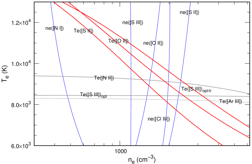
Figure 2: $n_{\rm e}-T_{\rm e}$ diagram of SaSt 2-3. $n_{\rm e}$, $T_{\rm e}$, and both $n_{\rm e}$ and $T_{\rm e}$ diagnostic curves are indicated by the blue, grey, and red lines, respectively. $T_{\rm e}$([S iii])_opt and $T_{\rm e}$([S iii])_opt/ir curves are the results by the [S iii] $I$(9069 Å)/$I$(6313 Å) and [S iii] $I$(9069 Å)/$I$(18.71/33.47 µm) ratios, respectively. See also Table 2.

Table 2: Summary of plasma diagnostics. Since the lower limit [N i] $I$(5198 Å)/$I$(5200 Å) ratio is out of the range of the $n_{\rm e}$([N i]) derivation, we give the upper limit $n_{\rm e}$($[$N i$]$) = 1460 cm^-3.

CEL $n_{\rm e}$-diagnostic line ratio	Ratio	Result (cm-3)
$[$N i$]$ $I$(5198 Å)/$I$(5200 Å)	$1.088~{}\pm~{}0.498$	$460$
[S ii] $I$(6717 Å)/$I$(6731 Å)	$0.663~{}\pm~{}0.074$	$2680~{}\pm~{}1070$
[O ii] $I$(3726 Å)/$I$(3729 Å)	$1.440~{}\pm~{}0.163$	$1560~{}\pm~{}490$
[Cl iii] $I$(5517 Å)/$I$(5537 Å)	$1.048~{}\pm~{}0.130$	$2180~{}\pm~{}1070$
[S iii] $I$(18.71 µm)/$I$(33.47 µm)	$1.314~{}\pm~{}0.334$	$1190~{}\pm~{}570$
CEL $T_{\rm e}$-diagnostic line ratio	Ratio	Result (K)
[N ii] $I$(6548/83 Å)/$I$(5755 Å)	$114.881~{}\pm~{}8.621$	$9200~{}\pm~{}260$
[S iii] $I$(9069 Å)/$I$(6313 Å)	$14.443~{}\pm~{}2.558$	$8530~{}\pm~{}570$
[Ar iii] $I$(7135/7751 Å)/$I$(8.99 µm)	$0.952~{}\pm~{}0.197$	$8250~{}\pm~{}790$
CEL $n_{\rm e}$ & $T_{\rm e}$-diagnostic line ratio	Ratio	Result (K)
[S ii] $I$(6717/31 Å)/$I$(4069 Å)	$10.322~{}\pm~{}0.958$	$7220~{}\pm~{}430$
[O ii] $I$(3726/3729 Å)/$I$(7320/30 Å)	$26.725~{}\pm~{}2.103$	$9670~{}\pm~{}430$
[S iii] $I$(9069 Å)/$I$(18.71/33.47 µm)	$0.278~{}\pm~{}0.054$	$11\,040~{}\pm~{}1860$
RL $T_{\rm e}$-diagnostic line ratio	Ratio	Result (K)
$[I_{\lambda}(8194\,{\AA})-I_{\lambda}(8169\,{\AA})]/I$(P11)	$0.022~{}\pm~{}0.004$	$7340~{}\pm~{}2610$
He i $I$(7281 Å)/$I$(6678 Å)	$0.256~{}\pm~{}0.036$	$11\,830~{}\pm~{}1790$

We determine $n_{\rm e}$ and $T_{\rm e}$ using diagnostic line ratios listed in Table 2, with the resulting $n_{\rm e}$-$T_{\rm e}$ diagnostic curves for the collisionally excited lines (CELs) shown in Fig. 2. The roughly vertical (blue) lines can be used to determine $n_{\rm e}$; more horizontal (grey) lines $T_{\rm e}$. Although the other diagnostic curves (red) yield both $n_{\rm e}$ and $T_{\rm e}$, we use them as $T_{\rm e}$ indicators here. Since the emission of each ion originates from regions of different $T_{\rm e}$ and $n_{\rm e}$, we need to determine both parameters for each ion independently so that we can determine accurate ionic abundances later on. This involves several steps. First, we note that $T_{\rm e}$ $\sim$9000 K from $T_{\rm e}$([Ar iii]), $T_{\rm e}$([S iii])_opt, and $T_{\rm e}$([N ii]) curves. Next, we adopt $T_{\rm e}$ = 9000 K to solve each equation of population at $\geq 5$ multiple energy levels for each $n_{\rm e}$ sensitive ions; from this, we then calculate $n_{\rm e}$ from the corresponding diagnostic line ratios for [N i], [S ii], [O ii], [Cl iii], and [S iii] (see Table 2). Note that the precise $T_{\rm e}$ we assume here does not matter much, since these $n_{\rm e}$ diagnostic line ratios are fairly insensitive to $T_{\rm e}$. With the $n_{\rm e}$ values established, we then determine $T_{\rm e}$ by adopting the derived $n_{\rm e}$ values corresponding to each ion. We adopt $n_{\rm e}$([O ii]) for $T_{\rm e}$([N ii]) derivation. Our derived values are in agreement with those by Pereira & Miranda (2007) who found $n_{\rm e}$([S ii]) = $2100~{}\pm~{}600$ cm^-3 and $T_{\rm e}$([N ii]) = $9600~{}\pm~{}930$ K.

We compute $T_{\rm e}$(He i) using singlet He i lines. To calculate $T_{\rm e}$(PJ) from the Paschen continuum discontinuity by utilising the equation (7) of Fang & Liu (2011), first we determine the He⁺ abundance of $1.09(-2)~{}\pm~{}2.28(-4)$ under the obtained $T_{\rm e}$(He i). Eventually, we utilise $T_{\rm e}$(He i) for both He⁺ and C²⁺ abundance calculations due to higher $T_{\rm e}$(PJ) uncertainty.

3.4 Ionic abundance derivations

Table 3: Adopting $T_{\rm e}$ and $n_{\rm e}$ for the CEL ionic abundance calculations.

Ion	$T_{\rm e}$ (K)	$n_{\rm e}$ (cm-3)
N0, O0, S+	$T_{\rm e}$([S ii])	$n_{\rm e}$([S ii])
N+	$T_{\rm e}$([N ii])	$n_{\rm e}$([O ii])
O+	$T_{\rm e}$([O ii])	$n_{\rm e}$([O ii])
O2+, Ne+	$9270~{}\pm~{}1070$	$1690~{}\pm~{}820$
S2+	$9790~{}\pm~{}1220$	$n_{\rm e}$([S iii])
Ar2+	$T_{\rm e}$([Ar iii])	$1690~{}\pm~{}820$
Cl+, Fe2+	$9440~{}\pm~{}350$	$n_{\rm e}$([O ii])
Cl2+	$9270~{}\pm~{}1070$	$n_{\rm e}$([Cl iii])

We calculate the CEL ionic abundances by solving an equation of population at multiple energy levels under the adopted $T_{\rm e}$ and $n_{\rm e}$ as listed in Table 3; $T_{\rm e}$ = 9270 K is the average value amongst two $T_{\rm e}$([S iii]) and $T_{\rm e}$([Ar iii]), $T_{\rm e}$ = 9790 K is the average value amongst two $T_{\rm e}$([S iii]), $T_{\rm e}$ = 9440 K is the average between $T_{\rm e}$([N ii]) and $T_{\rm e}$([O ii]), and $n_{\rm e}$ = 1690 cm^-3 is the average between $n_{\rm e}$([Cl iii]) and $n_{\rm e}$([S iii]). For the recombination line (RL) He⁺ and C²⁺, we adopt $T_{\rm e}$(He i) and $n_{\rm e}$ = 10⁴ cm^-3. Our choice of the $T_{\rm e}$-$n_{\rm e}$ pair of each ion depends on the potential (IP) of the targeting ion. Except for the CEL N⁺, O^+,2+, and S⁺ which Pereira & Miranda (2007) already measured, the first measurements of all the ionic abundances are done by us. We summarise the resultant CEL and RL ionic abundances in Appendix Table A3. We calculate each ionic abundance using each line intensity. Then, we adopt the weight-average value as the representative ionic abundance as listed in the last line of each ion. We give 1-$\sigma$ uncertainty of each ionic abundance, which accounts for the uncertainties of line fluxes (including $c$(H$\beta$) uncertainty), $T_{\rm e}$, and $n_{\rm e}$.

The He⁺ abundance of 9.72(–3) in SaSt2-3 is ten times smaller than in evolved PNe (e.g., $T_{\rm eff}\gtrsim 50\,000$ K). For instance, in the C₆₀ PN M 1-20 ($T_{\rm eff}=45\,880$ K, Otsuka et al., 2014), Wang & Liu (2007) find He⁺ abundance of 9.50(–2). Moreover, the He⁺ abundance is also significantly lower than in other Galactic C₆₀ PNe with $T_{\rm eff}\lesssim 40\,000$ K where He⁺ abundances have been determined: 6.99(–2) in IC 418 (Hyung et al., 1994), 6.57(–2) in M 1-6 (Otsuka in prep), 3.93(–2) in M 1-11 (Otsuka et al., 2013), 3.5(–2) in M 1-12 (Henry et al., 2010), and 6.0(–2) in Tc 1 (Pottasch et al., 2011). Similar to the C₆₀ PN Lin 49 in the SMC (Otsuka et al., 2016), the low He⁺ abundance is due to the smaller number of ionising photons for He⁺ ($\geq 21$ eV): using the spectra synthesised by TLUSTY (with $L_{\ast}=7000$ L_☉, $\log\,g$ = 3.11 cm s^-2, metallicity $Z=1/10$ Z_☉, see below), we estimate the number of photon with energy $\geq 21$ eV to be 8.3(+45) s^-1 in a $T_{\rm eff}=28\,100$ K star like SaSt 2-3 (see § 4) and 4.8(+46) s^-1 in $T_{\rm eff}=32\,000$ K stars like M 1-11 and M 1-12. Thus, the majority of the He atoms in SaSt 2-3 are in the neutral state.

The higher multiplet C ii lines are generally reliable because these lines are less affected by resonance fluorescence. However, the higher C²⁺ abundances from the C ii 3918.98/20.69 Å ($4s^{2}S-3p^{2}P$) and 7231.32/36.42 Å ($3d^{2}D-3p^{2}P$) are likely due to the enhancement by resonance from the 635.25/636.99 Å ($4s^{2}S-2p^{2}P$) and the 687 Å ($3d^{2}D-2p^{2}P$), respectively. Thus, we exclude the C²⁺ abundances from these C ii lines and C ii 6451.95 Å in the representative RL C²⁺ determination.

Our N⁺ and O^+,2+ are comparable with Pereira & Miranda (2007), who calculated N⁺ = 2.42(–5), O⁺ = 1.87(–4), O²⁺ = 1.22(–6), and S⁺ = 3.0(–7) (they note that their derived ionic abundances has $\pm$30 $\%$ uncertainty) under $T_{\rm e}$([N ii]) = 9600 K and $n_{\rm e}$([S ii]) = 2100 cm^-3. The discrepancy between their and our S⁺ (5.89(–7)) is caused by $T_{\rm e}$ selection; if we adopt $T_{\rm e}$ = 9600 K and $n_{\rm e}$ = 2100 cm^-3, we obtain S⁺ = 3.48(–7).

3.5 Elemental abundance derivations using the ICFs

Table 4: Nebular elemental abundances using the ICFs. The last column (PM07) is the $\epsilon$(X) value derived by Pereira & Miranda (2007).

X	$n$(X)/$n$(H)	$\epsilon$(X)	$\epsilon$(X) $-$ $\epsilon$(X☉)	$\epsilon$(X)
	(Ours)	(Ours)	(Ours)	(PM07)
He	5.58(–2) – 1.26(–1)	10.75 – 11.10	..–0.15 – +0.20	$\cdots$
C	1.61(–3) $\pm$ 4.61(–4)	9.21 $\pm$ 0.12	+0.82 $\pm$ 0.13	$\cdots$
N	2.95(–5) $\pm$ 4.09(–6)	7.47 $\pm$ 0.06	–0.36 $\pm$ 0.13	7.38 $\pm$ 0.14
O	1.30(–4) $\pm$ 1.10(–5)	8.11 $\pm$ 0.04	–0.58 $\pm$ 0.06	8.27 $\pm$ 0.14
Ne	2.91(–5) $\pm$ 2.85(–6)	7.46 $\pm$ 0.04	–0.41 $\pm$ 0.11	$\cdots$
S	1.26(–6) $\pm$ 8.80(–8)	6.10 $\pm$ 0.03	–1.09 $\pm$ 0.05	5.48 $\pm$ 0.14
Cl	3.68(–8) $\pm$ 5.51(–9)	4.57 $\pm$ 0.07	–0.69 $\pm$ 0.09	$\cdots$
Ar	4.62(–7) $\pm$ 1.43(–7)	5.66 $\pm$ 0.13	–0.89 $\pm$ 0.16	$\cdots$
Fe	1.94(–7) $\pm$ 2.74(–8)	5.29 $\pm$ 0.06	–2.18 $\pm$ 0.07	$\cdots$

To obtain the elemental abundances using the derived ionic abundances, we introduce the ionisation correction factors (ICFs, see e.g., Delgado-Inglada et al., 2014, for details). Here, the number density ratio of the element X with respect to the hydrogen, $n$(X)/$n$(H) is equal to ICF(X)$~{}\cdot~{}\sum_{\rm m=1}$ $n$(X^m+)/ $n$(H⁺). The ICFs have been empirically determined based on the fraction of observed ion number densities with similar ionisation potentials to the target element, and have also been determined based on the fractions of the ions calculated by photoionisation models. Since SaSt 2-3 is very low-excitation PN, the ICFs (He in particular) adopted for more highly excited PNe do not work well. Therefore, we need a special treatment for SaSt 2-3. Thus, in addition to the ICFs established by photoionisation grid models of Delgado-Inglada et al. (2014), we refer to ICFs used in Lin 49 by Otsuka et al. (2016).

In Lin 49, the C²⁺/C ratio is similar to the Ar²⁺/Ar ratio. For SaSt 2-3, we adopt equation (A6) of Otsuka et al. (2016) for C and Ar. Both ICF(C) and ICF(Ar) are 2.7 $\cdot$ (Cl/Cl²⁺) = $5.12~{}\pm~{}1.41$. For He derivation, we adopt two ICF(He) calculated using the equation (42) of Peimbert & Costero (1969, 11.57) and from the ratio of Ar/Ar²⁺ (5.12). ICF(N) = $1.04~{}\pm~{}0.13$ is from Delgado-Inglada et al. (2014). ICF(Fe) = $1.31~{}\pm~{}0.16$ is from Delgado-Inglada & Rodríguez (2014) based on the observation results. ICF of the other elements is unity. We verify whether the adopted ICFs here are proper by comparing with Cloudy photoionisation model (§ 6).

In the second and third columns of Table 4, we present the resultant elemental abundances with 1-$\sigma$ uncertainty, except for $\epsilon$(He), where we adopt its range. The two columns are the relative abundance to the solar value by Lodders (2010) and the $\epsilon$(X) by Pereira & Miranda (2007). Our $\epsilon$(N) and $\epsilon$(O) are consistent with Pereira & Miranda (2007). As explained in § 3.4, $\epsilon$(S) discrepancy between theirs and ours is attributed to the S⁺ abundance. By the Cloudy model under $D$ = 6 kpc, Otsuka et al. (2014) derived $\epsilon$(N/O/Ne/S/Ar) = 7.49, 8.23, 7.68, 6.17, and 5.93 based on the optical spectrum of Pereira & Miranda (2007) and the Spitzer/IRS spectrum. Otsuka et al. (2014) estimated an expected CEL $\epsilon$(C) = 8.72 using a [C/H]$-$[C/Ar] relation established amongst 115 Galactic PNe. Delgado-Inglada & Rodríguez (2014) reported that the RL C²⁺ to the CEL C²⁺ ratio in IC 418 is 2.4. Applying this value to SaSt 2-3, we obtain an expected CEL $\epsilon$(C) = $8.83~{}\pm~{}0.12$, which is consistent with Otsuka et al. (2014). We attempt to obtain more plausible expected CEL $\epsilon$(C) using the stellar $\epsilon$(C) and $\epsilon$(O) in § 4.1. The [Ne/H] is comparable with the [O/H] because Ne together with O had been synthesised in the He-rich intershell during the AGB phase. The Ne enhancement would be due to the increase of ²²Ne.

The [S,Cl,Ar/H] abundances are low, and if these represent the stellar abundances, then SaSt 2-3 is the lowest metallicity object amongst the Galactic C₆₀ PNe, and we infer $Z$ $\sim$0.1 Z_☉ from the average [S,Cl,Ar/H]. While most Ar is probably in the gas phase in this object, S could be incorporated into dust grains (e.g. MgS, suggested to be a candidate for the carrier of the broad 30 µm feature that is observed in the C₆₀ PNe). Fe is even more depleted, but it is unlikely that this represents the initial abundance given the other elemental abundances. Rather, a fraction of the Fe will be incorporated into dust grains. We discuss further the elemental abundances in § 5.

4 Stellar absorption analysis

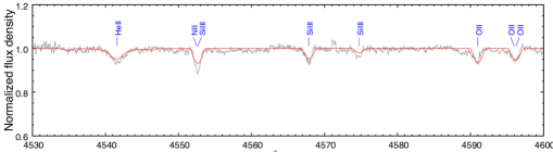
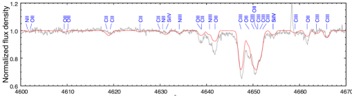
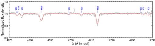
Figure 3: Comparison between the observed HDS (grey line) and the TLUSTY synthetic spectrum (red line) in the range between 4530 and 4740 Å. The absorption lines (except for H i) with the model predicted $EW\geq 10$ mÅ are indicated by the blue lines. The input parameters are listed in Table 5.

4.1 Stellar parameter derivations

We perform stellar absorption analysis of the HDS spectra taken on 2013 Oct 6 and Dec 10 using the non-local thermodynamic equilibrium (non-LTE) stellar atmosphere modelling code TLUSTY. We detect strong Si iii,iv and He ii absorption lines. From our TLUSTY modelling, $T_{\rm eff}$ of the central star is 28 100 K (Table 5), which is cooler than $T_{\rm eff}\geq 30\,000$ K in the O-type stars. Thus, we classify the stellar spectrum of SaSt 2-3 into early B-type giant B0-1II rather than O-type. Thus, we use comprehensive grid of 1540 metal line-blanketed, non-LTE, plane-parallel, hydrostatic model atmospheres of B-type stars BSTAR2006 by Lanz & Hubeny (2007).

We find the average nebular [Cl,S,Ar/H] of $-0.89~{}\pm~{}0.12$ (§ 3.5). Assuming that the metallicity $Z$ of the central star and the nebula is roughly the same as seen in the case of IC 418 by Morisset & Georgiev (2009), we adopt the $Z=0.1$ Z_☉ model grid from BSTAR2006. All of the initial abundances in this model grid are set to $\epsilon$(He) = 11.00 and [X/H] = –1 except for He. Based on the $Z=0.1$ Z_☉ model grid, we vary $\epsilon$(X) to yield each equivalent width ($EW$) of element X to compare with each $EW$(X) measured from the observed HDS spectra. Throughout our TLUSTY synthesis analysis, we do not set [He,C,N,O,Si/H] = –1 and we do not adopt the derived nebular He,C,N,O/H] as the stellar photospheric ones. Based on the measured $EW$ of the identified 9 He i,ii, 4 C iii,iv, 2 N ii,iii, 13 O ii, and 5 Si iii,iv absorption, we derive the photospheric He/C/N/O/Si abundances, microturbulent velocity ($v_{\rm t}$), rotational velocity ($v\,\sin(i)$; $i$ is the angle between the rotation axis and the line of sight), $T_{\rm eff}$, and $\log$ $g$ of the central star. These absorption lines are lesser affected by the nearby nebular lines and absorption lines of the other elements. As we report later, the central wavelength of the stellar absorption lines changes between observing dates whereas those of the nebular lines remain constant. Before analysis, we convert heliocentric wavelength frame of the HDS spectrum into rest frame using the radial velocity determined by the He ii 4686 Å for the 2013 Oct 6 data ($154.8~{}\pm~{}2.3$ km s^-1) and the He ii 5411 Å for the 2013 Dec 10 data ($182.3~{}\pm~{}4.0$ km s^-1).

First, we set the basic parameters characterising the stellar atmosphere, i.e., $Z$, $v_{\rm t}$, $T_{\rm eff}$, and $\log$ $g$. By setting $T_{\rm eff}=28\,000$ K and $\log\,g=3.10$ cm s^-2, we investigate $\epsilon$(O) versus selected 8 O ii lines’ $EW$ to determine $v_{\rm t}$ using SYNFIT. For each absorption, we set instrumental line broadening determined by measuring Th-Ar line widths. Since $v_{\rm t}\geq 10$ km s^-1 gives minimisation of the scatter in $\epsilon$(O) versus $EW$, we adopt $v_{\rm t}=10$ km s^-1. As a reference, Morisset & Georgiev (2009) adopted $v_{\rm t}=10$ km s^-1 for IC 418.

We determine $T_{\rm eff}$ and $\log\,g$ using the $T_{\rm eff}$-$\log\,g$ curves generated by the model atmosphere with $v_{\rm t}=10$ km s^-1, $Z$ = 0.1 Z_☉, and $\epsilon$(He) = 10.90. The $T_{\rm eff}$-$\log\,g$ curves are generated by the following process; for a fixed $T_{\rm eff}$, we vary $\log\,g$ from $2.90-3.30$ cm s^-2 in a constant 0.01 cm s^-2 step to find the best fit value for each observed He i,ii’s EW. We test the range of $T_{\rm eff}$ from $27\,500-28\,500$ K (200 K step).

Based on the determined $v_{\rm t}$, $T_{\rm eff}$, and $\log$ $g$, we further constrain $\epsilon$(He) and calculate $\epsilon$(C/N/O/Si) abundances by comparing the observed and model predicted $EW$s of each line by SYNABUND. We summarise the result in Table 5. In Appendix Table A4, we list the elemental abundances using each line. We adopt the average value as the representative abundance as listed in the last line of each element. The uncertainty of elemental abundances includes errors from the measured $EW$s, $T_{\rm eff}$, $\log$ $g$, and the uncertainty when we adopt the model atmosphere with the [Z/H] = $-0.90$ or $-1.10$ and when we assume the uncertainty of $v_{\rm t}$ of 2 km s^-1. We determine $v\,\sin(i)$ by line-profile fittings of the selected He i,ii and H i in $4000-4700$ Å using SYNFIT

Table 5: Summary of the set and derived parameters of the central star.

Parameter	Value	Parameter	Value
$T_{\rm eff}$ (K)	$28\,100~{}\pm~{}300$	$\epsilon$(He)	$10.99~{}\pm~{}0.09$
$\log\,g$ (cm s-2)	$3.11~{}\pm~{}0.05$	$\epsilon$(C)	$8.56~{}\pm~{}0.10$
$v_{\rm t}$ (km s-1)	$10~{}\pm~{}2$	$\epsilon$(N)	$7.26~{}\pm~{}0.16$
$v\,\sin(i)$ (km s-1)	$56~{}\pm~{}4$	$\epsilon$(O)	$8.10~{}\pm~{}0.17$
		$\epsilon$(Si)	$6.81~{}\pm~{}0.10$

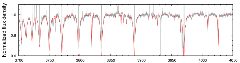
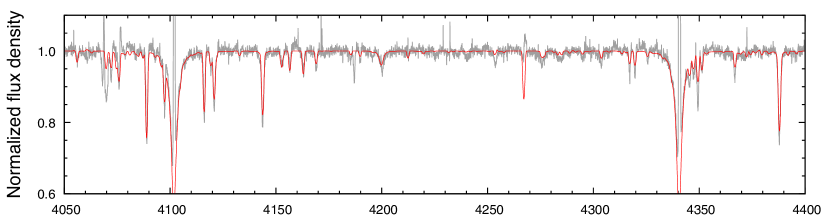
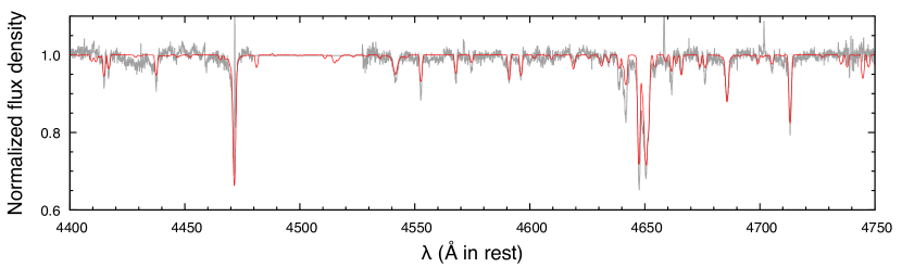
Figure 13: Comparison between the observed HDS (grey line) and the TLUSTY synthetic spectrum (red line) of SaSt 2-3. The input parameters are listed in Table 5.

In Fig. 3, we show the synthetic stellar spectrum generated using SYNSPEC. We identify the absorption lines (except for H i) with the model predicted $EW\geq 10$ mÅ by the blue lines. The synthetic spectrum in $3700-4750$ Å is presented in Appendix Fig. 13. Stellar Ne, S, Ar, Mg, Ca, and Ti ($\alpha$-elements) and Ni, Fe, and Zn are not derived in optical HDS spectra of SaSt 2-3. These abundances are not small and also they are very important in characterising the spectrum of the central star and its radiation hardness (in particular, X-ray to UV wavelength). We know that the central star radiation is suppressed by the metal line-blanket effect and also its is very important in subsequent Cloudy modelling. Thus, it is worth simulating these elements, too. We adopt the nebular Ne, S, Cl, and Ar abundances due to no detection of stellar absorption of these elements. We adopt $\epsilon$(Fe) = 6.38 ([Fe/H] = $-1.1$, see § 3.5). Based on the discussion in § 5, for the other elements up to Fe except for $\alpha$-elements Mg, Ca, and Ti, we adopt the predicted values by the AGB nucleosynthesis model of initially 1.25 M_☉ and $Z=0.001$ stars by Fishlock et al. (2014). For Mg, Ca, and Ti, we adopt $\epsilon$(Mg) = 6.80, $\epsilon$(Ca) = 5.43, and $\epsilon$(Ti) = 4.05, respectively (i.e., [Mg,Ca,Ti/H] = $-0.7$).

The stellar $\epsilon$(He/N/O) is in agreement with the nebular $\epsilon$(He/N/O) within their uncertainties. The stellar C/O ratio ($2.93~{}\pm~{}1.33$) indicates that SaSt 2-3 is definitely a C-rich PN. Based on the consistency between the stellar and the nebular elemental abundances, we obtain an expected CEL $\epsilon$(C) = $8.58~{}\pm~{}0.20$ using the CEL $\epsilon$(O) and the stellar C/O ratio.

4.2 Time variation of line-profile and radial velocity; Evidence of a binary central star

Our important discovery is that the central wavelength of the stellar absorption lines varies from date to date whereas there is no wavelength shift of the nebular emission lines.

We compute the heliocentric radial velocities $v_{r}$ of the central star via Fourier cross correlation between the observed spectra and the synthetic TLUSTY spectrum using FXCOR in IRAF. FXCOR calculates the velocity shift between two different spectra in the selected wavelength regions. Here, we select good S/N regions. In Table 6, we list $v_{r}$ and $v_{r}-v_{sys}$, where $v_{\rm sys}$ is the systemic radial velocity measured from the 128 nebular emission lines (+166.6 km s^-1, see § 3.1). In Fig. 4, we show the singlet He i 5015/7281 Å absorption and the TLUSTY synthetic spectrum as the guide.

We interpret that the radial velocity time-variation is caused by orbital motion in a binary system. Méndez et al. (1986) reported the photometric and radial velocity variations of the CSPN of C₆₀ PN IC 418. They measured the radial velocities using the stellar C iii 5695 Å and C iv 5801/11 Å. The systemic radial velocity was derived using the nebular [N ii] 5755 Å line. Later, Méndez (1989) concluded that the central star is not likely to be a binary because the orbital motion alone (if present) would not be enough to explain the observed variations. We note that the C iii 5695 Å and C iv 5801/11 Å lines are good indicators of the stellar activity (e.g., wind velocity) and these lines would be unlikely to give more accurate radial velocity of the central star. Thus, as far as we know, this would be the firm detection case of the binary central stars amongst all the C₆₀ PNe. Since we have only three periods of the binary motion, we do not determine any parameters of the binary central star yet.

We expected near-IR excess from the binary circumstellar disc from Otsuka et al. (2016) who detected near-IR excess in most of the SMC C₆₀ PNe and discussed possible links between near-IR excess, disc, and fullerene formation; since the ejected material from the central star can be stably harboured for a long time, even smaller molecules could aggregate into much larger molecules. However, in SaSt 2-3, we do not find near-IR excess in the observed SED (Fig. 1). No near-IR excess might mean a possibility of a nearly edge-on disc rather an inclined disc.

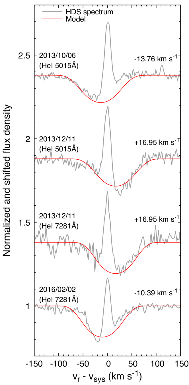
Figure 4: Time-variation of the singlet He i line-profiles taken in three nights. The systemic radial velocity ($v_{\rm sys}$) is +166.6 km s^-1 (§ 3.1). The synthetic spectrum is overplotted. The heliocentric radial velocity $v_{r}$ with respect to $v_{\rm sys}$ is indicated (see Table 6).

Table 6: Heliocentric radial velocity $v_{r}$ of the central star. The systemic radial velocity $v_{sys}$ is +166.6 km s^-1 (§ 3.1).

Obs Date	JD (– 2456000.0)	$v_{r}$ (km s-1)	$v_{r}-v_{sys}$ (km s-1)
2013/10/06	$573.096$	+152.8 $\pm$ 0.6	–13.76
2013/12/10	$637.917$	+183.6 $\pm$ 0.4	+16.95
2016/02/01	$1420.831$	+156.2 $\pm$ 0.6	–10.39

5 Comparison with AGB model predictions

Table 7: Comparison between the derived abundances and the predicted values by the AGB nucleosynthesis models of Fishlock et al. (2014) for 1.25 M_☉ stars with $Z=0.001$ and Karakas (2010) for 1.5 M_☉ stars with $Z=0.004$. The CEL $\epsilon$(C) is the predicted value by our analysis (§ 4.1).

X	Nebular	Stellar	1.25 M☉	1.50 M☉
			$Z=0.001$	$Z=0.004$
He	10.75 – 11.10	$10.99~{}\pm~{}0.09$	11.01	10.97
C(RL)	9.21 $\pm$ 0.12	$8.55~{}\pm~{}0.10$	8.56	8.46
C(CEL)	8.58 $\pm$ 0.20	$\cdots$
N	7.47 $\pm$ 0.06	$7.25~{}\pm~{}0.16$	7.26	7.65
O	8.11 $\pm$ 0.04	$8.10~{}\pm~{}0.17$	7.68	8.23
Ne	7.46 $\pm$ 0.04	$\cdots$	7.37	7.42
Si	$\cdots$	$6.81~{}\pm~{}0.10$	6.39	6.85
S	6.10 $\pm$ 0.03	$\cdots$	6.00	6.70
Cl	4.57 $\pm$ 0.07	$\cdots$	4.08	$\cdots$
Ar	5.66 $\pm$ 0.13	$\cdots$	5.28	$\cdots$
Fe	5.29 $\pm$ 0.06	$\cdots$	6.38	6.80

In Table 7, we compile the derived abundances. The nebular CEL $\epsilon$(C) is an expected value by our analysis (§ 4.1). As the comparisons, we list the AGB nucleosynthesis model predictions by Fishlock et al. (2014) for initially 1.25 M_☉ stars with $Z=0.001$ and Karakas (2010) for initially 1.50 M_☉ stars with $Z=0.004$. Note that Fishlock et al. (2014) and Karakas (2010) set the initial [X/H] to be –1.1 and –0.7, respectively. We calculate reduced chi-squared values ($\chi_{\nu}^{2}$, $\nu$ is degree of freedom) between the nebular $\epsilon$(X) and the AGB model predicted values for each of $1.00-3.25$ M_☉ star with $Z=0.001$ (9 models in total). We use $\chi_{\nu}^{2}$ as the guide to find out which AGB model’s predicted abundances is the closest to the derived abundances. The aim of this analysis is to infer the initial mass of the progenitor. We should note that these AGB grid models do not aim to explain the observed elemental abundances of SaSt 2-3. We exclude Fe in $\chi_{\nu}^{2}$ evaluation. We adopt the nebular $\epsilon$(X) values. For $\epsilon$(He) and $\epsilon$(C), we adopt $10.96~{}\pm~{}0.17$ (intermediate value, $9.10(-2)~{}\pm~{}3.52(-3)$) and $8.58~{}\pm~{}0.20$ (an expected nebular CEL C value, $3.80(-4)~{}\pm~{}1.76(-4)$), respectively.

Since the reduced-$\chi^{2}$ for the 1.25 M_☉ model marks the minimum ($\chi_{7}^{2}$ = 14 (= 99/($8-1$)) in 8 elements), this model is the closet to the derived $\epsilon$(X). $\chi_{4}^{2}$ is 17 (= 66/($5-1$)) limited to $\epsilon$(He/C/N/O/Ne). Next, we compare the AGB models for the same mass stars with $Z=0.004$ because these models could account for the derived abundances except for S (no predictions for Cl and Ar, however). The model for 1.5 M_☉ initial mass stars with $Z=0.004$ gives the closest fit to the observation ($\chi_{5}^{2}$ = 360 (= 1800/($6-1$))in 6 elements). Limited to $\epsilon$(He/C/N/O/Ne), $\chi_{4}^{2}$ is 7 (= 28/($5-1$)).

The B-type central star indicates that SaSt 2-3 is an extremely young PN and just finished the AGB phase. The presence of H absorption lines (Fig. 3) indicates that SaSt 2-3 did not experience very late thermal pulse evolution, so this PN is probably in the course of H-burning post-AGB evolution. According to the H-burning post-AGB evolution model of Vassiliadis & Wood (1994), stars with initially 1.5 M_☉ and $Z=0.004$ would evolve into hot stars with the core mass ($M_{\ast}$) of 0.64 M_☉. $L_{\ast}$ of such stars is $\sim$7380 L_☉ when $T_{\rm eff}$ is $\sim$28 100 K in $\sim$1050 years after the AGB phase. Whereas, we infer that 1.25 M_☉ stars with $Z=0.001$ would evolve into stars with $M_{\ast}$ of 0.649 M_☉; their $L_{\ast}$ and $T_{\rm eff}$ is $\sim$7765 L_☉ and $\sim$28 100 K, respectively in $\sim$1770 yrs after the AGB-phase based on the models of Fishlock et al. (2014) and Vassiliadis & Wood (1994). The main difference in the post-AGB evolution of 1.50 M_☉/$Z=0.004$ stars and 1.25 M_☉/$Z=0.001$ stars is evolutionary timescale.

Through these discussions, we summarise as follows. The $Z=0.001$ model gives the closest values to the derived elemental abundances, although there is systematically $\sim$0.3–0.4 dex discrepancy of $\epsilon$(O,Cl,Ar). The $Z=0.004$ model shows excellent fit to the derived nebular and stellar $\epsilon$(He/C/N/O/Si). Considering initial settings of [X/H] in the models, we conclude that the progenitor of SaSt 2-3 would be a $\sim$1.25 M_☉ star with initially $Z$$\sim$0.001 ([Fe/H]$\sim$–1.1) and [$\alpha$,Cl/Fe] $\sim$+0.3–0.4. This is consistent or comparable with the Galaxy chemical evolution model of Kobayashi et al. (2011); in the Galactic thick disc, the predicted [Si/Fe], [S/Fe], [Cl/Fe], and [Ar/Fe] are $\sim$+0.6, $\sim$+0.4, $\sim$–0.3, and $\sim$+0.3 in [Fe/H] $<-1$, respectively.

6 Photoionisation model

In the previous sections, we characterised the central star and dusty nebula. In this section, we build the photoionisation model using Cloudy and TLUSTY to be consistent with all the derived quantities, AGB nucleosynthesis model, and post-AGB evolution model. Below, we explain how to set each parameter in the model, and then we show the result.

6.1 Modelling approach

6.1.1 Distance

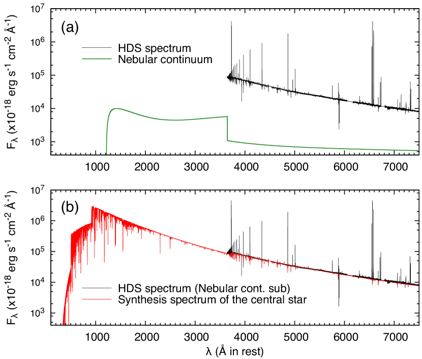
Figure 5: (Upper panel) The de-reddened HDS spectrum scaled up to the flux density at the APASS $Bg^{\prime}Vr^{\prime}i^{\prime}$ bands and the calculated nebular continuum by NEBCONT. (Lower panel) The synthetic spectrum of the central star by TLUSTY (§ 4.1) scaled to match the residual spectrum produced by subtracting the nebular continuum from the HDS spectrum.

Since the distance $D$ is an important parameter, we estimate it by our own method as explained below. We first extract the stellar spectrum from the observed HDS spectrum because the observed spectrum is the sum of the nebular emission lines and continuum and the central star’s continuum. For this purpose, we scale the HDS spectrum flux density to match the APASS $Bg^{\prime}Vr^{\prime}i^{\prime}$ bands. Then, we subtract the theoretically calculated nebular continuum from the scaled HDS spectrum. We utilise the NEBCONT code in the Dispo package of STARLINK v.2015A to generate the nebular continuum under adopting $I$(H$\beta$) = 1.57(–12) erg s^-1 cm^-2 (§ 3.2), $T_{\rm e}$ = 10⁴ K, $n_{\rm e}$ = 2000 cm^-3 (Table 2), and $n$(He⁺)/$n$(H⁺) = 1.09(–2) (Table A3). In Fig. 5(a), we show the scaled HDS spectrum and the synthetic nebular continuum. Fig. 5(b) displays the TLUSTY synthetic spectrum of the central star (in the case of $T_{\rm eff}=28\,100$ K) scaled to match the residual spectrum generated by subtracting the nebular continuum from the HDS spectrum.

Next, by integrating the scaled central star’s synthetic spectra in $T_{\rm eff}=27\,800-28\,400$ K (Table 5) by our TLUSTY analysis (§ 4.1) in over the wavelength, we obtain $L_{\ast}$ as a function of $D$ and $T_{\rm eff}$ for this $T_{\rm eff}$ range;

$$L_{\ast}=\left(48.56\cdot\left(T_{\rm eff}/10^{4}\right)-75.94\right)~{}\cdot~{}D_{\rm kpc}^{2}\,{\rm L}_{\sun}.$$ (2)

Assuming that the progenitor is an initially 1.25 M_☉/$Z=0.001$ star and its luminosity is currently 7765 L_☉ (§ 5), we obtain $D=9.90-12.76$ kpc. If we assume an initially 1.5 M_☉ progenitor star with $Z=0.004$, $D$ is $9.66-12.44$ kpc.

In our Cloudy model, we adopt $D=11.33$ kpc, which is the intermediate value of $D$ when we assume that the central star evolved from a star with initially 1.25 M_☉ and $Z=0.001$. Adopting our measured Galactocentric distance of 17.35 kpc, the predicted $\epsilon$(O/Ne/Cl/S/Ar) from the Galaxy $\epsilon$(O/Ne/Cl/S/Ar) gradient established amongst Galactic PN nebular abundances by Henry et al. (2004) are $8.33~{}\pm~{}0.21$, $7.61~{}\pm~{}0.35$, $6.22~{}\pm~{}0.25$, $4.67~{}\pm~{}0.34$, and $6.06~{}\pm~{}0.25$, respectively. These values are in line with the derived nebular abundances (Table 7). Our adopted $D=11.33$ kpc is in agreement with Frew et al. (2016), who reported $14.86~{}\pm~{}4.26$ kpc. Our derived $D$ is also comparable with the value ($14.31~{}\pm~{}8.54$ kpc) determined from the parallax measured using Gaia DR2 ($\sigma_{\pi}=0.0699~{}\pm~{}0.0417$ mas; Gaia Collaboration et al., 2018). Thus, we simultaneously justify our estimated $D$ and nebular $\epsilon$(O/Ne/Cl/S/Ar).

6.1.2 Central star

As input to Cloudy, we use the TLUSTY synthetic spectrum of the central star, adopting the parameters from Table 5. In our iterations here, we only vary $T_{\rm eff}$ in the range of $27\,800-28\,500$ K and $L_{\ast}$ in the range of $7300-8300$ L_☉.

6.1.3 Nebula geometry and boundary condition

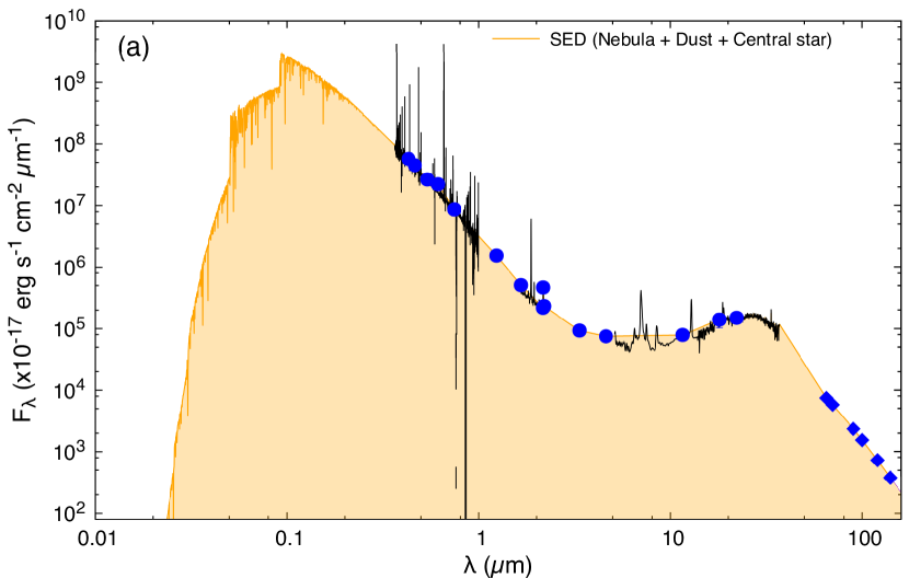
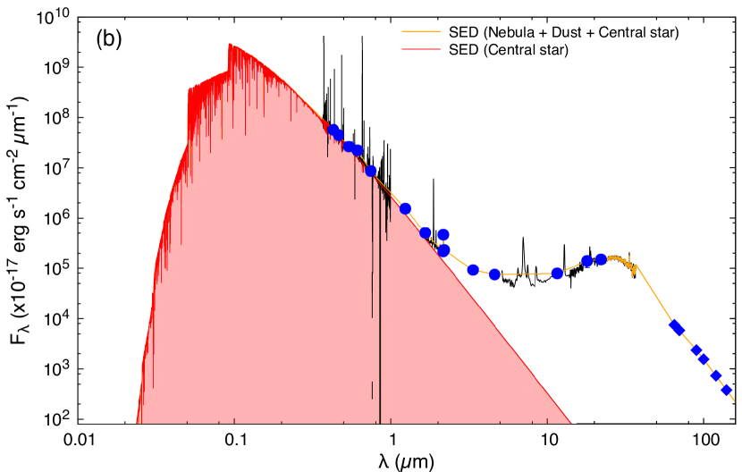
Figure 6: (Upper panel) SED based on the observed data (black lines and blue filled circles) and its interpolated curve (orange line). The far-IR flux density at 65, 90, 100, 120, and 140 µm (the blue diamonds) is an expected value. The integrated flux density between $\sim$5(–3) to 140 µm (indicated by the orange region) is $\sim$8215 L_☉ in $D=11.33$ kpc. (Lower panel) SED based on the observed data and its interpolated curve, and the synthetic spectrum of the central star. The integrated flux density of the central star within the same wavelength range (indicated by the red region) is $\sim$7765 L_☉ in $D=11.33$ kpc. See text in details.

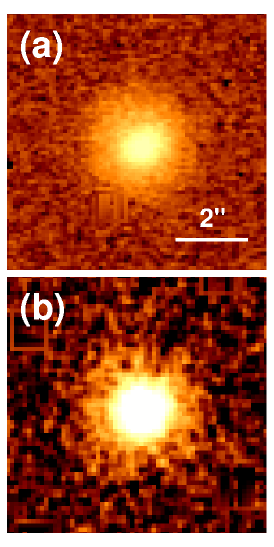
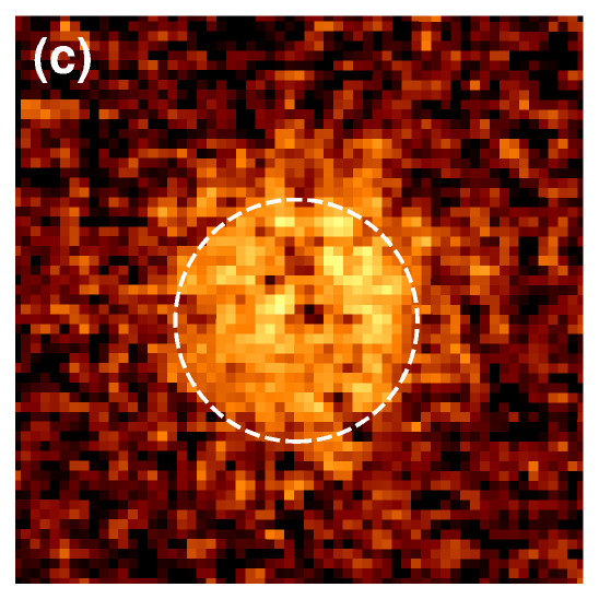
Figure 7: (LEFT two panels) The Br $\gamma$ and Br $\gamma$45 images of SaSt 2-3. (RIGHT panel) The Br $\gamma$ minus Br $\gamma$45 image. The radius of the dashed circle is 1.2″. North is up and east is left in these images.

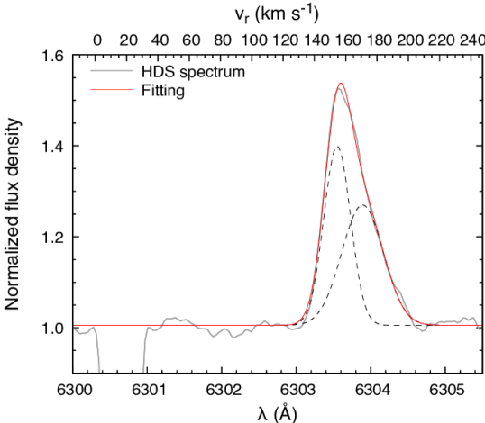
Figure 8: Fitting for the [O i] 6300 Å line. This line can be fitted with two Gaussian components (dashed lines). The red line is the sum of these components.

We plot the observed data and its interpolated curve in Fig. 6. The continuum spectrum in the wavelength $\lesssim 0.36$ µm corresponds to the sum of (1) the nebular continuum (green line in Fig. 5(a)) and (2) the synthetic spectrum of the central star (red line in Fig. 5(b)). The far-IR flux density at 65, 90, 100, 120, and 140 µm is an expected value obtained by fitting for the $15-40$ µm Spitzer/IRS spectrum.

We use Equations (2) and (3) Otsuka et al. (2014), who fitted the Spitzer/IRS spectra of Galactic C₆₀ PNe in $15-40$ µm with the synthetic absorption coefficient $Q_{\lambda}$ value. For SaSt 2-3, we set the minimum dust temperature = 20 K and adopt $p=q=2$ and $\alpha=0$ which are the same values used in Otsuka et al. (2014). From the fitting, we derive the maximum dust temperature of $136.2~{}\pm~{}0.4$ K, the expected $F_{\nu}$ at 65, 90, 100, 120, and 140 µm are 105.3, 63.5, 51.6, 35.0, and 24.6 mJy, respectively.

From integrating this SED (i.e., the orange region in Fig. 6(a)), we find a total luminosity of $\sim$8215 L_☉. The luminosity of each component is

Central star:

$\sim$7765 L_☉,

Nebular continuum + dust continuum:

$\sim$392 L_☉,

Nebular emission line:

$\sim$58 L_☉.

Here, the luminosity of nebular emission line is the sum of all the detected emission lines in the HDS and Spitzer spectra. We obtain $L_{\ast}$ of $\sim$7765 L_☉ by integrating flux density of the central star’s SED within the same wavelength range, indicated by the red region in Fig. 6(b). Thus, we find that only $\sim$6  percent of the central star’s radiation (= (392+58)/7765) seems to be absorbed by the nebula.

To check whether nebula boundary is determined by the power of the stellar radiation (i.e., ionisation bound) or material distribution (i.e., material bound), we tested both the ionisation boundary model and the material boundary model. The WHIRC Br$\gamma$ and Br$\gamma$45 images in Fig. 7 display the central bright region and the compact nebula. From the Br$\gamma$ – Br$\gamma$45 image (Fig. 7(c)), we measure the radius of the ionised nebula extended up to be 1.2″.

The material boundary model (the model calculation is stopped at the outer radius of 1.2″) gives a good fit except for underestimates of the [O i] and [N i] line fluxes. However, when we adopt an open geometry such as a cylinder in the ionisation boundary model (the model calculation is stopped when $T_{\rm e}$ is dropped down to $\sim$4000 K where most of the ionised species are not emitted), we explained well the balance between the input energy from the central star and the output energy from the nebula plus dust (i.e., $L_{\ast}\gg L_{\rm neb+dust}$) and the observed [O i] and [N i] line fluxes. Although the WHIRC images do not clearly show a cylinder or bipolar nebula, it is plausible judging from the [O i] 6300 Å line-profile. Fig. 8 shows the [O i] 6300 Å line-profile fitting by two Gaussian components with $v_{r}$ = +154.6 and +170.6 km s^-1 at the peak intensity of each component. The [O i] lines emitted from the most outer part of the nebula show blue-shifted asymmetry. Such asymmetric profiles are seen in e.g., PN Wray 16-423 (Otsuka, 2015); Wray16-423 has a bright cylindrical structure surrounded by an elliptically extended nebula shell.

From these discussions, we adopt the cylinder geometry with the height = 0.8″. We determined this scale height through a small grid model, and we found that the cylinder height $\geq 0.8$″ is necessary. We adopt ionisation bounded condition, assuming the ionisation front radius of 1.2″.

6.1.4 Elemental abundances and hydrogen density

We adopt the nebular value of $\epsilon$(N/O/Ne/S/Cl/Ar/Fe) (Table 7) as the initial value and then refine via model iterations within 0.2 dex of the input values so that the best-fit abundances would reproduce the observed emission line intensities. We adopt the nebular $\epsilon$(He) = 10.96 as the first guess, and vary it in range from 10.75 to 11.10. We keep an expected CEL $\epsilon$(C) = 8.58 (c.f. stellar $\epsilon$(C) = 8.55) and stellar $\epsilon$(Si) = 6.81 through the model iterations. For $\alpha$-elements Mg, Ca, and Ti (not derived, though), we fix the [Mg,Ca,Ti/Fe] = +0.3, where [Fe/H] is $-1.1$ (§ 5). We adopt a constant hydrogen number density ($n_{\rm H}$) radial profile. We first guess that $n_{\rm H}$ is equal to $n_{\rm e}$; we adopt the average $n_{\rm e}$ amongst the measured $n_{\rm e}$ except for $n_{\rm e}$([N i]) (Table  2), then we vary $n_{\rm H}$ to get the best fit.

6.1.5 Dust grains

We assume that the underlying continuum is due to graphite grains based on the fact that SaSt 2-3 shows the spectral signature of carbon-rich species.

We use the optical data of Martin & Rouleau (1991) for randomly oriented graphite spheres, and we assume the "$1/3-2/3$" approximation (Draine & Malhotra, 1993). We adopt the grain radius $a=0.05-0.25$ µm and $a^{-3.5}$ size distribution. If we set the smallest $a=0.005$ µm, the maximum grain temperature is over the sublimation temperature of 1750 K. Thus, we set the smallest $a=0.05$ µm. We resolve the size distribution into 20 bins (the smallest is $0.05-0.054$ µm and the largest is $\sim$$0.23-0.25$ µm). We do not attempt to fit the broad $6-9$ µm and 11 µm features because the carriers of these features are not determined yet and also these profiles are different from typical band profile of the polycyclic aromatic hydrocarbons (PAHs) in the same wavelengths.

6.2 Modelling results

The input parameters of the best fitting result and the derived quantities are summarised in Table 8. In total, we varied 12 parameters within a given range; $L_{\ast}$, $\epsilon$(He/N/O/Ne/S/Cl/Ar/Fe), inner radius ($r_{\rm in}$), $n_{\rm H}$, and grain abundance until $\chi_{\nu}^{2}$ calculated from $I$(H$\beta$), 76 emission line fluxes, 25 broadband fluxes, 4 mid-IR flux densities, and ionisation bound radius (i.e., outer radius $r_{\rm out}$). Since there is no observed far-IR data, we stop the model calculation at the ionisation front, where $T_{\rm e}$ is dropped down to $\sim$4000 K. To evaluate the goodness of the model fitting, we refer to $\chi_{\nu}^{2}$. For the [O i] and [N i] lines, we adopt 30 percent relative uncertainty because these lines are mostly from the PDRs. For the higher order Balmer lines H i (B24 - B14), we set 10 percent relative uncertainty by considering into account the uncertainty of these lines largely affected by the stellar absorption. The reduced-$\chi^{2}$ value in the best model is 12. The relatively large reduced-$\chi^{2}$ value even in the best fitting would be due to the uncertainty of the atomic data which we cannot control. Therefore, we conclude that our best fitting result reproduces observations very well. The predicted line fluxes, broadband fluxes, and flux densities are compiled in Appendix Table A5. For references, we list expected $F_{\nu}$ at 65, 90, 100, 120, and 140 $\mu$m obtained by fitting for the $15-40$ µm Spitzer/IRS spectrum (§ 6.1.3). In Figs. 9 and 10, we compare the model SED with the observed one.

Table 8: The best-fit model parameters of SaSt 2-3.

Central star	Value
$L_{\ast}$ / $T_{\rm eff}$ / $\log\,g$ / $D$	7400 L☉ / 28 170 K / 3.11 cm s-2 / 11.33 kpc
$M_{V}$ / $R_{\ast}$ /$m_{\ast}$	–2.10 / 3.606 R☉ / 0.611 M☉
Nebula	Value
Geometry	Cylinder with height = 0.8″ (8600 AU)
Radius	$r_{\rm in}$:0.006″ (63 AU), $r_{\rm out}$:1.25″ (14 162 AU)
$\epsilon$(X)	He:10.83, C:8.58, N:7.46, O:8.27, Ne:7.46,
	Mg:6.80, Si:6.84, S:6.10, Cl:4.51, Ar:5.65,
	Ca:5.43, Ti:4.05, Fe:5.41,
	Others: Fishlock et al. (2014)
$n_{\rm H}$	3098 cm-3
$\log$ $I$(H$\beta$)	–11.804 erg s-1 cm-2
$m_{g}$	6.13(–2) M☉
Dust	Value
Grain size	$0.05-0.25$ µm
$T_{d}$ / $m_{d}$ / DGR ($m_{d}$/$m_{g}$)	$66-909$ K / 2.08(–5) M☉ / 3.39(–4)

Note –

Nebular $\epsilon$(He/N/O/Ne/S/Cl/Ar/Fe) abundances derived by empirical method (§ 3.5) are $10.75-11.10$/7.47/8.11/7.46/6.10/4.57/5.66/5.29, respectively.

Table 9: Ionic abundance fraction predicted by our model and comparison between the predicted ICFs (ICF_model) and the empirically determined ICFs (ICF_emp).

X	X0	X+	X2+	X3+	ICFmodel	ICFemp
He	$0.845$	0.155	$<0.001$		6.70	$5.12-11.57$
C	$<0.001$	0.883	$0.116$	$<0.001$	8.61	$5.12~{}\pm~{}1.41$
N	$0.002$	0.948	$0.050$	$<0.001$	1.05	$1.04~{}\pm~{}0.13$
O	$0.010$	0.982	$0.008$	$<0.001$	1.01	1.00
Ne	$0.012$	0.988	$<0.001$	$<0.001$	1.01	1.00
S	$<0.001$	0.244	$0.756$	$<0.001$	1.00	1.00
Cl	$<0.001$	0.383	$0.617$	$<0.001$	1.00	1.00
Ar	$0.003$	0.867	$0.131$	$<0.001$	7.66	$5.12~{}\pm~{}1.41$
Fe	$<0.001$	0.062	$0.923$	$0.015$	1.08	$1.31~{}\pm~{}0.16$

In Fig. 11, we show the location of the CSPN predicted by our Cloudy model on the post-AGB evolutionary tracks for initially $Z=0.001$ and 1.0, 1.25, and 1.50 M_☉ (Vassiliadis & Wood, 1994). We generate this 1.25 M_☉ track by linear interpolation between the 1.00 and 1.50 M_☉ tracks of (Vassiliadis & Wood, 1994). Our Cloudy model predicts $L_{\ast}=7400$ L_☉, $T_{\rm eff}=28\,170$ K, and $m_{\ast}=0.611$ M_☉. $L_{\ast}$ and $m_{\ast}$ are justly close to predicted values ($\sim$7765 L_☉ and 0.649 M_☉) based on the models of initially 1.25 M_☉ stars with $Z=0.001$ (Vassiliadis & Wood, 1994; Fishlock et al., 2014). In Fig. 11, we plot the model results of Gesicki & Zijlstra (2007) and Otsuka et al. (2014) as well. These two models show a large discrepancy from the predicted post-AGB evolution track, but our model completely improves this.

Our model succeeds in reproducing the derived $\epsilon$(X), the volume average $T_{\rm e}$ (9150 K, while 8930 K in the observation), and $I$(H$\beta$). In Table 9, we present the fraction of each ion in each element. Except for C and Ar, the model predicted ICF is well consistent with the empirically determined ICF.

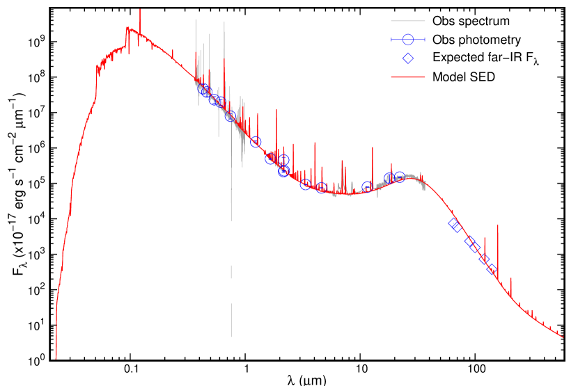
Figure 9: Comparison between the observed SED (blue circles and grey lines) and the SED predicted by the best fit model (red line). The spectral resolution ($R$) of the model SED is a constant 1000.

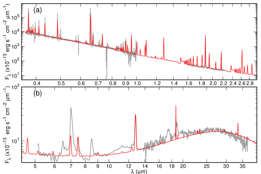
Figure 10: Comparison between the observed SED and the SED predicted by the best fit model in $0.35-3.0$ µm (upper panel) and in $4.4-40$ µm (lower panel). The legends in both panels are the same used in Fig. 9. $R$ of the model SED in $0.35-3.0$ µm is a constant 1000. $R$ is a constant 90 in $4.4-14$ µm (low-resolution module) and 570 in $14-40$ µm (high-resolution one), which correspond to the Spitzer/IRS resolution.

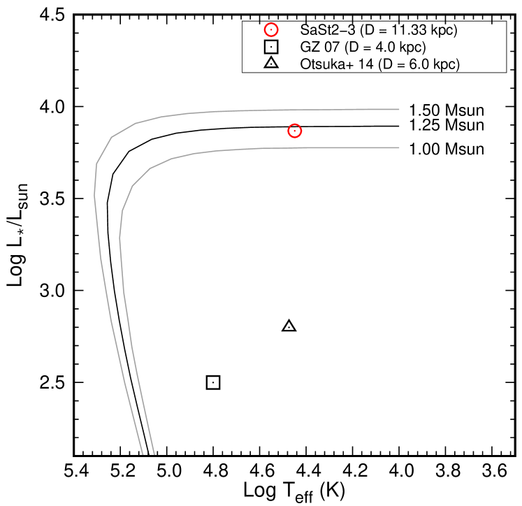
Figure 11: The location of the central star on the post-AGB evolutionary tracks for initially $Z=0.001$ and 1.0, 1.25, and 1.50 M_☉ (Vassiliadis & Wood, 1994). We generate this 1.25 M_☉ track by linear interpolation between the 1.00 and 1.50 M_☉ tracks of Vassiliadis & Wood (1994). For comparisons, we plot $T_{\rm eff}$ and $L_{\ast}$ of the central star derived by Gesicki & Zijlstra (2007) (GZ07, square; $T_{\rm eff}=63\,095$ K and $L_{\ast}=316$ L_☉ under $D=4$ kpc) and Otsuka et al. (2014) (Otsuka+ 14, triangle; $T_{\rm eff}=29\,750$ K and $L_{\ast}=630$ L_☉ under $D=6$ kpc).

The gas mass $m_{\rm g}$ is the sum of the ionised and neutral atomic/molecular gas species. Note that we stopped the model calculation at the ionisation front. Our $m_{\rm g}$ is $\sim$18 percent of the ejected mass at the last thermal pulse (TP) of 1.25 M_☉ initial mass stars with $Z=0.001$ (0.334 M_☉, Fishlock et al., 2014). If we increase the emitting volume by adopting a closed-geometry such as a spherical nebula, the situation is slightly improved (we trace $\sim$35 percent of the ejected mass) but the fitting model becomes worse as we explained. According to Fishlock et al. (2014), such stars experienced the superwind phase in the final few TPs during which the mass-loss rate reaches a plateau of $\sim$10^-5 M_☉ yr^-1. One might think that our underestimated $m_{\rm g}$ might be caused by excluding the neutral gas and molecular gas regions. However, it is unlikely that SaSt 2-3 has the molecular gas rich envelope because the molecular hydrogen H₂ lines in $K$-band are not detected (Lumsden et al., 2001). Indeed, we confirm this fact by analysis of the UKIRT CGS4 $HK$-band spectrum of SaSt 2-3 (Fig. 1). Since our $m_{\rm g}$ is greater than the ejected mass 2.7(–3) M_☉ at the last TP of initially 1.00 M_☉ stars with $Z=0.001$, we can conclude that the progenitor should be a $>1.00$ M_☉ initial mass star. Fishlock et al. (2014) predicts that 1.00 M_☉ stars lost the majority of its stellar envelope before it reaches the superwind phase. The 1.25 M_☉ progenitor that we infer might have experienced such mass loss. If this is true, non-detection of the H₂ lines might be because thin circumstellar envelope does not shield UV radiation from the CSPN and H₂ is dissociated. As an other explanation for the estimated small $m_{\rm g}$, the ejected mass during the AGB phase might be efficiently transported to the stellar surface of a companion star. Our small $m_{\rm g}$ would be largely improved by taking cold gas/dust components that can be traced by far-IR observation.

As presented in Fig. 10(b), our Cloudy model predicts an emission line around 7 µm. This line is the complex of the [Ar ii] 6.99 µm and H i 6.95/7.09 µm lines. In the Spitzer/IRS spectrum, we measure the total line-flux of the [Ar ii] 6.99 µm, H i 6.95/7.09 µm, and C₆₀ 7.0 µm to be $28.67~{}\pm~{}3.23$, where $I$(H$\beta$) = 100. The model predicts $I$([Ar ii] 6.99 µm + H i 6.95/7.09 µm)/$I$(H$\beta$) = 4.173 ($I$(H$\beta$) = 100). The contribution of the atomic line complex to the C₆₀ 7.0 µm band (14.6 $\%$) is not as significant as Otsuka et al. (2014) expected (30.3 $\%$). We estimate $I$(C₆₀ 7.0 µm)/$I$(H$\beta$) to be $24.5~{}\pm~{}2.8$.

7 Discussions

Table 10: Nebular and central star’s properties of C₆₀-containing PNe IC 418, Tc 1 and SaSt 2-3 and non C₆₀-containing C-rich PNe, IC 2165 and Me 2-1. $\epsilon$(He) in SaSt 2-3 listed in this table is the intermediate value of $\epsilon$(He) derived by empirical method. M_ini. is the initial mass of the progenitor inferred from the plot of $L_{\ast}$ and $T_{\rm eff}$ on the post-AGB evolutionary tracks (Fig. 12) based on Vassiliadis & Wood (1994).

Nebula	$\epsilon$(He)	$\epsilon$(C)	$\epsilon$(N)	$\epsilon$(O)	$\epsilon$(Ne)	$\epsilon$(S)	$\epsilon$(Cl)	$\epsilon$(Ar)	$\epsilon$(Fe)	$Z$	$\log\,L_{\ast}/L_{\sun}$	$T_{\rm eff}$ (K)	$\log\,g$ (cm s-2)	$M_{\rm ini.}$ (M☉)
IC 418	11.08	8.90	8.00	8.60	8.00	6.65	5.00	6.20	4.60	0.008	3.88	36 700	3.55	$\sim$1.8
Tc 1	10.92	8.56	7.56	8.41	7.80	6.45	4.97	6.08	5.19	0.004	3.85	32 000	3.30	$\sim$1.5
SaSt 2-3	10.96	8.58	7.47	8.11	7.46	6.10	4.57	5.66	5.29	0.001	3.87	28 170	3.11	$\sim$1.3
IC 2165	11.05	8.62	8.07	8.53	7.73	6.26	$\cdots$	6.00	$\cdots$	0.004	3.73	181 000	7.0	$\sim$2.1
Me 2-1	11.00	8.85	7.71	8.72	7.97	6.96	$\cdots$	6.20	$\cdots$	0.008	3.56	170 000	7.0	$\sim$1.8

Note –

We estimated $L_{\sun}$ of Tc 1 using $D=3.0$ kpc (cf. 2.67 kpc, Frew et al., 2013), a theoretical model spectrum of Lanz & Hubeny (2007) for O-type stars with $T_{\rm eff}=32\,000$ K, $\log\,g=3.3$ cm s^-2 (Mendez et al., 1992), and $Z=0.008$ to match with the interstellar extinction corrected HST/STIS spectrum of the central star (Khan & Worthey, 2018). We estimated $T_{\rm eff}$ of IC 2165 and Me 2-1 based the energy balance method of Dopita & Meatheringham (1991). $L_{\ast}$ is estimated using theoretical model spectra of Rauch (2003) with the derived $T_{\rm eff}$ and assumed $\log\,g=7.0$ cm s^-2 to match with the dereddened HST/WFPC2 F547M/F555W ($V$-band) magnitude of the central stars measured by Wolff et al. (2000), and $D$ of Frew et al. (2013).

7.1 Evolution of SaSt 2-3

Using the Galactic rotation velocity based on the distance scale of Cahn et al. (1992), van de Steene & Zijlstra (1995), and Zhang (1995), $v_{r}$(LSR) = 149.1 km s^-1, and $D=11.33$ kpc, we obtain ${\Delta}V=68.2-77.9$ km s^-1. The height above the Galactic plane $|z|$ is 1.13 kpc. These results are in agreement with the Type III PN classification of Quireza et al. (2007). ${\Delta}V$ and $|z|$ do not exceed 120 km s^-1 and 1.99 kpc for the Type IV PN classification of Quireza et al. (2007), respectively. The metallicity of SaSt 2-3 is much richer than typical halo PNe such as K 648, BoBn 1, and H 4-1 showing [Ar/H] $\lesssim-2$ (Otsuka et al., 2010; Otsuka et al., 2015; Otsuka & Tajitsu, 2013). Thus, we conclude that SaSt 2-3 belongs to the thick disc younger population and a Type III PN rather than a Type IV PN (Pereira & Miranda, 2007). Note that classification of PN type does not matter whether the central star is binary or not.

SaSt 2-3 would have evolved from a binary composed of a $\sim$1.25 M_☉ initial mass star and an companion star. However, any parameters on binary motion are unknown yet. According to the simulation using the binary_c code by Izzard et al. (2004), an initially 1.25 M_☉ single star with $Z=0.001$ will enter the PN phase within 3.5 Gyr after the progenitor was in the main-sequence. Perhaps, evolutionary time required to reach the AGB phase would be shortened by binary interaction (i.e., $<3.47$ Gyr).

SaSt 2-3 composes of a $\sim$0.61 M_☉ B-type cool central star with $T_{\rm eff}=28\,100$ K and a companion star. We find the Ca I absorption centred at 6616.62 Å and 6689.28 Å in heliocentric wavelength (6613.13 and 6685.6 Å in rest wavelength, respectively). $v_{r}$ using these two absorption lines is 165.5 km s^-1 and 152.1 km s^-1, respectively. These $v_{r}$ is close to $v_{r}$ of the central star (183.6 km s^-1, Table 6). Thus, we assume that these lines could be originated from the envelope in the companion star. However, since there is only one spectrum covering $6600-6690$ Å we have (Table 1), we do not yet find radial velocity variations of this absorption. We suppose that the companion star might be a F-K spectral type star in the main-sequence in terms of the initial mass by referring to De Marco et al. (2013).

7.2 Comparisons with non-C₆₀ and C₆₀-containing PNe

Our study can fully characterise the physical properties of SaSt 2-3. Thus, we are able to compare nebular elemental abundances and central star properties with those of other C₆₀ PNe, and we attempt to gain insights into the C₆₀ formation in PNe. For this purpose, we select C₆₀ PNe Tc 1 and IC 418 because they were previously modelled using Cloudy, and they have been extensively studied. In Table 10, we compile their properties. Due to the lack of existing UV spectra, the CEL $\epsilon$(C) in SaSt 2-3 is not determined yet. However, since we adopt an expected CEL $\epsilon$(C) (= (C/O)_∗ $\times$ O_CEL) from the stellar C/O ratio, the reliability of the discussion here is not compromised. We adopt the results of Tc 1 and IC 418 by Pottasch et al. (2011) and Morisset & Georgiev (2009), respectively. For Tc 1, since Pottasch et al. (2011) calculated $\epsilon$(Ar) by the sum of the Ar⁺ and Ar²⁺ abundances without subtracting C₆₀ 7.0 µm and H i lines from the complex line at 7 µm, their calculated $\epsilon$(Ar) is certainly overestimated. Therefore, we compute $\epsilon$(Ar) from Ar²⁺ (7.0(–7)) and ICF(Ar) = S/S²⁺ (1.71). $\epsilon$(He) in Tc 1 is predicted by their Cloudy model.

Comparisons with theoretical AGB nucleosynthesis models of Karakas (2010) indicate that the initial mass ($M_{\rm ini.}$) is $\sim$$1.90-2.10$ M_☉ for IC 418 and $\sim$$1.50-1.90$ M_☉ for Tc 1, respectively. From plots of $L_{\ast}$ and $T_{\rm eff}$ on the post-AGB evolutionary tracks based on Vassiliadis & Wood (1994) (Fig.12), we have the same estimate for IC 418 ($\sim$1.8 M_☉) and Tc 1 ($\sim$1.5 M_☉). Based on our estimates for the initial mass and metallicity, the age of IC 418 and Tc 1 after the main sequence is $\sim$$2-3$ Gyr. Thus, we attest that SaSt 2-3 is the most metal-deficient and oldest Galactic C₆₀ PN.

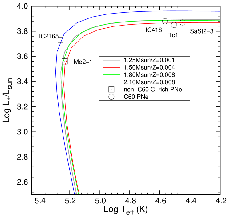
Figure 12: The location of C₆₀-containing PNe IC 418, Tc 1, and SaSt 2-3 and non-C₆₀ C-rich PNe IC 2165 and Me 2-1 on the post-AGB evolutionary tracks based on Vassiliadis & Wood (1994).

Our findings in elemental abundances are as follows; (i) the values of $\epsilon$(C) in these C₆₀ PNe are not peculiar values that can be explained by the AGB nucleosynthesis models, (ii) despite that the C₆₀ band strength in SaSt 2-3 and Tc 1 is much stronger than that in IC 418 (see Table 10 of Otsuka et al., 2014), and $\epsilon$(C) in Tc 1 and SaSt 2-3 is smaller than that in IC 418, and (iii) the C/O ratio (an indicator of the amount of the C-atoms unlocked in dust and molecules) in Tc 1 is smaller than that in IC 418. Supporting (i), non C₆₀-containing C-rich PNe IC 2165 (Miller et al., 2018) and Me 2-1 (Pottasch & Bernard-Salas, 2010) (they are selected based on metallicity and initial mass) show similar abundances (including $\epsilon$(C)) to C₆₀ PNe. The difference between non-C₆₀ and C₆₀ PNe is $T_{\rm eff}$ only, supporting that the weak radiation field from the central star is in favour of the C₆₀ formation. The time during which C₆₀ is present might be a short-lived phase that C-rich PNe go through, but we do not yet have firm observational evidence of this. These findings would result in our conclusion that the C₆₀ formation does not largely depend on the amount of the C-atoms produced during the AGB phase, and Tc 1 and SaSt 2-3 efficiently produced the C₆₀ molecule by some mechanisms not present in IC 418.

It is noticeable that Fe abundance is highly depleted in all C₆₀ PNe. The highly deficient Fe is possibly due to selective depletion in a binary disc (e.g., Otsuka et al., 2016, reference therein). If C₆₀ PNe have a disc around the central star, they can harbour mass-loss including AGB products for a long time and shield C₆₀ molecules from the intense central star’s UV radiation. Then, most of the Fe-atoms might be tied up in dust grains (e.g., FeO) within a disc. Accordingly, an environment suitable for large carbon molecule formation might be created. This would be in the case of SaSt 2-3. The central star of IC 418 would be not a binary (e.g., Méndez, 1989). There are no reports on the binary central star of Tc 1 so far.

If it is the case, is C₆₀ formation dependent on the central star’s properties and its surrounding environment, such as a binary disc? To answer this question, we need to calculate the mass of the C-atoms present in atomic gas, dust and C₆₀ by a fair means. From a more global perspective, the fraction of the C-atoms would be a critically important parameter to understand how much mass carbon PN progenitors had returned to their host galaxies. However, we find that the excitation diagram based on the observed C₆₀ 8.5/17.4/18.9 µm fluxes and the expected C₆₀ 7.0 µm flux ($I$(C₆₀ 7.0 µm)/$I$(H$\beta$) = $24.5~{}\pm~{}2.8$, see § 6.2) in SaSt 2-3 indicates non-LTE conditions. The same situation exists in other C₆₀ PNe including Tc 1 (Cami et al., 2010) and IC 418 (Otsuka et al., 2014). Therefore, we sought other ways not involving the excitation diagrams. Of these, the method proposed by Berné & Tielens (2012) is seemingly suitable to our aim; this method requires the observed/modelled IR SED, all four mid-IR C₆₀ band fluxes, and dust mass. These three parameters are already determined in SaSt 2-3 and IC 418.

In Table 11, we summarise the mass of the C-atoms present in atomic gas, dust, and C₆₀ in SaSt 2-3, IC 418, and Lin 49 in the SMC (as a comparison of the possible binary C₆₀ PN). For SaSt 2-3 and Lin 49, we obtain $I$(IR) by integrating the atomic gas emission free SED (generated by the Cloudy best model) in the range from 4 to 200 µm. Then, we calculate the total C₆₀ flux $I$(C₆₀) (Table A12). Finally, assuming that the dust and C₆₀ are emitted in the same regions, we estimate the C₆₀ mass (= $m_{\rm d}\times I$(C₆₀)/$I$(IR)). The column density and total number of C₆₀ in SaSt 2-3 are 8.57(+12) cm^-2 and 7.53(+47), respectively. By applying the method to IC 418 (but using the combined Infrared Space Observatory (ISO)/Short Wavelength Spectrometer (SWS)/Long-Wave Spectrometer (LWS) and Spitzer combined spectrum), we obtain their C₆₀ mass.

From this analysis, we quantitatively demonstrate that SaSt 2-3 and Lin 49 produced C₆₀ more efficiently than IC 418. Thus, we conclude that the C₆₀ formation depends upon the central star’s properties and its surrounding environment (e.g., a binary disc), rather than the amount of C-atoms.

Table 11: Mass of the C-atoms in each atomic gas, dust, and C₆₀.

Nebula	atomic C	graphite grains	C60	Mass frac.
	($\times 10^{-4}$ M☉)	($\times 10^{-5}$ M☉)	($\times 10^{-7}$ M☉)	of C60 (%)
IC 418	3.99	1.70	2.26	0.05
Lin 49	3.00	$4.15-4.29$	$3.05-4.64$	$0.09-0.14$
SaSt 2-3	2.17	2.08	4.53	0.19

Note –

Mass of C₆₀ is determined by (graphite grain mass for Lin 49 and SaSt 2-3) or (the total dust mass 7.76(–5) M${\sun}$ including graphite grain for IC 418; Gómez-Llanos et al. 2018) $\times~{}I$(C₆₀)/$I$(IR). $I$(C₆₀) is the total flux of the mid-IR C${60}$ bands measured by Otsuka et al. (2014, 1.03(–10) erg s^-1 cm^-2 for IC 418 using the ISO/SWS/LWS and Spitzer combined spectrum), Otsuka et al. (2016, 9.26(–14) erg s^-1 cm^-2 for Lin 49), and the present work for SaSt 2-3 (9.43(–13) erg s^-1 cm^-2). $I$(IR) in IC 418, Lin 49, and SaSt 2-3 is 3.53(–8), 1.26(–11) (two-shell model)/8.56(–12) (single shell model), and 4.33(–11) in erg s^-1 cm^-2, respectively.

8 Summary

We have studied the fullerene-containing PN SaSt 2-3 in order to investigate its physical properties and gain insights into the C₆₀ formation in PN progenitors. We derived the nine and four elemental abundances from nebular line and stellar absorption analysis, respectively. The derived elemental abundances indicate that the progenitor is an initially $\sim$1.25 M_☉ star with $Z=0.001$ and $\alpha$-element and Cl enhanced ([$\alpha$,Cl/Fe] $\sim$+0.3-0.4). The distance $D$ of 11.33 kpc is determined by comparing the derived luminosity as a function of $D$ and $T_{\rm eff}$ with the predicted luminosity by the post-AGB evolution model for the 1.25 M_☉ stars with $Z=0.001$. SaSt 2-3 is classified as part of the thick disc population with an early B-type central star with $T_{\rm eff}=28\,100$ K, $\log\,{g}=3.11$ cm s^-2, and the core-mass of $\sim$0.61 M_☉. We discovered the binary central star of SaSt 2-3 from time-variation of the stellar radial velocity. Further observations are necessary to understand the binary system. We built the comprehensive photoionisation model. The calculated gas mass is much smaller than the AGB model prediction for the single 1.25 M_☉ stars with $Z=0.001$. The lower gas mass could be due to the short duration time of the superwind phase or efficient mass-transfer into the stellar surface of the companion star during the AGB phase. From the simple analysis, we quantitatively demonstrate that SaSt 2-3 produced C₆₀ more efficiently than other C₆₀ PNe. The C₆₀ formation would depend on the central star’s properties and its surrounding environment. There might be a link between the C₆₀ formation efficiency and the binary central star. Spatially-resolved spectral maps of the atomic carbon, carbon dust, and C₆₀ are necessary to identify the locations of C₆₀ and investigate the abundance distribution of these species within dusty nebula. We succeed to demonstrate what type of and how much mass of stars can produce how much C₆₀ molecules. We will further investigate stellar/nebular properties and C₆₀ in order to find what parameters are of critical importance in the C₆₀ formation.

Appendix A Supporting results

The following tables and figure support our works.

Table A12: Identified emission lines in the HDS and IRS spectra. $f$($\lambda$) is reddening law of Cardelli et al. (1989), $F$($\lambda$) and $I$($\lambda$) are observed and interstellar extinction corrected line fluxes normalised to $F$(H$\beta$) and $I$(H$\beta$), respectively.

$\lambda_{\rm lab.}$ (Å)	Line	$f(\lambda)$	$F$($\lambda$)	$\delta$ $F$($\lambda$)	$I$($\lambda$)	$\delta$ $I$($\lambda$)
$3656.66$	B37	$0.336$	$0.015$	$0.010$	$0.019$	$0.013$
$3657.27$	B36	$0.336$	$0.062$	$0.019$	$0.077$	$0.024$
$3657.92$	B35	$0.336$	$0.048$	$0.013$	$0.060$	$0.017$
$3658.64$	B34	$0.336$	$0.076$	$0.012$	$0.094$	$0.017$
$3659.42$	B32	$0.336$	$0.131$	$0.015$	$0.162$	$0.023$
$3660.28$	B33	$0.335$	$0.162$	$0.014$	$0.201$	$0.024$
$3661.22$	B31	$0.335$	$0.265$	$0.021$	$0.330$	$0.038$
$3662.26$	B30	$0.335$	$0.324$	$0.028$	$0.402$	$0.048$
$3663.40$	B29	$0.335$	$0.377$	$0.032$	$0.469$	$0.055$
$3664.68$	B28	$0.334$	$0.762$	$0.052$	$0.945$	$0.101$
$3666.09$	B27	$0.334$	$0.676$	$0.049$	$0.839$	$0.092$
$3667.68$	B26	$0.334$	$0.623$	$0.039$	$0.773$	$0.080$
$3669.46$	B25	$0.334$	$0.581$	$0.032$	$0.721$	$0.071$
$3671.48$	B24	$0.333$	$0.593$	$0.029$	$0.735$	$0.070$
$3673.76$	B23	$0.333$	$0.733$	$0.030$	$0.909$	$0.083$
$3676.36$	B22	$0.332$	$0.739$	$0.033$	$0.916$	$0.085$
$3679.35$	B21	$0.332$	$0.844$	$0.031$	$1.046$	$0.094$
$3682.81$	B20	$0.331$	$0.897$	$0.034$	$1.111$	$0.100$
$3686.83$	B19	$0.330$	$1.121$	$0.031$	$1.388$	$0.119$
$3691.55$	B18	$0.329$	$1.184$	$0.023$	$1.465$	$0.122$
$3697.15$	B17	$0.328$	$1.298$	$0.027$	$1.605$	$0.134$
$3703.85$	B16	$0.327$	$1.778$	$0.031$	$2.196$	$0.181$
$3709.65$	He i	$0.326$	$0.039$	$0.013$	$0.049$	$0.016$
$3711.97$	B15	$0.325$	$1.665$	$0.032$	$2.054$	$0.169$
$3721.94$	B14	$0.323$	$2.167$	$0.040$	$2.671$	$0.218$
$3726.03$	[O ii]	$0.322$	$107.494$	$1.338$	$132.411$	$10.617$
$3728.81$	[O ii]	$0.322$	$74.678$	$0.644$	$91.955$	$7.314$
$3733.01$	He i	$0.321$	$0.071$	$0.010$	$0.088$	$0.014$
$3734.37$	B13	$0.321$	$2.375$	$0.036$	$2.922$	$0.235$
$3750.15$	B12	$0.317$	$3.125$	$0.027$	$3.836$	$0.301$
$3770.63$	B11	$0.313$	$4.076$	$0.033$	$4.991$	$0.386$
$3797.90$	B10	$0.307$	$5.102$	$0.035$	$6.224$	$0.472$
$3819.60$	He i	$0.302$	$0.089$	$0.011$	$0.108$	$0.015$
$3835.38$	B9 (H$\eta$)	$0.299$	$6.491$	$0.037$	$7.876$	$0.580$
$3889.05$	B8	$0.286$	$9.595$	$0.191$	$11.547$	$0.844$
$3918.97$	C ii	$0.279$	$0.065$	$0.011$	$0.078$	$0.014$
$3920.68$	C ii	$0.279$	$0.142$	$0.011$	$0.170$	$0.018$
$3970.07$	B7 (H$\epsilon$)	$0.266$	$14.294$	$0.071$	$16.977$	$1.113$
$4068.60$	[S ii]	$0.239$	$0.808$	$0.035$	$0.944$	$0.069$
$4101.73$	B6 (H$\delta$)	$0.230$	$23.318$	$0.106$	$27.051$	$1.531$
$4267.00$	C ii	$0.180$	$0.210$	$0.030$	$0.236$	$0.035$
$4340.46$	B5 (H$\gamma$)	$0.157$	$42.854$	$0.195$	$47.420$	$1.837$
$4471.47$	He i	$0.115$	$0.569$	$0.013$	$0.613$	$0.022$
$4571.10$	Mg i]	$0.084$	$0.106$	$0.019$	$0.112$	$0.020$
$4658.05$	[Fe iii]	$0.058$	$0.391$	$0.015$	$0.406$	$0.017$
$4701.53$	[Fe iii]	$0.045$	$0.093$	$0.008$	$0.096$	$0.009$
$4754.69$	[Fe iii]	$0.030$	$0.077$	$0.013$	$0.079$	$0.014$
$4769.43$	[Fe iii]	$0.025$	$0.025$	$0.008$	$0.025$	$0.008$
$4861.33$	B4 (H$\beta$)	$0.000$	$100.000$	$0.251$	$100.000$	$0.251$
$4881.00$	[Fe iii]	$-0.005$	$0.131$	$0.009$	$0.130$	$0.009$
$4888.87$	[Fe iii]	$-0.007$	$0.021$	$0.007$	$0.021$	$0.007$
$4921.93$	He i	$-0.016$	$0.130$	$0.008$	$0.129$	$0.008$
$4958.91$	[O iii]	$-0.026$	$1.127$	$0.008$	$1.109$	$0.011$
$5006.84$	[O iii]	$-0.038$	$3.408$	$0.015$	$3.326$	$0.034$
$5015.68$	He i	$-0.040$	$0.385$	$0.010$	$0.375$	$0.011$
$5055.98$	Si ii	$-0.050$	$0.097$	$0.031$	$0.094$	$0.030$
$5067.52$	Ni iii	$-0.052$	$0.065$	$0.010$	$0.062$	$0.009$
$5197.90$	[N i]	$-0.082$	$0.059$	$0.022$	$0.056$	$0.021$
$5200.26$	[N i]	$-0.083$	$0.055$	$0.015$	$0.052$	$0.014$
$5270.40$	[Fe iii]	$-0.098$	$0.183$	$0.011$	$0.172$	$0.011$
$5273.24$	Ne ii	$-0.098$	$0.031$	$0.012$	$0.029$	$0.011$
$5517.72$	[Cl iii]	$-0.145$	$0.128$	$0.013$	$0.116$	$0.012$
$5537.89$	[Cl iii]	$-0.149$	$0.122$	$0.006$	$0.111$	$0.007$
$5754.64$	[N ii]	$-0.185$	$1.489$	$0.017$	$1.322$	$0.062$
$5875.60$	He i	$-0.203$	$1.786$	$0.029$	$1.566$	$0.082$
$5886.05$	C ii	$-0.205$	$0.061$	$0.010$	$0.054$	$0.009$
$5891.60$	C ii	$-0.205$	$0.056$	$0.008$	$0.049$	$0.007$
$5912.58$	C i	$-0.208$	$0.058$	$0.005$	$0.051$	$0.005$
$5931.78$	N ii	$-0.211$	$0.068$	$0.008$	$0.059$	$0.007$
$5950.71$	Fe iii	$-0.214$	$0.040$	$0.009$	$0.035$	$0.008$
$6300.30$	[O i]	$-0.263$	$0.638$	$0.018$	$0.538$	$0.038$
$6312.10$	[S iii]	$-0.264$	$0.212$	$0.013$	$0.179$	$0.016$
$6347.03$	Ni ii	$-0.269$	$0.070$	$0.010$	$0.059$	$0.009$
$6363.78$	[O i]	$-0.271$	$0.195$	$0.014$	$0.164$	$0.016$

Table A1: Continued.

$\lambda_{\rm lab.}$ (Å)	Line	$f(\lambda)$	$F$($\lambda$)	$\delta$ $F$($\lambda$)	$I$($\lambda$)	$\delta$ $I$($\lambda$)
$6379.58$	O ii	$-0.273$	$0.098$	$0.023$	$0.082$	$0.020$
$6461.95$	C ii	$-0.284$	$0.074$	$0.009$	$0.061$	$0.008$
$6548.04$	[N ii]	$-0.296$	$45.988$	$0.395$	$37.985$	$2.778$
$6562.80$	B3 (H$\alpha$)	$-0.298$	$375.888$	$1.958$	$310.085$	$22.731$
$6578.05$	C ii	$-0.300$	$0.317$	$0.008$	$0.261$	$0.020$
$6583.46$	[N ii]	$-0.300$	$138.238$	$1.323$	$113.836$	$8.471$
$6678.15$	He i	$-0.313$	$0.588$	$0.012$	$0.480$	$0.038$
$6716.44$	[S ii]	$-0.318$	$4.770$	$0.047$	$3.884$	$0.306$
$6730.81$	[S ii]	$-0.320$	$7.203$	$0.078$	$5.857$	$0.465$
$7065.18$	He i	$-0.364$	$0.494$	$0.011$	$0.391$	$0.036$
$7135.80$	[Ar iii]	$-0.374$	$0.740$	$0.009$	$0.581$	$0.054$
$7231.32$	C ii	$-0.387$	$0.352$	$0.018$	$0.274$	$0.024$
$7236.42$	C ii	$-0.387$	$0.741$	$0.034$	$0.576$	$0.042$
$7281.35$	He i	$-0.393$	$0.159$	$0.010$	$0.123$	$0.014$
$7318.92$	[O ii]	$-0.398$	$1.465$	$0.061$	$1.132$	$0.120$
$7319.99$	[O ii]	$-0.398$	$4.560$	$0.057$	$3.524$	$0.348$
$7329.66$	[O ii]	$-0.400$	$2.382$	$0.026$	$1.839$	$0.182$
$7330.73$	[O ii]	$-0.400$	$2.460$	$0.029$	$1.899$	$0.188$
$7751.10$	[Ar iii]	$-0.455$	$0.187$	$0.009$	$0.139$	$0.017$
$7769.23$	Ca i	$-0.458$	$0.122$	$0.007$	$0.091$	$0.012$
$7771.94$	O i	$-0.458$	$0.084$	$0.006$	$0.063$	$0.008$
$7874.65$	[Fe ii]	$-0.471$	$0.032$	$0.004$	$0.023$	$0.004$
$8240.19$	P45	$-0.515$	$0.067$	$0.008$	$0.048$	$0.008$
$8241.88$	P44	$-0.516$	$0.090$	$0.008$	$0.064$	$0.010$
$8243.69$	P43	$-0.516$	$0.055$	$0.006$	$0.039$	$0.007$
$8245.64$	P42	$-0.516$	$0.023$	$0.005$	$0.016$	$0.004$
$8247.73$	P41	$-0.516$	$0.071$	$0.006$	$0.051$	$0.008$
$8249.97$	P40	$-0.517$	$0.037$	$0.003$	$0.027$	$0.004$
$8252.40$	P39	$-0.517$	$0.077$	$0.008$	$0.055$	$0.009$
$8255.02$	P38	$-0.517$	$0.093$	$0.008$	$0.066$	$0.010$
$8257.85$	P37	$-0.517$	$0.093$	$0.007$	$0.066$	$0.010$
$8260.93$	P36	$-0.518$	$0.103$	$0.010$	$0.074$	$0.012$
$8264.28$	P35	$-0.518$	$0.107$	$0.009$	$0.076$	$0.012$
$8267.94$	P34	$-0.519$	$0.114$	$0.008$	$0.082$	$0.012$
$8271.93$	P33	$-0.519$	$0.118$	$0.012$	$0.084$	$0.014$
$8276.31$	P32	$-0.520$	$0.120$	$0.011$	$0.086$	$0.014$
$8281.12$	P31	$-0.520$	$0.114$	$0.010$	$0.081$	$0.013$
$8286.43$	P30	$-0.521$	$0.135$	$0.011$	$0.096$	$0.015$
$8292.31$	P29	$-0.521$	$0.190$	$0.012$	$0.135$	$0.019$
$8298.83$	P28	$-0.522$	$0.164$	$0.010$	$0.117$	$0.017$
$8306.11$	P27	$-0.523$	$0.207$	$0.012$	$0.148$	$0.021$
$8333.78$	P24	$-0.526$	$0.307$	$0.017$	$0.218$	$0.031$
$8340.80$	C ii	$-0.527$	$0.018$	$0.005$	$0.013$	$0.004$
$8345.47$	P23	$-0.527$	$0.296$	$0.017$	$0.211$	$0.030$
$8359.00$	P22	$-0.529$	$0.385$	$0.021$	$0.274$	$0.038$
$8374.48$	P21	$-0.531$	$0.366$	$0.020$	$0.260$	$0.037$
$8392.40$	P20	$-0.533$	$0.382$	$0.020$	$0.271$	$0.038$
$8413.32$	P19	$-0.535$	$0.449$	$0.021$	$0.318$	$0.044$
$8502.48$	P16	$-0.544$	$0.668$	$0.031$	$0.470$	$0.067$
$8665.02$	P13	$-0.560$	$1.274$	$0.057$	$0.887$	$0.128$
$8750.47$	P12	$-0.568$	$1.558$	$0.069$	$1.079$	$0.158$
$8776.83$	He i	$-0.571$	$0.046$	$0.005$	$0.032$	$0.006$
$8862.78$	P11	$-0.578$	$1.903$	$0.085$	$1.309$	$0.195$
$9014.91$	P10	$-0.590$	$2.554$	$0.113$	$1.744$	$0.264$
$9068.60$	[S iii]	$-0.594$	$3.789$	$0.170$	$2.581$	$0.394$
$9123.60$	[Cl ii]	$-0.598$	$0.128$	$0.010$	$0.087$	$0.014$
$9545.97$	P8	$-0.626$	$4.546$	$0.202$	$3.033$	$0.486$

Table A1: Continued.

$\lambda_{\rm lab.}$ (Å)	Line	$f(\lambda)$	$F$($\lambda$)	$\delta$ $F$($\lambda$)	$I$($\lambda$)	$\delta$ $I$($\lambda$)
$70000.0$	C60/[Ar ii]/H i				$28.665$	$3.226$
$74578.2$	H i				$3.102$	$0.226$
$85000.0$	C60				$7.003$	$0.545$
$89889.3$	[Ar iii]				$0.757$	$0.145$
$123800.0$	H i				$1.029$	$0.271$
$128100.6$	[Ne ii]				$20.607$	$1.555$
$174000.0$	C60/C70				$12.131$	$1.654$
	C60				$9.399$	$1.282$
$187079.3$	[S iii]				$5.263$	$0.724$
$189000.0$	C60/C70				$<21.253$
	C60				$<19.188$
$334719.0$	[S iii]				$4.004$	$0.857$

Note –

We measured the flux of the C_60,70 18.9 µm by adopting FWHM of 0.347 µm measured in Tc 1 (Otsuka et al., 2014) because this line seems to be partially lacked due to spike noise. We estimated the expected solo intensity of the C₆₀ 17.4/18.9 µm using the C₆₀/C₇₀ ratio at 17.4 µm = 3.44 and the C₆₀/C₇₀ ratio at 18.9 µm = 9.29 measured in Tc 1 (Cami et al., 2010).

Table A2: Broadband flux density of SaSt 2-3.

Band	$\lambda_{\rm c}$	$F_{\lambda}$ (reddened)	$I_{\lambda}$ (de-reddened)
		(erg s-1 cm-2 µm-1)	(erg s-1 cm-2 µm-1)
$B$	0.4297 µm	$2.24(-10)~{}\pm~{}5.99(-12)$	$4.75(-10)~{}\pm~{}1.41(-10)$
$g{{}^{\prime}}$	0.4640 µm	$1.93(-10)~{}\pm~{}1.42(-12)$	$3.81(-10)~{}\pm~{}1.03(-10)$
$V$	0.5394 µm	$1.31(-10)~{}\pm~{}3.25(-12)$	$2.29(-10)~{}\pm~{}5.14(-11)$
$r{{}^{\prime}}$	0.6122 µm	$1.05(-10)~{}\pm~{}2.61(-12)$	$1.96(-10)~{}\pm~{}3.82(-11)$
$i{{}^{\prime}}$	0.7440 µm	$3.89(-11)~{}\pm~{}3.29(-12)$	$7.89(-11)~{}\pm~{}1.35(-11)$
$J$	1.235 µm	$1.27(-11)~{}\pm~{}3.03(-13)$	$1.48(-11)~{}\pm~{}9.94(-13)$
$H$	1.662 µm	$4.49(-12)~{}\pm~{}1.24(-13)$	$4.95(-12)~{}\pm~{}2.36(-13)$
$Ks$	2.159 µm	$2.01(-12)~{}\pm~{}6.86(-14)$	$2.15(-12)~{}\pm~{}9.13(-14)$
Br$\gamma$	2.162 µm	$4.29(-12)~{}\pm~{}7.66(-13)$	$4.57(-12)~{}\pm~{}8.25(-13)$
Br$\gamma$45	2.188 µm	$2.15(-12)~{}\pm~{}4.14(-14)$	$2.28(-12)~{}\pm~{}7.21(-14)$
W1	3.353 µm		$9.28(-13)~{}\pm~{}1.97(-14)$
W2	4.602 µm		$7.49(-13)~{}\pm~{}1.45(-14)$
W3	11.56 µm		$7.87(-13)~{}\pm~{}1.09(-14)$
L18W	18.00 µm		$1.40(-12)~{}\pm~{}3.71(-13)$
W4	22.09 µm		$1.50(-12)~{}\pm~{}3.04(-14)$

Table A3: Ionic abundances of SaSt 2-3 using nebular emission lines.

Ion(Xm+)	$\lambda_{\rm lab.}$	$I$($\lambda$) ($I$(H$\beta$) = 100)	$n$(Xm+)/$n$(H+)
He+	4471.47 Å	$0.613~{}\pm~{}0.022$	$1.11(-2)~{}\pm~{}4.43(-4)$
	4921.93 Å	$0.129~{}\pm~{}0.008$	$9.44(-3)~{}\pm~{}6.10(-4)$
	5015.68 Å	$0.375~{}\pm~{}0.011$	$1.20(-2)~{}\pm~{}4.04(-4)$
	5875.60 Å	$1.566~{}\pm~{}0.082$	$9.58(-3)~{}\pm~{}5.33(-4)$
	6678.15 Å	$0.480~{}\pm~{}0.038$	$1.19(-2)~{}\pm~{}9.72(-4)$
	7065.18 Å	$0.391~{}\pm~{}0.036$	$6.49(-3)~{}\pm~{}6.06(-4)$
	7281.35 Å	$0.123~{}\pm~{}0.014$	$1.06(-2)~{}\pm~{}1.21(-3)$
			${\bf 1.09(-2)}~{}\pm~{}{\bf 2.28(-4)}$
C2+	4267.00 Å	$0.236~{}\pm~{}0.035$	$2.39(-4)~{}\pm~{}3.58(-5)$
	5891.60 Å	$0.049~{}\pm~{}0.007$	$3.35(-4)~{}\pm~{}4.56(-5)$
	6461.95 Å	$0.061~{}\pm~{}0.008$	$6.03(-4)~{}\pm~{}8.07(-5)$
	6578.05 Å	$0.261~{}\pm~{}0.020$	$3.16(-4)~{}\pm~{}2.60(-5)$
	7231.34 Å	$0.274~{}\pm~{}0.024$	$6.11(-4)~{}\pm~{}8.85(-5)$
	7236.42 Å	$0.576~{}\pm~{}0.042$	$6.68(-4)~{}\pm~{}6.13(-5)$
			${\bf 3.14(-4)}~{}\pm~{}{\bf 2.49(-5)}$
N0	5197.90 Å	$0.056~{}\pm~{}0.021$	$7.60(-7)~{}\pm~{}2.85(-7)$
	5200.26 Å	$0.052~{}\pm~{}0.014$	$4.04(-7)~{}\pm~{}1.35(-7)$
			${\bf 5.82(-7)}~{}\pm~{}{\bf 2.51(-7)}$
N+	5754.64 Å	$1.322~{}\pm~{}0.062$	$2.88(-5)~{}\pm~{}5.08(-6)$
	6548.04 Å	$37.985~{}\pm~{}2.778$	$2.83(-5)~{}\pm~{}2.93(-6)$
	6583.46 Å	$113.836~{}\pm~{}8.471$	$2.86(-5)~{}\pm~{}3.00(-6)$
			${\bf 2.85(-5)}~{}\pm~{}{\bf 1.94(-6)}$
O0	6300.30 Å	$0.538~{}\pm~{}0.038$	$4.37(-6)~{}\pm~{}1.25(-6)$
	6363.78 Å	$0.164~{}\pm~{}0.016$	$4.16(-6)~{}\pm~{}1.22(-6)$
			${\bf 4.26(-6)}~{}\pm~{}{\bf 8.72(-7)}$
O+	3726.03 Å	$132.411~{}\pm~{}10.617$	$1.29(-4)~{}\pm~{}2.56(-5)$
	3728.81 Å	$91.955~{}\pm~{}7.314$	$1.25(-4)~{}\pm~{}1.38(-5)$
	7318.92 Å	$1.132~{}\pm~{}0.120$	$1.38(-4)~{}\pm~{}5.23(-5)$
	7319.99 Å	$3.524~{}\pm~{}0.348$	$1.37(-4)~{}\pm~{}5.16(-5)$
	7329.66 Å	$1.839~{}\pm~{}0.182$	$1.35(-4)~{}\pm~{}5.11(-5)$
	7330.73 Å	$1.899~{}\pm~{}0.188$	$1.41(-4)~{}\pm~{}5.31(-5)$
			${\bf 1.28(-4)}~{}\pm~{}{\bf 1.10(-5)}$
O2+	4958.91 Å	$1.109~{}\pm~{}0.011$	$1.68(-6)~{}\pm~{}6.82(-7)$
	5006.84 Å	$3.326~{}\pm~{}0.034$	$1.75(-6)~{}\pm~{}7.08(-7)$
			${\bf 1.72(-6)}~{}\pm~{}{\bf 4.91(-7)}$
Ne+	12.81 µm	$20.607~{}\pm~{}1.555$	$2.91(-5)~{}\pm~{}2.85(-6)$
S+	4068.60 Å	$0.944~{}\pm~{}0.069$	$6.22(-7)~{}\pm~{}1.08(-7)$
	6716.44 Å	$3.884~{}\pm~{}0.306$	$6.47(-7)~{}\pm~{}6.72(-8)$
	6730.81 Å	$5.857~{}\pm~{}0.465$	$6.38(-7)~{}\pm~{}7.27(-8)$
			${\bf 6.39(-7)}~{}\pm~{}{\bf 4.49(-8)}$
S2+	18.71 µm	$5.263~{}\pm~{}0.724$	$6.08(-7)~{}\pm~{}9.80(-8)$
	33.47 µm	$4.004~{}\pm~{}0.857$	$5.93(-7)~{}\pm~{}1.63(-7)$
	6312.10 Å	$0.179~{}\pm~{}0.016$	$5.84(-7)~{}\pm~{}3.00(-7)$
	9068.60 Å	$2.581~{}\pm~{}0.394$	$7.28(-7)~{}\pm~{}2.17(-7)$
			${\bf 6.18(-7)}~{}\pm~{}{\bf 7.57(-8)}$
Cl+	9123.60 Å	$0.087~{}\pm~{}0.014$	$1.74(-8)~{}\pm~{}3.20(-9)$
Cl2+	5517.72 Å	$0.116~{}\pm~{}0.012$	$2.12(-8)~{}\pm~{}8.45(-9)$
	5537.89 Å	$0.111~{}\pm~{}0.007$	$1.87(-8)~{}\pm~{}5.29(-9)$
			${\bf 1.94(-8)}~{}\pm~{}{\bf 4.48(-9)}$
Ar2+	8.99 µm	$0.757~{}\pm~{}0.145$	$8.79(-8)~{}\pm~{}1.74(-8)$
	7135.80 Å	$0.581~{}\pm~{}0.054$	$9.30(-8)~{}\pm~{}2.58(-8)$
	7751.10 Å	$0.139~{}\pm~{}0.017$	$9.29(-8)~{}\pm~{}2.68(-8)$
			${\bf 9.02(-8)}~{}\pm~{}{\bf 1.27(-8)}$
Fe2	4658.05 Å	$0.406~{}\pm~{}0.017$	$1.93(-7)~{}\pm~{}2.49(-8)$
	4701.53 Å	$0.096~{}\pm~{}0.009$	$1.45(-7)~{}\pm~{}2.40(-8)$
	4754.69 Å	$0.079~{}\pm~{}0.014$	$2.00(-7)~{}\pm~{}4.24(-8)$
	4769.43 Å	$0.025~{}\pm~{}0.008$	$1.10(-7)~{}\pm~{}3.71(-8)$
	4881.00 Å	$0.130~{}\pm~{}0.009$	$1.09(-7)~{}\pm~{}1.99(-8)$
	5270.40 Å	$0.172~{}\pm~{}0.011$	$1.61(-7)~{}\pm~{}2.06(-8)$
			${\bf 1.48(-7)}~{}\pm~{}{\bf 1.03(-8)}$

Table A4: The measurements of the equivalent width ($EW$) of the stellar absorption and the derived elemental abundances.

Line	$\lambda_{\rm lab.}$ (Å)	$EW$ (mÅ)	$n$(X)/$n$(H)	$\epsilon$(X)
He i	3652.90	$29.24~{}\pm~{}1.87$	$8.92(-2)~{}\pm~{}2.77(-2)$	$10.95~{}\pm~{}0.14$
	3867.45	$104.20~{}\pm~{}1.30$	$9.30(-2)~{}\pm~{}1.41(-2)$	$10.97~{}\pm~{}0.07$
	4009.24	$188.70~{}\pm~{}1.56$	$7.85(-2)~{}\pm~{}9.76(-3)$	$10.89~{}\pm~{}0.05$
	4120.78	$184.40~{}\pm~{}2.10$	$1.20(-1)~{}\pm~{}2.12(-2)$	$11.08~{}\pm~{}0.08$
	4143.68	$266.70~{}\pm~{}1.65$	$1.13(-1)~{}\pm~{}1.47(-2)$	$11.05~{}\pm~{}0.06$
	4168.99	$39.69~{}\pm~{}1.48$	$8.60(-2)~{}\pm~{}1.96(-2)$	$10.93~{}\pm~{}0.10$
He ii	4541.62	$129.90~{}\pm~{}2.34$	$1.01(-1)~{}\pm~{}2.23(-2)$	$11.01~{}\pm~{}0.10$
	4685.71	$210.00~{}\pm~{}1.96$	$9.85(-2)~{}\pm~{}2.12(-2)$	$10.99~{}\pm~{}0.09$
	5411.52	$136.90~{}\pm~{}2.21$	$9.85(-2)~{}\pm~{}2.27(-2)$	$10.99~{}\pm~{}0.10$
			${\bf 9.76(-2)}~{}\pm~{}{\bf 1.93(-3)}$	${\bf 10.99}~{}\pm~{}{\bf 0.09}$
C iii	4156.56	$65.84~{}\pm~{}1.68$	$3.83(-4)~{}\pm~{}8.75(-5)$	$8.58~{}\pm~{}0.10$
	4162.96	$75.54~{}\pm~{}1.79$	$3.39(-4)~{}\pm~{}7.42(-5)$	$8.53~{}\pm~{}0.10$
	4665.92	$67.63~{}\pm~{}1.49$	$3.47(-4)~{}\pm~{}7.07(-5)$	$8.54~{}\pm~{}0.09$
C iv	5801.31	$44.60~{}\pm~{}1.60$	$3.96(-4)~{}\pm~{}1.12(-4)$	$8.60~{}\pm~{}0.12$
			${\bf 3.66(-4)}~{}\pm~{}{\bf 8.60(-5)}$	${\bf 8.56}~{}\pm~{}{\bf 0.10}$
N ii	3995.00	$15.58~{}\pm~{}1.45$	$1.68(-5)~{}\pm~{}7.90(-6)$	$7.23~{}\pm~{}0.20$
N iii	4634.12	$26.21~{}\pm~{}1.47$	$1.91(-5)~{}\pm~{}5.61(-6)$	$7.28~{}\pm~{}0.13$
			${\bf 1.85(-5)}~{}\pm~{}{\bf 6.76(-6)}$	${\bf 7.25}~{}\pm~{}{\bf 0.16}$
O ii	3882.17	$38.17~{}\pm~{}1.34$	$8.77(-5)~{}\pm~{}3.08(-5)$	$7.94~{}\pm~{}0.15$
	3954.21	$37.06~{}\pm~{}0.93$	$1.66(-4)~{}\pm~{}3.19(-5)$	$8.22~{}\pm~{}0.08$
	3982.72	$26.86~{}\pm~{}1.89$	$8.70(-5)~{}\pm~{}5.19(-5)$	$7.94~{}\pm~{}0.26$
	4092.89	$22.34~{}\pm~{}1.23$	$6.36(-5)~{}\pm~{}4.62(-5)$	$7.80~{}\pm~{}0.32$
	4119.22	$54.49~{}\pm~{}1.67$	$1.38(-4)~{}\pm~{}2.93(-5)$	$8.14~{}\pm~{}0.09$
	4132.79	$24.40~{}\pm~{}1.15$	$1.99(-4)~{}\pm~{}4.91(-5)$	$8.30~{}\pm~{}0.11$
	4189.75	$30.55~{}\pm~{}1.22$	$2.24(-4)~{}\pm~{}4.86(-5)$	$8.35~{}\pm~{}0.09$
	4366.77	$53.74~{}\pm~{}1.13$	$1.07(-4)~{}\pm~{}1.92(-5)$	$8.07~{}\pm~{}0.08$
	4590.83	$63.35~{}\pm~{}2.44$	$8.57(-5)~{}\pm~{}2.01(-5)$	$7.93~{}\pm~{}0.10$
	4596.07	$62.17~{}\pm~{}1.51$	$1.07(-4)~{}\pm~{}1.92(-5)$	$8.03~{}\pm~{}0.08$
	4661.53	$61.34~{}\pm~{}1.25$	$1.07(-4)~{}\pm~{}2.35(-5)$	$8.16~{}\pm~{}0.06$
	4673.84	$10.44~{}\pm~{}1.19$	$1.43(-4)~{}\pm~{}5.31(-5)$	$7.89~{}\pm~{}0.30$
	4676.14	$45.04~{}\pm~{}1.22$	$7.75(-5)~{}\pm~{}2.30(-5)$	$8.10~{}\pm~{}0.08$
			${\bf 1.25(-4)}~{}\pm~{}{\bf 4.86(-5)}$	${\bf 8.10}~{}\pm~{}{\bf 0.17}$
Si iii	4552.57	$83.11~{}\pm~{}1.22$	$6.61(-6)~{}\pm~{}9.81(-7)$	$6.82~{}\pm~{}0.06$
	4567.77	$62.27~{}\pm~{}1.10$	$7.33(-6)~{}\pm~{}1.14(-6)$	$6.87~{}\pm~{}0.07$
	4574.57	$21.00~{}\pm~{}1.31$	$5.90(-6)~{}\pm~{}1.65(-6)$	$6.77~{}\pm~{}0.12$
Si iv	4116.11	$162.50~{}\pm~{}1.29$	$4.33(-6)~{}\pm~{}6.08(-7)$	$6.64~{}\pm~{}0.06$
	4631.08	$42.81~{}\pm~{}2.00$	$8.41(-6)~{}\pm~{}2.47(-6)$	$6.93~{}\pm~{}0.13$
			${\bf 6.52(-6)}~{}\pm~{}{\bf 1.54(-6)}$	${\bf 6.81}~{}\pm~{}{\bf 0.10}$

Table A5: Comparison of the observed line intensities, band fluxes, and flux densities between the Cloudy model and the observation. The band width for the integrated band flux is as follows; 0.084, 0.116, 0.087, 0.111, 0.104 µm in $B$, $g^{{}^{\prime}}$, $V$, $r^{{}^{\prime}}$, and $i^{{}^{\prime}}$, respectively. 0.162, 0.251, 0.260, 0.626, 1.042 µm in $J$, $H$, $Ks$, $W1$, and $W2$, respectively. 0.36, 0.40, 0.60, 1.00, 0.25, 1.00, 2.00, 0.70, 0.40, 0.50, 0.50, 0.50, 0.50, 0.50, and 1.00 µm in IRS-1 to -15, respectively.

Line	$\lambda_{\rm lab.}$	$I$(Cloudy)	$I$(Obs)	Line	$\lambda_{\rm lab.}$	$I$(Cloudy)	$I$(Obs)
		$I$(H$\beta$)=100	$I$(H$\beta$)=100			$I$(H$\beta$)=100	$I$(H$\beta$)=100
B24	3671 Å	$0.439$	$0.735$	[Cl iii]	5538 Å	$0.122$	$0.111$
B23	3674 Å	$0.487$	$0.909$	[N ii]	5755 Å	$1.293$	$1.322$
B22	3676 Å	$0.545$	$0.916$	He i	5876 Å	$1.673$	$1.566$
B21	3679 Å	$0.613$	$1.046$	[O i]	6300 Å	$0.951$	$0.538$
B20	3683 Å	$0.696$	$1.111$	[S iii]	6312 Å	$0.392$	$0.179$
B19	3687 Å	$0.798$	$1.388$	[O i]	6363 Å	$0.303$	$0.164$
B18	3692 Å	$0.924$	$1.465$	[N ii]	6548 Å	$35.039$	$37.985$
B17	3697 Å	$1.081$	$1.605$	B3	6563 Å	$289.424$	$310.085$
B16	3704 Å	$1.282$	$2.196$	[N ii]	6584 Å	$103.400$	$113.836$
B15	3712 Å	$1.541$	$2.054$	He i	6678 Å	$0.467$	$0.480$
B14	3722 Å	$1.882$	$2.671$	[S ii]	6716 Å	$2.688$	$3.884$
[O ii]	3726 Å	$139.511$	$132.411$	[S ii]	6731 Å	$4.311$	$5.857$
[O ii]	3729 Å	$76.585$	$91.955$	He i	7065 Å	$0.541$	$0.391$
B13	3734 Å	$2.340$	$2.922$	[Ar iii]	7135 Å	$0.592$	$0.581$
B12	3750 Å	$2.966$	$3.836$	He i	7281 Å	$0.110$	$0.123$
B11	3771 Å	$3.849$	$4.991$	[O ii]	7323 Å	$6.193$	$4.657$
B10	3798 Å	$5.130$	$6.224$	[O ii]	7332 Å	$4.939$	$3.739$
He i	3820 Å	$0.138$	$0.108$	[Ar iii]	7751 Å	$0.143$	$0.139$
B9	3835 Å	$7.068$	$7.876$	P24	8334 Å	$0.145$	$0.218$
B8	3889 Å	$10.143$	$11.547$	P23	8346 Å	$0.162$	$0.211$
B7	3970 Å	$15.359$	$16.977$	P22	8359 Å	$0.182$	$0.274$
[S ii]	4070 Å	$1.019$	$0.944$	P21	8374 Å	$0.206$	$0.260$
B6	4102 Å	$25.012$	$27.051$	P20	8392 Å	$0.235$	$0.271$
B5	4340 Å	$45.252$	$47.420$	P19	8413 Å	$0.271$	$0.318$
He i	4471 Å	$0.556$	$0.613$	P16	8502 Å	$0.441$	$0.470$
[Fe iii]	4659 Å	$0.323$	$0.401$	P13	8665 Å	$0.815$	$0.887$
[Fe iii]	4702 Å	$0.108$	$0.112$	P12	8750 Å	$1.036$	$1.079$
[Fe iii]	4755 Å	$0.059$	$0.079$	P11	8863 Å	$1.347$	$1.309$
[Fe iii]	4770 Å	$0.036$	$0.025$	P10	9015 Å	$1.798$	$1.744$
[Fe iii]	4881 Å	$0.106$	$0.130$	[S iii]	9069 Å	$4.858$	$2.581$
He i	4922 Å	$0.155$	$0.129$	[Cl ii]	9124 Å	$0.058$	$0.087$
[O iii]	4959 Å	$1.095$	$1.109$	P8	9546 Å	$3.568$	$3.033$
[O iii]	5007 Å	$3.296$	$3.326$	H i	7.48/50 µm	$3.153$	$3.102$
He i	5016 Å	$0.427$	$0.375$	[Ar iii]	8.99 µm	$0.618$	$0.757$
[N i]	5198 Å	$0.036$	$0.056$	H i	12.38 µm	$1.067$	$1.029$
[N i]	5200 Å	$0.022$	$0.052$	[Ne ii]	12.81 µm	$20.002$	$20.607$
[Fe iii]	5271 Å	$0.187$	$0.172$	[S iii]	18.71 µm	$6.684$	$5.263$
[Cl iii]	5518 Å	$0.113$	$0.116$	[S iii]	33.47 µm	$2.941$	$4.004$
Band	$\lambda_{\rm c}$	$I$(Cloudy)	$I$(Obs)	Band	$\lambda_{\rm c}$	$I$(Cloudy)	$I$(Obs)
		$I$(H$\beta$)=100	$I$(H$\beta$)=100			$I$(H$\beta$)=100	$I$(H$\beta$)=100
$B$	0.4297 µm	$3112.550$	$2569.843$	IRS-04	14.50 µm	$42.844$	$53.079$
$g^{{}^{\prime}}$	0.4640 µm	$3502.697$	$2831.786$	IRS-05	15.00 µm	$11.085$	$13.975$
$V$	0.5394 µm	$1401.690$	$1280.855$	IRS-06	16.50 µm	$50.613$	$64.398$
$r^{{}^{\prime}}$	0.6122 µm	$2097.757$	$1395.011$	IRS-07	22.00 µm	$145.937$	$177.499$
$i^{{}^{\prime}}$	0.7440 µm	$603.378$	$527.513$	IRS-08	23.35 µm	$53.640$	$64.324$
$J$	1.235 µm	$168.908$	$153.285$	IRS-09	27.00 µm	$32.776$	$37.026$
$H$	1.662 µm	$82.062$	$79.281$	IRS-10	28.00 µm	$41.138$	$45.412$
$Ks$	2.159 µm	$45.506$	$35.859$	IRS-11	29.00 µm	$40.587$	$44.158$
$W1$	3.353 µm	$38.985$	$36.990$	IRS-12	30.00 µm	$39.898$	$42.550$
$W2$	4.603 µm	$43.688$	$49.748$	IRS-13	31.00 µm	$38.834$	$40.629$
IRS-01	8.100 µm	$10.832$	$10.822$	IRS-14	32.00 µm	$37.647$	$38.441$
IRS-02	10.00 µm	$12.494$	$13.062$	IRS-15	34.50 µm	$73.392$	$64.405$
IRS-03	13.50 µm	$23.575$	$28.543$
ID	$\lambda_{\rm c}$	$F_{\nu}$(Cloudy)	$F_{\nu}$(Model)	ID	$\lambda_{\rm c}$	$F_{\nu}$(Cloudy)	$F_{\nu}$(Model)
		(Jy)	(Jy)			(Jy)	(Jy)
MIR-01	15.00 µm	$0.052$	$0.066$	FIR-02	90.00 µm	$0.081$	$0.063$
MIR-02	20.00 µm	$0.135$	$0.172$	FIR-03	100.0 µm	$0.060$	$0.052$
MIR-03	25.00 µm	$0.262$	$0.306$	FIR-04	120.0 µm	$0.035$	$0.035$
MIR-04	30.00 µm	$0.375$	$0.401$	FIR-05	140.0 µm	$0.023$	$0.025$
FIR-01	65.00 µm	$0.201$	$0.105$

References

- Acker et al. (1992) Acker A., Marcout J., Ochsenbein F., Stenholm B., Tylenda R., Schohn C., 1992, The Strasbourg-ESO Catalogue of Galactic Planetary Nebulae. Parts I, II.. European Southern Observatory, Garching, Germany
- Bernard-Salas et al. (2012) Bernard-Salas J., Cami J., Peeters E., Jones A. P., Micelotta E. R., Groenewegen M. A. T., 2012, ApJ, 757, 41
- Berné & Tielens (2012) Berné O., Tielens A. G. G. M., 2012, Proceedings of the National Academy of Science, 109, 401
- Berné et al. (2015) Berné O., Montillaud J., Joblin C., 2015, A&A, 577, A133
- Buton et al. (2013) Buton C., et al., 2013, A&A, 549, A8
- Cahn et al. (1992) Cahn J. H., Kaler J. B., Stanghellini L., 1992, A&AS, 94, 399
- Cami et al. (2010) Cami J., Bernard-Salas J., Peeters E., Malek S. E., 2010, Science, 329, 1180
- Cardelli et al. (1989) Cardelli J. A., Clayton G. C., Mathis J. S., 1989, ApJ, 345, 245
- Cutri (2014) Cutri R. M. e., 2014, VizieR Online Data Catalog, 2328
- Cutri et al. (2003) Cutri R. M., et al., 2003, VizieR Online Data Catalog, 2246
- De Marco et al. (2013) De Marco O., Passy J.-C., Frew D. J., Moe M., Jacoby G. H., 2013, MNRAS, 428, 2118
- Delgado-Inglada & Rodríguez (2014) Delgado-Inglada G., Rodríguez M., 2014, ApJ, 784, 173
- Delgado-Inglada et al. (2014) Delgado-Inglada G., Morisset C., Stasińska G., 2014, MNRAS, 440, 536
- Dopita & Hua (1997) Dopita M. A., Hua C. T., 1997, ApJS, 108, 515
- Dopita & Meatheringham (1991) Dopita M. A., Meatheringham S. J., 1991, ApJ, 377, 480
- Draine & Malhotra (1993) Draine B. T., Malhotra S., 1993, ApJ, 414, 632
- Duley & Hu (2012) Duley W. W., Hu A., 2012, ApJ, 745, L11
- Fang & Liu (2011) Fang X., Liu X.-W., 2011, MNRAS, 415, 181
- Ferland et al. (2013) Ferland G. J., et al., 2013, Rev. Mex. Astron. Astrofis., 49, 137
- Fishlock et al. (2014) Fishlock C. K., Karakas A. I., Lugaro M., Yong D., 2014, ApJ, 797, 44
- Frew et al. (2013) Frew D. J., Bojičić I. S., Parker Q. A., 2013, MNRAS, 431, 2
- Frew et al. (2016) Frew D. J., Parker Q. A., Bojičić I. S., 2016, MNRAS, 455, 1459
- Gaia Collaboration et al. (2018) Gaia Collaboration et al., 2018, A&A, 616, A1
- García-Hernández et al. (2010) García-Hernández D. A., Manchado A., García-Lario P., Stanghellini L., Villaver E., Shaw R. A., Szczerba R., Perea-Calderón J. V., 2010, ApJ, 724, L39
- García-Hernández et al. (2011a) García-Hernández D. A., Kameswara Rao N., Lambert D. L., 2011a, ApJ, 729, 126
- García-Hernández et al. (2011b) García-Hernández D. A., et al., 2011b, ApJ, 737, L30
- García-Hernández et al. (2012) García-Hernández D. A., Villaver E., García-Lario P., Acosta-Pulido J. A., Manchado A., Stanghellini L., Shaw R. A., Cataldo F., 2012, ApJ, 760, 107
- Gesicki & Zijlstra (2007) Gesicki K., Zijlstra A. A., 2007, A&A, 467, L29
- Gielen et al. (2011a) Gielen C., et al., 2011a, A&A, 533, A99
- Gielen et al. (2011b) Gielen C., Cami J., Bouwman J., Peeters E., Min M., 2011b, A&A, 536, A54
- Gómez-Llanos et al. (2018) Gómez-Llanos V., Morisset C., Szczerba R., García-Hernández D. A., García-Lario P., 2018, preprint, (arXiv:1806.10248)
- Henden et al. (2016) Henden A. A., Templeton M., Terrell D., Smith T. C., Levine S., Welch D., 2016, VizieR Online Data Catalog, 2336
- Henry et al. (2004) Henry R. B. C., Kwitter K. B., Balick B., 2004, AJ, 127, 2284
- Henry et al. (2010) Henry R. B. C., Kwitter K. B., Jaskot A. E., Balick B., Morrison M. A., Milingo J. B., 2010, ApJ, 724, 748
- Houck et al. (2004) Houck J. R., et al., 2004, ApJS, 154, 18
- Hubeny (1988) Hubeny I., 1988, Computer Physics Communications, 52, 103
- Hyung et al. (1994) Hyung S., Aller L. H., Feibelman W. A., 1994, PASP, 106, 745
- Ishihara et al. (2010) Ishihara D., et al., 2010, A&A, 514, A1
- Izzard et al. (2004) Izzard R. G., Tout C. A., Karakas A. I., Pols O. R., 2004, MNRAS, 350, 407
- Karakas (2010) Karakas A. I., 2010, MNRAS, 403, 1413
- Khan & Worthey (2018) Khan I., Worthey G., 2018, A&A, 615, A115
- Kobayashi et al. (2011) Kobayashi C., Karakas A. I., Umeda H., 2011, MNRAS, 414, 3231
- Lanz & Hubeny (2007) Lanz T., Hubeny I., 2007, ApJS, 169, 83
- Lodders (2010) Lodders K., 2010, in Goswami A., Reddy B. E., eds, Principles and Perspectives in Cosmochemistry. p. 379 (arXiv:1010.2746), doi:10.1007/978-3-642-10352-0_8
- Lumsden et al. (2001) Lumsden S. L., Puxley P. J., Hoare M. G., 2001, MNRAS, 328, 419
- Martin & Rouleau (1991) Martin P. G., Rouleau F., 1991, in Malina R. F., Bowyer S., eds, Extreme Ultraviolet Astronomy. p. 341
- Meixner et al. (2010) Meixner M., et al., 2010, PASP, 122, 451
- Méndez (1989) Méndez R. H., 1989, in Torres-Peimbert S., ed., IAU Symposium Vol. 131, Planetary Nebulae. pp 261–272
- Méndez et al. (1986) Méndez R. H., Forte J. C., López R. H., 1986, Rev. Mex. Astron. Astrofis., 13, 119
- Mendez et al. (1992) Mendez R. H., Kudritzki R. P., Herrero A., 1992, A&A, 260, 329
- Miller et al. (2018) Miller T. R., Henry R. B. C., Balick B., Kwitter K. B., Dufour R. J., Shaw R. A., Corradi R. L. M., 2018, MNRAS,
- Morisset & Georgiev (2009) Morisset C., Georgiev L., 2009, A&A, 507, 1517
- Noguchi et al. (2002) Noguchi K., et al., 2002, PASJ, 54, 855
- Otsuka (2015) Otsuka M., 2015, MNRAS, 452, 4070
- Otsuka & Tajitsu (2013) Otsuka M., Tajitsu A., 2013, ApJ, 778, 146
- Otsuka et al. (2010) Otsuka M., Tajitsu A., Hyung S., Izumiura H., 2010, ApJ, 723, 658
- Otsuka et al. (2013) Otsuka M., Kemper F., Hyung S., Sargent B. A., Meixner M., Tajitsu A., Yanagisawa K., 2013, ApJ, 764, 77
- Otsuka et al. (2014) Otsuka M., Kemper F., Cami J., Peeters E., Bernard-Salas J., 2014, MNRAS, 437, 2577
- Otsuka et al. (2015) Otsuka M., Hyung S., Tajitsu A., 2015, ApJS, 217, 22
- Otsuka et al. (2016) Otsuka M., et al., 2016, MNRAS, 462, 12
- Peimbert (1978) Peimbert M., 1978, in Terzian Y., ed., IAU Symposium Vol. 76, Planetary Nebulae. pp 215–223
- Peimbert & Costero (1969) Peimbert M., Costero R., 1969, Boletin de los Observatorios Tonantzintla y Tacubaya, 5, 3
- Pereira & Miranda (2007) Pereira C.-B., Miranda L.-F., 2007, A&A, 467, 1249
- Pottasch & Bernard-Salas (2010) Pottasch S. R., Bernard-Salas J., 2010, A&A, 517, A95
- Pottasch et al. (2011) Pottasch S. R., Surendiranath R., Bernard-Salas J., 2011, A&A, 531, A23
- Quireza et al. (2007) Quireza C., Rocha-Pinto H. J., Maciel W. J., 2007, A&A, 475, 217
- Rauch (2003) Rauch T., 2003, A&A, 403, 709
- Roberts et al. (2012) Roberts K. R. G., Smith K. T., Sarre P. J., 2012, MNRAS, 421, 3277
- Sanduleak & Stephenson (1972) Sanduleak N., Stephenson C. B., 1972, ApJ, 178, 183
- Sellgren et al. (2010) Sellgren K., Werner M. W., Ingalls J. G., Smith J. D. T., Carleton T. M., Joblin C., 2010, ApJ, 722, L54
- Storey & Hummer (1995) Storey P. J., Hummer D. G., 1995, MNRAS, 272, 41
- Tylenda et al. (1992) Tylenda R., Acker A., Stenholm B., Koeppen J., 1992, A&AS, 95, 337
- Vassiliadis & Wood (1994) Vassiliadis E., Wood P. R., 1994, ApJS, 92, 125
- Wang & Liu (2007) Wang W., Liu X.-W., 2007, MNRAS, 381, 669
- Wegner (2003) Wegner W., 2003, Astronomische Nachrichten, 324, 219
- Wolff et al. (2000) Wolff M. J., Code A. D., Groth E. J., 2000, AJ, 119, 302
- Zhang (1995) Zhang C. Y., 1995, ApJS, 98, 659
- Zhang & Kwok (2011) Zhang Y., Kwok S., 2011, ApJ, 730, 126
- van de Steene & Zijlstra (1995) van de Steene G. C., Zijlstra A. A., 1995, A&A, 293, 541