Multilevel Monte Carlo Acceleration of Seismic Wave Propagation under Uncertainty

Abstract

We interpret uncertainty in a model for seismic wave propagation by treating the model parameters as random variables, and apply the Multilevel Monte Carlo (MLMC) method to reduce the cost of approximating expected values of selected, physically relevant, quantities of interest (QoI) with respect to the random variables.

Targeting source inversion problems, where the source of an earthquake is inferred from ground motion recordings on the Earth’s surface, we consider two QoIs that measure the discrepancies between computed seismic signals and given reference signals: one QoI, $\mathcal{Q}_{E}$, is defined in terms of the $L^{2}$-misfit, which is directly related to maximum likelihood estimates of the source parameters; the other, $\mathcal{Q}_{W}$, is based on the quadratic Wasserstein distance between probability distributions, and represents one possible choice in a class of such misfit functions that have become increasingly popular to solve seismic inversion in recent years.

We simulate seismic wave propagation, including seismic attenuation, using a publicly available code in widespread use, based on the spectral element method. Using random coefficients and deterministic initial and boundary data, we present benchmark numerical experiments with synthetic data in a two-dimensional physical domain and a one-dimensional velocity model where the assumed parameter uncertainty is motivated by realistic Earth models. Here, the computational cost of the standard Monte Carlo method was reduced by up to $97\%$ for $\mathcal{Q}_{E}$, and up to $78\%$ for $\mathcal{Q}_{W}$, using a relevant range of tolerances. Shifting to three-dimensional domains is straight-forward and will further increase the relative computational work reduction.

1 Introduction

Recent large earthquakes and their devastating effects on society and infrastructure (e.g., New Zealand, 2011; Japan, 2011; Nepal, 2015) emphasize the urgent need for reliable and robust earthquake-parameter estimations for subsequent risk assessment and mitigation. Seismic source inversion is a key component of seismic hazard assessments where the probabilities of future earthquake events in the region are of interest.

From ground motion recordings at the surface of the Earth, i.e. seismograms, we are interested in efficiently computing the likelihood of postulated parameters describing the unknown source of an earthquake. A sub-problem of the seismic source inversion is to infer the location of the source (hypocenter) and the origin time. We take the expected value of the quantity of interest, which, in our case, is the misfit between the observed and predicted ground displacements for a given seismic source location and origin time, to find the location and time of highest likelihood from observed seismogram data. Several mathematical and computational approaches can be used to calculate the predicted ground motions in the source inversion problem. These techniques span from approximately calculating only some of the waveform attributes, (e.g. peak ground acceleration or seismic phase arrival-times), often by using simple one-dimensional velocity models, to the simulation of the full wave propagation in a three-dimensionally varying structure.

In this work, the mathematical model and its output are random to account for the lack of precise knowledge about some of its parameters. In particular, to account for uncertainties in the material properties of the Earth, these are modeled by random variables. The most common approach used to compute expected values of random variables is to employ Monte Carlo (MC) sampling. MC is non-intrusive, in the sense that it doesn’t require underlying deterministic computational codes to be modified, but only called with randomly sampled parameters. Another striking advantage of MC is that no regularity assumptions are needed on the quantity of interest with respect to the uncertain parameters, other than that the variance has to be bounded to use the Central Limit Theorem to predict the convergence rate. However, in situations when generating individual samples from the computational model is highly expensive, often due to the need for a fine, high resolution, discretization of the physical system, MC can be too costly to use. To avoid a large number of evaluations of the computer model with high resolution, but still preserve the advantages of using MC, we apply Multilevel Monte Carlo (MLMC) sampling [16, 19, 17] to substantially reduce the computational cost by distributing the sampling over computations with different discretization sizes. Polynomial chaos surrogate models have been used to exploit the regularity of the waveform solution [10]; in cases when the waveform is analytic with respect to the random parameters, the asymptotic convergence can be super-algebraic. However, if the waveform is not analytic, one typically only achieves algebraic convergence in $L^{2}$ asymptotically, as was shown in [33] to be the case with stochastic collocation for the second order wave equation with discontinuous random wave speed. The setup in [33] with a stratified medium is analogous to the situation we will treat in the numerical experiments for a viscoelastic seismic wave propagation problem in the present paper. The efficiency of polynomial chaos, or stochastic collocation, methods deteriorates as the number of “effective” random variables increases, whereas the MC only depends weakly on this number. Here MC type methods have an advantage for the problems we are interested in.

We are motivated by eventually solving the inverse problem; therefore the Quantities of Interest (QoIs) considered in this paper are misfit functions quantifying the distance between observed and predicted displacement time series at a given set of seismographs on Earth’s surface. One QoI is based on the $L^{2}$-norm of the distances; another makes use of the Wasserstein distance between probability densities, which requires transformation of the displacement time series to be applicable. The advantages of the Wasserstein distance over the $L^{2}$ difference for full-waveform inversion, for instance, that the former circumvents the issue of cycle skipping, have been shown in [14] and further studied in [13, 40, 41]. A recent preprint [32] combines this type of QoIs with a Bayesian framework for inverse problems.

In our demonstration of MLMC for the two QoIs, we consider a seismic wave propagation in a semi-infinite two-dimensional domain with free surface boundary conditions on the Earth’s surface, heterogeneous viscoelastic media, and a point-body time-varying force. We use SPECFEM2D [25, 36] for the numerical computation where we consider an isotropic viscoelastic Earth model. The heterogeneous media is divided into homogeneous horizontal layers with uncertain densities and velocities. The densities and shear wave velocities are treated as random, independent between the subdomains, and they are uniformly distributed over the assumed intervals of uncertainty in the respective layers. The compressional wave velocities of the subdomains follow a multivariate uniform distribution conditional on the shear wave speeds. Our choice of probability distributions to describe the uncertainties are motivated by results given in [2, 35].

The paper is outlined as follows: In Section 2, the seismic wave propagation problem is described for a viscoelastic medium with random Earth material properties. The two QoIs are described in Section 3. The computational techniques, including (i) numerical approximation of the viscoelastic Earth material model and of the resulting initial boundary value problem, the combination of which is taken as “black-box” solver by the widely used seismological software package SPECFEM2D [25], and (ii) MLMC approximation of QoIs depending on the random Earth material properties, are described in Section 4. The configuration of the numerical tests is described in Section 5, together with the results, showing a considerable decrease in computational cost compared to the standard Monte Carlo approximation for the same accuracy.

2 Seismic Wave Propagation Model with
Random Parameters

Here we describe the model we use for seismic wave propagation in a heterogeneous Earth medium, given by an initial boundary value problem (IBVP). We interpret the inherent uncertainty in the Earth material properties through random parameters which define the compressional and shear wave speed fields and the mass density.

First, we state the strong form of the IBVP in the case of a deterministic elastic Earth model, later to be extended to a particular anelastic model in the context of a weak form of the IBVP, suitable for the numerical approximation methods used in Section 4 and 5. Finally, we state assumptions on the random material parameter fields.

2.1 Strong Form of Initial Boundary Value Problem

We consider a heterogeneous medium occupying a domain $D\subset\mathbb{R}^{3}$ modeling the Earth. We denote by $\mathbf{s}\mathbin{\vcentcolon}D\times(0,\mathcal{T}]\to\mathbb{R}^{3}$ the space-time displacement field induced by a seismic event in $D$. In the deterministic setting $\mathbf{s}$ is assumed to satisfy

$$\rho(\mathbf{x})\partial_{t}^{2}\mathbf{s}(\mathbf{x},t)-\bm{\nabla\cdot}\mathbf{T}(\bm{\nabla}\mathbf{s}(\mathbf{x},t)) =\mathbf{f}(\mathbf{x},t), \text{~{}$\forall(\mathbf{x},t)\in D\times(0,\mathcal{T}]$},$$ (1a)

for some finite time horizon, given by $$\mathcal{T}>0$$, with the initial conditions

$$\begin{array}[]{r}\mathbf{s}(\mathbf{x},0)\!\!\!\\ \partial_{t}\mathbf{s}(\mathbf{x},0)\!\!\!\end{array} \begin{array}[]{l}=\mathbf{g}_{1}(\mathbf{x}),\\ =\mathbf{g}_{2}(\mathbf{x}),\end{array} \forall\mathbf{x}\in D$$  , (1f)

and the free surface boundary condition on Earth’s surface $$\partial D_{S}$$

$$\mathbf{\hat{n}}\cdot\mathbf{T} =0, \partial D_{S}$$ on , (1g)

where $\mathbf{T}$ denotes the stress tensor, and $\mathbf{\hat{n}}$ denotes the unit outward normal to $\partial D_{S}$. Together with a constitutive relation between stress and strain, (1a)–(1g) form an IBVP for seismic wave propagation; two different consitutive relations will be considered below. In this paper $\partial_{t}$ denotes time derivative and $\bm{\nabla}$ and $\bm{\nabla\cdot}$ denote spatial gradient and divergence operators, respectively.

With $\rho$ denoting the density, $\mathbf{f}$ becomes a body force that includes the force causing the seismic event. In this study, we consider a simple point body force acting with time-varying magnitude at a fixed point, as described in [1, 11].

For an isotropic elastic Earth medium undergoing infinitesimal deformations, the constitutive stress-strain relation can be described by

$$\mathbf{T}(\bm{\nabla}\mathbf{s})=\lambda\operatorname{Tr}(\bm{\epsilon}(\bm{\nabla}\mathbf{s}))\mathbf{I}+2\mu\,\bm{\epsilon}(\bm{\nabla}\mathbf{s}),$$ (2)

with $\operatorname{Tr}(\bm{\epsilon})$ the trace of the symmetric infinitesimal strain tensor, $\bm{\epsilon}(\bm{\nabla}\mathbf{s})=\frac{1}{2}\left[\bm{\nabla}\mathbf{s}+\left(\bm{\nabla}\mathbf{s}\right)^{\intercal}\right]$, and $\mathbf{I}$ the identity tensor; see [1, 11, 7]. In the case of isotropic heterogeneous elastic media undergoing infinitesimal deformations, the first and second Lamé parameter, denoted $\lambda$ and $\mu$ respectively, are functions of the spatial position, but for notational simplicity, we often omit the dependencies on $\mathbf{x}$. These parameters, together, constitute a parametrization of the elastic moduli for homogeneous isotropic media and together with $\rho$ also determine the compressional wave speed, $\alpha$, and shear wave speed, $\beta$, by

$$\alpha=\sqrt{\dfrac{\lambda+2\mu}{\rho}},~{}~{}\quad~{}~{}\quad\beta=\sqrt{\frac{\mu}{\rho}}.$$ (3)

Either one of the triplets $(\rho,\lambda,\mu)$ and $(\rho,\alpha,\beta)$ defines the Earth’s material properties with varying spatial position for a general velocity model [37].

Simplification of the full Earth model

For the purpose of the numerical computations and the well-posedness of the underlying wave propagation models, we will later replace the whole Earth domain by a semi-infinite domain, which we will truncate with absorbing boundary conditions at the artificial boundaries introduced by the truncation. The domain boundary is $\partial D=\partial D_{S}\cup\partial D_{A}$ with $\partial D_{A}$ denoting the artificial boundary. From now on, we will consider $D$ to be an open bounded subset of $\mathbb{R}^{d}$, where $d=2~{}\mathrm{or}~{}3$ denotes the dimension of the physical domain. We will consider numerical examples with $D\subset\mathbb{R}^{2}$.

2.2 Weak Form of Initial Boundary Value Problem

The numerical methods for simulating the seismic wave propagation used in this paper are based on an alternative formulation of IBVP (1) that uses the weak form in space. To obtain such form, one multiplies (1a) at time $t$ by a sufficiently regular test function $\mathbf{w}$, and integrates over the physical domain $D$. Using integration by parts and imposing the traction-free boundary condition (1g), one derivative is shifted from the unknown displacement, $\mathbf{s}$, to the test function $\mathbf{w}$, i.e.,

$$\int_{D}\mathbf{w}\cdot\bm{\nabla\cdot}\mathbf{T}\,d\mathbf{x} =-\int_{D}\bm{\nabla}\mathbf{w}\mathbin{\vcentcolon}\mathbf{T}\,d\mathbf{x},$$

where $\mathbin{\vcentcolon}$ denotes the double contraction. In this context, “sufficiently regular test function”, means that $\mathbf{w}\in\mathbf{H}^{1}(D)$, where $\mathbf{H}^{1}(D)$ denotes the Sobolev space $\mathbf{W}^{1,2}(D)$,

$$\mathbf{H}^{1}(D) =\left\{\mathbf{w}:D\rightarrow\mathbb{R}^{d}\,\,\text{s.t.}\,\left\lVert\mathbf{w}\right\rVert_{\mathbf{H}^{1}(D)}<\infty\right\},$$

equipped with the usual inner product

$$\left\langle\mathbf{u},\mathbf{v}\right\rangle_{\mathbf{H}^{1}(D)} =\int_{D}\left(\mathbf{u}\cdot\mathbf{v}+l^{2}\bm{\nabla}\mathbf{u}\mathbin{\vcentcolon}\bm{\nabla}\mathbf{v}\right),$$

where $l$ is a characteristic length scale, and the corresponding induced norm

$$\left\lVert\mathbf{u}\right\rVert_{\mathbf{H}^{1}(D)} =\sqrt{\left\langle\mathbf{u},\mathbf{u}\right\rangle_{\mathbf{H}^{1}(D)}}.$$

The weak form of the IBVP then becomes:

Problem 1 (Weak form of isotropic elastic IBVP).

Find $\mathbf{s}\in\mathbf{V_{\mathbf{s}}}$, which both satisfies the initial conditions (1f), and for $\mathbf{T}$ in (2) satisfies

$$\int_{D}\rho\mathbf{w}\cdot\partial_{t}^{2}\mathbf{s}\,d\mathbf{x} =-\int_{D}\bm{\nabla}\mathbf{w}\mathbin{\vcentcolon}\mathbf{T}\left(\bm{\nabla}\mathbf{s}\right)\,d\mathbf{x}+\int_{D}\mathbf{f}\cdot\mathbf{w}\,d\mathbf{x}, \forall~{}\mathbf{w}\in\mathbf{H}^{1}(D),$$ (4)

almost everywhere in the time interval $\left[0,\mathcal{T}\right]$, where the trial space

$$\mathbf{V_{\mathbf{s}}} =\left\{\mathbf{s}:[0,\mathcal{T}]\rightarrow\mathbf{H}^{1}(D)\,\left|\,\begin{array}[]{l}\mathbf{s}\in\mathbf{L}^{2}(0,\mathcal{T};\mathbf{H}^{1}(D)),\\ \partial_{t}\mathbf{s}\in\mathbf{L}^{2}(0,\mathcal{T};\mathbf{L}^{2}(D)),~{}\text{and}{}\\ \partial_{tt}\mathbf{s}\in\mathbf{L}^{2}(0,\mathcal{T};\mathbf{H}^{-1}(D))\end{array}\right\}\right.,$$ (8)

using the spaces defined in (9).

Above, the time dependent functions, $\mathbf{s}(\mathbf{x},t)$, $\partial_{t}\mathbf{s}(\mathbf{x},t)$, $\partial_{tt}\mathbf{s}(\mathbf{x},t)$, belong to Bochner spaces

$$\mathbf{L}^{2}(0,\mathcal{T};\mathcal{X}) =\left\{\mathbf{u}:[0,\mathcal{T}]\rightarrow\mathcal{X},\text{~{}strongly measurable~{}}\left|\int_{[0,\mathcal{T}]}\left\lVert\mathbf{u}\right\rVert_{\mathcal{X}}^{2}\,dt<\infty\right\}\right.,$$ (9)

where the appropriate choice of $\mathcal{X}$ depends on the number of spatial derivatives needed: $\mathbf{H}^{1}(D)$, $\mathbf{L}^{2}(D)$, and $\mathbf{H}^{-1}(D)$, respectively, with the latter space being the dual space of $\mathbf{H}^{1}(D)$.

According to [27, 28], Problem 1 is well-posed under certain regularity assumptions and appropriate boundary condition on $\partial D_{A}$, see page 32, equation (5.29) in [28]. More precisely, assuming that the density $\rho$ is bounded away from zero, $\rho\geq\rho_{min}>0$, the problem fits into the setting of Section 1, Chapter 5, of [28], after dividing through by $\rho$. Assuming that $\lambda,\mu$ in (2) are also sufficiently regular, according to Theorem 2.1 in the chapter it holds that, if the force $\mathbf{f}/\rho\in\mathbf{L}^{2}(0,\mathcal{T};\mathbf{L}^{2}(D))$, the initial data $\mathbf{g}_{1}\in\mathbf{H}^{1}(D)$ and $\mathbf{g}_{2}\in\mathbf{L}^{2}(D)$, and the boundary, $\partial D_{S}$, is infinitely differentiable, there exists a unique solution to Problem 1,

$$\mathbf{s} \in\mathbf{C}^{0}([0,\mathcal{T}];\mathbf{H}^{1}(D))\cap\mathbf{C}^{1}([0,\mathcal{T}];\mathbf{L}^{2}(D))\cap\mathbf{H}^{2}((0,\mathcal{T});\mathbf{H}^{-1}(D)),$$

which depends continuously on the initial data.

In our numerical experiments, however, we instead use a problem with piecewise constant material parameters, violating the smoothness assumption, but only at material interfaces in the interior of the domain. Furthermore, a singular source term, $\mathbf{f}$, common in seismic modeling, will be used.

2.3 Weak Form Including Seismic Attenuation

For a more realistic Earth model, we include seismic attenuation in the wave propagation. The main cause of seismic attenuation is the relatively small but not negligible anelasticity of the Earth. In the literature, e.g., Chapter 6 of [11] or Chapter 1 of [7], anelasticity of the Earth is modeled by combining the mechanical properties of elastic solids and viscous fluids. In a heterogeneous linear isotropic viscoelastic medium, the displacement field $\mathbf{s}(\mathbf{x},t)$ follows the IBVP (1), but the stress tensor $\mathbf{T}$ depends linearly upon the entire history of the infinitesimal strain, and the constitutive relation (2) will be replaced by

$$\mathbf{T}\left(\mathbf{x},t;\left\{\bm{\nabla}\mathbf{s}\right\}_{0}^{t}\right) =\int_{-\infty}^{t}\mathbf{c}(\mathbf{x},t-t^{{}^{\prime}})\mathbin{\vcentcolon}\partial_{t}\bm{\epsilon}(\bm{\nabla}\mathbf{s}(\mathbf{x},t^{{}^{\prime}}))\,dt^{{}^{\prime}},$$ (10)

where $\mathbf{c}$ represents the anelastic fourth order tensor which accounts for the Earth’s material properties, which will be further discussed in Section 4.2.

With the constitutive relation (10) replacing (2), the IBVP becomes:

Problem 2 (Weak form of isotropic viscoelastic IBVP).

Find $\mathbf{s}\in\mathbf{V_{\mathbf{s}}}$, defined in (8), which both satisfies the initial conditions (1f), and for $\mathbf{T}$ in (10) satisfies

$$\int_{D}\rho\mathbf{w}(\mathbf{x})\cdot\partial_{t}^{2}\mathbf{s}(\mathbf{x},t)\,d\mathbf{x}=-\int_{D}\bm{\nabla}\mathbf{w}\mathbin{\vcentcolon}\mathbf{T}\left(\mathbf{x},t;\left\{\bm{\nabla}\mathbf{s}\right\}_{0}^{t}\right)\,d\mathbf{x}+\int_{D}\mathbf{f}(\mathbf{x},t)\cdot\mathbf{w}(\mathbf{x})\,d\mathbf{x},\\ \forall~{}\mathbf{w}\in\mathbf{H}^{1}(D),$$ (11)

almost everywhere in the time interval $\left[0,\mathcal{T}\right]$.

In the case of a bounded domain, $D$, with homogeneous initial conditions, theoretical well-posedness results for the viscoelastic model considered in Problem 2, as well as a wide range of other viscoelastic models, are given in [6]. More precisely, the viscoelastic material tensor $\mathbf{c}(\mathbf{x},t-t^{{}^{\prime}})$ should follow the hypothesis of symmetricity, positivity, and boundedness, as given on page 60 in [6]; the boundary, $\partial D$, can be a combination of nonoverlapping Dirichlet and Neumann parts, and we can define a bounded and surjective trace operator from $\mathbf{H}^{1}(D)$ to $\mathbf{H}^{1/2}(\partial D)$. For a detailed description of $H^{1/2}(\partial D)$ in the case of mixed type of boundaries, see page 58 in [6]. Note that a $d-1$ times differentiable $\partial D$ with locally Lipschtiz $D$ will always have a trace operator.

2.4 Statement in Stochastic setting

Here we model the uncertain Earth material properties, $(\rho,\lambda,\mu)$, as time-independent random fields $(\rho,\lambda,\mu):D\times\Omega\to\mathbb{R}^{3}$, where $\Omega$ is the sample space of a complete probability space. We assume that the random fields are bounded from above and below, uniformly both in physical space and in sample space, and with the lower bounds strictly positive,

$$0 < \rho_{min} \leq \rho(\mathbf{x},\omega) \leq \rho_{max} <\infty, \forall\mathbf{x}\in D,\forall\omega\in\Omega,$$ (12a)

$$0 < \lambda_{min} \leq \lambda(\mathbf{x},\omega) \leq \lambda_{max} <\infty, \forall\mathbf{x}\in D,\forall\omega\in\Omega,$$ (12b)

$$0 < \mu_{min} \leq \mu(\mathbf{x},\omega) \leq \mu_{max} <\infty, \forall\mathbf{x}\in D,\forall\omega\in\Omega.$$ (12c)

For any given sample $\omega$ the displacement field $\mathbf{s}(\cdot,\cdot,\omega)$ solves Problem 1 or Problem 2, for the respective case.

Any known well-posedness properties of the deterministic Problem 1 and Problem 2 are directly inherited in their stochastic form, assuming the same regularity of realizations of the random fields as of their deterministic counterparts.

3 Quantities of Interest

Two QoI suitable for different approaches to seismic inversion will be described. The common feature is that they quantify the misfit between data, consisting of ground motion measured at the Earth’s surface, at fixed equidistant observation times $\{t_{k}^{d}\}_{k=0}^{K}$, $t_{k}=k\Delta t^{d}$, and model predictions, consisting of the corresponding model predicted ground motion. The displacement data, $\mathbf{d}$, and the model predicted displacement, $\mathbf{s}$, are given for a finite number of receivers, $N_{rec}$, at locations $\{\mathbf{x}_{\mathbf{r},n}\}_{n=1}^{N_{rec}}$. Let us ignore model errors and assume that the measured data is given by the model, $\mathbf{s}$, depending on two parameters, denoted by $\mathbf{x_{s}^{~{}}}$ and $\bm{\theta}$. Here $\mathbf{x_{s}^{~{}}}$ corresponds to the unknown source location, which can be modeled as deterministic or stochastic depending on the approach to the source inversion problem, and $\bm{\theta}$ is a random nuisance parameter, corresponding to the uncertain Earth material parameters. We assume that $\mathbf{d}$ is given by the model up to some additive noise:

$$\mathbf{d}(\mathbf{x}_{\mathbf{r},n},t_{k}) =\mathbf{s}(\mathbf{x}_{\mathbf{r},n},t_{k};\mathbf{x_{s}^{\ast}},\bm{\theta}^{\ast})+\bm{\varepsilon}_{k,n}, \begin{array}[]{l}n=1,2,\dots,N_{rec},\\ k=0,1,\dots,K,\end{array}$$ (15)

where $\bm{\varepsilon}_{k,n}\sim\mathcal{N}(\mathbf{0},\sigma^{2}\mathbf{I})$, independent identically distributed (i.i.d.), and $\mathbf{x_{s}^{\ast}}$ and $\bm{\theta}^{\ast}$ denote some fixed values of $\mathbf{x_{s}^{~{}}}$ and $\bm{\theta}$, respectively. We consider the random parameter, $\bm{\theta}$, to consist of the material triplet, $\left(\rho,\alpha,\beta\right)$ as a random variable or field and all other parameters than $\bm{\theta}$ and $\mathbf{x_{s}^{~{}}}$ as given.

The additivity assumption on the noise, while naive, can easily be replaced by more complex, correlated, noise models without affecting the usefulness or implementation of the MLMC approach described in Section 4.4.

Let us denote a QoI by $\mathcal{Q}(\mathbf{x_{s}^{~{}}},\bm{\theta})$. An example of a seismic source inversion approach is finding the location, $\mathbf{x_{s}^{~{}}}$, that yields the lowest expected value of $\mathcal{Q}$, i.e., the solution of

$$\textrm{argmin}_{\mathbf{x_{s}^{\ast}}}{\mathrm{E}\mspace{-2.0mu}\left[\mathcal{Q}(\mathbf{x_{s}^{~{}}},\bm{\theta})|\mathbf{x_{s}^{~{}}}=\mathbf{x_{s}^{\ast}}\right]},$$ (16)

where ${\mathrm{E}\mspace{-2.0mu}\left[\cdot|\cdot\right]}$ denotes conditional expectation of the first argument with respect to the second argument. Both QoIs investigated in this work can be used to construct likelihood functions for statistical inversion, see e.g. [4]. For instance, finding the source location, $\mathbf{x_{s}^{~{}}}$, by maximizing the marginal likelihood, i.e., the solution of

$$\textrm{argmax}_{\mathbf{x_{s}^{\ast}}}{\mathrm{E}\mspace{-2.0mu}\left[\mathcal{L}(\mathbf{x_{s}^{~{}}},\bm{\theta})|\mathbf{x_{s}^{~{}}}=\mathbf{x_{s}^{\ast}}\right]},$$ (17)

where $\mathcal{L}$ is the likelihood function.

The two QoIs below represent two different classes, which have many variations. In the present work we neither aim to compare the two QoIs to each other, nor to choose between different representatives of the two classes. Instead, we want to show the efficiency of MLMC applied to QoI from both classes. Furthermore, in the two QoIs below, we assume that the discrete time observations have been extended to a continuous function, e.g., by linear interpolation between data points; we could also have expressed the QoI in terms of discrete time observations.

$L^{2}$-based QoI

The first QoI  studied in this work, denoted by $\mathcal{Q}_{E}$, is based on the commonly used $L^{2}$ misfit between predicted data $\mathbf{s}$ and measured data $\mathbf{d}$:

$$\mathcal{Q}_{E}(\mathbf{x_{s}^{~{}}},\bm{\theta}) =\dfrac{1}{\mathcal{T}}\int_{0}^{\mathcal{T}}\sum_{n=1}^{N_{rec}}\left|\mathbf{s}(\mathbf{x}_{\mathbf{r},n},t;\mathbf{x_{s}^{~{}}},\bm{\theta})-\mathbf{d}(\mathbf{x}_{\mathbf{r},n},t)\right|^{2}\mathrm{d}t,$$ (18)

where $|\cdot|$ is the Euclidean norm in $\mathbb{R}^{d}$ and $\mathcal{T}$ is the total simulation time. This quantity of interest is directly related to the seismic inversion problem through its connection to the likelihood for normally-distributed variables:

$$\mathcal{L}\big{(}\mathbf{x_{s}^{~{}}},\bm{\theta}\big{)} \propto\exp(-\Theta(\mathbf{x_{s}^{~{}}},\bm{\theta}))=1-\Theta(\mathbf{x_{s}^{~{}}},\bm{\theta})+\mathcal{O}(\Theta^{2}(\mathbf{x_{s}^{~{}}},\bm{\theta})),$$ (19)

where $\Theta(\mathbf{x_{s}^{~{}}},\bm{\theta}):=\dfrac{1}{2\sigma^{2}}\left\lVert\mathbf{s}(\mathbf{x_{s}^{~{}}},\bm{\theta})-\mathbf{d}\right\rVert_{L^{2}(0,\mathcal{T}]}^{2}=\dfrac{\mathcal{T}}{2\sigma^{2}}\mathcal{Q}_{E}(\mathbf{x_{s}^{~{}}},\bm{\theta})$.

A drawback with the $L^{2}$ misfit function for full-waveform seismic inversion, see e.g. [40], is the well-known cycle skipping issue which typically leads to many local optima and raises a substantial challenge to subsequent tasks such as optimization and Bayesian inference.

$W_{2}^{2}$-based QoI

An alternative QoI was introduced, in the setting of seismic inversion, and analyzed in [14, 13, 40, 41], where it is shown to have several desirable properties which $\mathcal{Q}_{E}$ is lacking; in particular, in an idealized case, if one of the two waveforms is shifted in time, this QoI is a convex function of the shift; see Theorem 2.1 in [14] and the discussion in [13]. This QoI is based on the quadratic Wasserstein distance between two probability density functions (PDFs), $\psi:X\rightarrow\mathbb{R}^{+}$ and $\phi:X\rightarrow\mathbb{R}^{+}$, which is defined as

$$W_{2}^{2}(\psi,\phi) =\inf_{\mathcal{P}\in\mathcal{M}}\int_{X}|x-\mathcal{P}(x)|^{2}\psi(x)\,\mathrm{d}x,$$ (20)

where $\mathcal{M}$ is the set of all maps that rearrange the PDF $\psi$ into $\phi$. When $X$ is an interval in $\mathbb{R}$, an explicit form

$$W_{2}^{2}(\psi,\phi) =\int_{0}^{1}|\Psi^{-1}(t)-\Phi^{-1}(t)|^{2}\mathrm{d}t$$ (21)

exists, where $\Psi(\cdot)$ and $\Phi(\cdot)$ are the cumulative distribution functions (CDFs) of $\psi$ and $\phi$ respectively.

How to optimally construct a QoI for seismic source-inversion based on the $W_{2}^{2}$-distance, or similar distances, is an active research topic, and several recent papers discuss advantages and disadvantages of various approaches; see e.g. [40, 34, 32]. Here, we use one of the earliest suggestions, proposed in [14].

To eliminate the scaling due to the length of the time interval we make a change of variable $\tau=t/\mathcal{T}$ so that $X=[0,1]$ below. Typically, the waveforms will not be PDFs, even in their component parts. If we assume that $\psi$ and $\phi$ are two more general one-dimensional functions, taking both positive and negative values in the interval, then the non-negative parts $\psi^{+}$ and $\phi^{+}$ and non-positive parts $\psi^{-}$ and $\phi^{-}$ can be considered separately, and one can define

$$\mathcal{W}(\psi,\phi) :=W_{2}^{2}\left(\frac{\phi^{-}}{\int_{0}^{1}\phi^{-}},\frac{\psi^{-}}{\int_{0}^{1}\psi^{-}}\right)+W_{2}^{2}\left(\frac{\phi^{+}}{\int_{0}^{1}\phi^{+}},\frac{\psi^{+}}{\int_{0}^{1}\psi^{+}}\right).$$ (22)

To define the QoI we sum $\mathcal{W}(\cdot,\cdot)$ applied to all spatial components of the vector-valued $\mathbf{s}$ and $\mathbf{d}$ in all receiver locations, i.e.

$$\mathcal{Q}_{W}(\mathbf{x_{s}^{~{}}},\bm{\theta}) =\sum_{n=1}^{N_{rec}}\sum_{j=1}^{d}\mathcal{W}\big{(}\,\mathbf{s}_{j}(\mathbf{x}_{\mathbf{r},n},t(\tau);\mathbf{x_{s}^{~{}}},\bm{\theta})\,,\,\mathbf{d}_{j}(\mathbf{x}_{\mathbf{r},n},t(\tau))\,\big{)}.$$ (23)

Remark 1 (Assumption on alternating signs of $\mathbf{s}$ and $\mathbf{d}$).

Note that the definition of $\mathcal{Q}_{W}$ above requires all components of $\mathbf{s}$ and $\mathbf{d}$ in all receivers to obtain both positive and negative values in the time interval $[0,\mathcal{T}]$ for (22) to be well-defined. With Gaussian noise in (15), the probability of violating this assumption is always positive, though typically too small to observe in practice if the observation interval and the receivers are properly set up. To complete the definition of $\mathcal{Q}_{W}$, we may extend (22) by replacing $W_{2}^{2}\left(\phi^{\ast}/\int_{0}^{1}\phi^{\ast},\psi^{\ast}/\int_{0}^{1}\psi^{\ast}\right)$ by its maximal possible value, 1, whenever at least one of $\phi^{\ast}$ and $\psi^{\ast}$ is identically 0. Note that this can lead to issues due to reduced regularity beyond the loss of differentiability caused by the splitting into positive and negative parts.

Remark 2 (Use of $\mathcal{Q}_{W}$ in source-inversion).

The convexity of $\mathcal{Q}_{W}$ with respect to time-shifts in signals is directly related to source inversion problems, [13], since perturbations of the source location approximately result in shifts in the arrival times at the receivers. However, convexity with respect to the source location is not guaranteed. As an illustration, consider the case where the data $\mathbf{d}$ is synthetic data obtained from a computed approximation of $\mathbf{s}(\cdot,\cdot;\mathbf{x_{s}^{\ast}},\bm{\theta}^{\ast})$. Figure 1 shows results from a numerical example very similar to the one in Section 5. In Figure 1 ${\mathrm{E}\mspace{-2.0mu}\left[\mathcal{Q}_{E}(\mathbf{x_{s}^{~{}}},\bm{\theta})\right]}$ and ${\mathrm{E}\mspace{-2.0mu}\left[\mathcal{Q}_{W}(\mathbf{x_{s}^{~{}}},\bm{\theta})\right]}$ are approximated for 41 different synthetic data, obtained by shifting the source location, $\mathbf{x_{s}^{\ast}}$, while keeping the Earth material parameters fixed, as given in Table 5 on page 5. In the figure, $(\Delta x,\Delta z)=\Delta\mathbf{x}=\mathbf{x_{s}^{\ast}}-\mathbf{x_{s}^{~{}}}$ is the shift of the source location in the synthetic data relative to the source location encoded in $\mathbf{f}$ when approximating Problem 2. The left column shows a larger region around the point $\Delta\mathbf{x}=\mathbf{0}$, marked with a red circle, and the right gives a detailed view around $\Delta\mathbf{x}=\mathbf{0}$. The left column clearly illustrates a situation where the large-scale behavior of ${\mathrm{E}\mspace{-2.0mu}\left[\mathcal{Q}_{W}(\mathbf{x_{s}^{~{}}},\bm{\theta})\right]}$ is convex with respect to $\Delta\mathbf{x}$, while ${\mathrm{E}\mspace{-2.0mu}\left[\mathcal{Q}_{E}(\mathbf{x_{s}^{~{}}},\bm{\theta})\right]}$ is not. In the absence of noise, both QoIs are convex in a small neighborhood around the point $\Delta\mathbf{x}=\mathbf{0}$. Avoiding the non-convex behavior on the larger scale significantly simplifies the source inversion problem.

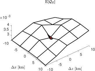
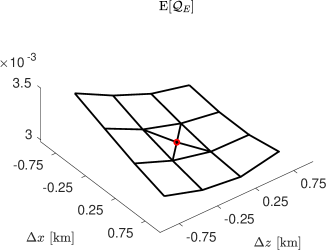
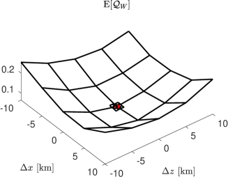
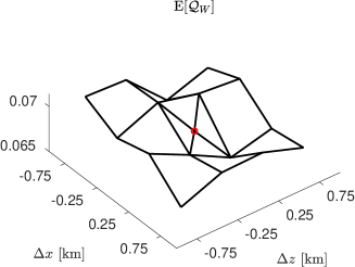
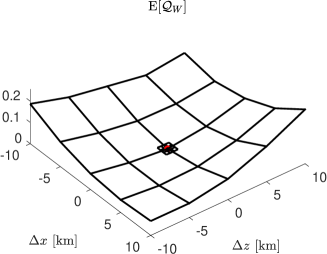
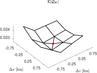
Figure 1: The expected value, ${\mathrm{E}\mspace{-2.0mu}\left[\mathcal{Q}(\mathbf{x_{s}^{~{}}},\bm{\theta})\right]}$, as a function of the shift between source location in the MLMC simulation and in the simulation used to generate the synthetic data; see Remark 2.
The top row shows $\mathcal{Q}_{E}$, computed with synthetic data with additive noise, the middle row $\mathcal{Q}_{W}$ with the same synthetic data, and the bottom row, $\mathcal{Q}_{W}$ without noise added to the synthetic data.
The effect of adding or removing a noise of this level is not visible in $\mathcal{Q}_{E}$, and therefore the corresponding figures of $\mathcal{Q}_{E}$ without added noise are omitted.

4 Computational Techniques

In this section, we start with a concise description of how Problem 1 and Problem 2 are approximated numerically. The domain, $D$, is modified in two steps: first, the finite Earth model is replaced by a half-plane in two dimensions or a half-space in three dimensions, and second, this semi-infinite domain is truncated, introducing absorbing boundary conditions on the artificial boundaries. We also describe a simplification of the stress tensor model (10) that results in a viscoelastic stress tensor suitable for numerical implementation. Then, we proceed with providing computational approximations of the QoI given in Section 3. The section ends with a summary of the MLMC algorithm for computing the expected value of the QoI.

4.1 Numerical Approximation of Initial Boundary Value Problem

A numerical approximation of Problem 1 or 2 can either be achieved by (i) approximating the seismic wave propagation produced by a seismic event on the whole Earth, or by (ii) restricting the computational domain, $D$, to a local region around the source and the receivers. In either case, there are purpose-built software packages based on the Spectral Element Method (SEM) [22, 24] that will be used in this paper. The MLMC method does not fundamentally depend on which of the alternatives, (i) or (ii), that is used, or on the choice of SEM over other approximation methods. Indeed, an important advantage of MLMC, or more generally MC, methods is that they are non-intrusive in the sense that they can straightforwardly be applied by randomly sampling the Earth material parameters and then executing any such publicly available simulation code to compute the corresponding sample of the QoI.

In our numerical example, we choose alternative (ii), and proceed in two steps: first, we approximate the Earth locally by a half-plane, in a two-dimensional test case, or by a half-space, in the full three-dimensional problem; second, the half-plane or half-space is truncated to a finite domain, where absorbing boundary conditions (ABC) are introduced on the artificial boundaries to mimic the absorption of seismic energy as the waves leave the region around the receivers. The variational equations (4) and (11) now contain a non-vanishing boundary term, corresponding to the part of the boundary, $\partial D_{A}$, where absorbing boundary conditions apply. We use a perfectly matched layer (PML) approximation of the ABC, introduced in [3] and used in many fields; see e.g. [38, 23] in the context of seismic wave propagation. However, in the absence of true PML, see [39], for Problem 2 which has attenuating Earth material properties, in practice we choose the truncation of $D$ such that $\partial D_{A}$ is far enough from all receivers to guarantee that no reflected waves reach the receivers in the time interval $[0,\mathcal{T}]$, given the maximal wave speeds allowed by the range of uncertainties (12).

To apply SEM, first, a semi-discrete version of the variational equation is introduced by discretizing space and introducing a finite dimensional solution space where the solution at time $t$ can be represented by a finite vector, $\mathbf{S}(t)$. Then, the time evolution of the SEM approximation, $\mathbf{S}(t)$, of the seismic wavefield solves an initial value problem for the second order ordinary differential equation (ODE) in time

$$M\ddot{\mathbf{S}}+C\dot{\mathbf{S}}+K\mathbf{S} =F, 0<t\leq\mathcal{T},$$ (24)

where $M$ is the mass matrix, $C$ is the global absorbing boundary matrix, $K$ the global stiffness matrix, and $F$ the source term.

To get the semi-discrete form, $D$ is divided into non-overlapping elements of maximal size $\Delta x$, similarly to what is done when using a standard finite-element method. Quadrilateral elements are used in two space dimensions and hexahedral in three. Each element is defined in terms of a number, $n_{c}$, of control points and an equal number of shape functions which describe the isomorphic mapping between the element and reference square or cube. The shape functions are products of Lagrange polynomials of low degree. In the remainder, we assume that no error is introduced by the representation of the shape of the elements, which is justified by the very simple geometry of the test problem in Section 5. The displacement field on every element is approximated by a Lagrange polynomial of higher degree, $N_{l}$, and the approximation of the variational form (4) or (11), including the artificial boundary term, over an element is based on the Gauss-Lobatto-Legendre integration rule on the same $N_{l}+1$ points used for Lagrange interpolation; this choice leads to a diagonal mass matrix, $M$, which is beneficial in the numerical stepping scheme. More details on the construction of these matrices and the source term can be found in [24].

The initial value problem for the ODE (24) is approximately solved by introducing a discretization of the time interval, and by applying a time-stepping method. Among multiple available choices, this work uses the second-order accurate explicit Newmark-type scheme; see for example Chapter 9 in [21]. It is a conditionally stable scheme and the associated condition on the time step leads to $\Delta t\leq c\,\Delta xN_{l}^{-2}$, for uniform spatial discretizations. Thanks to the diagonal nature of $M$ and the sparsity of $C$ and $K$, the cost per time step of the Newmark scheme is proportional to the number of unknowns in $\mathbf{S}(t_{j})$, and thus to $\Delta x^{-d}$, and since the number of time steps is inversely proportional to $\Delta t\propto\Delta x$ the total work is proportional to $\Delta x^{-(d+1)}$.

Determining $\Delta t$ by the stability constraint, $\Delta t\propto\Delta x$, we expect the second order accuracy of the Newmark scheme to asymptotically be the leading order error term as $\Delta x\to 0$, assuming sufficient regularity of the true solution.

4.2 Computational Model of Seismic Attenuation

Approximately solving Problem 2, as it is stated in Section 2.3, is very difficult since the stress $\mathbf{T}$ in (10) at time $t$ depends on the entire solution history $\mathbf{s}(\cdot,t^{\prime})$ for $-\infty<t^{\prime}\leq t$, or in practice for $0\leq t^{\prime}\leq t$ since the displacement is assumed to be constant up to time 0. Even in a discretized form in an explicit time stepping scheme, approximately updating the stress according to (10) would require storing the strain history for all previous time steps in every single discretization point where $\mathbf{T}$ must be approximated, requiring unfeasible amounts of computer memory and computational time. Therefore, the model of the viscoelastic properties of the medium is often simplified to a generalized Zener model using a series of “standard linear solid” (SLS) mechanisms. The present work uses the implementation of the generalized Zener model in SPECFEM2D. Below, we will briefly sketch the simplification of (10). For a more detailed description, we refer readers to [29, 42, 22, 31, 7].

The integral in the stress-strain relation (10) can be expressed as a convolution in time by defining the relaxation tensor $\mathbf{c}$ to be zero in $D\times\mathbb{R}^{-}$, i.e. $\mathbf{c}(\cdot,t)=\tilde{\mathbf{c}}(\cdot,t)H(t)$, where $H(t)$ is the Heaviside function. That is,

$$\mathbf{T}\left(\mathbf{x},t;\left\{\bm{\nabla}\mathbf{s}\right\}_{0}^{t}\right)=\int_{-\infty}^{\infty}\mathbf{c}(\mathbf{x},t-t^{{}^{\prime}})\mathbin{\vcentcolon}\partial_{t}\bm{\epsilon}(\bm{\nabla}\mathbf{s}(\mathbf{x},t^{{}^{\prime}}))\,dt^{{}^{\prime}}=\left(\mathbf{c}\ast\partial_{t}\bm{\epsilon}\right)(\mathbf{x},t)\\ =\left(\partial_{t}\mathbf{c}\ast\bm{\epsilon}\right)(\mathbf{x},t),$$ (25)

which, as discussed in [12], can be formulated in the frequency domain as

$$\widehat{}\mathbf{T}(\mathbf{x},\omega) =\widehat{\mathbf{M}}(\mathbf{x},\omega)\widehat{}\bm{\epsilon}(\mathbf{x},\omega),$$ (26)

where $\mathbf{M}(\cdot,t)=\partial_{t}\mathbf{c}(\cdot,t)$. In seismology, it has been observed, [8], that the so-called quality factor

$$Q(\omega) =\frac{Re\left(\widehat{\mathbf{M}}(\cdot,\omega)\right)}{Im\left(\widehat{\mathbf{M}}(\cdot,\omega)\right)},$$ (27)

is approximately constant over a wide range of frequencies. This $Q$ is an intrinsic property of the Earth material that describes the decay of amplitude in seismic waves due to the loss of energy to heat, and its impact on $\mathbf{M}$ is explicitly given in equation (5) of [12]. This observation allows modeling $\widehat{\mathbf{M}}(\cdot,\omega)$ in the frequency domain through a series of a number, $B$, of SLS. Then the stress-strain relation (25) can be approximated as

$$\mathbf{T} =\mathbf{c}^{U}\mathbin{\vcentcolon}\bm{\epsilon}-\sum_{b=1}^{B}\mathbf{R}^{b},$$ (28)

where $\mathbf{c}^{U}$ is the unrelaxed viscoelastic fourth order tensor, which for an isotropic Earth model is defined by $\lambda$ and $\mu$ or equivalently $\alpha$ and $\beta$. The relaxation functions $\mathbf{R}^{b}$ for each SLS satisfy initial value problems for a damping ODE; by the non-linear optimization approach given in [5], implemented in SPECFEM2D and used in this work, the ODE for each $\mathbf{R}^{b}$ is determined by two parameters: the quality factor, $Q$, and the number of SLS, $B$.

4.3 Quantities of Interest

The two QoI, $\mathcal{Q}_{E}$ and $\mathcal{Q}_{W}$ defined in (18) and (23) respectively, are approximated from discrete time series $\{\mathbf{s}(\mathbf{x}_{\mathbf{r}},t_{j}^{s};\cdot,\cdot)\}_{j=0}^{J}$ and $\{\mathbf{d}(\mathbf{x}_{\mathbf{r}},t_{k}^{d})\}_{k=0}^{K}$. The data observation times $0=t_{0}^{d}<\ldots<t_{K}^{d}=\mathcal{T}$, are considered given and fixed, and with realistic frequencies of the measurements, $100-200\,\mathrm{Hz}$, it is natural to take smaller time steps in the time discretization $0=t_{0}^{s}<\dots<t_{J}^{s}=\mathcal{T}$ of the numerical approximation of $\mathbf{s}$ and we assume that $\left\{t_{k}^{d}\right\}_{k=0}^{K}\subseteq\left\{t_{j}^{s}\right\}_{j=0}^{J}$. Furthermore, the time discretization is assumed to be characterized by one parameter $\Delta t$, e.g., the constant time step size of a uniform discretization. Since we defined both QoI as sums over all receivers and all components of the vector-valued functions $\mathbf{s}$ and $\mathbf{d}$ in the receivers, it is sufficient to describe the approximation in the case of two scalar functions $\phi^{s}$, representing the simulated displacement, and $\phi^{d}$, representing the observed data. Here, we define the function $\phi^{d}$ as the piecewise linear interpolation in time of the data points.

Approximation of $\mathcal{Q}_{E}$

The time integral in (18) is approximated by the Trapezoidal rule on the time discretization of the numerical simulation. With the assumption that $\{t_{k}^{d}\}_{k=0}^{K}\subseteq\{t_{j}^{s}\}_{j=0}^{J}$ and the definition of $\phi^{d}$ as the piecewise linear interpolation in time of the data points, only the discretization of $\phi^{s}$ contributes to the error. The numerical approximation of $\mathcal{Q}_{E}$ will then have an $\mathcal{O}(\Delta t^{2})$ asymptotic error, provided that $\phi^{s}$ is sufficiently smooth.

Approximation of $\mathcal{Q}_{W}$

The approximation of (23), through (22), requires both positive and negative values to be attained in all components of $\{\mathbf{s}(\mathbf{x}_{\mathbf{r}},t_{j}^{s};\cdot,\cdot)\}_{j=0}^{J}$ and $\{\mathbf{d}(\mathbf{x}_{\mathbf{r}},t_{k}^{d})\}_{k=0}^{K}$ in all receivers; see Remark 1 on page 1. Assuming that this holds we approximate the $W_{2}^{2}$-distance between the normalized non-negative parts of $\phi^{s}$ and $\phi^{d}$; we treat the non-positive analogously. To this end, the zeros of $\phi^{s}$ and $\phi^{d}$, denoted $\{z_{j}^{s}\}_{j=0}^{\hat{J}}$ and $\{z_{k}^{d}\}_{k=0}^{\hat{K}}$ respectively, are approximated by linear interpolation, and they are included in the respective time discretizations, generating $\{t_{j}^{s}\}_{j=0}^{J^{\ast}}=\{t_{j}^{s}\}_{j=0}^{J}\bigcup\{z_{j}^{s}\}_{j=0}^{\hat{J}}$ and $\{t_{k}^{d}\}_{k=0}^{K^{\ast}}=\{t_{k}^{d}\}_{k=0}^{K}\bigcup\{z_{k}^{d}\}_{k=0}^{\hat{K}}$, and thus $\{\phi_{j}^{s,+}\}_{j=0}^{J^{\ast}}$ and $\{\phi_{k}^{d,+}\}_{k=0}^{K^{\ast}}$ are obtained. Then the corresponding values of the CDFs, $\{\Phi_{j}^{s,+}\}_{j=0}^{J^{\ast}}$ and $\{\Phi_{k}^{d,+}\}_{k=0}^{K^{\ast}}$ are approximated by the Trapezoidal rule, followed by normalization. Finally, the inverse of $\Phi^{d,+}$ in $\{\Phi_{j}^{s,+}\}_{j=0}^{J^{\ast}}$, i.e. $\left\{\left[\Phi^{d,+}\right]^{-1}\left(\Phi_{j}^{s,+}\right)\right\}_{j=0}^{J^{\ast}}$, is approximated by linear interpolation, and analogously for the inverse of $\Phi^{s,+}$ in $\{\Phi_{k}^{d,+}\}_{k=0}^{K^{\ast}}$, before the integral in (21) is approximated by the Trapezoidal rule on the discretization $\{\Phi_{j}^{s,+}\}_{j=0}^{J^{\ast}}\bigcup\{\Phi_{k}^{d,+}\}_{k=0}^{K^{\ast}}$ of $[0,1]$. These steps combined lead to an $\mathcal{O}(\Delta t^{2})$ asymptotic error, provided that $\phi^{s}$ is sufficiently smooth.

Remark 3 (Cost of approximating $\mathcal{Q}_{W}$).

In the present context, passive source-inversion with a small number of receivers, in the order of 10, the cost of approximating $\mathcal{Q}_{W}$ from $\mathbf{s}$ and $\mathbf{d}$ is negligible compared to that of computing the approximation of $\mathbf{s}$ itself. This might not always be the case in other contexts where one has data from a large number of receivers, as could be the case e.g. in seismic imaging for oil and gas exploration.

Remark 4 (On expected weak and strong convergence rates).

The deterministic rate of convergence, as $\Delta t^{s}\to 0$, of both $\mathcal{Q}$ approximations, is two. Here, $\Delta t^{s}$ is identical to the time step of the underlying approximation method of Problem 1 or 2. In the numerical approximation of $\mathbf{s}$, with the second order Newmark scheme in time, the asymptotic convergence rate is also two at best, which holds if the solution is sufficiently regular. By our assumptions on the random fields satisfying the same regularity as in the deterministic case and being uniformly bounded, from above and away from zero from below, in the physical domain and with respect to random outcomes, we expect both the weak and the strong rates of convergence to be the same as the deterministic convergence rate of the numerical approximation; i.e. at best two, asymptotically as $\Delta t\propto\Delta x$ goes to zero.

4.4 MLMC Algorithm

Here, we summarize the MLMC algorithm introduced by Giles [16] and independently, in a setting further from the one used here, by Heinrich in [19], which has since become widely used [17].

MLMC is a way of reducing the computational cost of standard MC, for achieving a given accuracy in the estimation of the expected value of some QoI, in situations when the samples in the MC method are obtained by numerical approximation methods characterized by a refinement parameter, $h_{\ell}$, controlling both the accuracy and the cost.

Goal

We aim to approximate the expected value of some QoI, ${\mathrm{E}\mspace{-2.0mu}\left[\mathcal{Q}\right]}$, by an estimator $\mathcal{A}$, with the accuracy requirement that

$$|{\mathrm{E}\mspace{-2.0mu}\left[\mathcal{Q}\right]}-\mathcal{A}| \leq\mathrm{TOL}, 1-\xi 0<\xi\ll 1$$ with probability , for , (29)

where $\mathrm{TOL}>0$ is a user-prescribed error tolerance. To this end we require

$$\left|{\mathrm{E}\mspace{-2.0mu}\left[\mathcal{Q}-\mathcal{A}\right]}\right| \leq(1-\varphi)\mathrm{TOL}$$ (30a)

and

$${\mathrm{P}\mspace{-2.0mu}\left[\left|{\mathrm{E}\mspace{-2.0mu}\left[\mathcal{A}\right]}-\mathcal{A}\right|>\varphi\mathrm{TOL}\right]} \leq\xi,$$ (30b)

for some $0<\varphi<1$, which we are free to choose.

Assumptions on the Numerical Approximation Model

Consider a sequence of discretization-based approximations of $\mathcal{Q}$ characterized by a refinement parameter, $\{h_{\ell}\}_{\ell=0}^{\infty}$. Let $\mathcal{Q}_{\ell}(\bm{\theta})$ denote the resulting approximation of $\mathcal{Q}$, using the refinement parameter $h_{\ell}$ for an outcome of the random variable $\bm{\theta}$. In this work, we consider successive halvings in the refinement parameter, $h_{\ell}=2^{-\ell}$, which in Section 4.1 corresponds to the spatial mesh size and the temporal step size, $\Delta x_{\ell}=\Delta x_{0}h_{\ell}$ and $\Delta t_{\ell}=\Delta t_{0}h_{\ell}$, respectively. We then make the following assumptions on how the cost and accuracy of the numerical approximations depend on $h_{\ell}$. We assume that the work per sample of $\mathcal{Q}_{\ell}$, denoted $W_{\ell}$, depends on $h_{\ell}$ as

$$W_{\ell} \propto h_{\ell}^{-\gamma}, \gamma>0,$$ (31a)

and the weak order of convergence is $${q_{w}}$$, so that we can model,

$$|{\mathrm{E}\mspace{-2.0mu}\left[\mathcal{Q}-\mathcal{Q}_{\ell}\right]}| ={K_{w}}h_{\ell}^{q_{w}}, {K_{w}},{q_{w}}>0,$$ (31b)

and that the variance is independent of the refinement level

$${\mathrm{Var}\mspace{-2.0mu}\left[\mathcal{Q}_{\ell}\right]} ={V_{0}}, {V_{0}}>0.$$ (31c)

Standard MC estimator

For $N$ i.i.d. realizations of the parameter, $\{\bm{\theta}_{n}\}_{n=1}^{N}$, the unbiased MC estimator of ${\mathrm{E}\mspace{-2.0mu}\left[\mathcal{Q}_{\ell}(\bm{\theta})\right]}$ is given by

$$\mathcal{A}_{MC} =\frac{1}{N}\sum_{n=1}^{N}\mathcal{Q}_{\ell}(\bm{\theta}_{n}).$$ (32)

For $\mathcal{A}_{MC}$ to satisfy (30) we require

$$\left|{\mathrm{E}\mspace{-2.0mu}\left[\mathcal{Q}-\mathcal{Q}_{\ell}\right]}\right| \leq(1-\varphi)\mathrm{TOL},$$ (33)

which according to the model (31b) becomes

$${K_{w}}h_{\ell}^{q_{w}} \leq(1-\varphi)\mathrm{TOL}.$$ (34)

For any fixed $h_{\ell}$ such that ${K_{w}}h_{\ell}^{q_{w}}<\mathrm{TOL}$, the value of the splitting parameter, $\varphi$, is implied by replacing the inequality in (34) by equality and solving for $\varphi$, giving

$$\varphi =1-\frac{{K_{w}}h_{\ell}^{q_{w}}}{\mathrm{TOL}}.$$ (35)

Thus, the model for the bias tells us how large of a statistical error we can afford for the desired tolerance, $\mathrm{TOL}$. By the Central Limit Theorem, $\mathcal{A}_{MC}$ properly rescaled converges in distribution,

$$\frac{\sqrt{N}\left({\mathrm{E}\mspace{-2.0mu}\left[\mathcal{Q}_{\ell}\right]}-\mathcal{A}_{MC}\right)}{\sqrt{{V_{0}}}} \Rightarrow\mathcal{N}(0,1), \text{as $N\to\infty$},$$ (36)

where $\mathcal{N}(0,1)$ is a standard normal random variable with CDF $\Phi_{\mathcal{N}(0,1)}$. Hence, to satisfy the statistical error constraint (30b), asymptotically as $\mathrm{TOL}\to 0$, we require

$$\frac{{V_{0}}}{N} \leq\left(\frac{\varphi\mathrm{TOL}}{C_{\xi}}\right)^{2},$$ (37)

where $C_{\xi}$ is the confidence parameter corresponding to a $1-\xi$ confidence interval, i.e. $\Phi_{\mathcal{N}(0,1)}(C_{\xi})=1-\xi/2$.

The computational work of generating $\mathcal{A}_{MC}$ is

$$W_{\mathrm{MC}} \propto NW_{\ell}.$$

For asymptotic analysis, assume that we can choose $h_{\ell}$ by taking equality in (34) and $N$ by taking equality in (37); then we get the asymptotic work estimate

$$W_{\mathrm{MC}} \propto\frac{\mathrm{TOL}^{-\left(2+\gamma/{q_{w}}\right)}}{\varphi^{2}\left(1-\varphi\right)^{\gamma/{q_{w}}}}.$$ (38)

For any fixed choice of $\varphi$, the computational complexity of the MC method is $\mathrm{TOL}^{-\left(2+\gamma/{q_{w}}\right)}$. Minimizing the right hand side in (38) with respect to $\varphi$ gives the asymptotically optimal choice

$$\varphi =\left(1+\frac{\gamma}{2{q_{w}}}\right)^{-1}\in(0,1).$$ (39)

MLMC estimator

The work required to meet a given accuracy by standard MC can be significantly improved by systematic generation of control variates given by approximations corresponding to different mesh sizes. In the standard MLMC approach, we use a whole hierarchy of $L+1$ meshes defined by decreasing mesh sizes $\{h_{\ell}\}_{\ell=0}^{L}$ and the telescoping representation of the expected value of the finest approximation, $\mathcal{Q}_{L}$,

$${\mathrm{E}\mspace{-2.0mu}\left[\mathcal{Q}_{L}\right]} ={\mathrm{E}\mspace{-2.0mu}\left[\mathcal{Q}_{0}\right]}+\sum_{\ell=1}^{L}{\mathrm{E}\mspace{-2.0mu}\left[\mathcal{Q}_{\ell}-\mathcal{Q}_{\ell-1}\right]},$$

from which the MLMC estimator is obtained by approximating the expected values in the telescoping sum by sample averages as

$$\mathcal{A}_{MLMC} =\frac{1}{N_{0}}\sum_{n=1}^{N_{0}}\mathcal{Q}_{0}(\bm{\theta}_{0,n})+\sum_{\ell=1}^{L}\frac{1}{N_{\ell}}\sum_{n=1}^{N_{\ell}}\left(\mathcal{Q}_{\ell}(\bm{\theta}_{\ell,n})-\mathcal{Q}_{\ell-1}(\bm{\theta}_{\ell,n})\right),$$ (40)

where $\{\bm{\theta}_{\ell,n}\}_{n=1,\dots,N_{\ell}}^{\ell=0,\dots,L}$ denote i.i.d. realizations of the mesh-independent random variables. Note that the correction terms

$$\Delta\mathcal{Q}_{\ell}(\bm{\theta}_{\ell,n}) =\mathcal{Q}_{\ell}(\bm{\theta}_{\ell,n})-\mathcal{Q}_{\ell-1}(\bm{\theta}_{\ell,n})$$ (41)

are evaluated with the same outcome of $\bm{\theta}_{\ell,n}$ in both the coarse and the fine mesh approximation. This means that ${\mathrm{Var}\mspace{-2.0mu}\left[\Delta\mathcal{Q}_{\ell}\right]}\to 0$, as $\ell\to\infty$, provided that the numerical approximation $\mathcal{Q}_{\ell}$ converges strongly. Introducing the notation

$$V_{\ell} =\begin{cases}{\mathrm{Var}\mspace{-2.0mu}\left[\mathcal{Q}_{0}\right]},&\ell=0,\\ {\mathrm{Var}\mspace{-2.0mu}\left[\mathcal{Q}_{\ell}-\mathcal{Q}_{\ell-1}\right]},&\ell>0,\end{cases}$$ (42)

and assuming a strong convergence rate ${q_{s}}/2$ we model

$$V_{\ell} ={K_{s}}h_{\ell}^{{q_{s}}}, \text{ for }\ell>0.$$ (43)

Note that while this holds asymptotically as $\ell\to\infty$, by the definition of strong convergence, this model may be inaccurate for small $\ell$, corresponding to coarse discretizations. However, it suffices for an asymptotic work estimate.

The computational work needed to generate $\mathcal{A}_{MLMC}$ is

$$W_{\mathrm{MLMC}} =\sum_{\ell=0}^{L}N_{\ell}W_{\ell},$$ (44)

where we now assume that (31a) also holds for the cost of generating $\Delta\mathcal{Q}_{\ell}$. In order for $\mathcal{A}_{MLMC}$ to satisfy (29), we fix $\varphi\in(0,1)$ and require $\mathcal{A}_{MLMC}$ to satisfy the bias constraint (33) and, consequently (34), on the finest discretization, $\ell=L$, leading to

$$h_{L} =\left(\frac{(1-\varphi)\mathrm{TOL}}{{K_{w}}}\right)^{1/{q_{w}}},$$ (45)

and we also require it to satisfy the statistical error constraint (30b). In the MLMC context, (30b) is approximated by the bound

$$\sum_{\ell=0}^{L}\frac{V_{\ell}}{N_{\ell}} \leq\left(\frac{\varphi\mathrm{TOL}}{C_{\xi}}\right)^{2}$$ (46)

on the variance of $\mathcal{A}_{MLMC}$. Enforcing (30b) through this bound is justified asymptotically, as $\mathrm{TOL}$ converges to 0, by a Central Limit Theorem for MLMC estimators if for example ${q_{s}}>\gamma$; see Theorem 1.1 in [20]. Given $L$ and $\varphi$, minimizing the work (44) subject to the constraint (46) leads to the optimal number of samples per level in $\mathcal{A}_{MLMC}$,

$$N_{\ell} =\left(\frac{C_{\xi}}{\varphi\mathrm{TOL}}\right)^{2}\sqrt{\frac{V_{\ell}}{W_{\ell}}}\sum_{\ell=0}^{L}\sqrt{W_{\ell}V_{\ell}}.$$ (47)

Substituting this optimal $N_{\ell}$ in the total work (44) yields:

$$W_{\mathrm{MLMC}} =\left(\frac{C_{\xi}}{\varphi\mathrm{TOL}}\right)^{2}\left(\sum_{\ell=0}^{L}\sqrt{W_{\ell}V_{\ell}}\right)^{2}.$$ (48)

Finally, using the mesh parameter given by (45), work per sample (31a), and for simplicity assuming that (43) also holds for $\ell=0$, this computational work has the asymptotic behavior

$$W_{\mathrm{MLMC}} \propto\begin{cases}\mathrm{TOL}^{-2},&\text{if ${q_{s}}>\gamma$},\\ \mathrm{TOL}^{-2}\left(\log{\mathrm{TOL}^{-1}}\right)^{2},&\text{if ${q_{s}}=\gamma$},\\ \mathrm{TOL}^{-2\left(1+\frac{\gamma-{q_{s}}}{2{q_{w}}}\right)},&\text{if ${q_{s}}<\gamma$},\end{cases}$$ (49)

as $\mathrm{TOL}\to 0$, assuming ${q_{w}}\geq\min{\left({q_{s}},\gamma\right)}/2$; see e.g. Theorem 3.1 in [16], or Corollary 2.1 and Corollary 2.2 in [18]. Similar to the standard MC case, it is possible to optimize the choice of $\varphi$ in (30) for MLMC. In particular, if ${q_{s}}>\gamma$, an asymptotic analysis gives $\varphi\to 1$, as $\mathrm{TOL}\to 0$, indicating an aggressive refinement of the numerical discretization to reduce the bias. Again, the choice of $\varphi$ does not change the rate of the complexity, but an optimal choice may reduce the work with a constant factor.

In all three cases in (49), the complexity is lower than the corresponding complexity, $\mathrm{TOL}^{-\left(2+\gamma/{q_{w}}\right)}$, for standard MC simulation of the same problem (38). This leads to very significant computational saving in complex models, and as a result some problems that are infeasable using the standard MC method are computationally tractable using MLMC.

MLMC applied to ${\mathrm{E}\mspace{-2.0mu}\left[\mathcal{Q}_{\ell}\right]}$ of Section 4.1–4.3

The assumption on the work per sample (31a) holds for $\gamma=d+1$, since the degrees of freedom in the uniform spatial discretization are proportional to $h_{\ell}^{-d}$, and the number of time steps is proportional to $h_{\ell}^{-1}$, where work per time step of the explicit time stepping scheme is proportional to the degrees of freedom. In the setting described in Section 2–3, the weak convergence rate, ${q_{w}}$, is identical to the rate of convergence in the approximation of the deterministic problem, and the strong convergence rate, ${q_{s}}/2$, equals the weak rate. The explicit Newmark time stepping scheme and the numerical approximation of $\mathcal{Q}_{E}$ and $\mathcal{Q}_{W}$ are both of order 2, so that asymptotically as $h_{\ell}\to 0$ we expect ${q_{w}}=2$ and ${q_{s}}=4$ assuming sufficiently regular exact solution. Based on these observations, summarized in Table 1, and the complexity estimates (38) and (49), we expect the asymptotic complexity to improve from $\mathrm{TOL}^{-3.5}$ to $\mathrm{TOL}^{-2}$, for $d=2$, and from $\mathrm{TOL}^{-4}$ to $\mathrm{TOL}^{-2}(\log{(\mathrm{TOL}^{-1})})^{2}$, for $d=3$, as $\mathrm{TOL}\to 0$ and standard MC is replaced by MLMC.

	Model parameters			Asymptotic complexity
$d$	$\gamma$	${q_{w}}$	${q_{s}}$	$W_{\mathrm{MC}}$	$W_{\mathrm{MLMC}}$
2	3	2	4	$\mathrm{TOL}^{-3.5}$	$\mathrm{TOL}^{-2}$
3	4			$\mathrm{TOL}^{-4}$	$\mathrm{TOL}^{-2}(\log{(\mathrm{TOL}^{-1})})^{2}$

Table 1: Summary of the parameters in the work and convergence models (31) and (43), for the numerical approximation of Problem 1 or Problem 2, given in Section 4.1–4.3, and the corresponding asymptotic complexity estimates, given in (38) and (49).

5 Numerical Tests

These numerical experiments make up an initial study of the validity of MLMC techniques as a means of accelerating the approximation of expected values of source inversion misfit functions, where we take the expectation with respect to random parameters modeling uncertainties in the Earth model. After this initial study where the source is approximated to a point and only synthetic data are used, our ultimate goal is to integrate MLMC into the full source inversion problem where the finite fault solution is to be inferred by using real seismological data. While the final source inversion must be based on numerical simulations on a three-dimensional Earth model, these initial tests were made on a two-dimensional model described in the following. Furthermore, the misfit functions were chosen with the aim of identifying the source location considering the source moment tensor as fixed.

We first describe the problem setup, including the source model, computational geometry, discretization, random Earth material parameters, and the synthetic data replacing actual measurements in the two-dimensional test. Finally, we describe the execution and results of MLMC computations on the given problem setup.

5.1 Problem Setup

For the numerical tests with $d=2$, we create a geometry consistent with an actual network of receivers, belonging to a small seismic network in the Ngorongoro Conservation Area on the East Rift, in Tanzania. We do this by selecting three receivers that are approximately aligned with the estimated epicenter of a seismic event that was recorded. Figure 2 illustrates the physical configuration. The rough alignment of the source and the receiver locations in the actual seismic network make this event a good opportunity to run the tests in a two-dimensional domain. We describe the two-dimensional computational domains below, together with the source and Earth parameters.

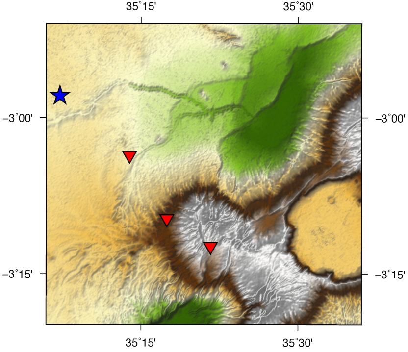
Figure 2: Source–receivers–geometry for the Tanzania case study, restricted to three receivers, marked by red triangles, which fall approximately along a straight line, also aligned with the estimated source location of a recorded seismic event (marked by a blue star).

5.1.1 Source model

We consider a point source with a symmetric moment tensor, modeled as a body force in the variational equation (11) of Problem 2,

$$\int_{D}\mathbf{f}(\mathbf{x},t)\cdot\mathbf{w}(\mathbf{x})\,d\mathbf{x} =-\mathbf{M}\mathbin{\vcentcolon}\bm{\nabla}\mathbf{w}(\mathbf{x_{s}^{~{}}})S(t),$$

with the moment tensor

$$\mathbf{M} =\left(\begin{array}[]{cc}5.5895\cdot 10^{13}&7.9762\cdot 10^{13}\\ 7.9762\cdot 10^{13}&-2.5698\cdot 10^{14}\end{array}\right),$$

measured in $\mathrm{Nm}$, and a Gaussian source-time function with corner frequency $f_{0}=2\,\mathrm{Hz}$,

$$S(t) =\dfrac{3f_{0}}{\sqrt{2\pi}}\exp\left(-\frac{9f_{0}^{2}(t-t_{c})^{2}}{2}\right).$$

The time source function is centered at time $t_{c}=0\,\mathrm{s}$; the solution time interval starts at $t_{0}=-0.6\,\mathrm{s}$ and ends at $\mathcal{T}=25\,\mathrm{s}$, and the QoI is based on $0\leq t\leq\mathcal{T}$.

5.1.2 Computational Domain

The heterogeneous Earth is initially modeled with six homogeneous layers of variable thickness, as stated in Table 2, and terminated by an infinite half-space. The layers are separated by horizontal interfaces; topography is not included here. The source-receiver geometry is defined by the depth (vertical distance from the free surface) of the point source and the horizontal distances between the point source and the three receivers, as given in Table 3 and shown in Figure 3.

As described in Section 4.1, the half-plane domain is approximated by a finite domain, with absorbing boundary conditions on the three artificial boundaries. In the numerical approximation of Problem 2 with seismic attenuation, the PML boundary conditions are not perfectly absorbing, but reflections are created at the boundary; see e.g. Section 3.4 in [25]. The finite domain is defined by three additional parameters $x_{s}$, $\Delta D_{x}$, and $\Delta D_{z}$, which are chosen large enough so that no reflections reach any of the three receivers during the simulation time interval, $[-0.6,\mathcal{T}]\,\mathrm{s}$, given the maximal velocities in the ranges of uncertainties.

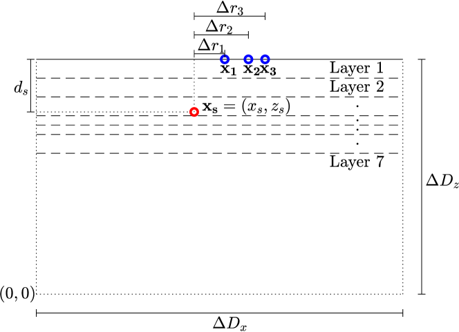
Figure 3: Domain of the two-dimensional model. Four parameters define the configuration: the depth of the source, $d_{s}>0$, and the signed horizontal distances between the source and the three receivers, $\Delta r_{1},\Delta r_{2},\,\mathrm{and}\,\Delta r_{3}$. The horizontal coordinate direction is denoted $x$ and the vertical $z$.

Layer	Thickness
1	10 $\mathrm{km}$
2	10 $\mathrm{km}$
3	10 $\mathrm{km}$
4	5 $\mathrm{km}$
5	5 $\mathrm{km}$
6	10 $\mathrm{km}$
7	–

Table 2: Thickness of the layers in the half-plane two dimensional Earth model.

	Synthetic Data	MLMC
$d_{s}$	$28.000\,\mathrm{km}$	$28.000\,\mathrm{km}$
$\Delta r_{1}$	$16.242\,\mathrm{km}$	$11.242\,\mathrm{km}$
$\Delta r_{2}$	$28.849\,\mathrm{km}$	$23.849\,\mathrm{km}$
$\Delta r_{3}$	$37.724\,\mathrm{km}$	$32.724\,\mathrm{km}$
$x_{s}$	$84.000\,\mathrm{km}$	$86.500\,\mathrm{km}$
$\Delta D_{x}$	$195.000\,\mathrm{km}$	$195.000\,\mathrm{km}$
$\Delta D_{z}$	$125.000\,\mathrm{km}$	$125.000\,\mathrm{km}$

Table 3: Parameters defining the configuration in the half-plane geometry, $d_{s}$, $\Delta r_{1}$, $\Delta r_{2}$, and $\Delta r_{3}$, and additional parameters defining the truncated numerical domain, $x_{s}$, $\Delta D_{x}$, and $\Delta D_{z}$. See Figure 3.

Discretization of the computational domain

For the numerical computations using SPECFEM2D version $7.0$ [25] in double precision, the computational domain is discretized uniformly into squares of side $\Delta x_{\ell}$, with the coarsest mesh using $\Delta x_{0}=2500\,\mathrm{m}$ so that the interfaces always coincide with element boundaries. These computations are based on spectral elements in two dimensions, using $n_{c}=9$ control points to define the isomorphism between the computational element and the reference element, a basis of Lagrange polynomials of degree $N_{l}=4$, and $5\times 5$ Gauss-Lobatto-Legendre quadrature points. The second order Newmark explicit time stepping scheme was used with step size $\Delta t_{0}=6.25\cdot 10^{-3}\,\mathrm{s}$ on the coarsest discretization, which was refined at the same rate as $\Delta x_{\ell}$ to keep the approximate CFL condition satisfied. A PML consisting of three elements was used on the artificial boundaries.

5.1.3 Earth material properties

The viscoelastic property of the Earth material, as described in Section 4.2, is approximated by a generalized Zener model, implemented in SPECFEM2D, with $B=3$ SLS and the quality factor, $Q$, which is constant in each layer (Table 4). The quality factor is kept constant throughout the simulations.

As described in Section 2, the triplet $(\rho,\alpha,\beta)$, denoting the density, compression wave speed, and shear wave speed, respectively, defines the Earth’s material properties with varying spatial position. In the particular seven-layer domain introduced above, a one-dimensional, piecewise constant velocity model is used. These three fields are then completely described by three seven-dimensional random variables, $\bm{\alpha}$, $\bm{\beta}$, and $\bm{\rho}$. Here, we detail the probability distributions we assign to these parameters. To prepare the inversion of real data, $\alpha$, $\beta$, and $\rho$ are adapted from the results of [2] and [35] obtained from previous seismological experiments in adjacent areas. Among the unperturbed values, denoted with a bar over the symbols, listed in Table 4, $\bar{\bm{\beta}}$ and $\bar{\bm{\rho}}$ are treated as primary parameters, while $\bm{\bar{\alpha}}$ is scaled from $\bar{\bm{\beta}}$. The relation

$$\nu =\dfrac{\bar{\alpha}_{i}}{\bar{\beta}_{i}}=1.7, i=1,2,\dots,7,$$ (50)

is chosen because it is a common use for crustal structure and it is in agreement with previous seismological studies in the area [35].

layer, $i$	$\bar{\rho}_{i}$	$\bar{\beta}_{i}$	$\bar{\alpha}_{i}$	$Q$
1	$2500$	$3529.0$	$6034.6$	$300$
2	$2500$	$3705.0$	$6335.6$	$300$
3	$2500$	$3882.0$	$6638.2$	$800$
4	$2500$	$3911.0$	$6687.8$	$800$
5	$2900$	$4422.7$	$7562.8$	$800$
6	$2900$	$4506.4$	$7705.9$	$600$
7	$2900$	$4533.6$	$7752.5$	$600$

Table 4: Unperturbed values of the material parameters. Here $\bar{}\rho$, $\bar{\beta}$, and $\bar{\alpha}$ are given in the units $\mathrm{kg}/\mathrm{m}^{3}$, $\mathrm{m}/\mathrm{s}$, and $\mathrm{m}/\mathrm{s}$, respectively. The quality factor, $Q$, used in the seismic attenuation model is dimensionless and kept unperturbed in all simulations.

We model the uncertain shear wave speed, $\bm{\beta}$, as a uniformly distributed random variable

$$\boldsymbol{\beta} \sim\bm{\mathcal{U}}\left(\prod_{i=1}^{7}[\beta_{i}^{lb},\beta_{i}^{ub}]\right),$$

with independent components, and where the range is a plus-minus 10% interval around the unperturbed value, i.e.

$$\beta_{i}^{lb} =(1-q)\cdot\bar{\beta}_{i}, \beta_{i}^{ub} =(1+q)\cdot\bar{\beta}_{i}, i=1,2,\dots,7,$$

where $q=0.1$. In keeping with (50), but assuming some variability in the ratio, the compressional wave speed, $\bm{\alpha}$, is modeled by a random variable which, conditioned on $\bm{\beta}$, is uniformly distributed with independent components,

$$\bm{\alpha} \sim\bm{\mathcal{U}}\left(\prod_{i=1}^{7}[\nu^{lb}\cdot\beta_{i},\nu^{ub}\cdot\beta_{i}]\right),$$

where $\nu^{lb}=1.64$ and $\nu^{ub}=1.78$, corresponding to a range of variability of about $\pm 4\%$. Finally, the density, $\bm{\rho}$, is again uniformly distributed with independent components

$$\bm{\rho} \sim\bm{\mathcal{U}}\left(\prod_{i=1}^{7}[\rho_{i}^{lb},\rho_{i}^{ub}]\right),$$

where

$$\rho_{i}^{lb} =(1-r)\bar{\rho}_{i}, \rho_{i}^{ub} =(1+r)\bar{\rho}_{i}, i=1,2,\dots,7,$$

with $r=0.1$.

Figure 4 shows the sample mean and contour lines of the sample CDF for these random parameters, based on samples used in the verification run of the problem setup.

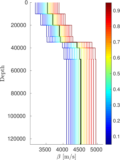
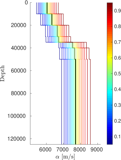
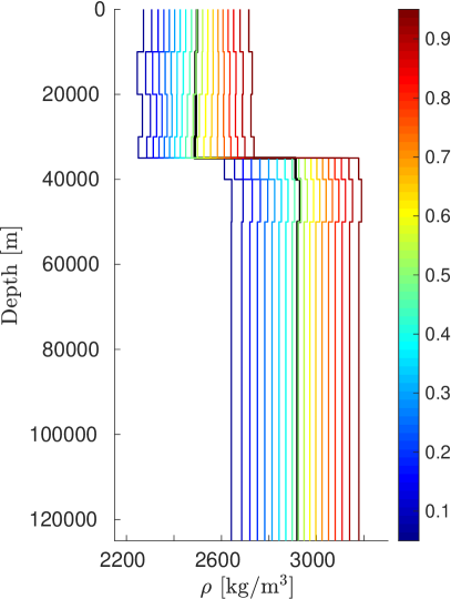
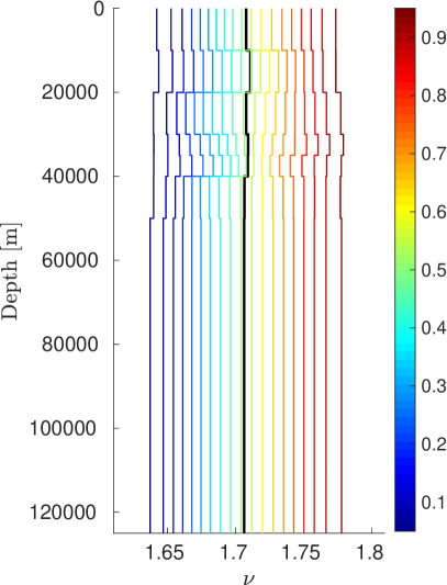
Figure 4: Sample average, marked with the thick black graph, and equidistributed quantiles, color-coded thinner graphs, of the Earth material parameters based on the 320 samples from the verification run.
(Top Left) Shear wave speed, $\beta$, (Top Right) Compressional wave speed, $\alpha$, (Bottom Left) Density, $\rho$, and (Bottom Right) $\nu=\alpha/\beta$.

5.1.4 Synthetic Data

Instead of actual, measured data from seismic activity, the misfit functions for the QoI in the two-dimensional computations use synthetic data obtained from the same underlying code using a finer discretization, $\Delta x=78.125\,\mathrm{m}$ and $\Delta t=1.953125\cdot 10^{-4}\,\mathrm{s}$, than any of the samples in the MLMC run. The source location relative to the receivers, listed in Table 3, agrees with the independently estimated epicenter in Figure 2 and the fixed Earth material parameters, listed in Table 5, correspond to one outcome of the sampling procedure in Section 5.1.3. The computed displacements are illustrated in the left column of Figure 5.

The resulting time series for the displacement in the three receivers are then restricted to a much coarser time discretization, corresponding to a frequency of measurements of $160\,\mathrm{Hz}$, that are in the realistic range of frequencies for measured seismograms, and i.i.d. noise $\bm{\varepsilon}_{k,n}\sim\mathcal{N}(\mathbf{0},\sigma^{2}\mathbf{I})$ with $\sigma=2.5\cdot 10^{-3}\approx 1\%$ of $\max{\mathbf{s}}$, is added as in (15); see the right column of Figure 5.

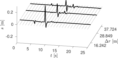
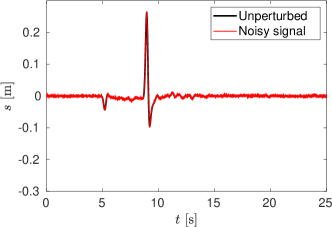
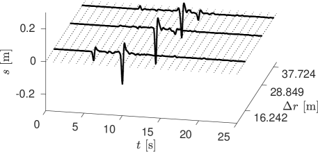
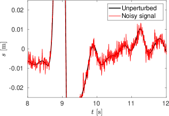
Figure 5: Synthetic data $\mathbf{d}(\mathbf{x}_{n},t)=\mathbf{s}(\mathbf{x}_{n},t;\mathbf{x_{s}^{\ast}},\bm{\theta}^{\ast})$, where the displacement $\mathbf{s}(\mathbf{x}_{n},t;\mathbf{x_{s}^{\ast}},\bm{\theta}^{\ast})$ is obtained from a computation with the source location, $\mathbf{x_{s}^{\ast}}$, and the geometry parameters of Figure 3 given in Table 3 and with a fixed outcome of the random Earth parameters, $\bm{\theta}^{\ast}$, within their ranges of uncertainty, as given in Table 5. To the left are the $x$-component (top) and $z$-component (bottom) of the synthetic data without added noise. To the right, the $x$-component in receiver location 1 is shown both with and without added noise, with the bottom being a detailed view of the top.

layer, $i$	$\rho_{i}$	$\beta_{i}$	$\alpha_{i}$
1	$2439.9$	$3498.0$	$5737.7$
2	$2715.8$	$3654.9$	$6346.0$
3	$2747.1$	$3690.9$	$6568.5$
4	$2562.0$	$4045.0$	$7038.2$
5	$2862.8$	$4491.8$	$7647.2$
6	$2862.0$	$4691.5$	$7753.4$
7	$2809.7$	$4969.8$	$8790.9$

Table 5: Values of the material parameters in the simulation which generated the synthetic data. Here $\rho$, $\beta$, and $\alpha$ are given in the units $\mathrm{kg}/\mathrm{m}^{3}$, $\mathrm{m}/\mathrm{s}$, and $\mathrm{m}/\mathrm{s}$, respectively, and rounded to five digits.

layer, $i$	$\rho_{i}$	$\beta_{i}$	$\alpha_{i}$
1	$2333.8$	$3789.8$	$6503.4$
2	$2539.0$	$3562.3$	$6117.5$
3	$2416.8$	$3726.8$	$6157.8$
4	$2521.5$	$3724.4$	$6176.2$
5	$2793.1$	$4062.9$	$7228.6$
6	$2822.0$	$4422.7$	$7602.2$
7	$2811.9$	$4612.2$	$7733.8$

Table 6: Values of the material parameters in the simulations used to assess the effect of including attenuation in the model. Units and rounding of $\rho$, $\beta$, and $\alpha$ as in Table 5.
 

5.1.5 The impact of attenuation on the QoIs

To assess the effect of attenuation in the problem described above, we compute the QoIs obtained with and without attenuation in the model, for one outcome of the Earth material parameters, given in Table 6, and with the geometry of the MLMC runs in Table 3, using discretization levels 1 and 2 in Table 8. Including attenuation changed both QoIs several percent; see Table 7.

The significantly reduced computing time of MLMC, compared to standard MC with corresponding accuracy, allows for simulation with an error tolerance small enough to evaluate the usefulness of including attenuation in the model in the presence of uncertainty in the Earth material parameters.

An alternative variant of the MLMC approach in this paper, would be to use QoIs sampled using the elastic model as control variates for QoIs sampled using the model with attenuation. Since the work associated with the elastic model is smaller, we expect an MLMC method where coarse grid samples are based on the elastic model to further reduce the computational cost of achieving a desired accuracy in the expected value of the QoI.

	Level, $\ell$	Elast.	Atten.	Change
$\mathcal{Q}_{E}$	1	4.20$\cdot 10^{-3}$	3.82$\cdot 10^{-3}$	-9.1%
	2	4.24$\cdot 10^{-3}$	3.85$\cdot 10^{-3}$	-9.2%
$\mathcal{Q}_{W}$	1	8.94$\cdot 10^{-2}$	1.11$\cdot 10^{-1}$	23.6%
	2	1.33$\cdot 10^{-1}$	1.37$\cdot 10^{-1}$	3.0%

Table 7: Effect of including attenuation in the Earth material model.

5.2 MLMC Tests

In this section, we describe how we apply the MLMC algorithm to the test problem introduced above and present results showing a significant decrease in cost in order to achieve a given accuracy, compared to standard MC estimates.

5.2.1 Verification and parameter estimation

In a verification step, we compute a smaller number of samples on four discretization levels corresponding to a repeated halving of $\Delta x$ and $\Delta t$, as specified in Table 8. Statistics of the underlying Earth material samples on the coarsest discretization are illustrated in Figure 4.

This verification step is necessary to verify that our problem configuration works with the underlying code as expected. At the same time, the assumptions (31) and (43) are tested, by experimentally observing the computation time per sample on the different levels, as well as sample averages (32) and sample variances,

$$\mathcal{V}(\mathcal{Q}(\bm{\theta})) =\frac{1}{N-1}\sum_{n=1}^{N}\left(\mathcal{Q}(\bm{\theta}_{n})-\frac{1}{N}\sum_{m=1}^{N}\mathcal{Q}(\bm{\theta}_{m})\right)^{2},$$ (51)

of either QoI in Section 4.3, $\mathcal{Q}_{\ast,\ell}$, $\ell=0,1,2,3$, and the corresponding two-grid correction terms $\Delta\mathcal{Q}_{\ast,\ell}$, $\ell=1,2,3$.

Work estimates

The cost per sample is taken to be the cost of generating one sample of the displacement time series $\{\mathbf{s}(\mathbf{x}_{r,n},t_{j};\cdot,\cdot)\}_{j=0,n=1}^{J,\quad N_{rec}}$ using SPECFEM2D. It is measured as the reported elapsed time from the job scheduler on the supercomputer, multiplied by the number of cores used, as given in Table 8. The post-processing of the time series to approximate the QoI and compute the MLMC estimators, as outlined in Section 4.3–4.4 without any additional filters etc., is performed on laptops and workstations at a negligible cost, compared to the reported time.

The time per sample on a given level varied very little, and its average over the samples in the verification run, shown in Figure 6, verifies the expectation from Section 4.1 that $W_{\ell}\propto h_{\ell}^{-3}$, corresponding to $\gamma=3$ in (31a).

Level, $\ell$	$\Delta x_{\ell}$	$\Delta t_{\ell}$	# Cores	$N_{\ell}$ (Ver.Run)
0	$2500.0\,\mathrm{m}$	$6.2500\cdot 10^{-3}\,\mathrm{s}$	4	160
1	$1250.0\,\mathrm{m}$	$3.1250\cdot 10^{-3}\,\mathrm{s}$	4	160
2	$625.0\,\mathrm{m}$	$1.5625\cdot 10^{-3}\,\mathrm{s}$	16	40
3	$312.5\,\mathrm{m}$	$7.8125\cdot 10^{-4}\,\mathrm{s}$	64	10

Table 8: Discretization and computer parameters: $\Delta x_{\ell}$, side of square elements in the uniform spatial discretizations, $\Delta t_{\ell}$, uniform time step size, # Cores, the number of cores per sample used by SPECFEM2D, and $N_{\ell}$, number of samples per level in the MLMC discretization hierarchy for the verification run.

Figure 6: Work per sample from the verification run measured as the core time, i.e. the elapsed time reported from the supercomputer’s job scheduler multiplied by the number of cores per job, given in Table 8.

QoI based on the $L^{2}$-misfit

For $\mathcal{Q}_{E,\ell}$ defined in (18), both ${\mathrm{E}\mspace{-2.0mu}\left[\Delta\mathcal{Q}_{E,\ell}\right]}$ and ${\mathrm{Var}\mspace{-2.0mu}\left[\Delta\mathcal{Q}_{E,\ell}\right]}$ appear to decrease faster in this range of discretizations than the asymptotically optimal rates, which are ${q_{w}}=2$ and ${q_{s}}=4$ given the underlying numerical approximation methods; see Figure 7. The increased convergence rates indicate that we are in a pre-asymptotic regime where, through the stability constraint, the time step is taken so small that the time discretization error does not yet dominate the error in $\mathcal{Q}_{E}$, the way it eventually will as $\mathrm{TOL}\to 0$. In the context of the intended applications for inverse problems, it can be justified to solve the forward problem to a higher accuracy than one would demand in a free-standing solution to the forward problem, but it may still be unrealistic to use smaller relative tolerances than those used in this study. This means we can expect to remain in the pre-asymptotic regime, and simple extrapolation-based estimates of the bias will be less reliable.

We note from the sample variances, $\mathcal{V}(\mathcal{Q}_{E,\ell})$, that the standard deviation of $\mathcal{Q}_{E}$ is of the order $5\cdot 10^{-4}$, whereas ${\mathrm{E}\mspace{-2.0mu}\left[\mathcal{Q}_{E}\right]}$ itself is of the order $4\cdot 10^{-3}$ (see the reference value in Table 13).

Given that $\mathcal{V}\left(\Delta\mathcal{Q}_{E,1}\right)$ is significantly smaller than $\mathcal{V}\left(\mathcal{Q}_{E,0}\right)$, and that the cost per sample of $\mathcal{Q}_{E,0}$ is significantly smaller than the corresponding cost of $\mathcal{Q}_{E,1}$, it is intuitively clear that the optimal MLMC approximation should include samples starting at the discretization level labeled $\ell=0$ in Table 8, and that the finest level, $L$, will depend on the tolerance, $\mathrm{TOL}$.

QoI based on $W_{2}^{2}$-distances

For $\mathcal{Q}_{W,\ell}$ defined in (23), we again seem to be in the pre-asymptotic regime; see Figure 8. Here, unlike for $\mathcal{Q}_{E}$, it is clear that samples on level $\ell=0$ are of no use, since $\mathcal{V}\left(\Delta\mathcal{Q}_{W,\ell}\right)$ only become smaller than $\mathcal{V}\left(\mathcal{Q}_{W,\ell}\right)$ for $\ell\geq 2$. This shows that typically the optimal MLMC approximation should start with the discretization labeled $\ell=1$ in Table 8.

We note from the sample variances, $\mathcal{V}(\mathcal{Q}_{W,\ell})$, that the standard deviation of $\mathcal{Q}_{W}$ is of the order $3\cdot 10^{-2}$, while ${\mathrm{E}\mspace{-2.0mu}\left[\mathcal{Q}_{W}\right]}$ is of the order $1\cdot 10^{-1}$; see the reference value in Table 13. Thus the uncertainty in the Earth material parameters contribute significantly to $\mathcal{Q}_{W}$ when, as in this case, the source location, $\mathbf{x_{s}^{~{}}}$, in the MLMC simulation is not too far from the source location, $\mathbf{x_{s}^{\ast}}$, used when generating the synthetic data.

Figure 7: Sample averages (left) and sample variances (right) of $\mathcal{Q}_{E,\ell}$ and $\Delta\mathcal{Q}_{E,\ell}$ based on the verification run with the number of samples, $N_{\ell}$, given in Table 8. Error bars show bootstrapped $95\%$ confidence intervals.

Figure 8: Sample averages (left) and sample variances (right) of $\mathcal{Q}_{W,\ell}$ and $\Delta\mathcal{Q}_{W,\ell}$ based on the verification run with the number of samples, $N_{\ell}$, given in Table 8. Error bars show bootstrapped $95\%$ confidence intervals.

5.2.2 Generation of MLMC and MC runs

To test the computational complexity of generating MC and MLMC estimators with a given tolerance, $\mathrm{TOL}$, in ${\mathrm{E}\mspace{-2.0mu}\left[\mathcal{Q}_{E}\right]}$ and ${\mathrm{E}\mspace{-2.0mu}\left[\mathcal{Q}_{W}\right]}$, we take a sequence of tolerances, $\{\mathrm{TOL}_{i}\}_{i=1}^{I}$, and predict which refinement levels to use, and how many samples to use on each level to achieve an error within a given tolerance, as follows:

Parameters in models of work and convergence

We take the cost per sample, cf. (31a),

$$W_{\ell} =\begin{cases}\overline{W_{\ell}},&\text{for $\ell=0,\dots,3$,}\\ \overline{W_{3}}\,2^{\gamma(\ell-3)},&\text{for $\ell>3$,}\end{cases}$$ (52)

where $\overline{W_{\ell}}$ denotes the average core time in the verification run and $\gamma=3$. For the bias estimate, cf. (31b), we make the assumption that the asymptotic weak convergence rate holds for $\ell\geq 3$ and we approximate the bias on level $\ell<3$ using the correction to level $\ell+1$. More precisely,

$$\left|{\mathrm{E}\mspace{-2.0mu}\left[\mathcal{Q}_{\ast}-\mathcal{Q}_{\ast,\ell}\right]}\right| =\begin{cases}\mathcal{A}_{MC}^{95\%}(\Delta\mathcal{Q}_{\ast,\ell+1}),&\text{for $\ell=0,1,2$,}\\ \mathcal{A}_{MC}^{95\%}(\Delta\mathcal{Q}_{\ast,3})\,2^{-{q_{w}}(\ell-2)},&\text{for $\ell>2$,}\end{cases}$$ (53)

where $\mathcal{A}_{MC}^{95\%}(\Delta\mathcal{Q}_{\ast,\ell})$ denotes the maximum absolute value in the bootstrapped 95% confidence interval of $\mathcal{A}_{MC}(\Delta\mathcal{Q}_{\ast,\ell})$. Similarly, for the estimate of the variances, cf. (31c) and (43), we assume

$${V_{0}} =\begin{cases}\mathcal{V}^{95\%}(\mathcal{Q}_{E,0}),&\text{for $\mathcal{Q}_{E}$,}\\ \mathcal{V}^{95\%}(\mathcal{Q}_{W,1}),&\text{for $\mathcal{Q}_{W}$,}\end{cases}$$ (54)

and

$$V_{\ast,\ell} =\begin{cases}\mathcal{V}^{95\%}(\Delta\mathcal{Q}_{\ast,\ell}),&\text{for $\ell=1,2,3$,}\\ \mathcal{V}^{95\%}(\Delta\mathcal{Q}_{\ast,3})\,2^{-{q_{s}}(\ell-3)},&\text{for $\ell>3$,}\end{cases}$$ (55)

where $\mathcal{V}^{95\%}(\mathcal{Q}_{\ast,\ell})$ and $\mathcal{V}^{95\%}(\Delta\mathcal{Q}_{\ast,\ell})$ denote the maximum value in the bootstrapped 95% confidence interval of $\mathcal{V}(\mathcal{Q}_{\ast,\ell})$ and $\mathcal{V}(\Delta\mathcal{Q}_{\ast,\ell})$ respectively.

Tolerances used and corresponding estimators

For the convergence tests, we estimate the scale of ${\mathrm{E}\mspace{-2.0mu}\left[\mathcal{Q}_{\ast}\right]}$ from the verification run and choose sequences of decreasing tolerances

$$\mathrm{TOL}_{k} =\mathrm{TOL}_{1}\left(\frac{1}{\sqrt{2}}\right)^{k},$$ for k=1,…,K,

where, for ${\mathrm{E}\mspace{-2.0mu}\left[\mathcal{Q}_{E}\right]}$, $\mathrm{TOL}_{1}=4.650\cdot 10^{-4}\approx 12.5\%$ of ${\mathrm{E}\mspace{-2.0mu}\left[\mathcal{Q}_{E}\right]}$ and, for ${\mathrm{E}\mspace{-2.0mu}\left[\mathcal{Q}_{W}\right]}$, $\mathrm{TOL}_{1}=1.920\cdot 10^{-2}\approx 21\%$ of ${\mathrm{E}\mspace{-2.0mu}\left[\mathcal{Q}_{W}\right]}$.

To determine which levels to include and how many samples to use on each level in the MLMC, we proceed as follows: Given $\mathrm{TOL}$, $C_{\xi}=2$, $\ell_{max}$, and the models (52)–(55), we use the brute force optimization described in Algorithm 1 to determine the optimal choices $\mathbf{H}=\left(\ell_{0},L,\{N_{\ell}\}_{\ell=\ell_{0}}^{L}\right)$. Here, $\ell_{max}$ is a relatively small positive integer, since the number of levels grows at most logarithmically in $\mathrm{TOL}^{-1}$. The resulting choices are shown in Table 9 on page 9 and Table 11 on page 11, for $\mathcal{Q}_{E}$ and $\mathcal{Q}_{W}$, respectively.

For standard MC estimators, we make the analogous brute force optimization to determine on which level to sample and how many samples to use; see Table 10 and Table 12.

1:$W=\infty$

2:for $\ell_{0}=0:\ell_{max}$ do

3:     for $L=\ell_{0}:\ell_{max}$ do

4:         $b\Leftarrow$ bias estimated by (53) with $\ell=L$

5:         if $b<\mathrm{TOL}$ then

6:              $\varphi\Leftarrow 1-b/\mathrm{TOL}$, cf. (30)

7:              $\{N_{\ell}^{\ast}\}_{\ell=\ell_{0}}^{L}\Leftarrow$ optimal samples in (47), summing from $\ell_{0}$ to $L$, given $\mathrm{TOL}$, $C_{\xi}$, $\varphi$ and

8:                    work estimates, $W_{\ell}$, in (52), variance estimates, $V_{\ell_{0}}$, in (54), and $V_{\ell}$ in (55), for $\ell>\ell_{0}$,

9:              $\{N_{\ell}\}_{\ell=\ell_{0}}^{L}\Leftarrow\max{\left\{2,\lceil N_{\ell}^{\ast}\rceil\right\}}$

10:              $W^{\ast}\Leftarrow$ work estimate (44), summing from $\ell_{0}$ to $L$

11:              if $W^{\ast}<W$ then

12:                  $W\Leftarrow W^{\ast}$

13:                  $\mathbf{H}\Leftarrow\left(\ell_{0},L,\{N_{\ell}\}_{\ell=\ell_{0}}^{L}\right)$

14:              end if

15:         end if

16:     end for

17:end for

Algorithm 1 Selection of optimal MLMC hierarchy

Observations regarding the suggested MLMC and MC parameters

Recalling that we expect, $\gamma=3$, ${q_{w}}=2$, and ${q_{s}}=4$, asymptotically for both $\mathcal{Q}_{E}$ and $\mathcal{Q}_{W}$, and that this should lead to an asymptotic complexity $W_{\mathrm{MC}}\propto\mathrm{TOL}^{-3.5}$ and $W_{\mathrm{MLMC}}\propto\mathrm{TOL}^{-2}$, as $\mathrm{TOL}\to 0$, we show the predicted work for both MC and MLMC together with these asymptotic work rate estimates in Figure 9. In both cases, it is clear that the predicted MLMC work grows with the asymptotically expected rate, which is the optimal rate for Monte Carlo type methods, as it is the same rate obtained for MC sampling when samples can be generated at unit cost, independently of $\mathrm{TOL}$.

It is clear, by comparing Figure 10 (showing the refinement level) with Figure 9, that there are ranges of values of $\mathrm{TOL}$ for which the predicted work for MC first grows approximately as $\mathrm{TOL}^{-2}$, and then faster towards the end of the stage. These ranges correspond to values of $\mathrm{TOL}$ resulting in the same refinement level, so that the cost per sample and the bias estimate, within each range, are independent of $\mathrm{TOL}$. As noted above, in this pre-asymptotic regime, the apparent convergence ${\mathrm{E}\mspace{-2.0mu}\left[\mathcal{Q}_{\ast,\ell}\right]}$, with respect to $\ell$, is faster than the asymptotically expected rate, ${q_{w}}=2$. Therefore, the MC work will also grow at a slower rate than the asymptotic estimate. In particular, $\Delta x$ and $\Delta t$ are decreased at a lower rate with decreasing $\mathrm{TOL}$.

This faster apparent weak convergence rate is also reflected in the value of the splitting parameter, $\varphi$ in (30), implicitly obtained through the brute force optimization in Algorithm 1 (Figure 11). The optimal splitting for MC, given the asymptotic rates of work per sample, $\gamma=3$, and weak convergence, ${q_{w}}=2$, is $\varphi_{\mathrm{MC}}=4/7$ according to (39), while for $\mathrm{TOL}$ in the given range the observed $\varphi$ is typically closer to 1 due to the fast decay of the bias estimate. For MLMC, in contrast, we expect $\varphi\to 1$, as $\mathrm{TOL}\to 0$, with , $\gamma=3$, ${q_{w}}=2$, and ${q_{s}}=4$.

Predicted savings of MLMC compared to MC

We recall from Figure 9 that MLMC still provides significant savings, compared to MC, even in the range of tolerances where the work of MC grows at a slower rate than we can predict that it will do asymptotically, as $\mathrm{TOL}\to 0$. For example, for the finest tolerance in Table 9, MLMC is predicted to reduce the work of MC by about $97\%$, and for the finest tolerance in Table 11, by about $78\%$. This is also illustrated in Figure 12.

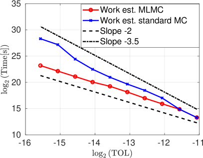
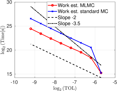
Figure 9: Predicted work of MLMC and MC based on the verification run which resulted in Table 9 for $\mathcal{Q}_{E}$, (Left), and Table 11 for $\mathcal{Q}_{W}$ (Right).

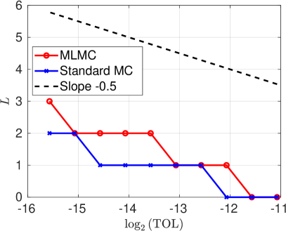
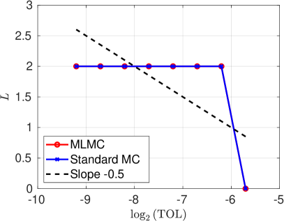
Figure 10: The refinement level, $L$, determining the bias of the estimators, i.e., the maximum refinement level for MLMC and single refinement level for MC, for the sequence of tolerances used for $\mathcal{Q}_{E}$, (Left), and $\mathcal{Q}_{W}$, (Right).

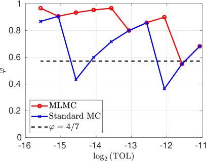
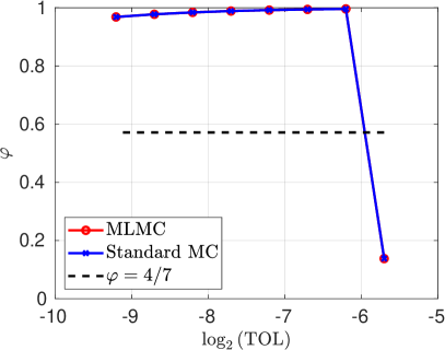
Figure 11: Splitting parameter, $\varphi$, in (30), implicit in the MLMC and MC estimators listed in Table 9 for $\mathcal{Q}_{E}$, (Left), and Table 11 for $\mathcal{Q}_{W}$, (Right). The dashed line denotes the asymptotically optimal value $\varphi=4/7$ for MC, as $\mathrm{TOL}\to 0$, given the asymptotic work and convergence rates.

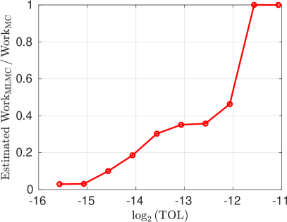
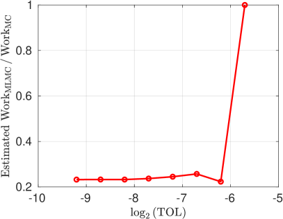
Figure 12: Predicted ratio of MLMC to MC work based on the verification run which resulted in Table 9 for $\mathcal{Q}_{E}$, (Left), and Table 11 for $\mathcal{Q}_{W}$ (Right).

	Samples per level, $N_{\ell}$				$\mathrm{TOL}$	$W_{\mathrm{MLMC}}$
	$\ell=0$	$\ell=1$	$\ell=2$	$\ell=3$		Core Time [s]
$\mathrm{TOL}_{1}$	8	–	–	–	4.650$\cdot 10^{-4}$	8.730$\cdot 10^{3}$
$\mathrm{TOL}_{2}$	24	–	–	–	3.288$\cdot 10^{-4}$	2.995$\cdot 10^{4}$
$\mathrm{TOL}_{3}$	28	3	–	–	2.325$\cdot 10^{-4}$	5.708$\cdot 10^{4}$
$\mathrm{TOL}_{4}$	61	6	–	–	1.644$\cdot 10^{-4}$	1.182$\cdot 10^{5}$
$\mathrm{TOL}_{5}$	141	13	–	–	1.163$\cdot 10^{-4}$	2.688$\cdot 10^{5}$
$\mathrm{TOL}_{6}$	220	20	2	–	8.220$\cdot 10^{-5}$	6.017$\cdot 10^{5}$
$\mathrm{TOL}_{7}$	452	40	2	–	5.813$\cdot 10^{-5}$	1.131$\cdot 10^{6}$
$\mathrm{TOL}_{8}$	941	82	4	–	4.110$\cdot 10^{-5}$	2.230$\cdot 10^{6}$
$\mathrm{TOL}_{9}$	1996	173	7	–	2.906$\cdot 10^{-5}$	4.619$\cdot 10^{6}$
$\mathrm{TOL}_{10}$	3580	311	13	2	2.055$\cdot 10^{-5}$	9.498$\cdot 10^{6}$

Table 9: Parameters defining the MLMC estimator for different tolerances and the resulting work, measured in core time, for the approximation of ${\mathrm{E}\mspace{-2.0mu}\left[\mathcal{Q}_{E}\right]}$. The largest tolerance, $\mathrm{TOL}_{1}$, corresponds to approximately 12.5% of the reference value in Table 13.

	$\ell$	$N_{\ell}$	$\mathrm{TOL}$	$W_{\mathrm{MC}}$, Core Time [s]
$\mathrm{TOL}_{1}$	0	8	4.650$\cdot 10^{-4}$	8.730$\cdot 10^{3}$
$\mathrm{TOL}_{2}$	0	24	3.288$\cdot 10^{-4}$	2.995$\cdot 10^{4}$
$\mathrm{TOL}_{3}$	0	106	2.325$\cdot 10^{-4}$	1.182$\cdot 10^{5}$
$\mathrm{TOL}_{4}$	1	48	1.644$\cdot 10^{-4}$	3.588$\cdot 10^{5}$
$\mathrm{TOL}_{5}$	1	110	1.163$\cdot 10^{-4}$	8.260$\cdot 10^{5}$
$\mathrm{TOL}_{6}$	1	272	8.220$\cdot 10^{-5}$	2.053$\cdot 10^{6}$
$\mathrm{TOL}_{7}$	1	778	5.813$\cdot 10^{-5}$	–
$\mathrm{TOL}_{8}$	1	2978	4.110$\cdot 10^{-5}$	–
$\mathrm{TOL}_{9}$	2	1986	2.906$\cdot 10^{-5}$	–
$\mathrm{TOL}_{10}$	2	4333	2.055$\cdot 10^{-5}$	–

Table 10: Parameters defining the MC estimator for the approximation of ${\mathrm{E}\mspace{-2.0mu}\left[\mathcal{Q}_{E}\right]}$ for different tolerances and the resulting work, measured in core time, in the cases where the MC estimate has been computed.

	Number of samples per level, $N_{\ell}$				$\mathrm{TOL}$	$W_{\mathrm{MLMC}}$
	$\ell=0$	$\ell=1$	$\ell=2$	$\ell=3$		Core Time [s]
$\mathrm{TOL}_{1}$	31	–	–	–	1.920$\cdot 10^{-2}$	3.396$\cdot 10^{4}$
$\mathrm{TOL}_{2}$	–	23	2	–	1.357$\cdot 10^{-2}$	3.373$\cdot 10^{5}$
$\mathrm{TOL}_{3}$	–	46	5	–	9.598$\cdot 10^{-3}$	7.652$\cdot 10^{5}$
$\mathrm{TOL}_{4}$	–	91	9	–	6.787$\cdot 10^{-3}$	1.491$\cdot 10^{6}$
$\mathrm{TOL}_{5}$	–	183	17	–	4.799$\cdot 10^{-3}$	2.790$\cdot 10^{6}$
$\mathrm{TOL}_{6}$	–	368	33	–	3.393$\cdot 10^{-3}$	5.521$\cdot 10^{6}$
$\mathrm{TOL}_{7}$	–	744	67	–	2.399$\cdot 10^{-3}$	1.120$\cdot 10^{7}$
$\mathrm{TOL}_{8}$	–	1519	136	–	1.697$\cdot 10^{-3}$	2.302$\cdot 10^{7}$
$\mathrm{TOL}_{9}$	–	2928	261	2	1.200$\cdot 10^{-3}$	–

Table 11: Parameters defining the MLMC estimator for different tolerances and the resulting work, measured in core time, for the approximation of ${\mathrm{E}\mspace{-2.0mu}\left[\mathcal{Q}_{W}\right]}$. The smallest tolerance, $\mathrm{TOL}_{9}$, is included among the bootstrapped MLMC estimators, but not the primary realizations. The largest tolerance, $\mathrm{TOL}_{1}$, corresponds to approximately 21% of the reference value in Table 13.

	$\ell$	$N_{\ell}$	$\mathrm{TOL}$	$W_{\mathrm{MC}}$, Core Time [s]
$\mathrm{TOL}_{1}$	0	31	1.920$\cdot 10^{-2}$	3.396$\cdot 10^{4}$
$\mathrm{TOL}_{2}$	2	20	1.357$\cdot 10^{-2}$	1.513$\cdot 10^{6}$
$\mathrm{TOL}_{3}$	2	39	9.598$\cdot 10^{-3}$	2.968$\cdot 10^{6}$
$\mathrm{TOL}_{4}$	2	77	6.787$\cdot 10^{-3}$	6.012$\cdot 10^{6}$
$\mathrm{TOL}_{5}$	2	155	4.799$\cdot 10^{-3}$	–
$\mathrm{TOL}_{6}$	2	312	3.393$\cdot 10^{-3}$	–
$\mathrm{TOL}_{7}$	2	632	2.399$\cdot 10^{-3}$	–
$\mathrm{TOL}_{8}$	2	1288	1.697$\cdot 10^{-3}$	–

Table 12: Parameters defining the MC estimator for the approximation of ${\mathrm{E}\mspace{-2.0mu}\left[\mathcal{Q}_{W}\right]}$ for different tolerances and the resulting work, measured in core time, in the cases where the MC estimate has been computed.

5.2.3 MLMC and MC Runs

Here, we present computational results based on the actual MLMC and MC runs performed with the parameters listed in Table 9, for $\mathcal{Q}_{E}$, and Table 11, for $\mathcal{Q}_{W}$.

On the use of parameters estimated in the verification run

Note that we use information from the verification run when we set up the convergence tests. This is in line with the intended use of MLMC in the inverse problem setting that involves repeatedly computing approximate solutions to the underlying forward problem with different parameter values in the course of solving the inverse problem, so that prior information about parameters from earlier runs becomes available. Additionally, a continuation type algorithm [9], can be used in the inverse problem setting.

Computational results

For these tests, one sample of $\mathcal{A}_{MLMC}$ was computed for each tolerance. Note that $\mathcal{A}_{MLMC}$ by itself is a random variable and that here the samples corresponding to different tolerances are independent.

The computational work, shown in Figure 13, agrees very well with the work predicted in Section 5.2.2, due to the highly consistent execution time of SPECFEM2D and the fact that the number of samples on each level was fixed beforehand, based on the verification run results. For those tolerances where both MC and MLMC estimates were computed, significant savings of computational time for MLMC relative to MC was observed, as discussed in Section 5.2.2.

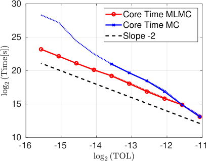
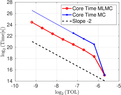
Figure 13: MLMC and MC work as a function of $\mathrm{TOL}$ for the approximation of ${\mathrm{E}\mspace{-2.0mu}\left[\mathcal{Q}_{E}\right]}$ (left) and ${\mathrm{E}\mspace{-2.0mu}\left[\mathcal{Q}_{W}\right]}$ (right). Solid lines show actual computational time, as described in Section 5.2.1, and the dotted line shows the predicted work based on the verification run. The dashed line shows the slope of the optimal complexity for Monte Carlo type methods, $\mathrm{TOL}^{-2}$.

In the absence of an a priori known exact solution to the test problem, we estimate the accuracy of the MLMC results by comparing them to a reference solution obtained by pooling a larger number of samples on each level, including all samples used to generate the MLMC estimators for varying tolerances; see Table 13 on page 13. Thus, while the samples of these estimators are mutually independent, they are not independent of the reference value. On the other hand, the number of samples used to obtain the reference value vastly exceeds the number of samples for larger tolerances and significantly exceeds the number of samples used for the smaller tolerances. The errors compared to this reference solution are shown as red circles in Figure 14.

Additionally, 100 samples of $\mathcal{A}_{MLMC}$ for each value of $\mathrm{TOL}$ were obtained by bootstrapping from the same pool of samples used to generate the reference solution. The corresponding errors, marked with black crosses in Figure 14, indicate the variability of the error.

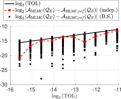
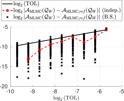
Figure 14: Convergence of the MLMC estimators of Table 9 for ${\mathrm{E}\mspace{-2.0mu}\left[\mathcal{Q}_{E}\right]}$ (left) and Table 11 for ${\mathrm{E}\mspace{-2.0mu}\left[\mathcal{Q}_{W}\right]}$ (right). One realization of $\mathcal{A}_{MLMC}(\mathcal{Q}_{\ast})$ per value of the tolerance was computed, based on samples independent of those used for all other tolerances, and the error was approximated using the reference value of $\mathcal{A}_{MLMC}(\mathcal{Q}_{\ast})$ in Table 13; this error estimate is labeled (indep.). In addition, 100 statistically dependent realizations of $\mathcal{A}_{MLMC}(\mathcal{Q}_{\ast})$ for all tolerances were obtained by bootstrapping with replacement from the whole pool of samples; see Table 14. These bootstrapped error estimates are labeled (B.S.).

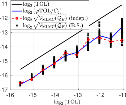
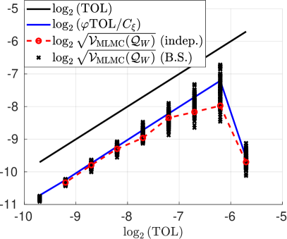
Figure 15: Convergence of the statistical error estimate corresponding to convergence study in Figure 14. Here $\mathcal{V}_{MLMC}$ refers to the estimator of the variance of $\mathcal{A}_{MLMC}(\mathcal{Q}_{\ast})$ in (56), obtained by replacing the true variances by their unbiased estimators (51).

The variance of the MLMC estimator

$${\mathrm{Var}\mspace{-2.0mu}\left[\mathcal{A}_{MLMC}(\mathcal{Q})\right]} =\frac{1}{N_{0}}{\mathrm{Var}\mspace{-2.0mu}\left[\mathcal{Q}_{0}\right]}+\sum_{\ell=1}^{L}\frac{1}{N_{\ell}}{\mathrm{Var}\mspace{-2.0mu}\left[\Delta\mathcal{Q}_{\ell}\right]},$$ (56)

is approximated by sample variances to verify that (46) is satisfied. As shown in Figure 15, $\sqrt{\mathcal{V}_{MLMC}}\approx\frac{\varphi\mathrm{TOL}}{C_{\xi}}$, with $C_{\xi}=2$, consistently with the required constraint on the statistical error, as to be expected based on the sample variance estimates from the verification phase.

For comparison, the corresponding tests for standard MC are shown in Figure 16 and Figure 17. Note in particular, that though the computation here were significantly more expensive than the corresponding MLMC computations, on smaller tolerances, the statistical error was not over-resolved.

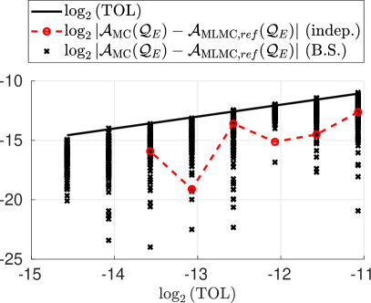
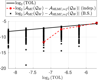
Figure 16: Convergence of the MC estimators of Table 10 for ${\mathrm{E}\mspace{-2.0mu}\left[\mathcal{Q}_{E}\right]}$ (left) and Table 12 for ${\mathrm{E}\mspace{-2.0mu}\left[\mathcal{Q}_{W}\right]}$ (right). One realization of $\mathcal{A}_{MC}(\mathcal{Q}_{\ast})$ per value of the tolerance was computed, based on samples independent of those used for all other tolerances, and the error was approximated using the reference value of $\mathcal{A}_{MLMC}(\mathcal{Q}_{\ast})$ in Table 13; this error estimate is labeled (indep.). In addition, 100 statistically dependent realizations of $\mathcal{A}_{MC}(\mathcal{Q}_{\ast})$ for all tolerances were obtained by bootstrapping with replacement from the whole pool of samples; see Table 14. These bootstrapped error estimates are labeled (B.S.).

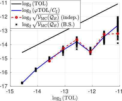
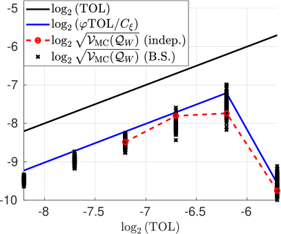
Figure 17: Convergence of the statistical error estimate corresponding to convergence study in Figure 16. Here $\mathcal{V}_{MC}$ refers to the estimator of ${\mathrm{Var}\mspace{-2.0mu}\left[\mathcal{A}_{MC}(\mathcal{Q}_{\ast,L})\right]}=\frac{{\mathrm{Var}\mspace{-2.0mu}\left[(\mathcal{Q}_{\ast,L})\right]}}{N_{L}}$, obtained by unbiased sample variance estimators (51). To control the statistical error, we chose the number of samples so that $\sqrt{\mathcal{V}_{MC}}=\varphi\mathrm{TOL}/C_{\xi}$, for $\mathcal{V}_{MC}$ predicted based on the parameters estimated from the verification run.

	Number of samples per level, $N_{\ell}$				$\mathcal{A}_{MLMC}(\mathcal{Q}_{\ast,ref})$	$\mathcal{V}_{\mathrm{MLMC}}\left(\mathcal{Q}_{\ast,ref}\right)$
	$\ell=0$	$\ell=1$	$\ell=2$	$\ell=3$
$\mathcal{Q}_{E}$	19045	5608	351	4	3.729$\cdot 10^{-3}$	1.31$\cdot 10^{-11}$
$\mathcal{Q}_{W}$	–	5608	351	4	9.227$\cdot 10^{-2}$	1.98$\cdot 10^{-7}$

Table 13: Reference values of ${\mathrm{E}\mspace{-2.0mu}\left[\mathcal{Q}_{E}\right]}$ and ${\mathrm{E}\mspace{-2.0mu}\left[\mathcal{Q}_{W}\right]}$ together with the samples per level in the MLMC estimators used to obtain them.

Number of samples per level, $N_{\ell}$, in pool
	$\ell=0$	$\ell=1$	$\ell=2$	$\ell=3$
MLMC $\mathcal{Q}_{E}$	19045	5608	351	4
MLMC $\mathcal{Q}_{W}$	–	5608	351	4
MC	24653	5959	355	4

Table 14: The number of i.i.d. samples per level in the pool of samples used when bootstrapping the estimators $\mathcal{A}_{MLMC}(\mathcal{Q}_{E})$ and $\mathcal{A}_{MLMC}(\mathcal{Q}_{W})$, where the used number of samples per level are given in Table 9 and Table 11 for $\mathcal{Q}_{E}$ and $\mathcal{Q}_{W}$ respectively.

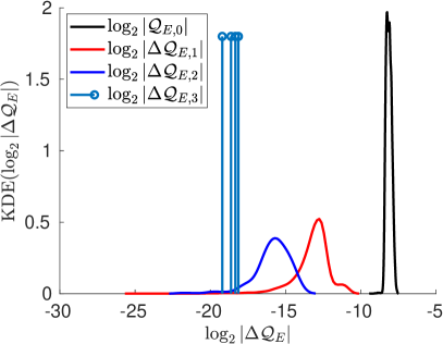
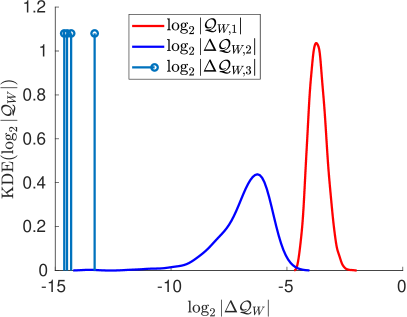
Figure 18: Distribution of the samples of $\Delta\mathcal{Q}_{E}$ and $\Delta\mathcal{Q}_{W}$ used for the bootstrapping of MLMC estimators and for the reference solutions; compare Table 13 and Table 14.

6 Conclusions and Future Work

We have verified experimentally that MLMC techniques can significantly reduce the computational cost of approximating expected values of selected quantities of interest, defined in terms of misfit functions between simulated waveforms and synthetic data with added noise, and where the expected values are taken with respect to random parameters modeling the uncertainties of the Earth’s material properties. The numerical experiments conducted in this work were performed on two-dimensional physical domains, but the extension to three-dimensional physical domains does not create any additional difficulties other than a higher computational cost per sample, due to the numerical approximation of the underlying wave propagation model in higher spatial dimension. Furthermore, the asymptotic complexity of the MLMC method for these particular underlying approximation methods remains the same in the three-dimensional case up to logarithmic factors in the user-specified error tolerance.

Future work includes defining the misfit function between computed waveforms from three-dimensional simulations and actual measurement data obtained in field studies, instead of synthetic data with added noise, thus addressing the associated seismic inversion problem of inferring the source location. Replacing the coarse level samples in the MLMC hierarchies with samples computed using an elastic model will likely further improve the computational gains of MLMC compared to standard MC. Other future work is related to considering alternative ways to define the misfit function between computed and measured seismic signals. In this context, the normalized integration method (NIM), proposed in [30], and other recently proposed optimal transport-based approaches [34] will be considered.

References

- [1] Aki, K., Richards, P.G.: Quantitative Seismology: Theory and Methods, 2 edn. University Science Books (2002)
- [2] Albaric, J., Perrot, J., Déverchère, J., Deschamps, A., Gall, B.L., Ferdinand, R., Petit, C., Tiberi, C., Sue, C., Songo, M.: Contrasted seismogenic and rheological behaviours from shallow and deep earthquake sequences in the North Tanzanian Divergence, East Africa. Journal of African Earth Sciences 58(5), 799 – 811 (2010). DOI 10.1016/j.jafrearsci.2009.09.005. URL http://www.sciencedirect.com/science/article/pii/S1464343X09001824
- [3] Berenger, J.P.: A perfectly matched layer for the absorption of electromagnetic waves. Journal of Computational Physics 114(2), 185 – 200 (1994). DOI 10.1006/jcph.1994.1159. URL http://www.sciencedirect.com/science/article/pii/S0021999184711594
- [4] Bissiri, P.G., Holmes, C.C., Walker, S.G.: A general framework for updating belief distributions. Journal of the Royal Statistical Society: Series B (Statistical Methodology) 78(5), 1103–1130 (2016). DOI 10.1111/rssb.12158. URL https://rss.onlinelibrary.wiley.com/doi/full/10.1111/rssb.12158
- [5] Blanc, E., Komatitsch, D., Chaljub, E., Lombard, B., Xie, Z.: Highly accurate stability-preserving optimization of the zener viscoelastic model, with application to wave propagation in the presence of strong attenuation. Geophysical Journal International 205(1), 427–439 (2016). DOI 10.1093/gji/ggw024. URL https://academic.oup.com/gji/article/205/1/427/2594855
- [6] Brown, T.S., Du, S., Eruslu, H., Sayas, F.-J.: Analysis for models of viscoelastic wave propagation. Applied Mathematics and Nonlinear Sciences 3(1), 55–96 (2018). DOI 10.21042/AMNS.2018.1.00006. URL https://content.sciendo.com/view/journals/amns/3/1/article-p55.xml
- [7] Carcione, J.M.: Wave Fields in Real Media; Wave Propagation in Anisotropic, Anelastic, Porous and Electromagnetic Media, 3 edn. Elsevier Science (2014)
- [8] Carcione, J.M., Kosloff, D., Kosloff, R.: Wave propagation simulation in a linear viscoelastic medium. Geophysical Journal 95(3), 597–611 (1988). DOI 10.1111/j.1365-246X.1988.tb06706.x. URL https://onlinelibrary.wiley.com/doi/abs/10.1111/j.1365-246X.1988.tb06706.x
- [9] Collier, N., Haji-Ali, A.L., Nobile, F., von Schwerin, E., Tempone, R.: A continuation multilevel Monte Carlo algorithm. BIT Numerical Mathematics pp. 1–34 (2014). DOI 10.1007/s10543-014-0511-3. URL https://link.springer.com/article/10.1007/s10543-014-0511-3
- [10] Cruz-Jiménez, H., Li, G., Mai, P.M., Hoteit, I., Knio, O.M.: Bayesian inference of earthquake rupture models using polynomial chaos expansion. Geoscientific Model Development 11(7), 3071–3088 (2018). DOI 10.5194/gmd-11-3071-2018. URL https://www.geosci-model-dev.net/11/3071/2018/
- [11] Dahlen, F.A., Tromp, J.: Theoretical Global Seismology, 2 edn. Princeton University Press (1998)
- [12] Emmerich, H., Korn, M.: Incorporation of attenuation into time-domain computations of seismic wave fields. Geophysics 52(9), 1252–1264 (1987). DOI 10.1190/1.1442386. URL https://library.seg.org/doi/abs/10.1190/1.1442386
- [13] Engquist, B., Froese, B.D., Yang, Y.: Optimal transport for seismic full waveform inversion. Communications in Mathematical Sciences 14(8), 2309–2330 (2016). DOI 10.4310/CMS.2016.v14.n8.a9. URL https://www.intlpress.com/site/pub/pages/journals/items/cms/content/vols/0014/0008/a009/index.php
- [14] Engquist, B., Hamfeldt, B.: Application of the Wasserstein metric to seismic signals. Communications in Mathematical Sciences 12(5), 979–988 (2014). DOI 10.4310/CMS.2014.v12.n5.a7. URL https://www.intlpress.com/site/pub/pages/journals/items/cms/content/vols/0012/0005/a007/
- [15] Fabrizio, M., Morro, A.: Mathematical Problems in Linear Viscoelasticity. Studies in Applied Mathematics. SIAM (1992). DOI 10.1137/1.9781611970807.fm. URL https://epubs.siam.org/doi/10.1137/1.9781611970807.fm
- [16] Giles, M.B.: Multilevel Monte Carlo path simulation. Operations Research 56(3), 607–617 (2008). DOI 10.1287/opre.1070.0496. URL https://pubsonline.informs.org/doi/abs/10.1287/opre.1070.0496
- [17] Giles, M.B.: Multilevel monte carlo methods. Acta Numerica 24, 259–328 (2015). DOI 10.1017/S096249291500001X. URL https://www.cambridge.org/core/journals/acta-numerica/article/multilevel-monte-carlo-methods/C5AF9A57ED8FF8FDF08074C1071C5511
- [18] Haji-Ali, A.L., Nobile, F., von Schwerin, E., Tempone, R.: Optimization of mesh hierarchies in multilevel Monte Carlo samplers. Stochastics and Partial Differential Equations Analysis and Computations 4(1), 76–112 (2016). DOI 10.1007/s40072-015-0049-7. URL https://link.springer.com/article/10.1007/s40072-015-0049-7?email.event.1.SEM.ArticleAuthorContributingOnlineFirst
- [19] Heinrich, S.: Multilevel Monte Carlo Methods, Lecture Notes in Computer Science, vol. 2179, pp. 58–67. Springer (2001). DOI 10.1007/3-540-45346-6˙5. URL https://link.springer.com/chapter/10.1007/3-540-45346-6_5
- [20] Hoel, H., Krumscheid, S.: Central limit theorems for multilevel Monte Carlo methods. Journal of Complexity 54 (2019). DOI 10.1016/j.jco.2019.05.001. URL https://www.sciencedirect.com/science/article/pii/S0885064X19300408
- [21] Hughes, T.J.R.: The Finite Element Method: Linear Static and Dynamic Finite Element Analysis, 2 edn. Dover Civil and Mechanical Engineering. Dover Publications (2000). URL https://books.google.com.sa/books?id=cHH2n_qBK0IC
- [22] Komatitsch, D., Tromp, J.: Introduction to the spectral element method for three-dimensional seismic wave propagation. Geophysical Journal International 139(3), 806–822 (1999). DOI 10.1046/j.1365-246x.1999.00967.x. URL https://onlinelibrary.wiley.com/doi/full/10.1046/j.1365-246x.1999.00967.x
- [23] Komatitsch, D., Tromp, J.: A perfectly matched layer absorbing boundary condition for the second-order seismic wave equation. Geophysical Journal International 154(1), 146–153 (2003). DOI 10.1046/j.1365-246X.2003.01950.x. URL https://onlinelibrary.wiley.com/doi/abs/10.1046/j.1365-246X.2003.01950.x
- [24] Komatitsch, D., Vilotte, J.P.: The spectral element method: An efficient tool to simulate the seismic response of 2D and 3D geological structures. Bulletin of the Seismological Society of America 88(2), 368–392 (1998). DOI 10.1190/1.1820185. URL https://pubs.geoscienceworld.org/ssa/bssa/article/88/2/368/120304/the-spectral-element-method-an-efficient-tool-to
- [25] Komatitsch, D., Vilotte, J.P., Cristini, P., Labarta, J., Le Goff, N., Le Loher, P., Liu, Q., Martin, R., Matzen, R., Morency, C., Peter, D., Tape, C., Tromp, J., Xie, Z.: Specfem2d v7.0.0 (2012).
- [26] Kortas, S.: decimate v0.9.5 [software] (2018). URL https://github.com/KAUST-KSL/decimate
- [27] Lions, J.L., Magenes, E.: Non-homogeneous boundary value problems and applications. Vol. I. Springer-Verlag (1972)
- [28] Lions, J.L., Magenes, E.: Non-homogeneous boundary value problems and applications. Vol. II. Springer-Verlag (1972)
- [29] Liu, H.P., Anderson, D.L., Kanamori, H.: Velocity dispersion due to anelasticity: implications for seismology and mantle composition. Geophysical Journal of the Royal Astronomical Society 47, 41–58 (1976). DOI 10.1111/j.1365-246x.1976.tb01261.x. URL https://academic.oup.com/gji/article/47/1/41/699083
- [30] Liu, J., Chauris, H., Calandra, H.: The Normalized Integration Method - An Alternative to Full Waveform Inversion? In: 25th Symposium on the Application of Geophpysics to Engineering & Environmental Problems, p. Best of 2011 EAGE/NSGD. United States (2012). DOI 10.4133/1.4721678. URL https://library.seg.org/doi/abs/10.4133/1.4721678
- [31] Moczo, P., Robertsson, J.O., Eisner, L.: The finite-difference time-domain method for modeling of seismic wave propagation. In: R.S. Wu, V. Maupin, R. Dmowska (eds.) Advances in Wave Propagation in Heterogenous Earth, Advances in Geophysics, vol. 48, pp. 421–516. Elsevier (2007). DOI 10.1016/S0065-2687(06)48008-0. URL http://www.sciencedirect.com/science/article/pii/S0065268706480080
- [32] Motamed, M., Appelö, D.: Wasserstein metric-driven Bayesian inversion with application to wave propagation problems (2018). ArXiv: 1807.09682 [math.NA]. URL https://arxiv.org/abs/1807.09682
- [33] Motamed, M., Nobile, F., Tempone, R.: A stochastic collocation method for the second order wave equation with a discontinuous random speed. Numerische Mathematik 123(3), 493–536 (2013). DOI 10.1007/s00211-012-0493-5. URL https://link.springer.com/article/10.1007/s00211-012-0493-5
- [34] Métivier, L., Allain, A., Brossier, R., Mérigot, Q., Oudet, E., Virieux, J.: Optimal transport for mitigating cycle skipping in full-waveform inversion: A graph-space transform approach. GEOPHYSICS 83(5), R515–R540 (2018). DOI 10.1190/geo2017-0807.1. URL https://library.seg.org/doi/full/10.1190/geo2017-0807.1
- [35] Roecker, S., Ebinger, C., Tiberi, C., Mulibo, G., Ferdinand-Wambura, R., Mtelela, K., Kianji, G., Muzuka, A., Gautier, S., Albaric, J., Peyrat, S.: Subsurface images of the Eastern Rift, Africa, from the joint inversion of body waves, surface waves and gravity: investigating the role of fluids in early-stage continental rifting. Geophysical Journal International 210(2), 931–950 (2017). DOI 10.1093/gji/ggx220. URL https://academic.oup.com/gji/article/210/2/931/3836409
- [36] Tromp, J., Komatitsch, D., Liu, Q.: Spectral-element and adjoint methods in seismology. Communications in Computational Physics 3(1), 1–32 (2008). URL https://authors.library.caltech.edu/9615/
- [37] Virieux, J.: P-SV wave propagation in heterogeneous media: velocity-stress finite-difference method. Geophysics 51(4), 889–901 (1986). DOI 10.1016/0148-9062(86)92435-6. URL https://www.sciencedirect.com/science/article/pii/0148906286924356?via%3Dihub
- [38] Xie, Z., Komatitsch, D., Martin, R., Matzen, R.: Improved forward wave propagation and adjoint-based sensitivity kernel calculations using a numerically stable finite-element PML. Geophysical Journal International 198(3), 1714–1747 (2014). DOI 10.1093/gji/ggu219 URL https://academic.oup.com/gji/article/198/3/1714/588126
- [39] Xie, Z., Matzen, R., Cristini, P., Komatitsch, D., Martin, R.: A perfectly matched layer for fluid-solid problems: Application to ocean-acoustics simulations with solid ocean bottoms. The Journal of the Acoustical Society of America 140(1), 165–175 (2016). DOI 10.1121/1.4954736. URL https://asa.scitation.org/doi/10.1121/1.4954736
- [40] Yang, Y., Engquist, B.: Analysis of optimal transport and related misfit functions in full-waveform inversion. GEOPHYSICS 83(1), A7–A12 (2018). DOI 10.1190/geo2017-0264.1. URL https://library.seg.org/doi/10.1190/geo2017-0264.1
- [41] Yang, Y., Engquist, B., Sun, J., Hamfeldt, B.F.: Application of optimal transport and the quadratic Wasserstein metric to full-waveform inversion. GEOPHYSICS 83(1), R43–R62 (2018). DOI 10.1190/geo2016-0663.1. URL https://doi.org/10.1190/geo2016-0663.1
- [42] Zhang, C.H., Xie, Z., Komatitsch, D., Cristini, P., Matzen, R.: Revisit the 1/L problem in rheological models for time-domain seismic-wave propagation, pp. 3955–3959. Society of Exploration Geophysicists, 3955-3959 (2016). DOI 10.1190/segam2016-13964889.1. URL https://library.seg.org/doi/abs/10.1190/segam2016-13964889.1