Introduction to Critical Phenomena through the Fiber Bundle Model of Fracture

Abstract

We discuss the failure dynamics of the Fiber Bundle Model, especially in the equal-load-sharing scheme. We also highlight the “Critical” aspects of their dynamics in comparison with those in standard thermodynamic systems undergoing phase transitions.

I Introduction

After receiving the invitation from the Editors to contribute to the special issue on “Complexity” of the European Journal of Physics, we thought that it would be a good idea to introduce the readers, students in particular, to the study of the dynamics of the “Fiber Bundle Model” (FBM) and to their “critical behavior”. We understand that the main focus of this special issue is to present the topic of “Complexity” in a simple way, demonstrating the subtle features of the problems. “Critical Phenomena” nicely demonstrate one important aspect of the complexity of the nature and this is wide enough a field with huge developements in all the fronts: theoretical, numerical and experimental. Thousands of papers, reviews and articles have been published so far on this topic and few hundreds are still being published each year. But introducing critical phenomena to the college, university students or to the beginners is not always easy. Surely, asking them to go through the vast literature does not make sense.

Here comes the role of “models”. We plan to introduce them through a “simple” model which is intuitively appealing and has clear-cut dynamical rules. They allow us to perform some analytic calculations and get solutions. Also it is possible to check the results numerically through a few quick “runs”.

The Fiber Bundle Model (FBM), introduced by Peirce in $1926$ p26 , is such a simple model. Although quite old and even though it was designed as a model for fracture or failure of a set of parallel elements (fibers), each having a breaking threshold different from others, with the collective sharing of the failed fiber’s load, the failure dynamics in the model clearly shows all the attributes of the critical phenaomena and associated phase transition. Indeed, the FBM is the precise equivalent of the Ising model of magnetism, introduced by Ising i25 in 1925. The models are both identically potential, deep and versatile in the respective fields. A recently published book hhp15 tried to gather and explain works on FBM from a “statistical physics” point of view. In this article we want to concentrate only on FBM’s dynamical aspects related to “critical phenomena”. We hope, it will help easy introduction to the models (FBM) and critical phenomena before the students undertake research on these topics. Yes, “students” are the target groups for this article.

We arrange this article as follows: After the short introduction (section I) we briefly introduce the notion of critical phenomena in section II. Then we discuss the brief history of FBM and its evolution as a fracture model in section III. Section IV deals with the simplest version of FBM, the equal-load-sharing FBM. In several sub-sections of section IV we demonstrate the critical behavior in FBM with construction of the evolution dynamics and their solutions. We also compare the analytic results with numerical simulations in this section. We dedicate section V for discussions on some related works which would help to understand the critical behavior of FBM. Finally, some discussions and conclusions will be made in section VI.

II Critical phenomena

Let us consider the case of a ferromagnet. Even in absence of any external field, at temperatures ($T$) below the Courie temperature ($T_{c}$), one gets a finite average magnetisation. This spontaneous magnetisation disappeares as one increases the temperature of the magnet beyond the Curie value. This phase transition (from the ferromagnetic phase with spontaneous magnetisation to paramagnetic phase with vanishing magnetisation) was seen to have some “critical” aspects in the sense that the temperature variation of the magnetisation ($m$) or the susceptibility ($\chi$) near the Curie point can be expressed as power laws with respect to the temperature interval from the Curie (critical) point: $m(T)\sim|T-T_{c}|^{\beta}$, $\chi(T)\sim|T-T_{c}|^{-\gamma}$. Additionally, the values of these powers (exponents) were found to be irrational numbers in general (indicating singular behavior of the free energy of the magnets near the ferro-para transition point). When interpreted in terms of the elemental spin-magnetic moments, which interact through the exchange interactions, one finds that the correlation of the spin-state fluctuations at any arbitrary crystal point and that of another spin at a distance $r$ decayes as $exp[-r/\xi(T)]$, where the correlation length $\xi(T)\sim|T-T_{c}|^{-\nu}$ diverges at $T=T_{c}$ with correlation length exponent $\nu$. This correlation length sets the scale which essentially determines the critical aspects of the thermodynamic behavior near the crirical (Curie) point of the magnet. One also finds values of these exponents ($\beta$, $\gamma$, $\nu$ etc.) are universal in the sense that they depend only on some subtle featurs of the systems like spatial dimensionality of the system and the number of components (dimesionality) of the order parameter (magnetisation) vector. They do not depend on the details like strength of (exchange) interaction, lattice structures, etc.

In the standard models of cooperatively interacting systems in classical statistical physics, like in the Ising model, simple two-state Ising spins (representing the constituent magnetic moments) on the lattice sites interact with themselves through neighboring (exchange) interactions. In absence of any thermal noise, or even at finite but low temperatures, the effect of the (spin-spin) interactions win over thermal noise, and induce spontaneous order without any magnetic field. This order, say ferromagnetic when the spin-spin interactions favor similar orientations of the spins, gets destroyed when the thermal noise, corresponding to a temperature beyond the phase transition or Curie point, wins over and paramagnetic phase sets in. After intensive studies for about three decades, starting middle of the last century, it was established that while the thermodynamic behavior away from the phase transition point of such systems have the usual scale dependent variations (with the finite scale determined by the competitions between the interaction energies and temperature), the behavior become scale free as the phase transition point is approached (see e.g., f17 ) and the behaviors are expressed by power laws (with the powers given by some effective fractal dimensionality m82 of “volume” determined by the “correlation length” scale which diverges at the phase transition point). This scale invariance, often with singularities in the growth of the correlation length scale as one approaches the transition point, had been exploited by the renormalization group theory (see e.g., f17 ; m82 ; wk74 ).

III The Fiber Bundle Model

Figure 1: The Fiber Bundle Model: fibers in parrallel are placed between two solid bars and the load is applied at the lower bar.

The FBM p26 ; phc10 ; hhp15 captures the fracture dynamics in composite materials. In this model, a large number of parallel Hookean springs or fibers are clamped between two horizontal platforms; the upper one (rigid) helps hanging the bundle while the load hangs from the lower one (Figure 1). The springs or fibers are assumed to have identical spring constants though their breaking strengths are different. Once the load per fiber exceeds a fiber’s own threshold, it fails and can not carry load any more. The load it carried is now shared by the surviving fibers. If the lower platform deforms under loading, fibers closer to the just-failed fiber will absorb more of the load compared to those further away and this is called local-load-sharing (LLS) scheme. On the other hand, if the lower platform is rigid, the load is equally distributed to all the surviving fibers. This is called the equal-load-sharing (ELS) scheme. Obviously, for low values of the initial load (per fiber), the successive failures of the fibers due to extra load sharing remain localized and though the strain of the bundle (given by the identical strain of the surviving fibers) grow with increasing load, the bundle as a whole does not fail. Beyond a “critical” value of the initial load, determined by the fiber strength distribution and the load sharing mechanism (after each failures), the successive failures become a global one and the bundle fails. Here, the “order” could be measured by the fraction of eventually surviving fibers (after a “relaxation time” required for stabilization of the bundle), which decreases as the load on the bundle increases. Beyond the critical load, mentioned above, the eventual damage size becomes global and the order disappears (bundle fails). We will see in the following sections, as we approach the critical load (either from higher or lower load), the relaxation time (time or steps required since the load is applied until no further failure occurs or until the whole bundle collapses) diverges with “universal” values of the exponents (power) similar to the power laws in thermodynamic phase transitions discussed in the previous section.

Long back, in $1926$, F. T. Peirce introduced the Fiber Bundle Model p26 to study the strength of cotton yarns in connection with textile engineering. Some static behavior of such a bundle (with equal load sharing by all the surviving fibers, following a failure) was discussed by Daniels in $1945$ d45 and the model was brought to the attention of physicists in $1989$ by Sornette s89 .

IV Equal Load Sharing FBM

Let us consider a fiber bundle model having $N$ parallel fibers placed between two stiff clamps. Each fiber responds linearly with a force $f$ to an extention or stretch $\Delta$,

$$f=\kappa\Delta\;,$$ (1)

where $\kappa$ is the spring constant. We consider $\kappa=1$ for all fibers. Each fiber has a load threshold $x$ assigned to it. If the stretch $\Delta$ exceeds this threshold, the fiber fails irreversibly. In the equal-load-sharing (ELS) mode, the clamps are stiff and there is no non-uniform redistribution of loads among the surviving fibers, i.e., applied load is shared equally by the remaining intact fibers.

IV.1 Fiber strength distributions and the cumulative distributions

The fiber strength thresholds are drawn from a probability density $p(x)$. The corresponding cumulative probability is given by

$$P(y)=\int_{0}^{y}\ p(x)dx\;.$$ (2)

The most studied threshold distributions are Power-law type distributions and Weibull distributions (see Figures 2, 3).

We consider a general power law type fiber threshold distributions within the range $(0,1)$,

$$p(x)\propto x^{\alpha};\alpha\geq 0.$$ (3)

For normalization, we need to fulfil

$$\int_{0}^{1}p(x)dx=1.$$ (4)

Therefore we get, from Eqns. (3, 4), the prefactor is $(1+\alpha)$:

$$p(x)=(1+\alpha)x^{\alpha}.$$ (5)

The cumulative distribution takes the form

$$P(x)=\int_{0}^{x}p(y)dy=x^{1+\alpha}.$$ (6)

When the power-law index $\alpha=0$, the distribution reduces to an uniform distribution with

$$p(x)=1;P(x)=x.$$ (7)

In Figure (2) we present the probability distributions and corresponding cumulative distributions for power-law type threshold distributions.

On the other hand the cumulative Weibull distribution has a form:

$$P(x)=1-\exp(-x^{k}),$$ (8)

where, $k$ is the shape parameter -sometimes called Weibull index. Therefore the probability distribution takes the form:

$$p(x)=kx^{k-1}\exp(-x^{k}).$$ (9)

In figure (3) we present the probability distributions and corresponding cumulative distributions for Weibull threshold distributions.

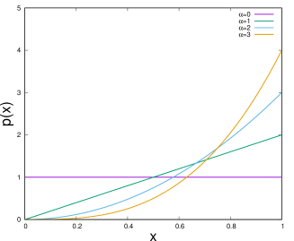
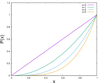
Figure 2: The power-law distributions of fiber thresholds and the corresponding cumulative distributions. The distribution reduces to an uniform distribution when power-law index $\alpha=0$.

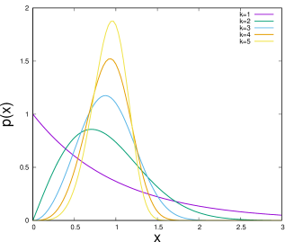
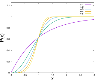
Figure 3: The Weibull distributions of fiber thresholds and the corresponding cumulative distributions.

IV.2 The Load Curve and the Critical values

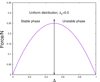
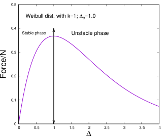
Figure 4: Normalized force vs. extention $\Delta$ for a fiber bundle with uniform and Weibull distributions of thresholds.

When the fiber bundle is loaded, the fibers fail according to their thresholds, the weaker before the stronger. We suppose that $N_{f}$ fibers have failed at a stretch or load $\Delta$. Then the fiber bundle supports a force

$$F=\kappa(N-N_{f})\Delta=(N-N_{f})\Delta,$$ (10)

as the spring constant has been set equal to unity. This is a discrete picture and above equation is valid for any $N$ value, small or large. When $N$ is very large, the force on the bundle at a stretch value $\Delta$ can be written as

$$F=(N-N_{f})\Delta=N(1-P(\Delta))\Delta.$$ (11)

If we plot the normalized force ($F/N$) vs. strech value $\Delta$, we normally get a parabola like shape (Figure 4).

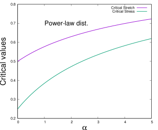
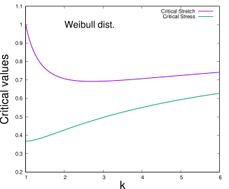
Figure 5: Critical stretch and stress values vs. $\alpha$ (for power-law type distributions) and vs. $k$ for Weibull distributions of thresholds.

The force has a maximum at a particular $\Delta$ value ($\Delta_{c}$) and this is the maximum strength of the whole bundle. This point is often called the failure point or critical point of the system, beyond which the bundle collapses. Therefore we can say -there are two distinct phases of the system: stable phase for $0<\Delta\leq\Delta_{c}$ and unstable phase for $\Delta>\Delta_{c}$. Now, at the critical point, setting $dF(\Delta)/d\Delta=0$ we get

$$1-\Delta_{c}p(\Delta_{c})-P(\Delta_{c})=0.$$ (12)

IV.2.1 General threshold distribution

At the critical stretch $(\Delta_{c})$, we recall Eq. (12) and putting the $p(\Delta_{c})$ and $P(\Delta_{c})$ values for a general power-law type distribution, we get

$$\Delta_{c}=\left(\frac{1}{2+\alpha}\right)^{\frac{1}{1+\alpha}}.$$ (13)

What is the critical strength of the bundle? If we put the $\Delta_{c}$ value in the force expression (Eq. 11), we get

$$\frac{F_{c}}{N}=(1+\alpha)\left(\frac{1}{2+\alpha}\right)^{\frac{2+\alpha}{1+\alpha}}.$$ (14)

Inserting $\alpha=0$, we get

$$\Delta_{c}=\frac{1}{2};\frac{F_{c}}{N}=\frac{1}{4};$$ (15)

which are the critical stretch and force values for uniform distribution (Figures 4, 5).

IV.2.2 Weibull threshold distribution

Let us move to a more general distribution of fiber thresholds, the Weibull distribution, which has been used widely in material science. As the force has a maximum at the failure point $\Delta_{c}$, recalling the expression (Eq. 12) and putting the Weibull $P(x)$, $p(x)$ values into it, we get

$$\exp(-\Delta_{c}^{k})-(\Delta_{c}k\Delta_{c}^{k-1}\exp(-\Delta_{c}^{k}))=0.$$ (16)

From the above equation we can easily calculate the critical stretch value

$$\Delta_{c}=k^{-\frac{1}{k}};$$ (17)

and the critical force value

$$\frac{F_{c}}{N}=k^{-\frac{1}{k}}\exp({-\frac{1}{k}}).$$ (18)

For $k=1$, $\Delta_{c}=1.0$ and $\frac{F_{c}}{N}=\frac{1}{e}$ (Figures 4, 5).

IV.3 Quasi-static loading vs. loading by discrete steps

So far we have described the ELS model and derived the equlibrium Force-elongation or stress-strain relation. We did not say anything about the way of loading, i.e., how the load/force has been applied to the bundle ?

Going back to the history of FBM we find that people discussed first the “weakest-link-failure” mode of loading. This is a very slow loading process that ensures the breaking of only the weakest element (among the intact fibers). This is clearly a “quasi-static” approach and noise or fluctuation in threshold distribution plays a major role (Figure 6) in this type of loading process.

Figure 6: Two realizations for the force per fiber $F(x)/N=\sigma(x)$ as a function of the stretch $x$ for a bundle with $N=50$ having uniform distribution of fiber thresholds. For comparison, a realization with $N=5000$ is shown. Clearly, for large number of fibers, the fluctuations are tiny and the resulting force-stretch curve almost follows the parabolic average force expression $x(1-x)$.

However, a fiber bundle can be loaded in a different way. If a finite external force or load is applied, all fibers that cannot withstand the applied stress, fail. The stress on the surviving fibers then increases, which drives further fibers to break, and so on. This iterative breaking process will go on until an equilibrium with some intact fibers (those can support the load) is reached or the whole bundle collapses. We are now going to study the average behavior of such breaking processes for a bundle of large number of fibers following the formulations in the References pc01 ; bpc03 ; ph07 ; phc10 ; hhp15 .

IV.4 Loading by discrete steps: The recursive dynamics

Let us assume that an external force $F$ is applied to the fiber bundle, with the applied stress denoted by

$$\sigma=F/N,$$ (19)

the external load per fiber. We let $N_{t}$ be the average number of fibers that survive after $t$ steps in the stress redistribution process, with $N_{0}=N$. We want to determine how $N_{t}$ decreases until the degradation process stops.

At a stage during the breaking process when $N_{t}$ intact fibers remain, the effective stress becomes

$$x_{t}=N\sigma/N_{t}.$$ (20)

Thus

$$NP(N\sigma/N_{t})$$ (21)

of fibers will have thresholds that cannot withstand the load. In the next step, therefore, number of intact fibers will be

$$N_{t+1}=N-NP(N\sigma/N_{t}).$$ (22)

Now we define the relative number of intact fibers as

$$n_{t}=N_{t}/N,$$ (23)

therfore, Eqn. (22) takes the form of a nonlinear recursion relation,

$$n_{t+1}=1-P(\sigma/n_{t}),$$ (24)

with $\sigma$ as the control parameter and with $n_{0}=1$ as the start value.

We can also set up a recursion for $x_{t}$, the effective stress $\sigma/n_{t}$ after $t$ iterations:

$$x_{t+1}=\frac{\sigma}{1-P(x_{t})},$$ (25)

with $x_{0}=\sigma$ as the initial value. Since by (20)

$$x_{t}=\sigma/n_{t},$$ (26)

the two recursion relations (24 and 25) may be mapped onto each other.

In general it is not possible to solve nonlinear iterations like (24) or (25) analytically. The model with uniform ($\alpha=0$) and linerly increasing ($\alpha=1$) threshold distributions are however, exceptions.

In nonlinear dynamics the character of an iteration is primarily determined by its fixed points (denoted by *). We are therefore interested in possible fixed points $n^{*}$ of (24), which satisfy

$$n^{*}=1-P(\sigma/n^{*}).$$ (27)

Correspondingly, fixed points $x^{*}$ of the iteration (25) must satisfy

$$x^{*}=\frac{\sigma}{1-P(x^{*})},$$ (28)

which may be written as

$$F=N\sigma=Nx^{*}(1-P(x^{*})).$$ (29)

This is precisely the relation (11) between stress and strain. Therefore the equilibrium value of $x$, for a given external stress $\sigma$, is a fixed point.

IV.5 Solution of the recursive dynamics and the Critical exponents

Let us illustrate these general results by an example. We consider first a power-law type distribution (5)

$$p(x)=(1+\alpha)x^{\alpha};P(x)=x^{\alpha+1}.$$ (30)

The fixed-point equation (27) takes the form

$$(n^{*})^{\alpha+2}-(n^{*})^{\alpha+1}+\sigma^{\alpha+1}=0.$$ (31)

If we set $\alpha=0$, the threshold distribution reduces to an uniform threshold distribution and the recursion relation becomes

$$n_{t+1}=1-\sigma/n_{t}.$$ (32)

Consequently the fixed point equation assumes a harmless form

$$(n^{*})^{2}-n^{*}+\sigma=0,$$ (33)

with solution

$$n^{*}={\textstyle\frac{1}{2}}\pm\left(\sigma_{c}-\sigma\right)^{1/2}.$$ (34)

Here $\sigma_{c}=1/4$, the critical value of the applied stress beyond which the bundle fails completely. In (34) the upper signs give $n^{*}>n_{c}$ which corresponds to stable fixed points. The -ve sign in (34) is unphysical as for $\sigma=0$ it gives $n^{*}=0$. From this solution we can easily derive order parameter, susceptibility and relaxation time behavior and their exponents.

IV.5.1 Order parameter

From the fixed-point solution we get at the critical point ($\sigma=\sigma_{c}$)

$$n_{c}^{*}=\frac{1}{2}.$$ (35)

Therefore we can present the fixed-point solution as

$$n^{*}(\sigma)-n_{c}^{*}\propto(\sigma_{c}-\sigma)^{\beta},\hskip 22.76219pt\beta={\textstyle\frac{1}{2}},$$ (36)

where $n^{*}(\sigma)-n_{c}^{*}$ behaves like an order parameter, i.e., it shows a transition from non-zero to zero value at the critical point $\sigma_{c}$.

IV.5.2 Susceptibility

We can define the breakdown susceptibility as $\chi=-dn^{*}/d\sigma$. From the fixed-point solution we can write directly

$$\chi\propto(\sigma_{c}-\sigma)^{-\gamma},\hskip 22.76219pt\gamma={\textstyle\frac{1}{2}};$$ (37)

which diverges at the critical point following a well-defined power law. This is another robust signature of a critical phenomenon.

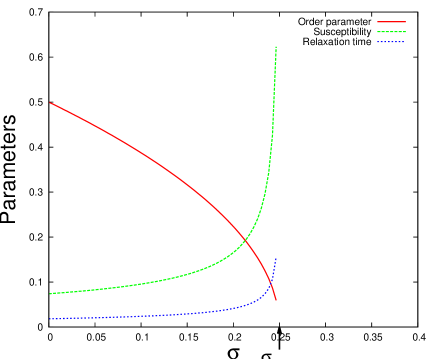
Figure 7: Variation of order parameter, susceptibility and relaxation time vs. applied stress $\sigma$ for uniform distribution of fiber strengths.

IV.5.3 Relaxation time

To track down the approach very near a fixed point, we note that close to a stable fixed point the iterated quantity changes by tiny amounts, so that one may expand in the differences $n_{t}-n^{*}$. For the model with uniform distribution of the thresholds, the recursion relation (24),

$$n_{t+1}=1-\sigma/n_{t},$$ (38)

gives to linear order

$$n_{t+1}-n^{*}=\frac{\sigma}{n^{*}}-\frac{\sigma}{n_{t}}=\frac{\sigma}{n_{t}n^{*}}\;(n_{t}-n^{*})\simeq\frac{\sigma}{n^{*2}}(n_{t}-n^{*}).$$ (39)

Thus the fixed point is approached monotonously with exponentially decreasing steps:

$$n_{t}-n^{*}\propto e^{-t/\tau},$$ (40)

with a relaxation parameter

$$\tau=1/\ln(n^{*2}/\sigma)=1\Big{/}\ln\left[\left({\textstyle\frac{1}{2}}+\sqrt{{\textstyle\frac{1}{4}}-\sigma}\right)^{2}\Big{/}\sigma\right].$$ (41)

For the critical load, $\sigma=\sigma_{c}=\frac{1}{4}$, the argument of the logarithm is $1$, so that apparently $\tau$ is infinite. More precisely, for $\sigma\rightarrow\sigma_{c}$

$$\tau\simeq{\textstyle\frac{1}{4}}\;(\sigma_{c}-\sigma)^{-\theta}\hskip 14.22636pt\mbox{ with }\hskip 8.53581pt\theta={\textstyle\frac{1}{2}}.$$ (42)

The divergence is a clear indication that the character of the breaking dynamics changes when the bundle goes critical.

IV.5.4 Critical slowing

How does the system behave at the critical point ? If we put the critical $\sigma$ value in the recursive equation, we get

$$n_{t}-n_{c}^{*}\sim t^{-\phi},\phi=1,$$ (43)

which implies the relaxation dynamics is critically slow exactly at the critical stress value. Critical-slowing is another known characteristic of a critical phenomenon.

IV.6 Universality

So far we obtained the dynamic critical behavior for the uniform distribution of the breaking thresholds, and the natural question is how general the results are. We can do a spot check on universality through considering a different distribution of fiber strengths. By setting $\alpha=1$, the power-law type distribution reduces to a linearly increasing distribution on the interval $(0,1)$,

$$p(x)=\left\{\begin{array}[]{ll}2x,&\hskip 14.22636pt0\leq x\leq 1\\ 0&\hskip 14.22636ptx>1.\end{array}\right.$$ (44)

For simplicity nondimensional variables are used. By the force-elongation relationship the average total force per fiber,

$$F(x)/N=\left\{\begin{array}[]{ll}x(1-x^{2})&\hskip 14.22636pt0\leq x\leq 1\\ 0&\hskip 14.22636ptx>1,\end{array}\right.,$$ (45)

shows that the critical point is

$$x_{c}=\frac{1}{\sqrt{3}},\hskip 22.76219pt\sigma_{c}=\frac{2}{3\sqrt{3}}.$$ (46)

In this case the recursion relation takes the form

$$n_{t+1}=1-(\sigma/n_{t})^{2},$$ (47)

consequently the fixed-point equation reduces to

$$(n^{*})^{3}-(n^{*})^{2}+\sigma^{2}=0.$$ (48)

a cubic equation in $n^{*}$. Therefore there exist three solutions of $n^{*}$ for each value of $\sigma$. For the critical load, $\sigma_{c}=2/3\sqrt{3}$, the only real and positive solution of (48) is

$$n^{*}_{c}={\textstyle\frac{2}{3}}.$$ (49)

One can show that for $\sigma<\sigma_{c}$ there will be an unstable fixed point with $n^{*}<n^{*}_{c}$, and a stable one with $n^{*}>n^{*}_{c}$.

To find the number of intact fibers in the neighborhood of the critical point, we insert $n=\frac{2}{3}+(n-n_{c})$ into (47), with the result

$${\textstyle\frac{4}{27}}-(n-n_{c})^{2}-(n-n_{c})^{3}=\sigma^{2}=({\textstyle\frac{2}{3\sqrt{3}}}+\sigma-\sigma_{c})^{2}={\textstyle\frac{4}{27}}+{\textstyle\frac{4}{3\sqrt{3}}}(\sigma-\sigma_{c})+(\sigma-\sigma_{c})^{2}.$$ (50)

To leading order we have

$$(n-n_{c})^{2}={\textstyle\frac{4}{3\sqrt{3}}}(\sigma_{c}-\sigma).$$ (51)

IV.6.1 Order parameter

Hence for $\sigma\leq\sigma_{c}$ the order parameter behaves as

$$n(\sigma)-n_{c}\propto(\sigma_{c}-\sigma)^{\beta},\hskip 22.76219pt\beta={\textstyle\frac{1}{2}},$$ (52)

in accordance with (36).

IV.6.2 Susceptibility

The breakdown susceptibility $\chi=-dn/d\sigma$ will therefore have the same critical behavior,

$$\chi\propto(\sigma_{c}-\sigma)^{-\gamma},\hskip 22.76219pt\gamma={\textstyle\frac{1}{2}}$$ (53)

as for the model with a uniform distribution of fiber strengths.

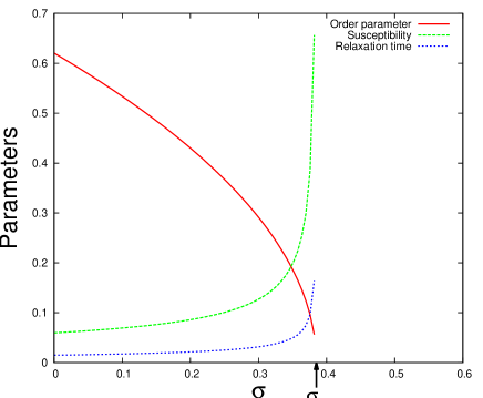
Figure 8: Variation of order parameter, susceptibility and relaxation time vs. applied stress $\sigma$ for linearly increasing fiber strength distribution.

IV.6.3 Relaxation time

Let us also investigate how the stable fixed point is approached. From (47) we find

$$n_{t+1}-n^{*}=\frac{\sigma^{2}}{n^{*2}}-\frac{\sigma^{2}}{n_{t}^{2}}=\frac{\sigma^{2}}{n^{*2}n_{t}^{2}}\;(n_{t}^{2}-n^{*2})\simeq(n_{t}-n^{*})\;\frac{2\sigma^{2}}{n^{*3}}$$ (54)

near the fixed point. Hence the approach is exponential,

$$n_{t}-n^{*}\propto e^{-t/\tau}\hskip 22.76219pt\mbox{with }\hskip 11.38109pt\tau=\frac{1}{\ln(n^{*3}/2\sigma^{2})}.$$ (55)

At the critical point, where $n_{c}^{*}=2/3$ and $\sigma_{c}=2/3\sqrt{3}$, the argument of the logarithm equals $1$, so that $\tau$ diverges when the critical state is approached. The divergence is easily seen to be of the same form,

$$\tau\propto(\sigma_{c}-\sigma)^{-\theta},\theta={\textstyle\frac{1}{2}},$$ (56)

as for the model with a uniform threshold distribution, equation (42).

IV.6.4 Critical slowing

To find the correct behavior of the distance to the critical point, $\Delta n_{t}=n_{t}-n_{c}=n_{t}-2/3$, at criticality, we use the iteration (47) with $\sigma=\sigma_{c}$,

$$n_{t+1}=1-\frac{4/27}{n_{t}^{2}},\hskip 22.76219pt\mbox{ or }\hskip 11.38109pt\Delta n_{t+1}=\frac{1}{3}-\frac{4/27}{(\frac{2}{3}+\Delta n_{t})^{2}}.$$ (57)

Near the fixed point, the deviation $\Delta n_{t}=n_{t}-n^{*}$ is small. An expansion to second order in $\Delta n_{t}$ yields

$$\Delta n_{t+1}=\Delta n_{t}-{\textstyle\frac{9}{4}}\Delta n_{t}^{2},$$ (58)

which is satisfied by

$$\Delta n_{t}=\frac{4}{9t}+{\cal O}(t^{-2}).$$ (59)

The slow critical relaxation towards the fixed point,

$$n_{t}-n_{c}\propto t^{-\phi},\phi=1,$$ (60)

for large $t$, is the same as for the uniform threshold distribution, formula (43).

In conclusion, we have found that the model with a linearly increasing distribution of the fiber strengths possesses the same critical power laws as the model with a uniform distribution. This suggests that the critical properties are universal.

IV.7 Graphical solutions of the recursive dynamics

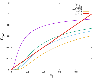
Figure 9: Graphical solution of the ELS recursive dynamics for Weibull distribution.

Even if the recursive dynamics can not be solved for each and every fiber thresold distributions, through a graphical solution scheme one can always reach the critical points. The trick is to plot $n_{t+1}$ vs. $n_{t}$ and check where this plot touches the fixed-point line $n_{t+1}=n_{t}$. For example, let us consider a Weibull distribution (with $k=1$) of fiber thresholds (8), having cumulative distribution

$$P(x)=1-\exp(-x).$$ (61)

When an external stress $\sigma$ is applied, the recursion relation can be written as:

$$n_{t+1}=1-[1-\exp(-\sigma/n_{t}]=\exp(-\sigma/n_{t}).$$ (62)

Now we plot $n_{t+1}$ vs. $n_{t}$ following Eqn. 62 for several $\sigma$ values (see Figure 9). It is clear that at a particular $\sigma$ value, the $n_{t+1}$ vs. $n_{t}$ curve touches the $n_{t+1}=n_{t}$ straight line at a single point and this particular $\sigma$ value is the critical stress value $\sigma_{c}$ for this model.

IV.8 Approach to the critical point

It is important to find out how the system is approaching the critical point (failure point) from below (pre-critical) and above (post-critical) stress values.

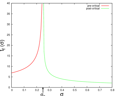
Figure 10: Approach to critical point from below (pre-critical state) and from above (post-critical state) confirms two-sided critical divergence of the recursive step values.

For uniform fiber strength distribution when the external load approaches the critical load $\sigma_{c}=1/4$ from a higher value, i.e., in the post-critical region, the number of necessary iterations increases as one approaches critical point. Near criticality, number of iterations has a square-root divergence ph07 :

$$t_{f}\simeq{\textstyle\frac{1}{2}}\pi(\sigma-\sigma_{c})^{-1/2}.$$ (63)

Similarly, in the pre-critical region, when the external load approaches the critical load $\sigma_{c}=1/4$ from a lower value, near the critical point the number of iterations has again a square root divergence ph07 (for uniform distribution),

$$t_{f}={\textstyle\frac{1}{4}}\;\ln(N)\,(\sigma_{c}-\sigma)^{-1/2},$$ (64)

with a system-size-dependent amplitude.

We therefore find that in FBM, there exists a two-sided critical divergence behavior (Figure 10) in terms of the number of iteration steps needed to reach critical point from below (pre-critical) and above (post-critical) the critical point. Detailed derivation of the above divergences in $t_{f}$ are given in the Appendix.

IV.9 Percolation in Equal Load Sharing FBM

We will now discuss the connection between the Equal Load Sharing Fiber Bundle Model and the standard percolation model.

In the ELS mode, when the fiber bundle is loaded, the fibers fail according to their thresholds, the weaker before the stronger. At a load or stretch $\Delta$, the fiber bundle supports a force

$$F=N\left[1-P(\Delta)\right]\Delta,$$ (65)

where spring constant ($\kappa$) has been set to unity. Clearly, $P(\Delta)$ is the fraction of failed fibers at a load (extension) $\Delta$. We know that there is a certain $\Delta=\Delta_{c}$ value beyond which catastrophic failure occurs and the system collapses completely. We are particularly interested to know whether the cluster of broken fibers percolates in the stable phase (before the failure point is reached) or not? To answer this question we need to calculate $P(\Delta_{c})$. From our analysis in section IV.B, we recall that the force has a parabolic maximum at the failure point $\Delta_{c}$, where the following relation is valid:

$$1-\Delta_{c}p(\Delta_{c})-P(\Delta_{c})=0.$$ (66)

Therefore

$$P(\Delta_{c})=1-\Delta_{c}p(\Delta_{c}).$$ (67)

IV.9.1 General threshold distribution

We consider a general power law type fiber threshold distributions within the range $(0,1)$,

$$p(x)=(1+\alpha)x^{\alpha};P(x)=x^{1+\alpha}.$$ (68)

Putting the $p(\Delta_{c})$ and $P(\Delta_{c})$ values in eq. (66 ) we get

$$\Delta_{c}=\left(\frac{1}{2+\alpha}\right)^{\frac{1}{1+\alpha}}.$$ (69)

From the above relations, we can easily calculate the fraction of failed fibers at the failure point

$$P(\Delta_{c})=\frac{1}{2+\alpha}\leq\frac{1}{2}.$$ (70)

It is obvious that if $P(\Delta_{c})<p_{c}$, ($p_{c}$ is the percolation threshold) largest cluster of broken fibers does not percolate until the failure point itself is reached. Therefore in case of power-law type distribution of thresholds, we do not see percolation of broken fibers in 2D until the system enters into unstable phase. In three dimensional bond-percolation problem the situation is different -as long as $\alpha<1.25$ cluster of brken fibers percolates in the stable phase (Figure (11)).

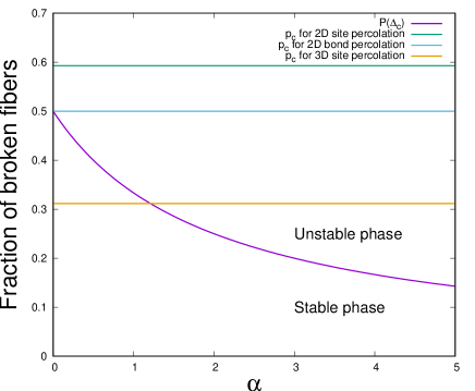
Figure 11: Fraction of broken fibers vs. power law index $\alpha$. The curved line is $P(\Delta_{c})$, which seperates the stable and unstable phases of the FBM. Straight lines are the percolation threshold values.

IV.9.2 Analaysis for Weibull threshold distribution

Let us move to a more general distribution of fiber thresholds, the Weibull distribution. The cumulative Weibull distribution has a form:

$$P(x)=1-\exp(-x^{k}),$$ (71)

where, $k$ is the shape parameter. Therefore the probability distribution takes the form:

$$p(x)=kx^{k-1}\exp(-x^{k}).$$ (72)

As the force has a maximum at the failure point $\Delta_{c}$, recalling the expression (Eq. 12) and putting the $P(x)$, $p(x)$ values into it, we get

$$\exp(-\Delta_{c}^{k})-(\Delta_{c}k\Delta_{c}^{k-1}\exp(-\Delta_{c}^{k})=0.$$ (73)

From the above equation we can easily calculate the critical extention value as

$$\Delta_{c}=k^{-1/k}.$$ (74)

The fraction of fibers at the failure point is

$$P(\Delta_{c})=1-\exp(-\frac{1}{k}).$$ (75)

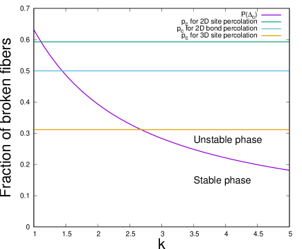
Figure 12: Fraction of broken fibers vs. Weibull index $k$. The curved line is $P(\Delta_{c})$, which seperates the stable and unstable phases of the FBM. Straight lines are the percolation threshold values.

In case of Weibull distribution of fiber thresholds, the clusters of broken fibers can percolate before the failure point is reached (for two and three dimensional site and bond percolation scenarios) when $k$ value remains within a certain window (Figure (12)).

V Some related works on FBM

In this section we would like to bring attention to some related works on FBM which, we believe, may be regarded as essential reading in this field. If we follow quasi-static loading, the ELS model produces avalanches (successive failure of fibers at a fixed external load) of different sizes during the entire fiber-failure process. The statistics of such avalanches were analysed by Hemmer and Hansen in their seminal paper in $1992$ hh92 . They found that the avalanches follow universal power law with exponent $-5/2$ for a mild restriction on the threshold distribution such that the load-curve (force vs. elongation) has single maximum. Later, Pradhan, Hansen and Hemmer showed that the exponent of avalnche distribution crosses over from $-5/2$ to $-3/2$ if we collect only the avalanches near the critical (failure) point phh05 . Also, Divakaran and Dutta studied dd07 the effect of discontinuity in the threshold distribution and obtained similar crossover behavior of avalanche distributions in ELS models.

In $1991$, Harlow and Phoenix first introduced the Local-Load-Sharing (LLS) model hp91 with a simple breaking rule: when a fiber fails, the load it carried is shared by the nearest surviving fibers. The localized load-redistribution mechanism in LLS scheme makes the model very different from the ELS one. In one dimension, the critical strength of the LLS bundle shows a typical system size dependence gip93 ; phc10 : $\sigma_{c}(N)\sim 1/\ln(N)$, where $N$ is the total number of fibers in the chain. However, recent studies by NTNU group have established that in higher dimensions, memory independent LLS model shows non-zero critical strength skh15 . Biswas and Chakrabarti have studied the self-organized dynamics bc13 in LLS models by modifying the load-redistribution rule a bit, where the steadily increasing external load is applied at a central point of the system. The redistributed load always remains localized along the steadily growing boundary of the broken patch and dynamic self-organization sets in.

There have been some attempt to bridge the gap between ELS and LLS models by introducing some intermediate load-sharing rules. Hidalgo, Kun and Herrmann proposed a model hkh02 where the load that was carried by a broken fiber is redistributed to the surviving fibers following a decaying power law in the distance from the broken fiber. In the same line, Pradhan, Chakrabarti and Hansen introduced a mixed-mode model pch05 where the ELS and LLS schemes are mixed together: When a fiber fails a fraction $g$ of the load it carried is distributed according to the LLS rule (to the fibers at the edge of the hole containg the broken fiber) and the rest $1-g$ fraction of the load is distributed to all the surviving fibers. Clearly, for $g=0$, the model reduces to a pure ELS model and for $g=1$, it is nothing but the LLS model. They found an interesting result that the mixed mode model crosses over from ELS to LLS behavior at $g\simeq 0.8$.

Roy and Ray tried to see another type of critical behavior rr15 in ELS model in terms of brittle to quasi-brittle transition as a function of the width of the threshold distribution. Their claim is that at (and below) a critical width value ($\delta_{c}$), breaking of the weakest fiber leads to complete failure of the bundle and at $\delta_{c}$, relaxation time diverges obeying finite- size scaling law: $\tau\sim N^{\beta}(|\delta-\delta_{c}|N^{\alpha})$ with $\alpha=\beta=1/3$.

In section IV we have presented a mean-field treatment of the relaxation behavior of ELS models when the model is loaded by a discrete step. However, one can expect finite-size dependence of the relaxation behavior at or around the critical stress values when the system size is not large enough. Roy, Kundu and Manna have done extensive numerical studies rkm13 on the finite-size scaling forms of the relaxation time as a function of the deviation of stress values from the critical stress for the ELS model. In Ref bs15 Biswas and Sen investigated, mostly analytically, the maximum strength and corresponding redistribution schemes for sudden and quasistatic loading on FBM. The universality class associated with the phase transition from partial to total failure (by increasing the load) was found to be dependent on the redistribution mechanism.

The FBM has also been applied to traffic-jam modelling c06 , power-grid failure modelling pss14 , earthquake modelling, s92 etc. For a recent discussion on self-organized criticalities in FBM, for studying the propagation of crack front in heterogeneous solids, see pp18 . An elegant Renormalization Group Procedure in equal-load-sharing FBM analysis has been introduced in a very recent article phr18 .

VI Discussions

The FBM is an extremely elegant model for studying the collective dynamical failure in inhomogeneus materials. The ELS scheme (ensured by the absolute rigidity of the platforms) of equally sharing of the extra load by the surviving fibers, after an individual fiber failure, allows often some precise analysis of the dynamics. With simple (uniform) fiber breaking threshold distribution, we have demonstrated here the “critical behavior” and its related features like universality. The model here fits simple common sense, yet the collective failure dynamics in the bundle, its critical behavior, are extremely intriguing. Hope, the uninitiated readers can appreciate the excitement.

The same model with realistic fiber threshold distribution (like Weibull distribution or Gumble distribution) may not always allow such analytic studies, but their numerical analysis (often with realistic LLS scheme for load sharing due to local deformations of the platforms with finite rigidity) can take one to the frontiers of civil engineering applications, as had been practiced by the professional engineers and architects.

It may be noted, there is hardly any other model in science and technology, where some simplifications allow intriguing progress analytically in basic science, yet with some realistic ingredients added to the same model, it takes one to the forefront of engineering applications.

VII Acknowledgments

The authors thank Alex Hansen for interesting discussions. This work was partly supported by the Research Council of Norway through its Centers of Excellence funding scheme, project number 262644. BKC is grateful to J. C. Bose Fellowship Grant for support.

VIII Appendix

Appendix A Exact solutions for pre and post-critical relaxation

The iterative breaking process considered in section IV ends with one of two possible end results. Either the whole bundle breaks down, or an equilibrium situation with a finite number of intact fibers is reached. The final fate depends on whether the external stress $\sigma$ on the bundle is postcritical ($\sigma>\sigma_{c}$), precritical ($\sigma<\sigma_{c}$), or critical $\sigma=\sigma_{c}$. We now investigate the total number $t_{f}$ of iterative steps $t$ necessary to reach the final state, and start with the postcritical situation following the formulations in References ph07 ; hhp15 .

A.1 Postcritical relaxation

For uniform threshold distribution (7) we can explicitly and exactly follow the path of iteration. We introduce a measure $\epsilon$ of the deviation from critical value by

$$\epsilon=\sigma-\sigma_{c}=\sigma-{\textstyle\frac{1}{4}},$$ (76)

where $\epsilon$ is positive. The basic iteration formula (24) is in this case

$$n_{t+1}=1-\sigma/n_{t}.$$ (77)

The fraction $n_{t}$ of intact fibers will decrease under the iteration, and we see from (77) that if $n_{t}$ reaches the value $\sigma$ or a smaller value, the next iteration yields $n_{t+1}=0$ or a negative value, i.e. complete bundle breakdown. We wish to find how many iterations, $t_{f}$, is needed to reach this stage.

For that purpose we solve the nonlinear iteration (77) by converting it into a linear iteration by means of two transformations. From (77), we can write

$$n_{t+1}n_{t}=n_{t}-\sigma=n_{t}-{\textstyle\frac{1}{4}}-\epsilon.$$ (78)

We introduce first

$$n_{t}={\textstyle\frac{1}{2}}-y_{t}\sqrt{\epsilon},$$ (79)

with the result

$$2\sqrt{\epsilon}=\frac{y_{t+1}-y_{t}}{1+y_{t+1}y_{t}}.$$ (80)

As a second transformation we put

$$y_{t}=\tan v_{t},$$ (81)

with the result

$$2\sqrt{\epsilon}=\frac{\tan v_{t+1}-\tan v_{t}}{1+\tan v_{t+1}\;\tan v_{t}}=\tan(v_{t+1}-v_{t}).$$ (82)

Hence we have now obtained the linear iteration

$$v_{t+1}-v_{t}=\tan^{-1}(2\sqrt{\epsilon}),$$ (83)

with solution

$$v_{t}=v_{0}+t\tan^{-1}(2\sqrt{\epsilon}).$$ (84)

The iteration starts with all fibers intact, i.e. $n_{0}=1$, which by (79) and (81) corresponds to $y_{0}=-1/2\sqrt{\epsilon}$ and $v_{0}=-\tan^{-1}(1/2\sqrt{\epsilon})$. With the constant in (84) now determined, we can express the solution in terms of the original variable:

$$n_{t}={\textstyle\frac{1}{2}}-\sqrt{\epsilon}\tan\left[-\tan^{-1}(1/2\sqrt{\epsilon})+t\;\tan^{-1}(2\sqrt{\epsilon})\right].$$ (85)

We saw above that when $n_{t}$ obtains a value in the interval $(0,\sigma)$, the next iteration gives $n_{t+1}\leq 0$, complete bundle failure. $n_{t}$ reaching the smallest value $0$ gives an upper bound $t_{f}^{u}$ for the number of iterations. We find

$$t_{f}^{u}(\sigma)=1+\frac{2\tan^{-1}(1/2\sqrt{\epsilon})}{\tan^{-1}(2\sqrt{\epsilon)}}.$$ (86)

And $n_{t}$ reaching the value $\sigma\equiv{\textstyle\frac{1}{2}}+\epsilon$ gives a lower bound:

$$t_{f}^{l}(\sigma)=1+\frac{\tan^{-1}\left[({\textstyle\frac{1}{4}}-\epsilon)/\sqrt{\epsilon}\right]+\tan^{-1}(1/2\sqrt{\epsilon})}{\tan^{-1}(2\sqrt{\epsilon})}.$$ (87)

Figure 13: Post-critical relaxation: Numerical data are for a bundle with $N=10^{6}$ fibers having uniform threshold distribution and averages are taken over $10^{5}$ samples.

The upper and lower bounds (86) and (87) nicely embrace the simulation results (Figure (13)). When the external load is large, just a few iterations suffice to induce completely bundle breakdown. On the other hand, when the external load approaches the critical load $\sigma_{c}=1/4$, the number of necessary iterations becomes vary large. Near criticality ($\epsilon\rightarrow 0$) both the upper and lower bounds, (86) and (87), have a square-root divergence:

$$t_{f}\simeq{\textstyle\frac{1}{2}}\pi(\sigma-\sigma_{c})^{-1/2},$$ (88)

to dominating order for small $\epsilon$.

A.2 Precritical relaxation

When the external stress is less than the critical one, $\sigma<\sigma_{c}$ we use the positive parameter

$$\epsilon=\sigma_{c}-\sigma$$ (89)

as a measure of the deviation from criticality. In this case the bundle is expected to relax to an equilibrium situation with a finite number of fibers intact. We are going to calculate how many iteration $t_{f}$ are needed to reach equilibrium.

Here we consider the uniform threshold distribution (7), and again we transform the nonlinear iteration (38) to a linear one by means of two transformations. Introducing $\sigma={\textstyle\frac{1}{4}}-\epsilon$ and

$$n_{t}={\textstyle\frac{1}{2}}+\sqrt{\epsilon}\;/z_{t}$$ (90)

into (38), we have

$$2\sqrt{\epsilon}=\frac{z_{t+1}-z_{t}}{1-z_{t+1}z_{t}}.$$ (91)

A second transformation,

$$z_{t}=\tanh w_{t},$$ (92)

gives

$$2\sqrt{\epsilon}=\frac{\tanh w_{t+1}-\tanh w_{t}}{1-\tanh w_{t+1}\tanh w_{t}}\equiv\tanh(w_{t+1}-w_{t}).$$ (93)

Hence we have the linear iteration $w_{t+1}-w_{t}=\tanh^{-1}(2\sqrt{\epsilon})$, which gives

$$w_{t}=w_{0}+t\;\tanh^{-1}(2\sqrt{\epsilon}).$$ (94)

As $\tanh^{-1}x=\frac{1}{2}\,\ln[(1+x)/(1-x)]$, via (90) and (92) the initial situation with no broken fibers, $n_{0}=1$, corresponds to $w_{0}=\tanh^{-1}(2\sqrt{\epsilon})$, so that (94) becomes

$$w_{t}=(1+t)\;\tanh^{-1}(2\sqrt{\epsilon}).$$ (95)

For the original variable this corresponds to

$$n_{t}=\frac{1}{2}+\frac{\sqrt{\epsilon}}{\tanh[(1+t)\tanh^{-1}(2\sqrt{\epsilon})]}.$$ (96)

After an infinite number of iterations ($t\rightarrow\infty$ in (96)) $n_{t}$ apparently approaches the fixed point

$$n^{*}={\textstyle\frac{1}{2}}+\sqrt{\epsilon},$$ (97)

which is the fixed point (34) for the uniform distribution. However, the bundle contains merely a finite number of fibers, so equilibrium should be reached after a finite number of steps. Since an equilibrium value corresponds to a fixed point, we seek fixed points $N^{*}$ for finite $N$.

Taking into account that the variables $N_{t}$ are integers, one can get the final result (see ph07 ; hhp15 )

$$t_{f}(\sigma)=-1+\frac{\ln(N)}{2\tanh^{-1}(2\sqrt{\epsilon})}.$$ (98)

The simulation data in Figure (14) for the uniform threshold distribution are well approximated by this analytic formula. Equation (98) shows that near the critical point the number of iterations has again a square root divergence,

$$t_{f}={\textstyle\frac{1}{4}}\;\ln(N)\,(\sigma_{c}-\sigma)^{-1/2},$$ (99)

with a system-size-dependent amplitude.

Figure 14: Pre-critical relaxation: Numerical data are for a bundle with $N=10^{6}$ fibers having uniform threshold distribution and averages are taken over $10^{5}$ samples.

References

- (1) F. T. Peirce, J. Text Ind., 17, 355 (1926).
- (2) E. Ising, Z. Phys., 31, 253 (1925).
- (3) A. Hansen, P. C. Hemmer and S. Pradhan, The fiber bundle model (Wiley-VCH, Berlin, 2015).
- (4) M. E. Fisher, Excursions in the land of statistical physics (World Scientific, Singapore, 2017).
- (5) B. Mandelbrot, Fractal Geometry of Nature (W. H. Freeman, 1982).
- (6) K. G. Wilson and J. Kogut, Phys. Rep. 12, 75 (1974).
- (7) S. Pradhan, A. Hansen and B. K. Chakrabarti, Rev. Mod. Phys. 82, 499 (2010).
- (8) S. Biswas, P. Ray and B. K. Chakrabarti, Statistical physics of fracture, breakdown, and earthquake (Wiley-VCH, Berlin, 2015).
- (9) H. E. Daniels, Proc. Roy. Soc. Ser. A 183 243 (1945).
- (10) D. Sornette, J. Phys. A: Math. Gen. 22, L243 (1989).
- (11) S. Pradhan and B. K. Chakrabarti, Phys. Rev. E 65, 016113 (2001).
- (12) P. Bhattacharyya, S. Pradhan and B. K. Chakrabarti, Phys. Rev. E 67, 046122 (2003).
- (13) S. Pradhan and P. C. Hemmer, Phys. Rev. E 75, 056112 (2007).
- (14) P. C. Hemmer and A. Hansen, J. Appl. Mech. 59, 909 (1992).
- (15) S. Pradhan, A. Hansen and P. C. Hemmer, Phys. Rev. Lett. 95, 125501 (2005).
- (16) U. Divakaran and A. Dutta, Phys. Rev. E, 75, 011117 (2007).
- (17) D. G. Harlow and S. L. Phoenix, J. Mech. Phys. Solids, 39, 173 (1991).
- (18) J. Gomez, D. Iniguez and A. F. Pacheco, Phys. Rev. Lett, 71, 380 (1993).
- (19) S. Sinha, J. T. Kjellstadli and A. Hansen, Phys. Rev. E, 92, 020401(R) (2015).
- (20) S. Biswas and B. K. Chakrabarti, Phys. Rev. E, 88, 042112 (2013).
- (21) R. C. Hidalgo, F. Kun and H. J. Herrmann, Phys. Rev. E, 65, 046148 (2002).
- (22) S. Pradhan, B. K. Chakrabarti and A. Hansen, Phys. Rev. E, 71, 036149 (2005).
- (23) S. Roy and P. Ray, Euro. Phys. Lett. 112, 26004 (2015).
- (24) C. Roy, S. Kundu and S. S. Manna, Phys. Rev. E, 87, 062137 (2013).
- (25) S. Biswas and P. Sen, Phys. Rev. Lett. 115, 155501 (2015).
- (26) B. K. Chakrabarti, Physica A, 377, 162-166 (2006).
- (27) S. Pahwa, C. Scoglio and A. Scala, Scientific Reports 4, 3694 (2014).
- (28) D. Sornette, J. Phys. I France 2, 2089-2096 (1992).
- (29) A. Petri and G. Pontuale, J. Stat. Mech.: Th. Expt., 063201 (2018).
- (30) S. Pradhan, A. Hansen and P. Ray, Front. Phys. 6:65; doi: 10.3389/fphy.2018.00065.