QCD$\times$QED evolution of TMDs

Abstract

We consider for the first time the QED corrections to the evolution of (un)polarized quark and gluon transverse-momentum-dependent distribution and fragmentation functions (TMDs in general). By extending their operator definition to QCD$\times$QED, we provide the mixed new anomalous dimensions up to ${\cal O}(\alpha_{s}\alpha)$ and the pure QED ones up to ${\cal O}(\alpha^{2})$. These new corrections are universal for all TMDs up to the flavor of the considered parton, i.e., the full flavor universality of TMD evolution found in pure QCD is broken in QCD$\times$QED by the presence of the electric charge. In addition, we provide the leading-order QED corrections to the matching coefficients of the unpolarized quark TMD parton distribution function onto its integrated counterparts at ${\cal O}(\alpha_{s}^{0}\alpha)$.

1 Motivation

Transverse-momentum-dependent parton distribution and fragmentation functions (TMDs in general) encode the 3-dimensional dynamics of partons in momentum space (see, e.g., Refs. [1, 2, 3] for recent reviews).

In the last years, TMD factorization, universality, and evolution properties have been placed on a firm theoretical ground, thanks to important contributions from several groups (see, e.g., Refs. [4, 5, 6, 7, 8, 9, 10, 11, 12, 13, 14]). Considerable progress has been made in the perturbative calculation of the QCD evolution of TMDs  [11, 15, 16, 17, 18, 19], as well as their matching onto the corresponding integrated Parton Distribution Functions (PDFs) or Fragmentation Functions (see, e.g., Refs. [20, 21, 22, 23, 24, 25, 26]). In the present article, we take into consideration for the first time also QED corrections to TMDs.

From the phenomenological side, a good amount of unpolarized and polarized data from different hadronic processes is already available and has been used for the extraction of TMDs with QCD evolution [27, 28, 29, 30, 31, 32, 33]. To describe the data, especially at colliders, it is essential to include evolution effects. In general terms, data at low transverse momentum ($q_{T}^{2}\approx\Lambda_{\rm QCD}^{2}$) are strongly affected by nonperturbative contributions, which are at the moment not precisely constrained. At intermediate transverse momentum ($\Lambda_{\rm QCD}^{2}\ll q_{T}^{2}\ll Q^{2}$), the perturbative contributions entailed in TMD evolution play a dominant role: precision studies in this region require a detailed knowledge of the nonperturbative components of the TMDs, as well as the best possible knowledge of all contributions to the evolution of TMDs. Data from present hadron-hadron colliders (see, e.g., Refs. [34, 35, 36, 37, 38, 39]) already call for the highest possible theoretical precision. This need will become even more pressing with future high-precision experiments [40, 41, 42, 43, 44].

In this context, it is necessary and timely to consider the QCD$\times$QED contributions to TMD evolution. Similar corrections have been already taken into consideration for observables involving collinear PDFs [45, 46, 47, 48, 49, 50, 51]. Shortly before the completion of our work, similar improvements have been suggested also for the description of the transverse-momentum spectrum of $Z$ bosons produced at hadron colliders by Cieri-Ferrera-Sborlini [52]: their results are intimately connected to ours, but we adopt a complementary approach, based on the TMD framework, which makes it easy, among other things, to generalize our results also to polarized TMDs and fragmentation functions.

The paper is organized as follows. We will first extend the current definition of TMDs in QCD to QCD$\times$QED. Then we will focus on the TMD evolution kernel, and provide the mixed corrections to the relevant anomalous dimensions up to ${\cal O}(\alpha_{s}\alpha)$ and the pure QED ones up to ${\cal O}(\alpha^{2})$. Finally, we will consider the unpolarized quark TMDPDF and provide the leading-order QED corrections to the matching coefficients onto its integrated counterparts at ${\cal O}(\alpha)$.

2 (Un)polarized quark/gluon TMDs in QCD$\times$QED

In this section we extend the known definition of quark/gluon TMDs given in QCD [12, 13, 10] to QCD$\times$QED. We first focus on quark TMDs, taking for simplicity the unpolarized quark TMDPDF, since all the considerations can be straightforwardly be extended to all the other polarized TMDPDFs and (un)polarized TMDFFs. Then at the end of the section we will focus on gluon TMDs.

In simple terms, and leaving aside the details about the infrared/rapidity regulators which can be found in the mentioned references, the unpolarized $i$-flavor quark TMDPDF is defined as:

$$f_{i/P}(x,k_{T}) =\int d^{2}\mbox{\boldmath$b$}_{\perp}\,e^{i\mbox{\boldmath${\scriptstyle b}$}_{\perp}\cdot\mbox{\boldmath${\scriptstyle k}$}_{\perp}}\,\tilde{J}_{i/P}(x,b_{T})\,\sqrt{\tilde{S}_{i}(b_{T})}\,,$$ (1)

where $\tilde{J}_{i/P}$ is the collinear matrix element and $\tilde{S}_{i}$ the soft function. The twiddle refers to coordinate space.

Factorization in QCD$\times$QED follows the same logic as in pure QCD, so we can easily incorporate the QED contributions to the above matrix elements, which should now be given by: 

$$J_{i/P}(x,k_{nT})=\frac{1}{2}\int\frac{dy^{-}d^{2}\mbox{\boldmath$y$}_{\perp}}{(2\pi)^{3}}e^{-i(\frac{1}{2}y^{-}xP^{+}-\mbox{\boldmath${\scriptstyle y}$}_{\perp}\cdot\mbox{\boldmath${\scriptstyle k}$}_{n\perp})}$$

$$\times\frac{1}{2}\sum_{S}\left<PS\right|\left[\bar{\xi}_{n}W^{T}_{n}\widehat{W}^{T}_{i,n}\right](0^{+},y^{-},\mbox{\boldmath$y_{\perp}$})\frac{\bar{n}\!\!\!/}{2}\left[\widehat{W}^{T\dagger}_{i,n}W_{n}^{T\dagger}\xi_{n}\right](0)\left|PS\right>\,,$$

$$S_{i}(k_{sT})=\int\frac{d^{2}\mbox{\boldmath$y$}_{\perp}}{(2\pi)^{2}}e^{i\mbox{\boldmath${\scriptstyle y}$}_{\perp}\cdot\mbox{\boldmath${\scriptstyle k}$}_{s\perp}}$$

$$\times\frac{{\rm Tr}_{c}}{N_{c}}\left<0\right|\left[S_{n}^{T\dagger}S_{\bar{n}}^{T}\widehat{S}_{i,n}^{T\dagger}\widehat{S}_{i,{\bar{n}}}^{T}\right](0^{+},0^{-},\mbox{\boldmath$y$}_{\perp})\left[S^{T\dagger}_{\bar{n}}S_{n}^{T}\widehat{S}^{T\dagger}_{i,{\bar{n}}}\widehat{S}_{i,n}^{T}\right](0)\left|0\right>\,.$$ (2)

The newly introduced QED Wilson lines, denoted by a hat on top, are the same as their QCD analogues, but with the gluon field replaced by a photon field. Moreover, the path ordering does not apply in their case, since QED is an Abelian theory. The exact definitions of the collinear and soft Wilson lines depend on the considered process, which will make them either past- or future-pointing. We note that the newly introduced QED Wilson lines should follow, for a given process, the same direction as their corresponding QCD analogues. Explicit expressions can be found e.g. in [12, 16]. For instance, for Drell-Yan kinematics, we will have the following collinear gluon Wilson line and its corresponding collinear photon Wilson line (see e.g. [12]):

$$W_{n}(x) =\bar{P}\exp\Big{[}ig_{s}\int_{-\infty}^{0}ds\,{\bar{n}}\cdot A_{n}(x+s{\bar{n}})\Big{]}\,,$$

$$\widehat{W}_{i,n}(x) =\exp\Big{[}ieQ_{i}\int_{-\infty}^{0}ds\,{\bar{n}}\cdot B_{n}(x+s{\bar{n}})\Big{]}\,,$$ (3)

and similarly for the rest. While $A_{n}$ stands for a $n$-collinear gluon, $B_{n}$ stands for a $n$-collinear photon. Notice that the collinear photon Wilson line, as well as the soft photon ones, depends on the quark flavor through the charge $eQ_{i}$ (with $Q_{i}$ the fractional charge, i.e., $Q_{u}=2/3$, $Q_{d}=-1/3$ and so on). The newly introduced QED Wilson lines guarantee that the collinear and soft matrix elements above are also QED gauge invariant, in addition to QCD gauge invariance. The superscript $T$ denotes the necessity to include transverse gauge links to maintain the gauge invariance of the matrix elements for any gauge [53].

The provided new definition of the unpolarized quark TMDPDF in QCD$\times$QED can be extended in a similar manner to all the other (un)polarized quark TMDs, both distribution and fragmentation functions. To do so, one just needs to consider the proper polarizations and hadronic in/out states, on top of the addition of the soft/collinear photon Wilson lines introduced above.

In the case of (un)polarized gluon TMDs (see e.g. [54]), the unsubtracted gluon correlator $J_{g/P}$ (analogous to $J_{i/P}$ in (2)) does not acquire any photon Wilson lines, since gluons do not have electromagnetic charge and thus do not couple to photons. In other words, one can say that the bi-local gluon-gluon correlator that appears in $J_{g/P}$ is already QED gauge invariant. This fact has its impact as well on the extension of the soft function for gluon TMDs from QCD to QCD$\times$QED. In this case, no soft photon Wilson lines are needed either, so the soft function for gluon TMDs in QCD$\times$QED remains the same as in pure QCD. This can be understood as well since the absence of collinear photon Wilson lines in $J_{g/P}$ will not create any rapidity divergences which need to be cancelled by the corresponding soft photon Wilson lines in the soft factor. In any case, gluon TMDs will still receive QED corrections from higher-order diagrams, in which fermion loops arise and thus allow for photons to appear as well. Indeed, the leading-order QED corrections to the evolution kernel of gluon TMDs appear at ${\cal O}(\alpha_{s}\alpha)$, as we show below.

3 QED corrections to the TMD evolution kernel

The TMDs in QCD depend on two scales: the factorization scale $\mu$ and the rapidity scale $\zeta$ (which is related to the arbitrary rapidity cutoff used to separate the soft function into two pieces). Thus, their evolution kernel is such that it connects these two scales between their initial and final values. In this section we provide the mixed QCD$\times$QED corrections to the anomalous dimensions that build the TMD evolution kernel at ${\cal O}(\alpha_{s}\alpha)$ and the pure QED ones up to ${\cal O}(\alpha^{2})$. We anticipate that these corrections will be universal for all (un)polarized quark and gluon TMD parton distribution and fragmentation functions, although they will depend on the flavor of the involved parton.

The renormalization group equations for the (un)polarized quark and gluon TMDs in QCD$\times$QED are (see e.g. [15, 16] for the pure QCD case):

$$\frac{d}{d\hbox{ln}\mu}\hbox{ln}{\tilde{F}_{i}}(x,b_{T};\zeta,\mu)\equiv\gamma_{F_{i}}\Big{(}\alpha_{s}(\mu),\alpha(\mu),\hbox{ln}\frac{\zeta}{\mu^{2}}\Big{)}$$

$$\qquad\qquad=-\gamma_{i}\big{(}\alpha_{s}(\mu),\alpha(\mu)\big{)}-\Gamma_{i}\big{(}\alpha_{s}(\mu),\alpha(\mu)\big{)}\,\hbox{ln}\frac{\zeta}{\mu^{2}}\,,$$

$$\frac{d}{d\hbox{ln}\zeta}\hbox{ln}{\tilde{F}_{i}}(x,b_{T};\zeta,\mu)=-D_{i}(L_{\perp};\alpha_{s}(\mu),\alpha(\mu))\,,$$

$$\frac{d}{d\hbox{ln}\mu}D_{i}(L_{\perp};\alpha_{s}(\mu),\alpha(\mu))=\Gamma_{i}\big{(}\alpha_{s}(\mu),\alpha(\mu)\big{)}\,,$$ (4)

where ${\tilde{F}_{i}}$ stands for any of the 32 leading-twist (un)polarized quark and gluon TMDPDFs or TMDFFs in coordinate space (or their derivatives, depending on their rank), which have the same evolution equations up to the flavor of the parton involved. We notice that the full flavor universality of the evolution equations in pure QCD is broken when QED corrections are included, making them dependent on the flavor $i$ of the considered parton.

The cusp anomalous dimension $\Gamma_{i}$ and the non-cusp piece $\gamma_{i}$ are known up to NNLO (${\cal O}(\alpha_{s}^{3})$) in pure QCD [55, 56] (numerical results for the cusp at NNNLO have recently been obtained in Ref. [57]). The same holds for the $D_{i}$ term [17, 19, 18], which depends on $L_{\perp}=\hbox{ln}(\mu^{2}b_{T}^{2}e^{2\gamma_{E}}/4)$. Notice that at small $b_{T}$ the $D_{i}$ term can be calculated perturbatively, but at large $b_{T}$ it has to be modeled and extracted from experimental data (see e.g. [16, 58]). We have not explicitly included any additional dependence on the resummation scales arising from QED corrections, but for simplicity set them equal to the corresponding ones in QCD ($\mu$ and $\zeta$).

The two-dimensional evolution of the TMDs is performed in coordinate space as:

$${\tilde{F}_{i}}(x,b_{T};\zeta,\mu) ={\tilde{F}_{i}}(x,b_{T};\zeta_{0},\mu_{0})\,R_{i}(b_{T};\zeta,\mu,\zeta_{0},\mu_{0})\,,$$ (5)

where the evolution kernel $R_{i}$ is given by 

$$R_{i}(b_{T};\zeta,\mu,\zeta_{0},\mu_{0})$$

$$=\exp\left\{\int_{\mu_{0}}^{\mu}\frac{d\bar{\mu}}{\bar{\mu}}\gamma_{F_{i}}\left(\alpha_{s}(\bar{\mu}),\alpha(\bar{\mu}),\hbox{ln}\frac{\zeta}{\bar{\mu}^{2}}\right)\right\}\,\left(\frac{\zeta}{\zeta_{0}}\right)^{-D_{i}(L_{\perp};\alpha_{s}(\mu_{0}),\alpha(\mu_{0}))}\,.$$ (6)

Once we have presented the evolution equations, our goal now is to provide the necessary QED corrections to $\gamma_{F_{i}}$ and $D_{i}$ in order to consistently perform the resummation at a given order. In table 1 we show the needed ingredients in pure QCD for the resummation at a given logarithmic accuracy. The TMDs are customarily resummed in coordinate space by calculating them at the natural scale of the OPE, i.e. $\mu_{b}\sim 1/b_{T}$, then evolved with the evolution kernel up to the relevant hard scale of the process, $Q$, and finally Fourier transformed back to momentum space. This means that the lower scale $\mu_{b}$ is integrated over a range that spans from approximately $\Lambda_{\rm QCD}$ up to $Q$.

The relevance of the QED corrections depends on the relative size of $\alpha$ and $\alpha_{s}$, but given what we just explained, we cannot establish a quantitative relation between them that holds for all values of the running scale $\mu_{b}$. A conservative approach would be to consider $\alpha\sim\alpha_{s}^{2}$ at all scales. Another strategy would be to consider pure QED, mixed QCD$\times$QED and pure QCD contributions independently, without establishing any relation between $\alpha$ and $\alpha_{s}$ (see e.g. [52]). In any case, we leave this for a future phenomenological study, and limit ourselves to providing the new perturbative ingredients which arise from the QED corrections.

Order	$\Gamma$	$\gamma$	$D$	$\tilde{C}_{i/j}$	$\beta$
NLL	$\alpha_{s}^{2}$	$\alpha_{s}^{1}$	$\alpha_{s}^{1}$	$\alpha_{s}^{0}$	$\alpha_{s}^{2}$
N2LL	$\alpha_{s}^{3}$	$\alpha_{s}^{2}$	$\alpha_{s}^{2}$	$\alpha_{s}^{1}$	$\alpha_{s}^{3}$
N3LL	$\alpha_{s}^{4}$	$\alpha_{s}^{3}$	$\alpha_{s}^{3}$	$\alpha_{s}^{2}$	$\alpha_{s}^{4}$

Table 1: Necessary perturbative ingredients to perform the resummation at a given logarithmic accuracy

Below we calculate the mixed QCD$\times$QED corrections to the anomalous dimension $\gamma_{F_{i}}$ (which includes the cusp $\Gamma_{i}$ and the non-cusp $\gamma_{i}$) and the $D_{i}$ term at ${\cal O}(\alpha_{s}\alpha)$, and the pure QED ones up to ${\cal O}(\alpha_{s}^{0}\alpha^{2})$. This is achieved by profiting from the known results in pure QCD at ${\cal O}(\alpha_{s}^{2}\alpha^{0})$. From now on we will write the perturbative expansion of any function as

$$A(\alpha_{s},\alpha)=\sum_{n,m}A^{(n,m)}\Big{(}\frac{\alpha_{s}}{4\pi}\Big{)}^{n}\Big{(}\frac{\alpha}{4\pi}\Big{)}^{m}\,.$$

In practice, we consider the relevant Feynman diagrams which contribute to each quantity at ${\cal O}(\alpha_{s}^{2}\alpha^{0})$ and take the corresponding Abelian limit, by replacing one gluon by a photon, or two gluons by two photons. Then we replace the needed color factors by the corresponding electromagnetic charge factors. In [48, 49] this is referred to as an abelianization algorithm.

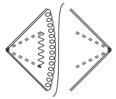
(a)

(b)

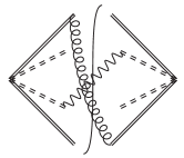
(c)

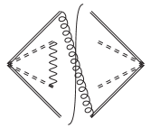
(d)

(e)

Figure 1: Feynman diagrams for the soft function at ${\cal O}(\alpha_{s}\alpha)$. Double solid lines stand for gluon Wilson lines, while double-dashed lines for photon Wilson lines. Corresponding conjugated and crossed diagrams should be added.

Let us start with the $D_{i}$ term, which can be calculated only from the soft function [60]. This is due to the fact that the $D_{i}$ term controls the evolution in the rapidity scale $\zeta$, which is a remnant of the arbitrary splitting of the soft function in rapidity space.

At leading order in $\alpha$, the $D_{i}$ term can be obtained from its analogous expression in pure QCD at order $\alpha_{s}$, since basically one needs to take the soft matrix element and calculate it at ${\cal O}(\alpha_{s}^{0}\alpha)$. The result is (see Appendix):

$$D_{i}^{(0,1)}(L_{\perp}) =\frac{\Gamma_{i}^{(0,1)}}{2}L_{\perp}\,,$$ (7)

where $\Gamma_{i}^{(0,1)}=4Q_{i}^{2}$, with $Q_{i}$ the fractional electric charge of the considered $i$ quark. We notice the flavor-dependence introduced by the QED corrections which, as already mentioned, breaks the flavor universality of the TMD evolution in pure QCD.

In order to obtain $D_{i}^{(1,1)}$, we realize that the soft function in perturbation theory in QCD$\times$QED can be written in a “factorized” form as

$$S_{i}(k_{sT})= \int\frac{d^{2}\mbox{\boldmath$y$}_{\perp}}{(2\pi)^{2}}e^{i\mbox{\boldmath${\scriptstyle y}$}_{\perp}\cdot\mbox{\boldmath${\scriptstyle k}$}_{s\perp}}\tilde{S}^{QCD}(y_{T})\,\tilde{S}_{i}^{QED}(y_{T})+{\cal O}(\alpha_{s}^{n}\alpha^{m})\Big{|}_{n\cdot m>1}\,,$$ (8)

where

$$\tilde{S}^{QCD}(y_{T})= \frac{{\rm Tr}_{c}}{N_{c}}\left<0\right|\left[S_{n}^{T\dagger}S_{\bar{n}}^{T}\right](0^{+},0^{-},\mbox{\boldmath$y$}_{\perp})\left[S^{T\dagger}_{\bar{n}}S_{n}^{T}\right](0)\left|0\right>\,,$$

$$\tilde{S}_{i}^{QED}(y_{T})= \left<0\right|\left[\widehat{S}_{i,n}^{T\dagger}\widehat{S}_{i,{\bar{n}}}^{T}\right](0^{+},0^{-},\mbox{\boldmath$y$}_{\perp})\left[\widehat{S}^{T\dagger}_{i,{\bar{n}}}\widehat{S}_{i,n}^{T}\right](0)\left|0\right>\,.$$ (9)

This factorized expression captures all contributions to the soft function at ${\cal O}(\alpha_{s}^{n}\alpha^{0})$ and ${\cal O}(\alpha_{s}^{0}\alpha^{n})$ for any $n$, and also the first mixed ones at ${\cal O}(\alpha_{s}\alpha)$. Notice that the latter come solely from the multiplication of the two factorized matrix elements $\tilde{S}^{QCD}$ and $\tilde{S}_{i}^{QED}$, because there is no contribution at this order which can come from an interaction between gluon and photon Wilson lines, as shown by the representative Feynman diagrams in fig. 1. At higher mixed orders in $\alpha_{s}$ and $\alpha$ however, there will indeed be some of the contributions which cannot be casted in the factorized expression above.

On the other hand, the soft function has a special structure in perturbation theory. In particular, using the $\delta$-regulator, it can be written to all orders in perturbation theory as [13, 17]

$$\hbox{ln}\tilde{S}_{i}(b_{T}) =A_{i}(L_{\perp};\alpha_{s},\alpha)+2D_{i}(L_{\perp};\alpha_{s},\alpha)\hbox{ln}\frac{\delta^{+}\delta^{-}}{\mu^{2}}\,,$$ (10)

where we have included also the QED corrections, $A_{i}$ is a generic function and $D_{i}$ the already introduced function which controls the rapidity evolution of TMDs. Combining this result with the expression in (8), it is easy to see that

$$D_{i}^{(1,1)}(L_{\perp}) =0\,.$$ (11)

(a)

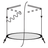
(b)

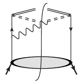
(c)

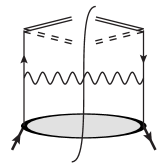
(d)

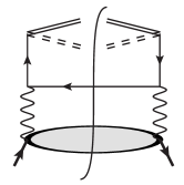
(e)

Figure 2: Feynman diagrams for the TMDPDF at ${\cal O}(\alpha_{s}^{0}\alpha)$. Double solid lines represent gluon Wilson lines, while double dashed lines stand for photon Wilson lines.

Finally, the $D_{i}$ term at ${\cal O}(\alpha^{2})$ can again be obtained from its analogous expression in QCD. The result is

$$D_{i}^{(0,2)}(L_{\perp}) =\frac{\Gamma_{i}^{(0,1)}}{4\widehat{\beta}^{(0,1)}}\left(\widehat{\beta}^{(0,1)}L_{\perp}\right)^{2}+\left(\frac{\Gamma_{i}^{(0,2)}}{2\widehat{\beta}^{(0,1)}}\right)\left(\widehat{\beta}^{(0,1)}L_{\perp}\right)+D_{i}^{(0,2)}(0)\,,$$ (12)

where (see appendix for $D^{(2,0)}(0)$ and $\Gamma^{(2,0)}$)

$$D_{i}^{(0,2)}(0) =-\left(\frac{112}{27}\right)Q_{i}^{2}\big{[}N_{c}\sum_{j}^{n_{f}}Q_{j}^{2}+n_{l}Q_{l}^{2}\big{]}\,,$$

$$\Gamma_{i}^{(0,2)}/\Gamma_{i}^{(0,1)} =-\frac{20}{9}\big{[}N_{c}\sum_{j}^{n_{f}}Q_{j}^{2}+n_{l}Q_{l}^{2}\big{]}\,,$$ (13)

where $Q_{j}$ is the fractional charge of the active quarks ($n_{f}$) and $Q_{l}=1$ the one of the active leptons ($n_{l}$) in a fermion loop. We need as well the QCD and QED $\beta$ functions and the mixed contributions at ${\cal O}(\alpha_{s}\alpha)$:

$$\frac{d\hbox{ln}\alpha_{s}}{d\hbox{ln}\mu^{2}} \equiv\beta\big{(}\alpha_{s}(\mu),\alpha(\mu)\big{)}=-\sum_{n,m}\beta^{(n,m)}\left(\frac{\alpha_{s}}{4\pi}\right)^{n}\left(\frac{\alpha}{4\pi}\right)^{m}\,,$$ (14)

$$\frac{d\hbox{ln}\alpha}{d\hbox{ln}\mu^{2}} \equiv\widehat{\beta}\big{(}\alpha_{s}(\mu),\alpha(\mu)\big{)}=-\sum_{n,m}\widehat{\beta}^{(n,m)}\left(\frac{\alpha_{s}}{4\pi}\right)^{n}\left(\frac{\alpha}{4\pi}\right)^{m}\,,$$ (15)

with the coefficients (see e.g. [61, 62])

$$\beta^{(1,1)} =-2\sum_{j}^{n_{f}}Q_{j}^{2}\,,$$ (16)

$$\widehat{\beta}^{(0,1)} =-\frac{4}{3}\big{[}N_{c}\sum_{j}^{n_{f}}Q_{j}^{2}+n_{l}Q_{l}^{2}\big{]}\,,$$ (17)

$$\widehat{\beta}^{(0,2)} =-4\big{[}N_{c}\sum_{j}^{n_{f}}Q_{j}^{4}+n_{l}Q_{l}^{4}\big{]}\,,$$ (18)

$$\widehat{\beta}^{(1,1)} =-4C_{F}N_{c}\sum_{j}^{n_{f}}Q_{j}^{2}\,.$$ (19)

We turn now to the QED corrections to the anomalous dimension $\gamma_{F_{i}}$. At leading order in $\alpha$, the anomalous dimension is calculated from the virtual diagrams in figs. 2a-2b, together with the corresponding one-loop diagram of the soft function in pure QED, and apart from charge factors, it has an analogous expression to that in QCD. The result is:

$$\gamma_{i}^{(0,1)} =-6Q_{i}^{2}\,,$$

$$\Gamma_{i}^{(0,1)} =4Q_{i}^{2}\,.$$ (20)

At ${\cal O}(\alpha_{s}\alpha)$ one can take the results $\gamma_{i}^{(0,2)}$ and $\Gamma_{i}^{(0,2)}$ from the appendix and apply the recipe to translate QCD color factors to QED charge factors. In this case, one needs to replace one gluon by one photon in the two-gluon diagrams that contribute in pure QCD. Proceeding in this way we obtain

$$\gamma_{i}^{(1,1)} =2C_{F}Q_{i}^{2}\left(-3+4\pi^{2}-48\zeta_{3}\right)\,,$$

$$\Gamma_{i}^{(1,1)} =0\,.$$ (21)

In order to obtain $\gamma_{i}^{(1,1)}$, we have noted that by color/charge conservation there cannot be fermion-loop diagrams at ${\cal O}(\alpha_{s}\alpha)$, nor in the collinear matrix element $J_{i/P}$ nor in the soft function (see fig. 1), so the term proportional to $T_{F}n_{f}$ in $\gamma_{i}^{(0,2)}$ (see Appendix) does not contribute after taking the (partial) Abelian limit. In fact, only the diagrams in figs. 3a and 3b (and similar ones) and the ones in fig. 1 contribute. Also, we added an additional factor of 2 to $\gamma_{i}^{(1,1)}$ as compared to $\gamma_{i}^{(2,0)}$, since there are two ways of replacing the 2 internal gluons in the relevant Feynman diagrams by a gluon and a photon. We note that in [61, 62] it is also found that $\Gamma_{i}^{(1,1)}=0$.

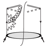
(a)

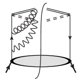
(b)

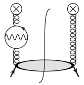
(c)

Figure 3: (a)-(b): representative Feynman diagrams which contribute to $\gamma_{F_{i}}$ for quark TMDs at ${\cal O}(\alpha_{s}\alpha)$ through $J_{i/P}$. (c): similar but for $\gamma_{F_{g}}$ for gluon TMDs, where the crossed vertex stands for the collinear gluon Wilson line in $J_{g/P}$.

Finally, we provide the two-loop QED corrections to the anomalous dimension $\gamma_{F_{i}}$. Again, they can be obtained from the expressions in pure QCD $\gamma_{i}^{(2,0)}$ and $\Gamma_{i}^{(2,0)}$, by replacing in the relevant Feynman diagrams the two gluons by two photons. The results are:

$$\gamma_{i}^{(0,2)} =Q_{i}^{4}\left(-3+4\pi^{2}-48\zeta_{3}\right)$$

$$+Q_{i}^{2}\big{[}N_{c}\sum_{j}^{n_{f}}Q_{j}^{2}+n_{l}Q_{l}^{2}\big{]}\left(\frac{260}{27}+\frac{4\pi^{2}}{3}\right)\,,$$

$$\Gamma_{i}^{(0,2)}/\Gamma_{i}^{(0,1)} =-\frac{20}{9}\big{[}N_{c}\sum_{j}^{n_{f}}Q_{j}^{2}+n_{l}Q_{l}^{2}\big{]}\,.$$ (22)

Now we turn our attention to the evolution kernel for gluon TMDs [54], which is analogous to the one of quark TMDs shown at the beginning of this section in (3) with $i=g$. The QED corrections to the relevant anomalous dimension $\gamma_{F_{g}}$ and the $D_{g}$ term only appear, however, at ${\cal O}(\alpha_{s}\alpha)$ and beyond, and there are no pure QED corrections. This is because, given color/charge conservation, one needs in the relevant Feynman diagrams at least one closed quark loop, where a gluon inside can be replaced by a photon. In fact, only the collinear matrix element $J_{g/P}$ contributes at ${\cal O}(\alpha_{s}\alpha)$, see fig. 3c, since the soft function for gluon TMDs starts to contribute at ${\cal O}(\alpha_{s}^{2}\alpha)$.

The non-cusp anomalous dimension for gluon TMDs in pure QCD at ${\cal O}(\alpha_{s}^{2})$ is (see e.g. [54])

$$\gamma_{g}^{(2,0)} =2C_{A}^{2}\left(-\frac{692}{27}+\frac{11\pi^{2}}{18}+2\zeta_{3}\right)+2C_{A}T_{F}n_{f}\left(\frac{256}{27}-\frac{2\pi^{2}}{9}\right)$$

$$+8C_{F}T_{F}n_{f}\,,$$ (23)

from which we obtain

$$\gamma_{g}^{(1,1)} =8T_{F}\sum_{j}^{n_{f}}Q_{j}^{2}\,.$$ (24)

Notice that there is no factor $N_{c}$, because we are replacing an inner gluon by a photon in a closed fermion loop inside a gluon line, which remains. Thus we do not need to account for the color multiplicity, as in the case of a fermion loop inside a photon line.

The cusp anomalous dimension for gluons does not receive QED corrections at ${\cal O}(\alpha_{s}\alpha)$: $\Gamma_{g}^{(1,1)}=0$. Neither does the $D^{g}$ term, since the soft function (for gluon TMDs) from which it can be obtained is zero at this order, and thus $D_{g}^{(1,1)}=0$.

4 QED corrections for $f_{1}$ at large transverse momentum

When the transverse momentum is large, i.e. the impact parameter is small, the unpolarized quark TMDPDF can be expanded through an operator product expansion (OPE) in terms of its corresponding integrated counterparts, the collinear quark/gluon PDFs:

$${\tilde{f}}_{i/A}(x,b_{T};\zeta,\mu) =\sum_{j=q,\bar{q},g,\gamma}{\tilde{C}}_{i/j}(x,b_{T};\zeta,\mu)\otimes f_{j/A}(x;\mu)\,$$

$$+{\cal O}\Big{(}b_{T}\Lambda_{\rm QCD}\Big{)}\,,$$ (25)

where $\zeta_{0}\sim\mu_{0}^{2}\sim\mu_{b}^{2}$, with $\mu_{b}=2e^{-\gamma_{E}}/b_{T}$ the natural scale at which the OPE is performed. Notice that we have included the contribution of the photon PDF in the OPE. The coefficients $\tilde{C}_{i/j}$ (excluding $j=\gamma$, which is part of the aim of this paper) are currently known in pure QCD up to ${\cal O}(\alpha_{s}^{2})$ (see e.g. [22]).

We consider the inclusion of the QED corrections at LO, which will modify the evolution/resummation of the TMDPDF. As already discussed, they will contribute to the evolution of the TMDs. In addition, they will affect the matching of the TMDPDF onto its collinear counterparts.

The photon PDF will have to be included in the sum over partons of the OPE, as introduced above. This will amount to have a matching coefficient of the quark TMDPDF onto the photon PDF, which is:

$${\tilde{C}}_{i/\gamma}^{(0,1)}(x,b_{T};\mu) =N_{c}Q_{i}^{2}\Big{[}-2L_{T}\big{(}x^{2}+(1-x)^{2}\big{)}+4x(1-x)\Big{]}\,.$$ (26)

This coefficient can be calculated directly by an explicit perturbative calculation of both the quark TMDPDF and the photon PDF (by subtraction using (4)), or obtained for instance from ${\tilde{C}}_{i/g}^{(1,0)}$ in eq. (39) in [7] or eq. (A10) in [11] by replacing the color factor ($T_{F}$) by the proper charge factor ($N_{c}Q_{i}^{2}$). Notice that we have included a factor $N_{c}$, which accounts for the color multiplicity of the quark .

Also the matching coefficient of the TMDPDF onto the quark PDF will have to be modified, which at ${\cal O}(\alpha)$ is analogous to the pure QCD one ${\tilde{C}}_{i/i}^{(1,0)}$. In fact, one has:

$${\tilde{C}}_{i/i}^{(0,1)}(x,b_{T};\mu) =Q_{i}^{2}\Bigg{[}\delta(1-x)\left(-L_{T}^{2}+3L_{T}+2L_{T}\hbox{ln}\frac{\mu^{2}}{Q^{2}}-\frac{\pi^{2}}{6}\right)$$

$$-2L_{T}{\cal P}_{i\leftarrow i}+2(1-x)\Bigg{]}\,.$$ (27)

This can also be directly calculated by considering the quark TMDPDF and the quark PDF up to ${\cal O}(\alpha)$. The inclusion of the newly derived coefficients ${\tilde{C}}_{i/i}^{(0,1)}$ and ${\tilde{C}}_{i/\gamma}^{(0,1)}$ will be necessary at N³LL and beyond, if one takes the recipe in table 1 with the counting $\alpha\sim\alpha_{s}^{2}$. The QED corrections to the OPE coefficients at ${\cal O}(\alpha_{s}\alpha)$, even if possible to derive from the already known ones at ${\cal O}(\alpha_{s}^{2})$ in pure QCD, will only enter at N⁴LL, which is far beyond the current achievable theoretical precision, and even more of the experimental one.

We end this section by noting that the leading-order QED corrections to the OPE coefficients of the helicity and transversity TMDPDFs and the unpolarized, helicity and transversity TMDFFs can be calculated similarly, starting from the known expressions in pure QCD. Also the ones corresponding to polarized TMDs, as the Sivers or Collins functions. We leave this for a future effort.

5 Conclusions

By extending the operator definition of TMDs from pure QCD to QCD$\times$QED, we have calculated the mixed corrections to the relevant anomalous dimensions at ${\cal O}(\alpha_{s}\alpha)$ and the pure QED ones up to ${\cal O}(\alpha^{2})$. They apply to all the leading-twist unpolarized and polarized quark and gluon TMD parton distribution and fragmentation functions. To do so, we have taken advantage of the known results in pure QCD at ${\cal O}(\alpha_{s}^{2})$ and replaced, in the relevant Feynman diagrams, one internal gluon by a photon, or two gluons by two photons, and then recalculated the proper color/charge factors. These corrections depend on the flavor of the considered parton, and thus break the full flavor universality of the TMD evolution kernel in pure QCD (but not the spin universality).

In addition, we have also calculated the leading-order QED corrections at ${\cal O}(\alpha)$ to the matching coefficients of the unpolarized quark TMDPDF onto its integrated counterparts, again profiting from known results in pure QCD. Following the same procedure, the analogous QED corrections to other TMDs can be calculated in a straightforward way.

The newly calculated corrections will make it possible to perform very precise resummations of large logarithms for any of the leading-twist TMDs, in view of the precision needs of future planned experiments [40, 41, 42, 43, 44].

Finally, we note that the new results apply as well to the evolution of generalized TMDs, since their evolution is analogous to the one of the TMDs [63].

Acknowledgements. We thank Joan Soto for his contributions to the initial stage of this project. AB and MGE are supported by the European Research Council (ERC) under the European Union’s Horizon 2020 research and innovation program (grant agreement No. 647981, 3DSPIN). MGE is supported by the Marie Skłodowska-Curie grant GlueCore (grant agreement No. 793896).

Appendix A Anomalous dimensions

The cusp anomalous dimension $\Gamma$ is:

$$\Gamma^{(1,0)} =4C_{F}\,,$$

$$\Gamma^{(2,0)}/\Gamma^{(1,0)} =\left(\frac{67}{9}-\frac{\pi^{2}}{3}\right)C_{A}-\frac{20}{9}T_{F}n_{f}\,,$$

$$\Gamma^{(3,0)}/\Gamma^{(1,0)} =C_{A}^{2}\left(\frac{245}{6}-\frac{134\pi^{2}}{27}+\frac{11\pi^{4}}{45}+\frac{22}{3}\,\zeta_{3}\right)$$

$$+C_{A}T_{F}n_{f}\left(-\frac{418}{27}+\frac{40\pi^{2}}{27}-\frac{56}{3}\,\zeta_{3}\right)$$

$$+C_{F}T_{F}n_{f}\left(-\frac{55}{3}+16\zeta_{3}\right)-\frac{16}{27}\,T_{F}^{2}n_{f}^{2}\,.$$ (28)

The non-cusp anomalous dimension $\gamma$:

$$\gamma^{(1,0)} =-6C_{F},$$

$$\gamma^{(2,0)} =C_{F}^{2}\left(-3+4\pi^{2}-48\zeta_{3}\right)+C_{F}C_{A}\left(-\frac{961}{27}-\frac{11\pi^{2}}{3}+52\zeta_{3}\right)$$

$$+C_{F}T_{F}n_{f}\left(\frac{260}{27}+\frac{4\pi^{2}}{3}\right),$$ (29)

$$\gamma^{(3,0)} =C_{F}^{3}\left(-29-6\pi^{2}-\frac{16\pi^{4}}{5}-136\zeta_{3}+\frac{32\pi^{2}}{3}\,\zeta_{3}+480\zeta_{5}\right)$$

$$+C_{F}^{2}C_{A}\Bigg{(}-\frac{151}{2}+\frac{410\pi^{2}}{9}+\frac{494\pi^{4}}{135}-\frac{1688}{3}\,\zeta_{3}$$

$$-\frac{16\pi^{2}}{3}\,\zeta_{3}-240\zeta_{5}\Bigg{)}$$

$$+C_{F}C_{A}^{2}\Bigg{(}-\frac{139345}{1458}-\frac{7163\pi^{2}}{243}-\frac{83\pi^{4}}{45}+\frac{7052}{9}\,\zeta_{3}$$

$$-\frac{88\pi^{2}}{9}\,\zeta_{3}-272\zeta_{5}\Bigg{)}$$

$$+C_{F}^{2}T_{F}n_{f}\left(\frac{5906}{27}-\frac{52\pi^{2}}{9}-\frac{56\pi^{4}}{27}+\frac{1024}{9}\,\zeta_{3}\right)$$

$$+C_{F}C_{A}T_{F}n_{f}\left(-\frac{34636}{729}+\frac{5188\pi^{2}}{243}+\frac{44\pi^{4}}{45}-\frac{3856}{27}\,\zeta_{3}\right)$$

$$+C_{F}T_{F}^{2}n_{f}^{2}\left(\frac{19336}{729}-\frac{80\pi^{2}}{27}-\frac{64}{27}\,\zeta_{3}\right)\,.$$ (30)

The coefficients of the $D$ term are

$$D^{(1,0)}(L_{\perp}) =\frac{\Gamma^{(1,0)}}{2\beta^{(1,0)}}\left(\beta^{(1,0)}L_{\perp}\right)+D^{(1,0)}(0)\,,$$

$$D^{(2,0)}(L_{\perp}) =\frac{\Gamma^{(1,0)}}{4\beta^{(1,0)}}\left(\beta^{(1,0)}L_{\perp}\right)^{2}+\left(\frac{\Gamma^{(2,0)}}{2\beta^{(1,0)}}+D^{(1,0)}(0)\right)\big{(}\beta^{(1,0)}L_{\perp}\big{)}$$

$$+D^{(2,0)}(0)\,,$$

$$D^{(3,0)}(L_{\perp}) =\frac{\Gamma^{(1,0)}}{6\beta^{(1,0)}}\left(\beta^{(1,0)}L_{\perp}\right)^{3}$$

$$+\frac{1}{2}\left(\frac{\Gamma^{(2,0)}}{\beta^{(1,0)}}+\frac{1}{2}\frac{\Gamma^{(1,0)}\beta^{(2,0)}}{[\beta^{(1,0)}]^{2}}+2D^{(1,0)}(0)\right)\left(\beta^{(1,0)}L_{\perp}\right)^{2}$$

$$+\frac{1}{2}\left(4D^{(2,0)}(0)+\frac{\beta^{(2,0)}}{\beta^{(1,0)}}2D^{(1,0)}(0)+\frac{\Gamma^{(3,0)}}{\beta^{(1,0)}}\right)\left(\beta^{(1,0)}L_{\perp}\right)$$

$$+D^{(3,0)}(0)\,,$$ (31)

with $L_{\perp}=\hbox{ln}\frac{\mu^{2}b^{2}}{4e^{-2\gamma_{E}}}$ and

$$D^{(1,0)}(0) =0\,,$$

$$D^{(2,0)}(0) =C_{F}C_{A}\left(\frac{404}{27}-14\zeta_{3}\right)-\left(\frac{112}{27}\right)C_{F}T_{F}n_{f}\,,$$

$$D^{(3,0)}(0) =\frac{-1}{2}C_{F}C_{A}^{2}\Bigg{(}-\frac{176}{3}\zeta_{3}\zeta_{2}+\frac{6392\zeta_{2}}{81}+\frac{12328\zeta_{3}}{27}$$

$$+\frac{154\zeta_{4}}{3}-192\zeta_{5}-\frac{297029}{729}\Bigg{)}$$

$$-C_{F}C_{A}T_{F}n_{f}\left(-\frac{824\zeta_{2}}{81}-\frac{904\zeta_{3}}{27}+\frac{20\zeta_{4}}{3}+\frac{62626}{729}\right)$$

$$-2T_{F}^{2}n_{f}^{2}\left(-\frac{32\zeta_{3}}{9}-\frac{1856}{729}\right)$$

$$-C_{F}^{2}T_{F}n_{f}\left(\frac{-304\zeta_{3}}{9}-16\zeta_{4}+\frac{1711}{27}\right)\,.$$ (32)

The result for $D^{(3,0)}(0)$ has been recently computed in [18]. The rest can be found also in [15].

Finally, the coefficients for the QCD $\beta$-function are

$$\beta^{(1,0)} =\frac{11}{3}\,C_{A}-\frac{4}{3}\,T_{F}n_{f}\,,$$

$$\beta^{(2,0)} =\frac{34}{3}\,C_{A}^{2}-\frac{20}{3}\,C_{A}T_{F}n_{f}-4C_{F}T_{F}n_{f}\,,$$

$$\beta^{(3,0)} =\frac{2857}{54}\,C_{A}^{3}+\left(2C_{F}^{2}-\frac{205}{9}\,C_{F}C_{A}-\frac{1415}{27}\,C_{A}^{2}\right)T_{F}n_{f}$$

$$+\left(\frac{44}{9}\,C_{F}+\frac{158}{27}\,C_{A}\right)T_{F}^{2}n_{f}^{2}\,,$$

$$\beta^{(4,0)} =\frac{149753}{6}+3564\zeta_{3}-\left(\frac{1078361}{162}+\frac{6508}{27}\,\zeta_{3}\right)n_{f}$$

$$+\left(\frac{50065}{162}+\frac{6472}{81}\,\zeta_{3}\right)n_{f}^{2}+\frac{1093}{729}\,n_{f}^{3}\,,$$ (33)

where for $\beta^{(4,0)}$ we have used $N_{c}=3$ and $T_{F}=\frac{1}{2}$.

References

- [1] R. Angeles-Martinez et al., “Transverse Momentum Dependent (TMD) parton distribution functions: status and prospects,” Acta Phys. Polon. B46 no. 12, (2015) 2501–2534, arXiv:1507.05267 [hep-ph].
- [2] T. C. Rogers, “An overview of transverse-momentum-dependent factorization and evolution,” Eur. Phys. J. A52 no. 6, (2016) 153, arXiv:1509.04766 [hep-ph].
- [3] M. Diehl, “Introduction to GPDs and TMDs,” Eur. Phys. J. A52 no. 6, (2016) 149, arXiv:1512.01328 [hep-ph].
- [4] X.-d. Ji, J.-p. Ma, and F. Yuan, “QCD factorization for semi-inclusive deep-inelastic scattering at low transverse momentum,” Phys. Rev. D71 (2005) 034005, arXiv:hep-ph/0404183 [hep-ph].
- [5] J. Collins and J.-W. Qiu, “ factorization is violated in production of high-transverse-momentum particles in hadron-hadron collisions,” Phys. Rev. D75 (2007) 114014, arXiv:0705.2141 [hep-ph].
- [6] T. C. Rogers and P. J. Mulders, “No Generalized TMD-Factorization in Hadro-Production of High Transverse Momentum Hadrons,” Phys. Rev. D81 (2010) 094006, arXiv:1001.2977 [hep-ph].
- [7] T. Becher and M. Neubert, “Drell-Yan Production at Small , Transverse Parton Distributions and the Collinear Anomaly,” Eur. Phys. J. C71 (2011) 1665, arXiv:1007.4005 [hep-ph].
- [8] J.-Y. Chiu, A. Jain, D. Neill, and I. Z. Rothstein, “A Formalism for the Systematic Treatment of Rapidity Logarithms in Quantum Field Theory,” JHEP 05 (2012) 084, arXiv:1202.0814 [hep-ph].
- [9] S. Mantry and F. Petriello, “Transverse Momentum Distributions in the Non-Perturbative Region,” Phys. Rev. D84 (2011) 014030, arXiv:1011.0757 [hep-ph].
- [10] J. Collins, “Foundations of perturbative QCD,” Camb. Monogr. Part. Phys. Nucl. Phys. Cosmol. 32 (2011) 1–624.
- [11] S. M. Aybat and T. C. Rogers, “TMD Parton Distribution and Fragmentation Functions with QCD Evolution,” Phys. Rev. D83 (2011) 114042, arXiv:1101.5057 [hep-ph].
- [12] M. G. Echevarria, A. Idilbi, and I. Scimemi, “Factorization Theorem For Drell-Yan At Low And Transverse Momentum Distributions On-The-Light-Cone,” JHEP 07 (2012) 002, arXiv:1111.4996 [hep-ph].
- [13] M. G. Echevarria, A. Idilbi, and I. Scimemi, “Soft and Collinear Factorization and Transverse Momentum Dependent Parton Distribution Functions,” Phys. Lett. B726 (2013) 795–801, arXiv:1211.1947 [hep-ph].
- [14] A. Vladimirov, “Structure of rapidity divergences in multi-parton scattering soft factors,” JHEP 04 (2018) 045, arXiv:1707.07606 [hep-ph].
- [15] M. G. Echevarria, A. Idilbi, A. Schaefer, and I. Scimemi, “Model-Independent Evolution of Transverse Momentum Dependent Distribution Functions (TMDs) at NNLL,” Eur. Phys. J. C73 no. 12, (2013) 2636, arXiv:1208.1281 [hep-ph].
- [16] M. G. Echevarria, A. Idilbi, and I. Scimemi, “Unified treatment of the QCD evolution of all (un-)polarized transverse momentum dependent functions: Collins function as a study case,” Phys. Rev. D90 no. 1, (2014) 014003, arXiv:1402.0869 [hep-ph].
- [17] M. G. Echevarria, I. Scimemi, and A. Vladimirov, “Universal transverse momentum dependent soft function at NNLO,” Phys. Rev. D93 no. 5, (2016) 054004, arXiv:1511.05590 [hep-ph].
- [18] Y. Li and H. X. Zhu, “Bootstrapping Rapidity Anomalous Dimensions for Transverse-Momentum Resummation,” Phys. Rev. Lett. 118 no. 2, (2017) 022004, arXiv:1604.01404 [hep-ph].
- [19] A. A. Vladimirov, “Correspondence between Soft and Rapidity Anomalous Dimensions,” Phys. Rev. Lett. 118 no. 6, (2017) 062001, arXiv:1610.05791 [hep-ph].
- [20] S. Catani, L. Cieri, D. de Florian, G. Ferrera, and M. Grazzini, “Universality of transverse-momentum resummation and hard factors at the NNLO,” Nucl. Phys. B881 (2014) 414–443, arXiv:1311.1654 [hep-ph].
- [21] T. Gehrmann, T. Luebbert, and L. L. Yang, “Calculation of the transverse parton distribution functions at next-to-next-to-leading order,” JHEP 06 (2014) 155, arXiv:1403.6451 [hep-ph].
- [22] M. G. Echevarria, I. Scimemi, and A. Vladimirov, “Unpolarized Transverse Momentum Dependent Parton Distribution and Fragmentation Functions at next-to-next-to-leading order,” JHEP 09 (2016) 004, arXiv:1604.07869 [hep-ph].
- [23] A. Bacchetta and A. Prokudin, “Evolution of the helicity and transversity Transverse-Momentum-Dependent parton distributions,” Nucl. Phys. B875 (2013) 536–551, arXiv:1303.2129 [hep-ph].
- [24] D. Gutiérrez-Reyes, I. Scimemi, and A. A. Vladimirov, “Twist-2 matching of transverse momentum dependent distributions,” Phys. Lett. B769 (2017) 84–89, arXiv:1702.06558 [hep-ph].
- [25] M. G. A. Buffing, M. Diehl, and T. Kasemets, “Transverse momentum in double parton scattering: factorisation, evolution and matching,” JHEP 01 (2018) 044, arXiv:1708.03528 [hep-ph].
- [26] D. Gutierrez-Reyes, I. Scimemi, and A. Vladimirov, “Transverse momentum dependent transversely polarized distributions at next-to-next-to-leading-order,” arXiv:1805.07243 [hep-ph].
- [27] M. G. Echevarria, A. Idilbi, Z.-B. Kang, and I. Vitev, “QCD Evolution of the Sivers Asymmetry,” Phys. Rev. D89 (2014) 074013, arXiv:1401.5078 [hep-ph].
- [28] U. D’Alesio, M. G. Echevarria, S. Melis, and I. Scimemi, “Non-perturbative QCD effects in spectra of Drell-Yan and Z-boson production,” JHEP 11 (2014) 098, arXiv:1407.3311 [hep-ph].
- [29] A. Bacchetta, F. Delcarro, C. Pisano, M. Radici, and A. Signori, “Extraction of partonic transverse momentum distributions from semi-inclusive deep-inelastic scattering, Drell-Yan and Z-boson production,” JHEP 06 (2017) 081, arXiv:1703.10157 [hep-ph].
- [30] I. Scimemi and A. Vladimirov, “Analysis of vector boson production within TMD factorization,” Eur. Phys. J. C78 no. 2, (2018) 89, arXiv:1706.01473 [hep-ph].
- [31] S. M. Aybat, A. Prokudin, and T. C. Rogers, “Calculation of TMD Evolution for Transverse Single Spin Asymmetry Measurements,” Phys. Rev. Lett. 108 (2012) 242003, arXiv:1112.4423 [hep-ph].
- [32] M. Anselmino, M. Boglione, and S. Melis, “A Strategy towards the extraction of the Sivers function with TMD evolution,” Phys. Rev. D86 (2012) 014028, arXiv:1204.1239 [hep-ph].
- [33] Z.-B. Kang, A. Prokudin, P. Sun, and F. Yuan, “Extraction of Quark Transversity Distribution and Collins Fragmentation Functions with QCD Evolution,” Phys. Rev. D93 no. 1, (2016) 014009, arXiv:1505.05589 [hep-ph].
- [34] ATLAS Collaboration, G. Aad et al., “Measurement of the boson transverse momentum distribution in collisions at = 7 TeV with the ATLAS detector,” JHEP 09 (2014) 145, arXiv:1406.3660 [hep-ex].
- [35] ATLAS Collaboration, G. Aad et al., “Measurement of the transverse momentum and distributions of Drell-Yan lepton pairs in proton-proton collisions at TeV with the ATLAS detector,” Eur. Phys. J. C76 no. 5, (2016) 291, arXiv:1512.02192 [hep-ex].
- [36] LHCb Collaboration, R. Aaij et al., “Measurement of the forward boson production cross-section in collisions at TeV,” JHEP 08 (2015) 039, arXiv:1505.07024 [hep-ex].
- [37] LHCb Collaboration, R. Aaij et al., “Measurement of forward W and Z boson production in collisions at TeV,” JHEP 01 (2016) 155, arXiv:1511.08039 [hep-ex].
- [38] LHCb Collaboration, R. Aaij et al., “Measurement of the forward Z boson production cross-section in pp collisions at TeV,” JHEP 09 (2016) 136, arXiv:1607.06495 [hep-ex].
- [39] CMS Collaboration, V. Khachatryan et al., “Measurement of the transverse momentum spectra of weak vector bosons produced in proton-proton collisions at TeV,” JHEP 02 (2017) 096, arXiv:1606.05864 [hep-ex].
- [40] A. Accardi et al., “Electron Ion Collider: The Next QCD Frontier,” Eur. Phys. J. A52 no. 9, (2016) 268, arXiv:1212.1701 [nucl-ex].
- [41] J. Dudek et al., “Physics Opportunities with the 12 GeV Upgrade at Jefferson Lab,” Eur. Phys. J. A48 (2012) 187, arXiv:1208.1244 [hep-ex].
- [42] S. J. Brodsky, F. Fleuret, C. Hadjidakis, and J. P. Lansberg, “Physics Opportunities of a Fixed-Target Experiment using the LHC Beams,” Phys. Rept. 522 (2013) 239–255, arXiv:1202.6585 [hep-ph].
- [43] D. Kikola, M. G. Echevarria, C. Hadjidakis, J.-P. Lansberg, C. Lorcé, L. Massacrier, C. M. Quintans, A. Signori, and B. Trzeciak, “Feasibility Studies for Single Transverse-Spin Asymmetry Measurements at a Fixed-Target Experiment Using the LHC Proton and Lead Beams (AFTER@LHC),” Few Body Syst. 58 no. 4, (2017) 139, arXiv:1702.01546 [hep-ex].
- [44] C. Hadjidakis et al., “A Fixed-Target Programme at the LHC: Physics Case and Projected Performances for Heavy-Ion, Hadron, Spin and Astroparticle Studies,” arXiv:1807.00603 [hep-ex].
- [45] M. Roth and S. Weinzierl, “QED corrections to the evolution of parton distributions,” Phys. Lett. B590 (2004) 190–198, arXiv:hep-ph/0403200 [hep-ph].
- [46] A. D. Martin, R. G. Roberts, W. J. Stirling, and R. S. Thorne, “Parton distributions incorporating QED contributions,” Eur. Phys. J. C39 (2005) 155–161, arXiv:hep-ph/0411040 [hep-ph].
- [47] NNPDF Collaboration, R. D. Ball, V. Bertone, S. Carrazza, L. Del Debbio, S. Forte, A. Guffanti, N. P. Hartland, and J. Rojo, “Parton distributions with QED corrections,” Nucl. Phys. B877 (2013) 290–320, arXiv:1308.0598 [hep-ph].
- [48] D. de Florian, G. F. R. Sborlini, and G. Rodrigo, “QED corrections to the Altarelli-Parisi splitting functions,” Eur. Phys. J. C76 no. 5, (2016) 282, arXiv:1512.00612 [hep-ph].
- [49] D. de Florian, G. F. R. Sborlini, and G. Rodrigo, “Two-loop QED corrections to the Altarelli-Parisi splitting functions,” JHEP 10 (2016) 056, arXiv:1606.02887 [hep-ph].
- [50] M. Mottaghizadeh, F. Taghavi Shahri, and P. Eslami, “Analytical solutions of the QEDQCD DGLAP evolution equations based on the Mellin transform technique,” Phys. Lett. B773 (2017) 375–384, arXiv:1707.00108 [hep-ph].
- [51] D. de Florian, M. Der, and I. Fabre, “QCDQED NNLO corrections to Drell Yan production,” arXiv:1805.12214 [hep-ph].
- [52] L. Cieri, G. Ferrera, and G. F. R. Sborlini, “Combining QED and QCD transverse-momentum resummation for Z boson production at hadron colliders,” arXiv:1805.11948 [hep-ph].
- [53] M. Garcia-Echevarria, A. Idilbi, and I. Scimemi, “SCET, Light-Cone Gauge and the T-Wilson Lines,” Phys. Rev. D84 (2011) 011502, arXiv:1104.0686 [hep-ph].
- [54] M. G. Echevarria, T. Kasemets, P. J. Mulders, and C. Pisano, “QCD evolution of (un)polarized gluon TMDPDFs and the Higgs -distribution,” JHEP 07 (2015) 158, arXiv:1502.05354 [hep-ph]. [Erratum: JHEP05,073(2017)].
- [55] S. Moch, J. A. M. Vermaseren, and A. Vogt, “The Quark form-factor at higher orders,” JHEP 08 (2005) 049, arXiv:hep-ph/0507039 [hep-ph].
- [56] S. Moch, J. A. M. Vermaseren, and A. Vogt, “The Three loop splitting functions in QCD: The Nonsinglet case,” Nucl. Phys. B688 (2004) 101–134, arXiv:hep-ph/0403192 [hep-ph].
- [57] S. Moch, B. Ruijl, T. Ueda, J. A. M. Vermaseren, and A. Vogt, “Four-Loop Non-Singlet Splitting Functions in the Planar Limit and Beyond,” JHEP 10 (2017) 041, arXiv:1707.08315 [hep-ph].
- [58] J. Collins and T. Rogers, “Understanding the large-distance behavior of transverse-momentum-dependent parton densities and the Collins-Soper evolution kernel,” Phys. Rev. D91 no. 7, (2015) 074020, arXiv:1412.3820 [hep-ph].
- [59] I. Scimemi and A. Vladimirov, “Systematic analysis of double-scale evolution,” arXiv:1803.11089 [hep-ph].
- [60] M. G. Echevarria, I. Scimemi, and A. Vladimirov, “Transverse momentum dependent fragmentation function at next-to–next-to–leading order,” Phys. Rev. D93 no. 1, (2016) 011502, arXiv:1509.06392 [hep-ph]. [Erratum: Phys. Rev.D94,no.9,099904(2016)].
- [61] W. B. Kilgore and C. Sturm, “Two-Loop Virtual Corrections to Drell-Yan Production at order ,” Phys. Rev. D85 (2012) 033005, arXiv:1107.4798 [hep-ph].
- [62] W. B. Kilgore, “The Two-Loop Infrared Structure of Amplitudes with Mixed Gauge Groups,” Eur. Phys. J. C73 (2013) 2603, arXiv:1308.1055 [hep-ph].
- [63] M. G. Echevarria, A. Idilbi, K. Kanazawa, C. Lorcé, A. Metz, B. Pasquini, and M. Schlegel, “Proper definition and evolution of generalized transverse momentum dependent distributions,” Phys. Lett. B759 (2016) 336–341, arXiv:1602.06953 [hep-ph].