Unitarity bound violation in holography and the Instability toward the Charge Density Wave

Abstract

We study the spectral function of holographic fermions with Pauli term and find that when bulk mass goes beyond the unitarity bound there is an instability with tachyonic dispersion relation. Based on the the linear density dependence of wave vector involved, we suggest that the instability is toward the charge density wave(CDW) whose wave vector can be read off from the position of the tip of k-gap. We point out the similarity between the unitarity violation in this model and the ’Nesting’ as a mechanism of CDW.

1 Introduction

Instability of a theory is the indication that the physical system is not described by the correct degrees of freedom in the parameter regime it happens. It also plays a role of a messenger telling us that a new phase is ready there. The simplest example is the interacting scalar theory with its potential term $V[\phi]=r\phi^{2}$. For $r<0$, the fluctuation around $\phi=0$ is tachyonic one, leading to an instability. The system develops a new vacuum and the prescription to the symptom is to add $\phi^{4}$ term to $V[\phi]$ by considering higher interaction. In a conformally invariant system, one of the stability requirement is the conformal unitarity bound. Often the unitarity violation is associated with the presence of the ‘tachyon’, signaling an instability, which is natural because unitarity violation means that the degrees of freedom is sinking or emerging rather than being conserved. In fact, whenever a phase transition happens, physics is described by a new degree of freedom which is not given in the original hamiltonian. Also going from UV to IR fixed point is not a unitary process as the c-theorem of CFT says. At the level of the effective theory the old degrees of freedom were destroyed and new degrees of freedom were created around the phase transition point, therefore in a sense unitarity is doubly violated there. Therefore it is valuable to intentionally violate the unitarity bound to see what is going beyond the regime and try to get information about the new phase. Often it gives us useful information on the nature of the instability and the character of the new vacuum.

On the other hand, understanding the mechanism of CDW in strongly interacting system attracted much attentionWHANGBO_1991 ; Ling:2014saa ; Amoretti:2017frz due to its appearance in the under-doped high Tc materials but most of the work were done by transport calculation. Therefore it would be interesting to consider it in terms of of the spectrum of fermions, which is the most basic information on the system analogous to the band structure of weakly interacting system, where the mechanism of CDW instability is identified as the nesting, a phenomena that happens when a finite fraction of the Fermi sea (FS) is mapped to another part of FS by a single momentum vector Q. There, the back scattering is singular due to the divergently effective scattering sources available at each point of nested region. As a consequence, the original ground state becomes unstable and the system must move to a new ground state.

In this paper we study the spectral function of fermions in the presence of the Pauli term ${\bar{\psi}}\Gamma^{\mu\nu}\psi F_{\mu\nu}$ in the holographic context in the regime where the bulk mass $m$ goes beyond the unitarity bound $|m|\leq 1/2$, and find out that there is k-gap phenomena where the dispersion relation is that of tachyon. So here, violation of the unitarity bound is associated with an instability. We suggest that such instability has strong similarity with the appearance of the charge density wave (CDW) through the nesting mechanism. The point is that the singularity in the scattering amplitude in the presence of the nesting leads to the divergence of density of state which can be interpreted as the emergence of new degrees of freedom not encoded in the original Hamiltonian and this is very similar to going into the regime beyond the unitarity bound.

The unitarity violation can correspond to many different physical situations depending on the interaction involved. The reason why the unitarity violation with Pauli term interaction is associated with CDW instability are as follows:

1. Pauli term is based on the presence of the charge density described by $A_{t}$.

2. Pauli term together with bulk mass outside the unitarity bound generates the gap, while the minimal interaction of $A_{t}$ with the fermion does not for bulk mass.

3. More quantitatively, the location of the tip of the k-gap depends on the charge density for low density and it matches with the experiment.

Previously, the CDW instability in the holographic setup has been discussed Ling:2014saa ; Andrade:2017ghg by introducing the space dependent chemical potential at the boundary of AdS as an input. The question was whether such input survive when it evolved into the core region of AdS. Here what we search an indicator signalling the presence of the CDW without introducing the inhomogeneity explicitly.

2 Spectral function : the setup and review

We consider the fermion action in the dual spacetime with the dipole interactionEdalati:2010ge ; Edalati:2010ww

$$S_{D}=\int d^{4}x\sqrt{-g}\,i\,\bar{\psi}\left(\Gamma^{M}{\cal D}_{M}-m-ip\,\Gamma^{MN}F_{MN}\right)\psi+S_{\text{bd}},$$ (1)

where the covariant derivative is

$${\cal D}_{M}\;\!=\partial_{M}+\frac{1}{4}\omega_{abM}\,\Gamma^{ab}-iqA_{M}.$$ (2)

For fermions, we can not fix the values of all the component at the boundary, and it is necessary to introduce ‘Gibbons-Hawking term’ $S_{\text{bd}}$. The equation of motion which is defined as

$$S_{\text{bd}}=\frac{1}{2}\int d^{d}x\sqrt{h}\,\bar{\psi}\psi=\frac{1}{2}\int d^{d}x\sqrt{h}\,(\bar{\psi}_{-}\psi_{+}+\bar{\psi}_{+}\psi_{-}),$$ (3)

where $h=-gg^{rr}$, $\psi_{\pm}$ are the spin-up and down components of the bulk spinors. The former defines the standard quantization and the latter does the alternative quantization. The background solution we will use is Reisner-Nordstrom black hole in asymptotic $AdS_{4}$ spacetime,

$$ds^{2} =-\frac{r^{2}f(r)}{L^{2}}dt^{2}+\,\!\frac{L^{2}}{r^{2}f(r)}dr^{2}+\frac{r^{2}}{L^{2}}d\vec{x}^{2}$$ (4)

$$f(r) =1+\frac{Q^{2}}{r^{4}}-\,\!\frac{M}{r^{3}},~{}~{}~{}~{}~{}A=\mu\,\!\left(1-\frac{r_{0}}{r}\right),$$ (5)

where $L$ is AdS radius, $r_{0}$ is the radius of the black hole and $Q=r_{0}\,\mu,~{}M=r_{0}(r_{0}^{2}+\mu^{2}).$ The temperature of the boundary theory is given by $T={f^{\prime}(r_{0})}/{4\pi}$ and it is related to $r_{0}$ by $r_{0}=(2\pi T+\sqrt{(2\pi T)^{2}+3\mu^{2}})/3$.

Following Liu:2009dm , we now introduce $\phi_{\pm}$ by

$$\psi_{\pm}={(-gg^{rr})}^{-\frac{1}{4}}\,\phi_{\pm},\quad\phi_{\pm}=\left(\begin{array}[]{ccc}y_{\pm}\\ z_{\pm}\\ \end{array}\right),$$ (8)

after Fourier transformation. Introducing the $\xi_{\pm}$ by $\xi_{+}\!=i{y_{-}}/{z_{+}},\hbox{ and }~{}\xi_{-}\!=-i{z_{-}}/{y_{+}},$ the equations of motion can be given by

$$\sqrt{\frac{g_{xx}}{g_{rr}}}\,\xi_{\pm}^{\prime}=-2m\sqrt{g_{xx}}\,\xi_{\pm}+[u(r)-p\sqrt{g_{xx}}A_{t}^{\prime}(r)\mp k]+[u(r)+p\sqrt{g_{xx}}A_{t}^{\prime}(r)\pm k]\xi_{\pm}^{2}.$$ (9)

and the Green functions for $m<1/2$ can be written as

$$G^{R}_{\pm}(\omega,k)=\lim_{r\to\infty}r^{2m}\xi_{\pm}(r,\omega,k).$$ (10)

Notice that two components of the Green function are not independent: $G^{R}_{-}(\omega,k)=G^{R}_{+}(\omega,-k).$ Since $G_{R}$ for $m<0$ case, can be also obtained by $G_{R}\to-1/G_{R}$, ${\tilde{G}_{R}}$, the Green function for the alternative quantization for $m>0$, is the same as that for $-m$ in the standard quantization:

$${\tilde{G}_{\pm}^{R}(\omega,k;m)}=-1/G_{\pm}^{R}(\omega,k;m)=\,\!G_{\mp}^{R}(\omega,k;-m).$$ (11)

In the presence of the dipole interaction, we get

$${G_{\pm}^{R}(\omega,k;m,p)}=-1/G_{\pm}^{R}(\omega,-k;-m,-p).$$ (12)

The spectral function is defined as the imaginary part of the Green function. If we define $A_{\pm}(\omega,k)={\rm Im}[G^{R}_{\pm}(\omega,k)]$ the spectral function is sum of them:

$$A=A_{+}(\omega,k)+A_{-}(\omega,k).$$ (13)

It has been pointed out Gursoy:2011gz that the high frequency behavior of the spectral function diverges like $\omega^{-2m}$ in alternative quantization which we take to maintain the positivity of $m$ in the interesting regime. For the regime within the unitarity bound $|m|\leq 1/2$, we studied the fermion spectral function Seo:2018hrc using the method developed in sslee ; Liu:2009dm ; Faulkner:2009wj ; Faulkner:2011tm ; Faulkner:2013bna in a holographic model Zaanen:2015oix ; Hartnoll:2016apf to describe the Mott transition. The motivation of our previous study was to find a model interpolating the free fermion Cubrovic:2009ye ; Cubrovic:2010bf and Mott insulator in the holographic setupEdalati:2010ge ; Edalati:2010ww . There, we restricted the bulk mass $m$ to $\left|m\right|\leq 1/2$ for the conformal unitarity and $m\geq 0$ for the normalizability of the spectral function .

3 k-gap as an instability toward the charge density wave

Below, we will study fermion spectral function for $m>1/2$ where conformal unitarity is violated. In the non-interacting system, the dispersion relation is due to the spectral function given by the a delta function. For interacting case, however, the spectral function is a smoothed out, where the dispersion relation is indicated at most by the resonant peaks. We may call it a fuzzy dispersion relation. It turns out that when the Pauli term is large enough, the dispersion relation is given by

$$\omega^{2}-v^{2}k^{2}=M^{2},\quad{\rm with}\quad M^{2}<0,$$ (14)

which is called as $k$-gap instead of the usual gap with $M^{2}>0$. That is, the spectrum is tachyonic, indicating the instability of the vacuum. We will see that this actually happens in our model in the regime $m>1/2$.

3.1 Appearance of k-gap and and instability

The $m$-evolution of the spectrum can be traced by the zero of $C$. First we consider $p<1$. For unitarity bound $m<1/2$, it was shown that the system is in gapless phase Seo:2018hrc . Here we ask for $m>1/2$ and the results are shown in Figure 1(a-c). Notice that there is a critical value $m_{c}\simeq 0.96$ where that k-gap begins to appear. If k-gap shows up, there is a window of $k$ for which there is no value of $\omega$. Figure 1(d) to shows the definition of $(k_{C},~{}\omega_{C})$ as the position of the tip of the hyperbola.

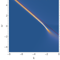
(a) $m=0.75$

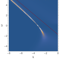
(b) $m=0.95$

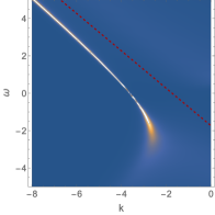
(c) $m=0.999$

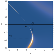
(d) $m=1.2$

Figure 1: $m$-Evolution of the spectral density for $p=1/2$. We have k-gap only if $m>m_{c}\simeq 0.96$. (d) also shows the definition of ($k_{C},\omega_{C}$) as the tip position.

Now we move to the case $p>1$. Here it is most interesting to see the evolutions across the $m=1/2$, which is drawn in Figure 2. The key result is that k-gap appears whenever $m$ is bigger than 1/2. That is, for large enough Pauli term, unitarity violation always gives instability. This is the kind of the phenomena expected in the regime where the unitarity bound is violated and indeed it happens.

(a) $m=0.3$

(b) $m=0.4$

(c) $m=0.6$

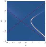
(d) $m=0.7$

Figure 2: $m$-Evolution across the $m=1/2$ with $p=2$ fixed. k-gap appears for any $m>1/2$. Red dotted line denotes IR light cone. When $m=1/2$, spectral density coincides with IR light cone

Figure 3 collectively describes the evolution of the dispersion curve as we change the $m$ for $p=5$. Starting from $m=0$ which belongs to the gapped phase, it arrives at the free fermion like phase at $m=1/2$, and finally it runs into the k-gapped state when $m>1/2$. This is very analogous to of the phenomenon that appears in the recent workBaggioli:2018vfc ; Baggioli:2018nnp describing a transition in transverse phonon dispersion from solid to liquids. In drawing the Figure 3, we used the method locus of ${\rm Re}G^{-1}=0$, which will be described in appendix.

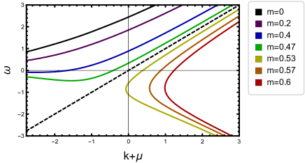
Figure 3: Mass evolution of spectral density at $p=5$. Dashed line denotes free fermion dispersion, $\omega=k+\mu$.

3.2 Fate of the vacuum and the Charge Density Wave

To see the nature of the instability, we calculated the density dependence of the position of $k_{C}$ and found that there is a linear relation between them. See Figure 4(a). The strong correlation between the charge density and the wave vector at the instability indicates that the instability is associated to the charge density wave.

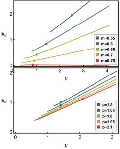
(a) Density dependece of $k_{c}$

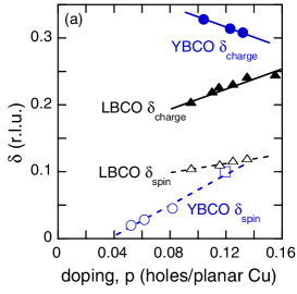
(b) CDW vector vs doping

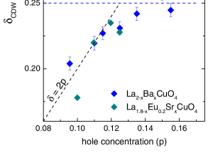
(c) bending data

Figure 4: (a) Linear dependence of $k_{C}$ in $\mu$, suggesting that the instability is toward the charge density wave (CDW). We choose $p=1.8$ (upper panel) and $m=0.6$ (lower panel). The dots are the location of $k_{C}^{*}$. (b,c) The doping dependence of CDW vector $\bf\delta$. The figure (b) is reproduced from blackburn2013x and figure (c) is from blanco2014resonant .

The Figure 4(b)(c) is reproduced from blackburn2013x , where linear dependence of the charge density wave vector $\bf\delta$ in the doping which is comparable to our charge density $Q$, which is related to $\mu$ by $Q=\mu r_{0}$ and $r_{0}=(2\pi T+\sqrt{(2\pi T)^{2}+3\mu^{2}})/3$. Therefore for $\mu/T<<1$, the density and the chemical potential is also linear each other. Since the doping parameter should be interpreted as the charge density the linear dependence of wave vector in the doping parameter is consistent with our theory at least for the low doping.

For higher doping or charge density, $r_{0}\sim\mu$ so that $Q\sim\mu^{2}$ as expected from the dimensional analysis or the non-interacting Fermi gas theory. Therefore our theory shows $k_{C}\sim\sqrt{Q}$. Figure 4(c) shows the a bit more recent data which shows bending of the data, which is consistent with our theory although the authors of the paper blanco2014resonant tried to fit with linear plot without success. Although we do not aim to detailed match of our theory with the data, it is encouraging to see that the general trend of data vs theory is consistent. This is our main result.

Notice that the linearity of doping and the wave vector is not a character of weakly interacting system but that of a strongly interacting one. Also if we consider the charge in our theory as the ’conserved’ spin, we would get the spin density wave instead of the CDW.

What would be the physical mechanism to create such unitarity bound violation? In a theory with Fermi surface(FS), CDW is associated with the nestingRice:1975aa ; WHANGBO_1991 , a phenomena associated with a shape of FS where a single vector $k_{Q}$ connects large parallel regions of a FS. In perturbation theory, it can lead to divergent scattering amplitude through $\int dk/(E_{k}-E_{k+q})\cdots$ for $q=k_{Q}$ and $k\in$ $\{$Nesting region$\}$. In the situation where Pauli principle is relaxed due to strong interaction so that the degrees of freedom relatively deep inside the Fermi sea can be excited, the nesting mechanism can work even in the absence of the Fermi surface. In more physical terms, such divergence can be rephrased as the appearance of large degrees of freedom that can interact effectively at a special momentum transfer $q=k_{Q}$, which is very similar to the unitarity violation in our theory. Therefore it is natural to identify the tip of the k-gap as the density wave vector: $k_{C}=k_{Q}$.

3.3 A measure of instability

When the tip is located at the Fermi level, the instability is most vivid because the Fermi velocity diverges there. The degree of super-luminosity, $v_{F}-1$, can be used as a measure of the instability:

$$D_{ins}={v_{F}-1}.$$ (15)

When $D_{ins}=\infty$, the instability can happen spontaneously, while the system is barely unstable if $D_{ins}=0$. Figure 5(a) plot the trajectory of $D_{ins}=\infty$ where spontaneous $k$-gap generation appear in parameter space of $(p,m,k_{C}^{*})$. Here $k_{C}^{*}$ is the value of $k$ at the tip of the k-gap and we interpret it as the wave vector of charge density wave. For any desired criterion $D_{0}$, $D_{ins}>D_{0}$ define a tubular neighborhood along the trajectory where charge density wave is formed with easiness $D_{0}$.

Figure 5(b) shows $m$-trajectory of the tip $(k_{C},\omega_{C})$ in the momentum space for a few different values of $p$. In the figure, the arrow indicates the direction of increasing $m$. There are three different classes of trajectories according to the range of $p$.

1. For $p<1.3$, $\omega_{C}$ is always negative and hence there is no spontaneous $k$-gap generation.

2. For $1.3\leq p\leq 2.3$, $\omega_{C}>0$ if $m\simeq 1/2$. The tip moves down as $m$ increases and passes Fermi level where the Fermi velocity diverges. If we increase mass further, then the tip position moves up and down so that the tip position pass $\omega=0$ line three times in total.

3. For $p>2.3$, the position of tip starts from $\omega>0$ region and pass $\omega=0$ line for $m\sim 1.5$.

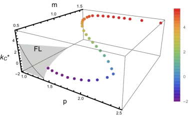
(a) Spontaneous CDW instability

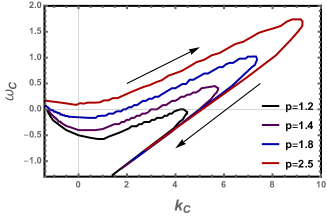
(b) $m$-trajectory of the tip position

Figure 5: (a) Trajectory of Spontaneous CDW: $D_{ins}=\infty$ along the dotted line. (b) Trajectory of the tip ($k_{C},\omega_{C}$) drawn as a parametric plot as $m$ move: Arrow indicates direction of increasing mass.

Notice that in the regime $p<1,m<m_{c}$ there is a region where k-gap or ghost spectrum does not appear in spite of the unitarity violation. See the shaded region of 5(b). This may be the fermionic analogue of the phenomena found in ref. Andrade:2011dg where it is shown for the scalar that there is a ghost free region in spite of the violation of the stability bound.

4 Discussion

In this paper, we calculated the spectral density of probe fermion with Pauli term above the unitarity limit and found a characteristic k-gap for most parameter regime which indicate that the system has instability. To show that the toward the density wave, we calculated the density dependence of the tip of the k-gap. It turns out that it agree with the doping dependence the wave number for physical system with CDW instability. This suggest that we can look for the spectrum and read off the wave number of the CDW by looking at the position of the tip of the k-gap.

To discuss the physical mechanism for the unitarity violation causing the k-gap and CDW, we point out that there is a similarity of unitarity bound violation and the nesting phenomena: in both cases one can observe the appearance of large degrees of freedom that can interact very effectively at a special momentum deliverance. We emphasize that our method did not introduce explicit inhomogeneity.

We speculate that out of all possible fermion coupling $B_{{\mu\nu\cdots}}{\bar{\psi}}\Gamma^{{\mu\nu\cdots}}\psi$ with $B_{{\mu\nu\cdots}}$ being a linear function of $A_{t}$ and its derivatives, Pauli term is the only one that can generate the gap.

Note added After this work is uploaded to archive, we were informed that similar related idea were discussed in recent papers Amoretti_2018 ; Amoretti_2018_2 ; Musso:2018wbv , where low energy scaling dimension was gravitationally calculated as a function of momentum and instability was identified as breaking its reality.

Appendix

Appendix A Tracer of spectral function peak

We used locus of $C=0$ method in drawing Figure 3. Here we want to describe it. If we write the retarded Green’s function as $G_{R}^{-1}={C-iD}$ with real $C$ and $D$,

$$A=ImG_{R}={D}/{(C^{2}+D^{2})}.$$ (16)

For finite $D$, the spectral density has its maximum at $C=0$. Therefore, one can easily check peak of spectral density by looking zero of $C$. It depends on the value of $D$ also. When $C=0$, the spectral density becomes $A=1/D$, hence it is suppressed when $D$ is large. To test how useful this idea is, we calculate the zero of $C$ for $m<1/2$ and compare with the spectral function. The comparison to the spectral density and the zero of $C$ are drawn in Figure 6, from which we can see that the two are well matched, although they do not exactly overlap.

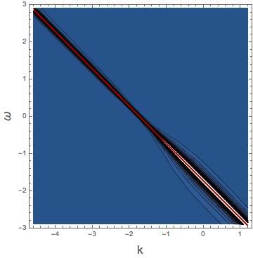
(a) $m=0.5$, $p=0$

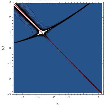
(b) $m=0.5$, $p=5$

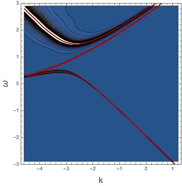
(c) $m=0.47$, $p=5$

Figure 6: The zero of $C$ (red line) vs. the peak of spectral function. We use unsymmetrized $G_{2}$. (a) Here zero of $C$ overlap with the pole of the Green function. (b) The new branch of dispersion curve created by the interaction and it is not followed by the zero of $C$. (c) Decreasing of $m$ from 1/2 deforms the original dispersion curve is and the zero of $C$ follows it, of but not the new branch.

Features of Figure 6 are described below.

1. Figure (a): At $p=0$, the peak of spectral function is same as zero of $C$.

2. Figure (b): The interaction generate new band along the maximum of $D$, Out of $C=0$ line, $C>>D$ so that $A\sim D/C^{2}$.

3. Figure (c): For $m$ off $1/2$, the original linear dispersion curve deform and the zero of $C$ follow it. peaks of both band are overlapped to the zero of $C$. But there is another branch of zero of C, which is the middle band in the figure, which is not realized as the peak of the spectral function. Along this band, $D$ has maximum value and the peak is suppressed since $A\sim 1/D$.

In Figure 7, we give some other comparison to test the method. We compared the spectral density and the locus of $C=0$ for $m$-Evolution with $p=2$ fixed. As one can see, almost precise agreement is obtained between the two. Summarizing, the real part of $G^{-1}$, contains the essential information for the peak of spectral density.

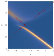
(a) $m=0.3$

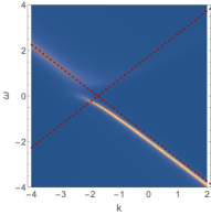
(b) $m=0.4$

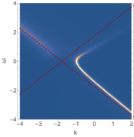
(c) $m=0.6$

(d) $m=0.7$

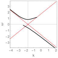
(e) $m=0.3$

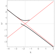
(f) $m=0.4$

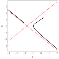
(g) $m=0.6$

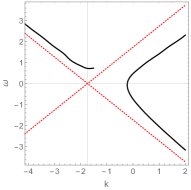
(h) $m=0.7$

Figure 7: Camparing the spectral density and locus of $C=0$ for $m$-Evolution across the $m=1/2$ with $p=2$ fixed. Precise agreement is obtained.

Appendix B Phase diagram

Once we know that the new vacuum has charge density wave, can we figure out more details about the phases of the system after CDW transition happen?

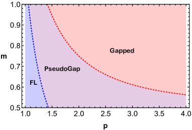
(a) Phase diagram

Figure 8: Phase diagram for $0.5<m<1.0$ with the unstable k-gapped band ignored. FL means gapless Fermi liquid like phase.

Since we know that the instability will be resolved by developing a gap, our recipe of the system for the new phase is simply neglecting the k-gapped branch of the spectral density. Here we speculate that we can classify the phases of the system with only other features in the spectral function. The phase diagram with such scheme is drawn in Figure 8 for $0.5<m<1.0$. Dashed line implies that these ‘phases’ are smoothly interpolated. The truth fate of the system should be calculated with explicit introduction of the non-homogeneity which will be much heavier this this work.

- (1) M. H. Whangbo, E. Canadell, P. Foury and J. P. Pouget, Hidden fermi surface nesting and charge density wave instability in low-dimensional metals, Science 252 (Apr, 1991) 96–98.
- (2) Y. Ling, C. Niu, J. Wu, Z. Xian and H.-b. Zhang, Metal-insulator Transition by Holographic Charge Density Waves, Phys. Rev. Lett. 113 (2014) 091602, [1404.0777].
- (3) A. Amoretti, D. Aren, B. Goutraux and D. Musso, Effective holographic theory of charge density waves, Phys. Rev. D97 (2018) 086017, [1711.06610].
- (4) T. Andrade, A. Krikun, K. Schalm and J. Zaanen, Doping the holographic Mott insulator, 1710.05791.
- (5) M. Edalati, R. G. Leigh, K. W. Lo and P. W. Phillips, Dynamical Gap and Cuprate-like Physics from Holography, Phys. Rev. D83 (2011) 046012, [1012.3751].
- (6) M. Edalati, R. G. Leigh and P. W. Phillips, Dynamically Generated Mott Gap from Holography, Phys. Rev. Lett. 106 (2011) 091602, [1010.3238].
- (7) H. Liu, J. McGreevy and D. Vegh, Non-Fermi liquids from holography, Phys. Rev. D83 (2011) 065029, [0903.2477].
- (8) U. Gursoy, E. Plauschinn, H. Stoof and S. Vandoren, Holography and ARPES Sum-Rules, JHEP 05 (2012) 018, [1112.5074].
- (9) Y. Seo, G. Song, Y.-H. Qi and S.-J. Sin, Mott transition with Holographic Spectral function, 1803.01864.
- (10) S.-S. Lee, A Non-Fermi Liquid from a Charged Black Hole: A Critical Fermi Ball, Phys. Rev. D79 (2009) 086006, [0809.3402].
- (11) T. Faulkner, H. Liu, J. McGreevy and D. Vegh, Emergent quantum criticality, Fermi surfaces, and AdS(2), Phys. Rev. D83 (2011) 125002, [0907.2694].
- (12) T. Faulkner, N. Iqbal, H. Liu, J. McGreevy and D. Vegh, Holographic non-Fermi liquid fixed points, Phil. Trans. Roy. Soc. A 369 (2011) 1640, [1101.0597].
- (13) T. Faulkner, N. Iqbal, H. Liu, J. McGreevy and D. Vegh, Charge transport by holographic Fermi surfaces, Phys. Rev. D88 (2013) 045016, [1306.6396].
- (14) J. Zaanen, Y.-W. Sun, Y. Liu and K. Schalm, Holographic Duality in Condensed Matter Physics. Cambridge Univ. Press, 2015.
- (15) S. A. Hartnoll, A. Lucas and S. Sachdev, Holographic quantum matter, 1612.07324.
- (16) M. Cubrovic, J. Zaanen and K. Schalm, String Theory, Quantum Phase Transitions and the Emergent Fermi-Liquid, Science 325 (2009) 439–444, [0904.1993].
- (17) M. Cubrovic, J. Zaanen and K. Schalm, Constructing the AdS Dual of a Fermi Liquid: AdS Black Holes with Dirac Hair, JHEP 10 (2011) 017, [1012.5681].
- (18) M. Baggioli and K. Trachenko, Solidity of liquids: How Holography knows it, 1807.10530.
- (19) M. Baggioli and K. Trachenko, Maxwell interpolation and close similarities between liquids and holographic models, 1808.05391.
- (20) E. Blackburn, J. Chang, M. Hücker, A. Holmes, N. B. Christensen, R. Liang et al., X-ray diffraction observations of a charge-density-wave order in superconducting ortho-ii yba 2 cu 3 o 6.54 single crystals in zero magnetic field, Physical review letters 110 (2013) 137004.
- (21) S. Blanco-Canosa, A. Frano, E. Schierle, J. Porras, T. Loew, M. Minola et al., Resonant x-ray scattering study of charge-density wave correlations in yba 2 cu 3 o 6+ x, Physical Review B 90 (2014) 054513.
- (22) T. M. Rice, New mechanism for a charge-density-wave instability, Physical Review Letters 35 (1975) 120–123.
- (23) T. Andrade and D. Marolf, AdS/CFT beyond the unitarity bound, JHEP 01 (2012) 049, [1105.6337].
- (24) A. Amoretti, D. Areán, B. Goutéraux and D. Musso, Effective holographic theory of charge density waves, Physical Review D 97 (Apr, 2018) .
- (25) A. Amoretti, D. Areán, B. Goutéraux and D. Musso, dc resistivity of quantum critical, charge density wave states from gauge-gravity duality, Physical Review Letters 120 (Apr, 2018) .
- (26) D. Musso, Simplest phonons and pseudo-phonons in field theory, 1810.01799.