An augmented Lagrangian preconditioner for the 3D stationary incompressible Navier–Stokes equations at high Reynolds number

Abstract

In Benzi & Olshanskii (SIAM J. Sci. Comput., 28(6) (2006)) a preconditioner of augmented Lagrangian type was presented for the two-dimensional stationary incompressible Navier–Stokes equations that exhibits convergence almost independent of Reynolds number. The algorithm relies on a highly specialized multigrid method involving a custom prolongation operator and for robustness requires the use of piecewise constant finite elements for the pressure. However, the prolongation operator and velocity element used do not directly extend to three dimensions: the local solves necessary in the prolongation operator do not satisfy the inf-sup condition. In this work we generalize the preconditioner to three dimensions, proposing alternative finite elements for the velocity and prolongation operators for which the preconditioner works robustly. The solver is effective at high Reynolds number: on a three-dimensional lid-driven cavity problem with approximately one billion degrees of freedom, the average number of Krylov iterations per Newton step varies from 4.5 at $\mathrm{Re}=10$ to 3 at $\mathrm{Re}=1000$ and 5 at $\mathrm{Re}=5000$.

65N55, 65F08, 65N30

1 Introduction

We consider the stationary incompressible Newtonian Navier–Stokes equations: given a bounded Lipschitz domain $\Omega\subset\mathbb{R}^{d}$, $d\in\{2,3\}$, find $(u,p)\in{H}^{1}(\Omega;\mathbb{R}^{d})\times Q$ such that

(1a) $$-\nabla\cdot 2\nu\varepsilon(u)+(u\cdot\nabla)u+\nabla p =f\quad \text{ in }\Omega,$$

(1b) $$\nabla\cdot u =0\quad \text{ in }\Omega,$$

(1c) $$u =g\quad \text{ on }\Gamma_{D},$$

(1d) $$2\nu\varepsilon(u)\cdot n =pn\quad \text{ on }\Gamma_{N},$$

where $\varepsilon(u)=\frac{1}{2}(\nabla u+\nabla u^{T})$, $\nu>0$ is the kinematic viscosity, $f\in{L}^{2}(\Omega;\mathbb{R}^{d})$, $n$ is the outward-facing unit normal to $\partial\Omega$, $\Gamma_{D}$ and $\Gamma_{N}$ are disjoint with $\Gamma_{D}\cup\Gamma_{N}=\partial\Omega$, and $g\in H^{1/2}(\Gamma_{D};\mathbb{R}^{d})$. If $|\Gamma_{N}|>0$, then a suitable trial space for the pressure is $Q:={L}^{2}(\Omega)$; if $|\Gamma_{N}|=0$, then the pressure is only defined up to an additive constant and $Q:=L^{2}_{0}(\Omega)$ is used instead. The Reynolds number, defined as $\mathrm{Re}=\frac{UL}{\nu}$ where $U$ is the characteristic velocity and $L$ is the characteristic length scale of the flow, is an important dimensionless number governing the nature of the flow. The Navier–Stokes equations are of enormous practical importance in science and industry, but are very difficult to solve, especially for large Reynolds number. The importance of these equations has motivated a great deal of research on algorithms for their solution; for a general overview of the field, see the textbooks of Turek [77], Elman, Silvester & Wathen [30], or Brandt [16].

After Newton linearization and a suitable spatial discretization of (1), nonsymmetric linear systems of saddle point type must be solved:

(2) $$\begin{pmatrix}A&B^{T}\\ B&0\end{pmatrix}\begin{pmatrix}\delta u\\ \delta p\end{pmatrix}=\begin{pmatrix}b\\ c\end{pmatrix},$$

where $A$ is the discrete linearized momentum operator, $B^{T}$ is the discrete gradient operator, $B$ is the discrete divergence operator, and $\delta u$ and $\delta p$ are the updates to the coefficients for velocity and pressure respectively. One strategy to solve these systems is to employ a monolithic multigrid iteration on the entire system with a suitable coupled relaxation method, such as the algorithms of Vanka [79] or Braess & Sarazin [15]. Vanka iteration works well for moderate Reynolds numbers [77], but the iteration counts have been observed to increase significantly once the Reynolds number becomes large [7].

An alternative approach to solving (2) is to build preconditioners based on block factorizations [58, 43, 6, 30, 80]. This strategy can be grounded in an insightful functional analytic framework that guides the development of solvers whose convergence is independent of parameter values and mesh size $h$, at least in the case where (2) is symmetric [56]. Block Gaussian elimination reduces the problem of solving the coupled linear system to that of solving smaller separate linear systems involving the matrix $A$ and the Schur complement $S=-BA^{-1}B^{T}$. If a fast solver is available for $A$, the main difficulty is solving linear systems involving $S$, as this matrix is generally dense and cannot be stored explicitly for large problems. Tractable approximations $\tilde{S}^{-1}$ to $S^{-1}$ must be devised on a PDE-specific basis.

For the Stokes equations, the Schur complement is spectrally equivalent to the viscosity-weighted pressure mass matrix [74]. For the Navier–Stokes equations this choice yields mesh-independent convergence and is effective for very small Reynolds numbers, but the convergence deteriorates badly with Reynolds number [27, 30]. The pressure convection-diffusion (PCD) approach [46] constructs an auxiliary convection-diffusion operator on the pressure space, and hypothesizes that a certain commutator is small. This yields an approximation to the Schur complement inverse that involves the inverse of the Laplacian on the pressure space, the application of the auxiliary convection-diffusion operator, and the inverse of the pressure mass matrix. The least-squares commutator (LSC) approach [26] is based on a similar idea, but derives the commutator algebraically. Both of these approaches perform well for moderate Reynolds numbers. Numerical experiments comparing the performance of our approach to these algorithms are provided in section 5.

In 2006, Benzi & Olshanskii proposed an augmented Lagrangian approach for controlling the Schur complement of (2) [60, 7, 59, 8, 31, 51]. The idea, referred to as grad-div stabilization, is to introduce an additional term in the equations that does not change the continuous solution, but does modify the Schur complement. The continuous form of the stabilization replaces (1a) with

(3) $$-\nabla\cdot 2\nu\varepsilon(u)+(u\cdot\nabla)u+\nabla p-\gamma\nabla\nabla\cdot u =f\quad \text{ in }\Omega,$$

for $\gamma>0$. As $\nabla\cdot u=0$, the solutions of (3) and (1a) are the same. The discrete variant of this approach replaces (2) with

(4) $$\begin{pmatrix}A+\gamma B^{T}M_{p}^{-1}B&B^{T}\\ B&0\end{pmatrix}\begin{pmatrix}\delta u\\ \delta p\end{pmatrix}=\begin{pmatrix}b+\gamma B^{T}M_{p}^{-1}c\\ c\end{pmatrix},$$

where $M_{p}$ is the pressure mass matrix. This modified system has the same discrete solutions as (2), as $B\delta u=0$. With either variant, for $\gamma$ not too small, the Schur complement inverse is well approximated by

(5) $$S^{-1}\approx-(\nu+\gamma)M_{p}^{-1},$$

where $M_{p}$ is the pressure mass matrix. This approximation improves as $\gamma$ increases (section 3). In either case, we denote the discretized augmented momentum block as $A_{\gamma}$.

Remark .

The continuous form of the grad-div stabilization has some further appealing characteristics. For example, it significantly improves the pressure-robustness of discretizations where the incompressibility constraint is not enforced pointwise [60, 40, 44]. It also arises in other contexts in the numerical analysis of (1). For example, Boffi & Lovadina [13] showed that the addition of the term $h^{-1/2}(\nabla\cdot u,\nabla\cdot v)_{{L}^{2}(\Omega)}$ to the weak form of the $[\mathbb{P}_{2}]^{2}\mathrm{-}\mathbb{P}_{0}$ discretization of (1) improves its convergence order. It also arises in the iterated penalty [76, 17] and artificial compressibility [22] methods for the Stokes and Navier–Stokes equations.

The tradeoff with either variant of this approach is that developing fast solvers for $A_{\gamma}$ becomes significantly more difficult. The divergence operator has a large kernel (the range of the curl operator) and hence standard multigrid relaxation methods are ineffective.

A key insight of Benzi & Olshanskii was that a specialized multigrid algorithm could be built for $A_{\gamma}$ [7, 59] by applying the seminal work of Schöberl [68]. The algorithm combines four ingredients, each of which is crucial to the effectiveness of the method: (i) the discrete variant of the grad-div stabilization; (ii) streamline-upwind Petrov-Galerkin (SUPG) stabilization of the advective term; (iii) a multigrid relaxation that effectively treats errors in the kernel of the discrete divergence term; (iv) a specialized prolongation operator whose continuity constant is independent of $\gamma$ and $\nu$. This scheme exhibits outer iteration counts that grow only very slowly with Reynolds number [7]. However, it is described as difficult to implement [37, 9], and so most of the works that use grad-div stabilization and the Schur complement approximation (5) employ either matrix factorization as the inner solver [24, 78, 14, 38, 40] or a block-triangular approximation to $A_{\gamma}$ [9, 37, 8, 39]. This block-triangular approximation decouples linear systems involving $A_{\gamma}$ into $d$ scalar anisotropic advection–diffusion problems, which may be solved with algebraic multigrid techniques. However, this simplicity comes at a price; the scheme is much more sensitive to the choice of $\gamma$, and its convergence deteriorates somewhat as the Reynolds number increases [9].

The main contribution of this paper is the extension of the robust multigrid scheme for the inner velocity problem arising in the augmented Lagrangian preconditioner to three dimensions. The previous work of Benzi & Olshanskii only considered the case $d=2$. While the same general strategy applies in three dimensions, the extension is nontrivial: if the finite elements used in [68, 7] are applied in three dimensions, the prolongation operator involves the solution of ill-posed local problems. We propose appropriate finite element discretizations and matching prolongation operators that exhibit Reynolds-robust iteration counts in three dimensions.

A second contribution is the release of an open-source parallel implementation of the solver in two and three dimensions, built on Firedrake [66] and PETSc [5]. This has required substantial modifications to Firedrake, PETSc, UFL [1] and TSFC [42], as well as minor developments in FIAT [47]. The solver heavily relies on and extends the solver infrastructure developed in [48], enabling easy composition and nesting of preconditioners in PETSc and Firedrake. To express the local solves involved in the relaxation and prolongation operator, we have developed a new preconditioner in PETSc that allows for the simple expression of general additive subspace correction methods. For example, the same code that does patchwise relaxation can be used to formulate line smoothers, plane smoothers, or Vanka iteration, and we expect that it will be of substantial interest for other applications as well.

The remainder of the paper is laid out as follows. The discretization and the grad-div stabilization are described in section 2. The augmented Lagrangian approach is explained in section 3. The multigrid cycle for the augmented momentum block is described in section 4. Numerical experiments analyzing its performance and comparing it to PCD and LSC are reported in section 5. Finally, conclusions and prospects for future improvements are given in section 6.

2 Formulation and discretization

For boundary data $g\in H^{1/2}(\Gamma_{D})$, let

(6) $$V_{g}=\{v\in H^{1}(\Omega;\mathbb{R}^{d}):\left.v\right|_{\Gamma_{D}}=g\}.$$

The initial weak form of (1) is: find $(u,p)\in V_{g}\times Q$ such that

(7) $$\int_{\Omega}2\nu\varepsilon(u):\nabla v\ \mathrm{d}x+\int_{\Omega}(u\cdot\nabla)u\cdot v\ \mathrm{d}x-\int_{\Omega}p\nabla\cdot v\ \mathrm{d}x-\int_{\Omega}q\nabla\cdot u\ \mathrm{d}x=\int_{\Omega}f\cdot v\ \mathrm{d}x,$$

for all $(v,q)\in V_{0}\times Q$. This will be extended before discretization in two ways. The first is a consistent SUPG stabilization; it is well known that straightforward Galerkin discretizations of advection-dominated problems are oscillatory [19, 77, 64, 30]. In addition, it is widely observed that mesh-dependent SUPG stabilization is highly advantageous for multigrid smoothers on advection-dominated problems [65, 77]. The strong form of the momentum residual is given by

(8) $$\mathcal{L}(u,p)=-\nabla\cdot 2\nu\varepsilon(u)+(u\cdot\nabla)u+\nabla p-f$$

and the following term is added to the weak form:

(9) $$\int_{\Omega}\delta(u)\mathcal{L}(u,p)\cdot\big{(}(u\cdot\nabla)v\big{)}\ \mathrm{d}x.$$

Here $\delta(u)$ is a weighting function that should be small in regions where the flow is well-resolved and large where stabilization is necessary. The particular form employed in this work is

(10) $$\delta(u)=\delta_{d}\left(\frac{4\|u\|^{2}}{h^{2}}+\frac{144\nu^{2}}{h^{4}}\right)^{-1/2},$$

with $\delta_{d}=1$ in two dimensions and $\delta_{d}=1/20$ in three dimensions. To the best of our knowledge this form was first suggested in [72, eq. (3.58)]. It is important to take account of the dependence of $\delta$ on the (unknown) solution $u$ when taking the derivatives required by Newton’s method; in this work, these derivatives are calculated automatically and symbolically by the Unified Form Language [1].

The second modification is the augmented Lagrangian term described above in (3) and (4). If the continuous variant is employed, the term

(11) $$\gamma\int_{\Omega}\nabla\cdot u\,\nabla\cdot v\ \mathrm{d}x$$

is added to the weak form, while if the discrete variant is employed, the term

(12) $$\gamma\int_{\Omega}\big{(}\mathrm{P}_{Q_{h}}\nabla\cdot u\big{)}\nabla\cdot v\ \mathrm{d}x$$

is added instead, where $\mathrm{P}_{Q_{h}}:L^{2}(\Omega)\to Q_{h}$ is the projection operator onto the discrete pressure space $Q_{h}$. The continuous grad-div stabilization changes the discrete solution computed if the discrete velocity $u_{h}$ does not satisfy $\nabla\cdot u_{h}=0$ pointwise, whereas the discrete variant does not. The effect of the continuous approach is to penalize $\|\nabla\cdot u_{h}\|_{L^{2}(\Omega)}$ and thereby improve the discrete enforcement of the incompressibility constraint [60, 40, 44]. Nevertheless, in this work we use the discrete variant (12). The reason for this is that the kernel of $\mathrm{P}_{Q_{h}}\mathrm{div}$ is much more straightforward to characterize than the kernel of $\mathrm{div}$ if $Q_{h}$ is chosen to be the space of piecewise constants:

(13) $$Q_{h}(\mathcal{M})=\{q\in L^{2}(\Omega):\left.q\right|_{K}\in\mathbb{P}_{0}(K)\ \forall K\ \in\mathcal{M}\},$$

where $\mathcal{M}$ is a simplicial mesh of the domain $\Omega$. By the divergence theorem, $u_{h}\in\mathrm{ker}(\mathrm{P}_{Q_{h}}\mathrm{div})$ if and only if for any $K\in\mathcal{M}$, $u_{h}$ satisfies

(14) $$\int_{\partial K}\!u_{h}\cdot n\ \mathrm{d}s=0.$$

This characterization will be extremely useful for dealing with errors in the kernel in the multigrid relaxation, as it ensures that the kernel is spanned by basis functions with local support [18, §VI.8]. Note also that this choice of $Q_{h}$ removes the dependency of $\mathcal{L}$ on $p$ (as $\nabla p$ is zero on each element), thereby eliminating any extra contribution to the top-right block of the linearized system to be solved, thus preserving the symmetry between the top-right and bottom-left blocks of the matrix.

After these modifications, the final discrete weak form to be solved is: find $(u,p)\in\big{(}V_{h}\cap V_{g}\big{)}\times\big{(}Q_{h}\cap Q\big{)}$ such that

$$\ \int_{\Omega}2\nu\varepsilon(u):\nabla v\ \mathrm{d}x+\int_{\Omega}(u\cdot\nabla)u\cdot v\ \mathrm{d}x+\int_{\Omega}\delta(u)\mathcal{L}(u)\cdot\big{(}(u\cdot\nabla)v\big{)}\ \mathrm{d}x$$

(15) $$+\gamma\int_{\Omega}\big{(}\mathrm{P}_{Q_{h}}\nabla\cdot u\big{)}\nabla\cdot v\ \mathrm{d}x-\int_{\Omega}p\nabla\cdot v\ \mathrm{d}x-\int_{\Omega}q\nabla\cdot u\ \mathrm{d}x=\int_{\Omega}f\cdot v\ \mathrm{d}x,$$

for all $(v,q)\in\big{(}V_{h}\cap V_{0}\big{)}\times\big{(}Q_{h}\cap Q\big{)}$, with the choice of $V_{h}$ to be discussed below.

2.1 Choice of velocity space

We now turn our attention to choosing an appropriate space for the discrete velocities. Define the space $V_{h}(\mathcal{M})$ used for the velocity as

(16) $$V_{h}(\mathcal{M})=\{v\in H^{1}(\Omega):\left.v\right|_{K}\in\mathbb{P}_{v}(K)\ \forall\ K\in\mathcal{M}\},$$

for some choice of $\mathbb{P}_{v}(K)$. The first condition on $\mathbb{P}_{v}(K)$ is that $V_{h}$ must be inf-sup stable when combined with $Q_{h}$ for the pressure. Unfortunately, both in two and in three dimensions, the $[\mathbb{P}_{1}]^{d}-\mathbb{P}_{0}$ element combining piecewise linear functions for the velocity space together with piecewise constants for the pressure does not satisfy the inf-sup condition on general meshes. This means that the velocity space needs to be enriched, with the resulting element pairs (e.g. $[\mathbb{P}_{2}]^{2}\mathrm{-}\mathbb{P}_{0}$ and $[\mathbb{P}_{3}]^{3}\mathrm{-}\mathbb{P}_{0}$) exhibiting a suboptimal convergence rate.

In [7] the element pair $[\mathbb{P}_{1}\text{iso}\,\mathbb{P}_{2}]^{2}\mathrm{-}\mathbb{P}_{0}$ is used, which is obtained by considering a $[\mathbb{P}_{1}]^{2}$ element on a once refined mesh for the velocity. This element has the same number of degrees of freedom as $[\mathbb{P}_{2}]^{2}\mathrm{-}\mathbb{P}_{0}$. Neither $[\mathbb{P}_{2}]^{3}\mathrm{-}\mathbb{P}_{0}$ nor $[\mathbb{P}_{1}\text{iso}\,\mathbb{P}_{2}]^{3}\mathrm{-}\mathbb{P}_{0}$ are inf-sup stable on a single regularly refined tetrahedron, which as we shall see in section 4.2 is crucial for the effectiveness of the preconditioner. They are missing degrees of freedom on the facets of the tetrahedra which are necessary to stabilize the jump of the pressure field.

Increasing the degree of the velocity space to piecewise cubic polynomials, i.e. choosing the element pair $[\mathbb{P}_{3}]^{3}\mathrm{-}\mathbb{P}_{0}$, introduces additional degrees of freedom on the facets and results in a stable element pair. However, this element is extremely expensive while being suboptimal by two orders for the velocity. Alternatively, Bernardi & Raugel [10, 11] suggest enriching the piecewise linear velocity space with bubble functions on each facet. While it is only necessary to add a single bubble function for the normal component of the velocity on each facet, this adds significant complexity to the implementation as these functions are not affine equivalent; they require a Piola transform to preserve the normal orientation. This means that the basis functions associated with vertices and those associated with facets need to be pulled-back differently, complicating the implementation. For this reason we choose instead to enrich the space with facet bubbles for all three components of the velocity, obtaining the $[\mathbb{P}_{1}\oplus B^{F}_{3}]^{3}\mathrm{-}\mathbb{P}_{0}$ element. As can be seen in Figure 1, this results in an element with significantly fewer degrees of freedom than $[\mathbb{P}_{3}]^{3}\mathrm{-}\mathbb{P}_{0}$. We also show the $[\mathbb{P}_{2}\oplus B^{F}_{3}]^{3}$ element in Figure 1; we will demonstrate in Section 4.2 that these elements satisfy a particular property that is useful in the prolongation.

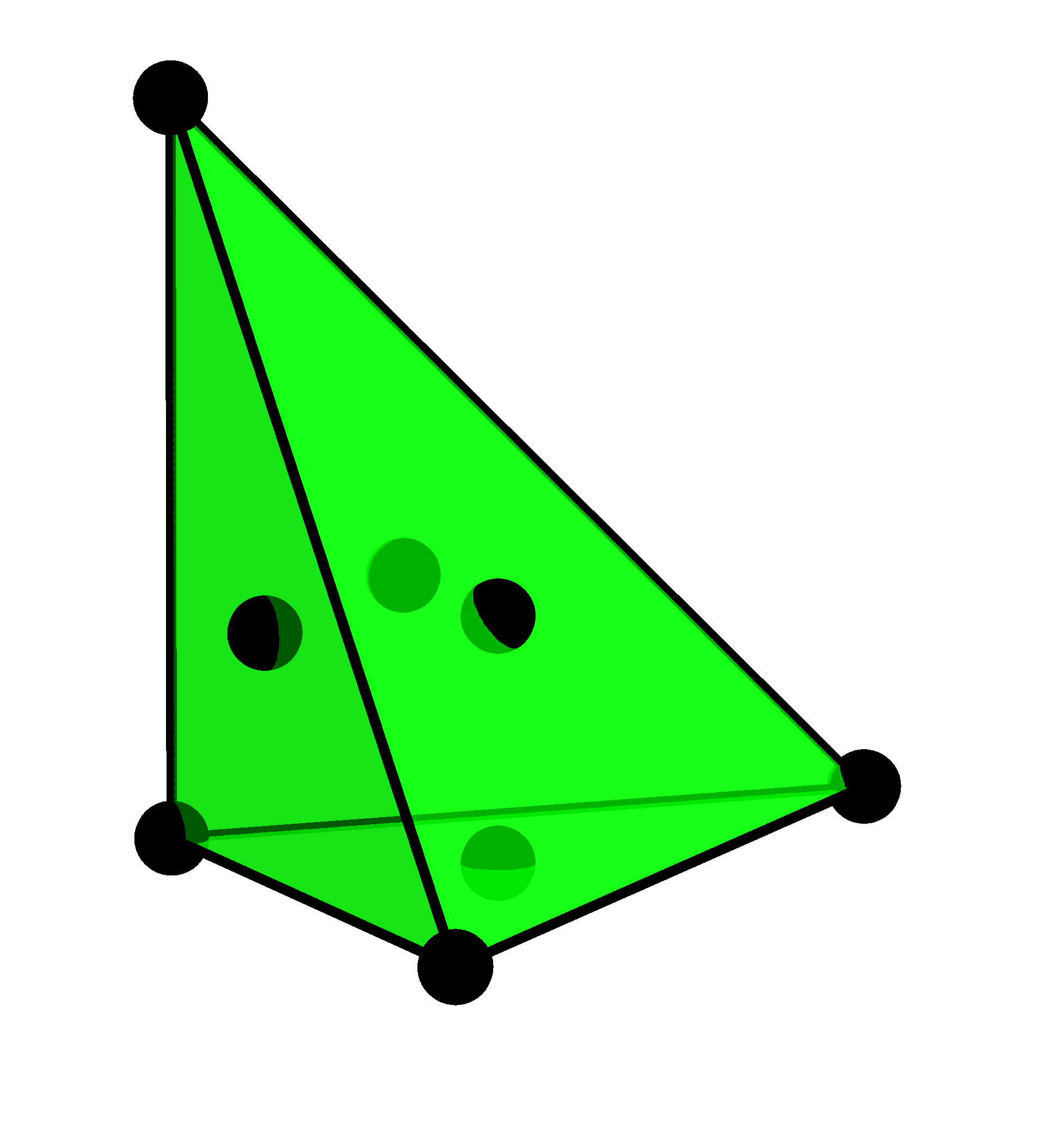
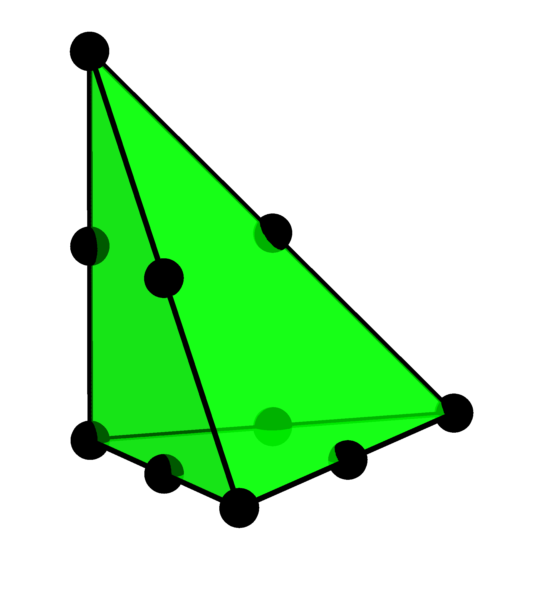
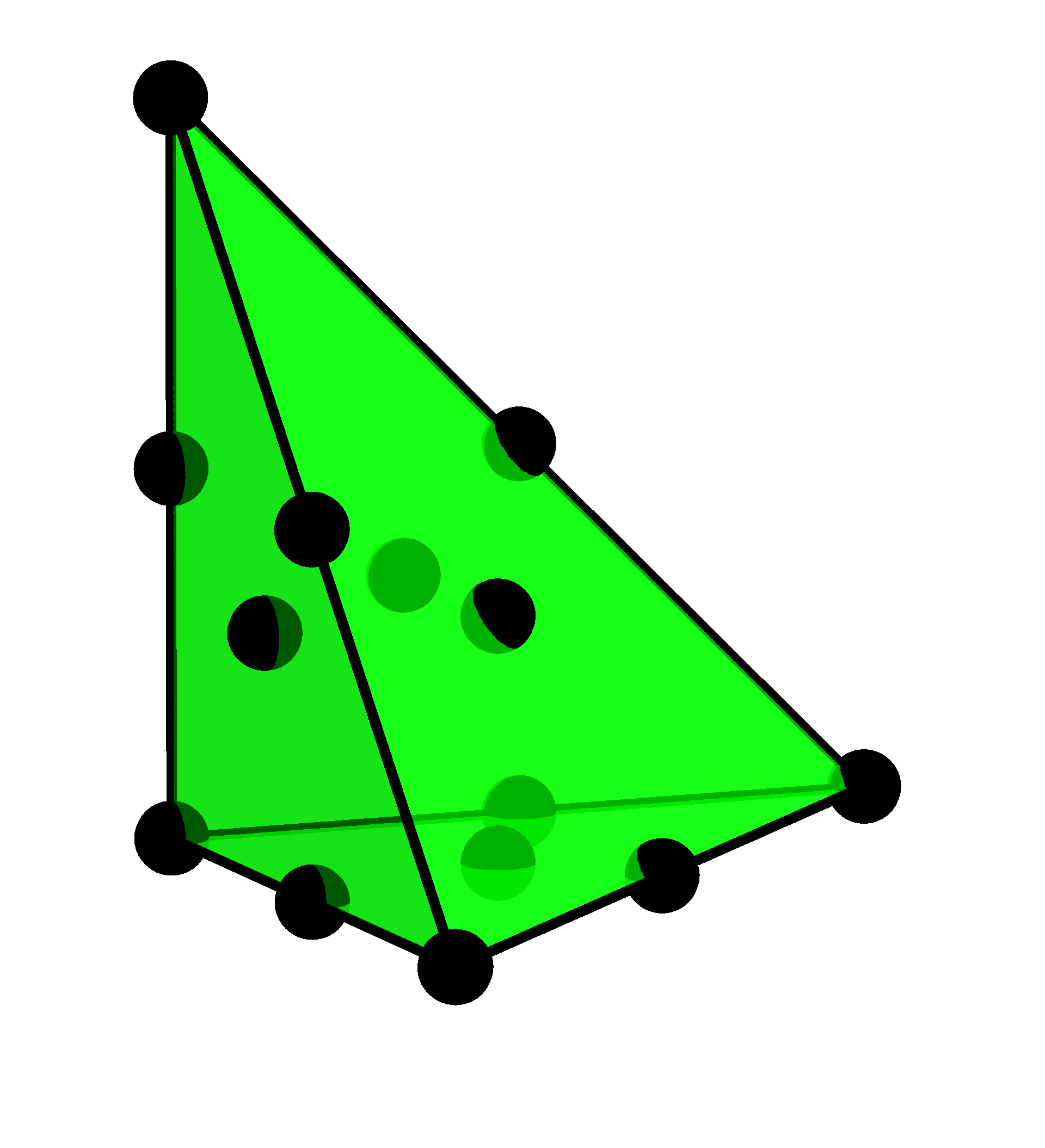
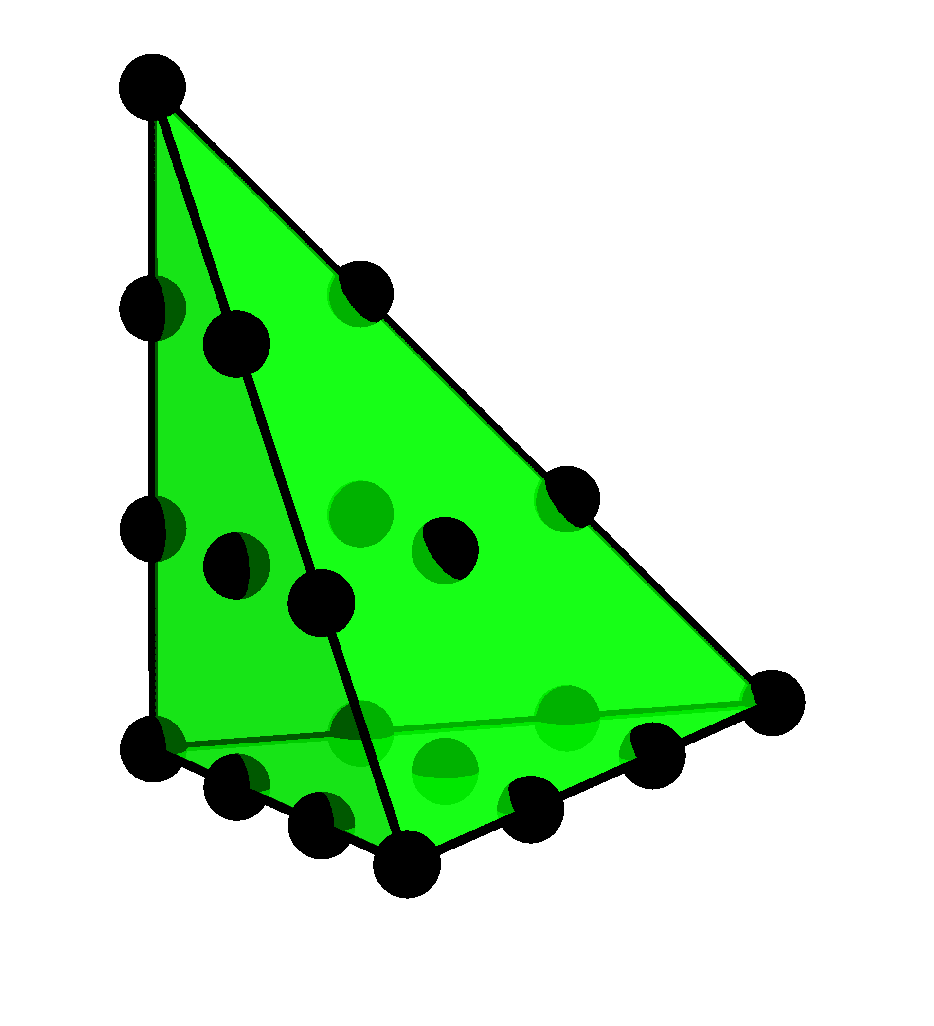
Figure 1: The $\mathbb{P}_{1}\oplus B^{F}_{3}$, $\mathbb{P}_{2}$, $\mathbb{P}_{2}\oplus B^{F}_{3}$ and $\mathbb{P}_{3}$ elements.

Remark .

Pressure elements other than $\mathbb{P}_{0}$ have been considered for the augmented Lagrangian preconditioner. Benzi & Olshanskii [7, Table 6.2] also present results for the $[\mathbb{P}_{1}\text{iso}\,\mathbb{P}_{2}]^{2}\mathrm{-}\mathbb{P}_{1}$ pair, where the pressure mass matrix solve in $\mathrm{P}_{Q_{h}}$ is approximated by the inverse of a diagonal matrix. However, for this element pairing the developed multigrid scheme is not independent of the ratio $\gamma/\nu$ and hence as $\nu$ decreases, $\gamma$ has to be decreased correspondingly. This in turn leads to worse control of the Schur complement and consequent growth in iteration counts.

Remark .

Effective smoothers for partial differential equations involving the continuous term $(\nabla\cdot u,\nabla\cdot v)_{L^{2}(\Omega)}$ have been proposed in other contexts [2, 41]; it should be possible to extend these approaches to the two- and three-dimensional advection-dominated case considered here, and thereby enable the use of finite elements with advantageous properties such as optimal convergence rates and exact enforcement of the incompressibility constraint.

3 The augmented Lagrangian method

The Schur complement of the matrix in (4) is given by

(17) $$S=-B(A+\gamma B^{T}M_{p}^{-1}B)^{-1}B^{T}.$$

From the Sherman–Morrison–Woodbury formula it follows (e.g. [4, Theorem 3.2]) that

(18) $$S^{-1}=-(BA^{-1}B^{T})^{-1}-\gamma M_{p}^{-1}.$$

From this we obtain immediately that

(19) $$\tilde{S}^{-1}=-(\nu+\gamma)M_{p}^{-1}$$

is a good approximation to $S^{-1}$ as $\gamma\to\infty$ for fixed mesh size and viscosity. To understand the quality of the approximation for finite $\gamma$ as $\nu$ or $h$ change, we need to consider how $\nu M_{p}^{-1}$ approximates $(BA^{-1}B^{T})^{-1}$.

It is well known that the eigenvalues of a matrix do not characterize the convergence of GMRES for a linear system [35]. Instead, it is necessary to bound the field-of-values of the preconditioned system [75, Theorem 3.2], [25, Corollary 6.2], [62, §1.3]. This analysis was performed by Benzi & Olshanskii [8] for both the ideal and the modified augmented Lagrangian preconditioner for the Oseen problem, using general results of Loghin & Wathen [55]. One of the key ingredients in this analysis is that the momentum operator is coercive with constant $\nu$. They use this to prove that the choice of $\gamma\sim\nu^{-1}$ results in an optimal preconditioner (assuming exact solves of the momentum block). However, it is well known [34, p. 300] that the momentum operator of the Newton linearization of (1) is only coercive for $\nu>\nu_{0}$ for some problem-dependent $\nu_{0}$. Fortin & Glowinski remark [31, p. 85] that this is typically a very restrictive condition: for $\nu>\nu_{0}$ the Stokes approximation itself is adequate. This proof strategy would therefore require significant extension to apply to the Newton linearization considered here.

In practice, Benzi & Olshanskii [7] observe that a constant choice of $\gamma$ yields mesh-independent and essentially Reynolds number independent results. As our multigrid solver for the momentum block is robust with respect to $\gamma$, we simply choose $\gamma$ large. In the experiments of section 5, we take the value $\gamma=10^{4}$, to match the largest Reynolds number considered.

4 Solving the augmented momentum block

The key challenge with the augmented Lagrangian strategy is the solution of the augmented momentum block $A_{\gamma}$. The grad-div term has a large nullspace, rendering standard relaxation methods (point-block Jacobi or Gauss–Seidel) ineffective as $\nu\to 0$. In this section we explain the specialized multigrid algorithm of Benzi & Olshanskii, along with the modifications required to extend the method to three dimensions. The multigrid method has two components: a $\nu$- and $\gamma$-robust relaxation method, and a kernel-preserving prolongation operator. In subsections 4.1 and 4.2 we first consider the augmented Stokes momentum operator without the linearized advection terms, to study in the simplest possible situation the difficulties arising with the grad-div term. We then comment on the case with advection in subsection 4.3.

To understand the properties required of the relaxation and prolongation, it suffices to consider a two-level scheme. We use the subscripts $h$ and $H$ to denote function spaces, bilinear forms, and meshes on the fine and coarse levels respectively.

4.1 Relaxation

The augmented Stokes momentum problem is of the form: find $u\in V_{h,0}:=V_{h}\cap V_{0}$ such that

(20) $$a_{h}(u,v)\coloneqq(2\nu\varepsilon(u),\nabla v)+\gamma(\mathrm{P}_{Q_{h}}\nabla\cdot u,\nabla\cdot v)=(f,v)$$

for all $v\in V_{h,0}$. The viscosity term is symmetric and positive definite; the discrete grad-div term is positive semidefinite. As $\nu\to 0$ or $\gamma\to\infty$ this system becomes nearly singular and standard relaxation methods such as Gauss–Seidel or Jacobi iterations perform poorly. The essential difficulty is in computing the component of the solution in the kernel

(21) $$\mathcal{N}_{h}:=\{u\in V_{h,0}:(\mathrm{P}_{Q_{h}}\nabla\cdot u,\nabla\cdot v)=0\ \forall\ v\in V_{h,0}\}$$

of the grad-div term. Schöberl [69, Theorem 4.1] and Lee et al. [52, Theorem 4.2] consider subspace correction methods for this class of problem. The key result of these works is that if a subspace decomposition

(22) $$V_{h,0}=\sum_{i}V_{i}$$

satisfies the kernel decomposition property

(23) $$\mathcal{N}_{h}=\sum_{i}\left(V_{i}\cap\mathcal{N}_{h}\right)$$

then the resulting subspace correction method (a block Gauss–Seidel or Jacobi iteration) is robust with respect to $\nu$ and $\gamma$. This is why characterizing the kernel of the grad-div term is crucial, and why the discrete variant is easier to solve: the kernel $\mathcal{N}_{h}$ is spanned by basis functions with local support around each vertex.

More specifically, for each vertex $v_{i}$ in the mesh $\mathcal{M}$, its star is the patch of elements sharing $v_{i}$:

(24) $$K_{i}\coloneqq\bigcup_{{K\in\mathcal{M}\,:\,v_{i}\in K}}K.$$

The subspace decomposition is then given by

(25) $$V_{i}\coloneqq\{\phi_{j}\in V_{h,0}:\mathrm{supp}(\phi_{j})\subset K_{i}\}.$$

We call the resulting patchwise block relaxation method a star iteration. Note that homogeneous Dirichlet conditions are imposed on the boundary of each star patch. This relaxation method has been employed for robust multigrid methods in $H(\mathrm{div})$ and $H(\mathrm{curl})$ [3].

For the reader’s convenience, we briefly summarize the argument of [69, Section 4.1.2] to see why this decomposition satisfies (23). Observe that a discretely divergence-free vector field $u_{h}\in\mathcal{N}_{h}$ can be suitably modified in the interior of each cell to become continuously divergence-free by solving a local Stokes problem. Denote this continuously divergence-free vector field by $\tilde{u}$ and recall that then $\tilde{u}=\nabla\times\phi$ for some vector field $\phi$. Choosing a partition of unity $\{\rho_{i}\}_{i}$ with $\sum_{i}\rho_{i}=1$ and $\mathrm{supp}(\rho_{i})\subset K_{i}$ we define $\phi_{i}=\rho_{i}\phi$ and obtain a decomposition

(26) $$\phi=\sum_{i}\phi_{i}.$$

For such a partition of unity to exist, every point in the mesh has to be in the interior of at least one patch. The decomposition of the mesh into star patches is the smallest decomposition of a finite element mesh that satisfies this property. Now let $\Pi_{1}:V\to V_{h}$ be a Scott–Zhang interpolation operator using facet averaging [71]. Then it holds that $\Pi_{1}(u_{h})=u_{h}$. Furthermore, define $\Pi_{2}:V\to V_{h}$ as in the classical proof for inf-sup stability of the $[\mathbb{P}_{2}]^{2}\mathrm{-}\mathbb{P}_{0}$ element [12, Proposition 3.1]:

(27) $$\Pi_{2}(v)(M)=0,\quad\text{ for all vertices }M,$$

$$\int_{F}\Pi_{2}(v)\ \mathrm{d}s=\int_{F}v\ \mathrm{d}s,\quad\text{ for all facets }F.$$

Now define $I(v)=\Pi_{1}(v)+\Pi_{2}(v-\Pi_{1}(v))$, then it holds that

(28) $$I(v_{h}) =v_{h}\quad\text{ for all }v_{h}\in V_{h},$$

$$\int_{F}I(v)\ \mathrm{d}s =\int_{F}v\ \mathrm{d}s\quad\text{ for all }v\in V.$$

Now define $u_{i}=I(\nabla\times\phi_{i})$ and conclude that

(29) $$\sum_{i}u_{i}=\sum_{i}I(\nabla\times\phi_{i})=I(\nabla\times\phi)=I(\tilde{u})=u_{h}.$$

Lastly, using the fact that we are considering piecewise constant pressures, $u_{i}\in V_{i}\cap\mathcal{N}_{h}$ follows from

(30) $$\int_{\partial K}u_{i}\ \mathrm{d}s=\int_{\partial K}\nabla\times\phi_{i}\ \mathrm{d}s=\int_{K}\nabla\cdot(\nabla\times\phi_{i})\ \mathrm{d}x=0.$$

4.2 Prolongation

The second key ingredient of the multigrid scheme is the prolongation operator that maps $V_{H}$ to $V_{h}$. To get an intuition for the properties required, let $E_{H}:V_{H}\to V_{h}$ be the prolongation operator obtained by interpolating a function $u_{H}\in V_{H}$ at the degrees of freedom of $V_{h}$. The continuity of $E_{H}$ in the energy norm induced by the bilinear form $a_{h}$ defined in (20) is a key assumption in Schöberl’s proof of the optimality of a two-level multigrid scheme [69, Lemma 3.5]. In order for the scheme to be robust, this continuity constant must be uniform in $\nu$ and $\gamma$. Calculating, we observe that

(31) $$\|u_{H}\|_{a_{H}}^{2} =\nu\|\varepsilon(u_{H})\|_{L^{2}}^{2}+\gamma\|P_{Q_{H}}(\nabla\cdot u_{H})\|_{L^{2}}^{2}$$

$$\|E_{H}u_{H}\|_{a_{h}}^{2} =\nu\|\varepsilon(E_{H}u_{H})\|_{L^{2}}^{2}+\gamma\|P_{Q_{h}}(\nabla\cdot(E_{H}u_{H}))\|_{L^{2}}^{2}.$$

The key difficulty lies in the second term of this norm. To see this, observe that for an element $u_{H}\in\mathcal{N}_{H}$ the second term in $\|u_{H}\|_{a_{H}}^{2}$ vanishes, but since it does not necessarily hold that $E_{H}u_{H}\in\mathcal{N}_{h}$, the corresponding term in $\|E_{H}u_{H}\|_{a_{h}}^{2}$ might be large.

To avoid this, we must modify the prolongation operator to map fields that are discretely divergence-free on the coarse grid to fields that are (nearly) discretely divergence-free on the fine grid.

To begin, we assume that there is a decomposition $Q_{h}=\tilde{Q}_{H}\oplus Q_{T}$ and a subspace $V_{T}\subset V_{h}$ that satisfies $V_{T}\subset\ker(P_{Q_{H}}(\nabla\cdot))$. Schöberl proved that if the pairing $V_{T}\mathrm{-}Q_{T}$ satisfies the inf-sup condition and if

(32) $$(P_{Q_{h}}(\nabla\cdot(E_{H}u_{H})),\tilde{q}_{H})_{L^{2}} =(P_{Q_{H}}(\nabla\cdot u_{H}),\tilde{q}_{H})_{L^{2}} \quad\forall u_{H}\in V_{H},\tilde{q}_{H}\in\tilde{Q}_{H}$$

(33) $$(P_{Q_{h}}(\nabla\cdot u_{T}),\tilde{q}_{H})_{L^{2}} =0 \quad\forall u_{T}\in V_{T},\ \tilde{q}_{H}\in\tilde{Q}_{H}$$

then the prolongation $\tilde{E}_{H}$ defined as

(34) $$\tilde{E}_{H}u_{H}=E_{H}u_{h}-w_{T},$$

where $w_{T}\in V_{T}$ satisfies

(35) $$a_{h}(w_{T},v_{T})=a_{h}(E_{H}u_{H},v_{T})\quad\forall v_{T}\in V_{T},$$

is continuous in the energy norm. The continuity constant is uniform in $\nu$ and $\gamma$. In this case, the decomposition of $Q_{h}$ is chosen as

(36) $$\tilde{Q}_{H} \coloneqq Q_{H}$$

(37) $$Q_{T} \coloneqq\{q_{h}\in Q_{h}:P_{Q_{H}}(q_{h})=0\}$$

and we choose

(38) $$V_{T}\coloneqq\{v_{h}\in V_{h}:v_{h}|_{\partial K}=0\ \forall K\in\mathcal{M}_{H}\}.$$

The idea behind this is the following: (32) guarantees that prolongation preserves the flux across coarse grid facets. Then a correction term $w_{T}\in V_{T}$ that corrects the flux across the fine grid facets is subtracted. The condition (33) guarantees that this correction does not affect the flux across the coarse facets.

Remark .

The definition of $V_{T}$ implies that the problem in (35) can be solved locally on each coarse grid element. This is crucial for an efficient implementation.

Remark .

Decompositions $\tilde{Q}_{H}\neq Q_{H}$ arise in other problems, such as in Reissner–Mindlin plates [69, Section 4.2.2].

In [68, 7] the $[\mathbb{P}_{2}]^{2}-\mathbb{P}_{0}$ element is used. For this element choice it holds that $V_{H}\subset V_{h}$ and hence (33) is satisfied trivially. However, in three dimensions the pairing $V_{T}\mathrm{-}Q_{T}$ resulting from the choice $[\mathbb{P}_{2}]^{3}-\mathbb{P}_{0}$ is not inf-sup stable. This can easily seen by counting degrees of freedom: $[\mathbb{P}_{2}]^{3}$ only has degrees of freedom on edges and vertices. Since there are zero vertices and only one edge not entirely on the boundary of the refined coarse tetrahedron (see Figure 2), we have $\dim(V_{T})=3$. On the other hand, the pressure space satisfies $\dim(Q_{T})=7$ (one dimension is fixed by the nullspace). The local solve can therefore not be well-posed.

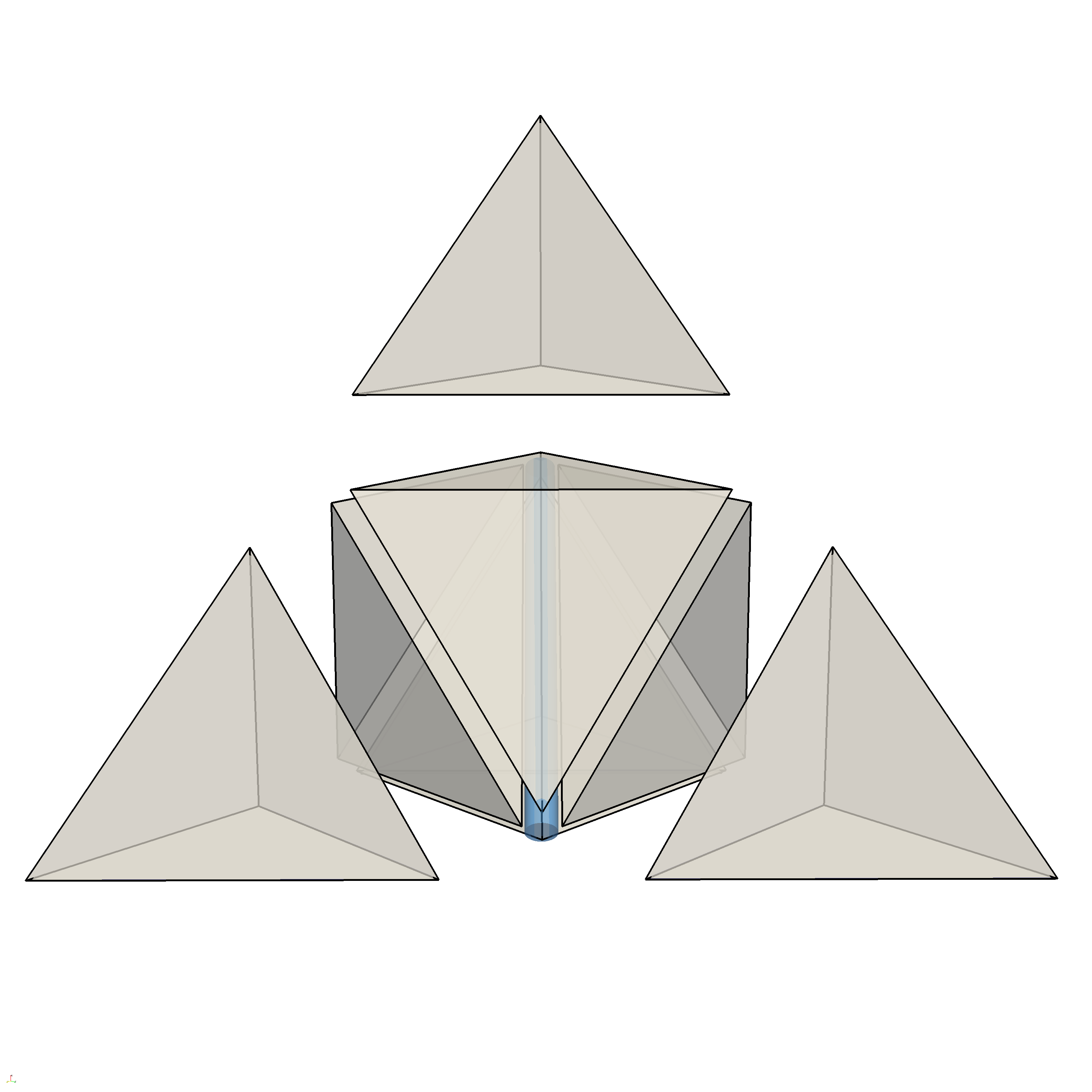
Figure 2: The uniform refinement of a coarse mesh tetrahedron yields eight fine mesh tetrahedra. Only the edge highlighted in blue does not lie entirely on the boundary of the tetrahedron.

The choice $[\mathbb{P}_{3}]^{3}-\mathbb{P}_{0}$ alleviates this problem of ill-posedness on the coarse cell and still satisfies $V_{H}\subset V_{h}$. However, as described in Section 2.1, this element is quite expensive without improving accuracy of the solution.

A much cheaper alternative is offered by the $[\mathbb{P}_{1}\oplus B^{F}_{3}]^{3}\mathrm{-}\mathbb{P}_{0}$ element. This does satisfy the inf-sup condition but violates $V_{H}\subset V_{h}$. The non-nestedness is demonstrated in Figure 3; a coarse bubble cannot be interpolated exactly by functions in $V_{h}$. In particular, the flux across the coarse grid faces is not preserved, hence violating (32).

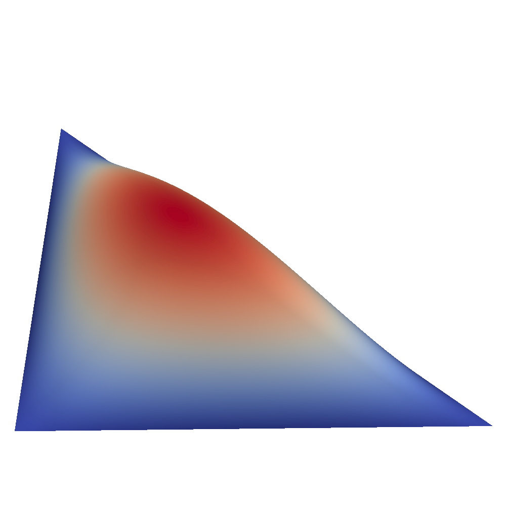
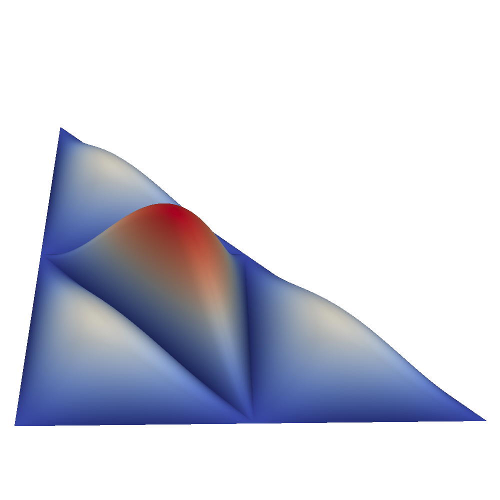
Figure 3: Left: Degrees of freedom on the facet of a coarse cell and its refinement. Middle: Bubble function on a coarse facet. Right: Prolongation of a bubble function.

A brief calculation shows that every coarse grid bubble is interpolated by four fine grid bubbles: one with coefficient $1$, the other three with coefficient $1/2$. From this it follows immediately that the integral of the prolonged bubble is equal to $(1+3\cdot\frac{1}{2})/4=\frac{5}{8}$ of the integral of the coarse bubble. Hence, when using a hierarchical basis, since the piecewise linear basis functions are prolonged exactly we can obtain a prolongation that satisfies (32) by simply multiplying the coefficients of the fine grid bubble functions by $8/5$. After this scaling, the local correction $w_{T}$ is computed as described above. For a nodal basis, a change of basis to the hierarchical basis should be performed.

This modification of the prolongation operator is crucial for the solver to work with the $[\mathbb{P}_{1}\oplus B^{F}_{3}]^{3}\mathrm{-}\mathbb{P}_{0}$ element. We demonstrate this by showing the residual of the outer flexible GMRES iteration for the linear solve in the first Newton step at $\mathrm{Re}=10$ for a lid-driven cavity problem (see section 5.5 for details) in Table 1. Without modifying the prolongation of the facet bubbles, we observe no convergence.

Iteration	Residual with bubble scaling	Residual without bubble scaling
0	$3.499\hphantom{{}\times 10^{+0}}$	$3.499$
1	$1.554\times 10^{-2}$	$3.499$
2	$1.716\times 10^{-3}$	$3.499$
3	$1.821\times 10^{-4}$	$3.496$
4	$1.651\times 10^{-5}$	$3.495$

Table 1: Residual of the outer flexible GMRES solver when employing the $[\mathbb{P}_{1}\oplus B^{F}_{3}]^{3}\mathrm{-}\mathbb{P}_{0}$ element. It is necessary to modify the prolongation operator to achieve convergence with this element.

Lastly, we consider the $[\mathbb{P}_{2}\oplus B^{F}_{3}]^{3}-\mathbb{P}_{0}$ element. While it is also non-nested, it turns out that the interpolation is exact on the facets of each coarse cell and hence flux preserving. To see this, observe that the cubic facet bubble function is only quadratic on the newly introduced edges of a regularly refined facet, as they are parallel to the edges of the coarse facet and therefore one of the barycentric coordinates is constant. The coarse bubble function is therefore prolonged exactly. This means that the $[\mathbb{P}_{2}\oplus B^{F}_{3}]^{3}-\mathbb{P}_{0}$ element can be used with the Schöberl prolongation operator (34), without the modifications necessary for $[\mathbb{P}_{1}\oplus B^{F}_{3}]^{3}\mathrm{-}\mathbb{P}_{0}$ described above. However, in our preliminary numerical experiments the simpler prolongation was outweighed by the cost of the larger number of degrees of degrees of freedom, and hence we use $[\mathbb{P}_{1}\oplus B^{F}_{3}]^{3}\mathrm{-}\mathbb{P}_{0}$ for the numerical experiments in section 5.

Remark .

Only the prolongation is modified; as in Benzi & Olshanskii [7], the natural operations are used for restriction and injection.

4.3 The advection terms

So far we have neglected the terms arising from the linearization of the advection term. Applying a Newton linearization, (20) becomes: find $u\in V_{h,0}$ such that

(39) $$(2\nu\varepsilon(u),\nabla v)+(w\cdot\nabla u,v)+(u\cdot\nabla w,v)+\gamma(\mathrm{P}_{Q_{h}}\nabla\cdot u,\nabla\cdot v)=(f,v)$$

for all $v\in V_{h,0}$, while the Picard linearization yields: find $u\in V_{h,0}$ such that

(40) $$(2\nu\varepsilon(u),\nabla v)+(w\cdot\nabla u,v)+\gamma(\mathrm{P}_{Q_{h}}\nabla\cdot u,\nabla\cdot v)=(f,v)$$

for all $v\in V_{h,0}$. The Picard linearization is easier to solve but sacrifices quadratic convergence of the nonlinear solver. Several authors have reported success with geometric multigrid for scalar analogues of (40) without the grad-div term, using a combination of line/plane relaxation and SUPG stabilization [65, 61, 81]. Olshanskii and Benzi [59] and Elman et al. [28] apply preconditioners built on the Picard linearization (40) to the Newton linearization (39), with good results.

Numerical experiments indicated that the additive star iteration alone was not effective as a relaxation method for (39). (Benzi and Olshanskii [7] used a multiplicative star iteration with multiple directional sweeps, but we wished to avoid this as its performance varies with the core count in parallel.) We investigated the multiplicative composition of additive star iterations and plane smoothers, and while this led to a successful multigrid cycle, the plane smoothers were quite expensive (involving many 2D solves) and were also difficult to parallelize on arbitrary unstructured grids where the parallel decomposition does not divide into planes. While the additive star iteration alone is not effective as a relaxation for (39), we found that a few iterations of GMRES preconditioned by the additive star iteration was surprisingly effective as a relaxation method, even for low viscosities. This point merits further analysis and will be considered in future work. This relaxation method also has the advantage that it is easy to parallelize, with convergence independent of the parallel decomposition.

5 Numerical results

5.1 Algorithm details

A graphical representation of the entire algorithm is shown in Figure 4. We employ simple continuation in Reynolds number as a globalization device, as Newton’s method is not globally convergent. Newton’s method is globalized with the $L^{2}$ line search algorithm of PETSc [21].

Figure 4: An outline of the algorithm for solving (1).

We use flexible GMRES [67] as the outermost solver for the linearized Newton system, as we employ GMRES in the multigrid relaxation. If the pressure is only defined up to a constant, then the appropriate nullspace is passed to the Krylov solver and the solution is orthogonalized against the nullspace at every iteration. We use the full block factorization preconditioner

(41) $$P^{-1}=\left(\begin{array}[]{cc}I&-\tilde{A}_{\gamma}^{-1}B^{T}\\ 0&I\\ \end{array}\right)\left(\begin{array}[]{cc}\tilde{A}_{\gamma}^{-1}&0\\ 0&\tilde{S}^{-1}\\ \end{array}\right)\left(\begin{array}[]{cc}I&0\\ -B\tilde{A}_{\gamma}^{-1}&I\\ \end{array}\right)$$

with approximate inner solves $\tilde{A}_{\gamma}^{-1}$ and $\tilde{S}^{-1}$ for the augmented momentum block and the Schur complement respectively. The diagonal, upper and lower triangular variants described in [58, 43] also converge well, but these took longer runtimes in preliminary experiments.

We use one application of a full multigrid cycle [16, Figure 1.2] using the components described in section 4 for $\tilde{A}_{\gamma}^{-1}$. The problem on each level is constructed by rediscretization; fine grid functions, such as the current iterate in the Newton scheme, are transferred to the coarse levels via injection. On each level the SUPG stabilization is performed with parameters corresponding to the mesh in question. For each relaxation sweep we perform 6 (in 2D) or 10 (in 3D) GMRES iterations preconditioned by the additive star iteration; at lower Reynolds numbers this can be reduced, but we found that these expensive smoothers represented the optimal tradeoff between inner and outer work at higher Reynolds numbers. The problem on the coarsest level is solved with the SuperLU_DIST sparse direct solver [54, 53]. For scalability, the coarse grid solve is agglomerated onto a single compute node using PETSc’s telescoping facility [57]. As all inner solvers are additive, the convergence of the solver is independent of the parallel decomposition (up to roundoff).

5.2 Software implementation

The solver proposed in the previous section is complex, and relies heavily on PETSc’s capability for the arbitrarily nested composition of solvers [20]. For the implementation of local patch solves, we have developed a new subspace correction preconditioner for PETSc that relies on the DMPlex unstructured mesh component [49, 50] for topological subspace construction and provides an extensible callback interface that allows for the very general specification of additive Schwarz methods. A detailed description of this preconditioner is in preparation.

5.3 Solver verification with the method of manufactured solutions

In order to verify the implementation and the convergence of the $[\mathbb{P}_{1}\oplus B^{F}_{3}]^{3}\mathrm{-}\mathbb{P}_{0}$ element we employ the method of manufactured solution. We start by considering the pressure and velocity field proposed in [73], which is rescaled to the $[0,2]^{2}$ square. This results in $u=(u_{1},u_{2})$ with

(42) $$u_{1}(x,y)= \ \frac{1}{4}(x-2)^{2}x^{2}y\left(y^{2}-2\right)$$

$$u_{2}(x,y)= \ -\frac{1}{4}x\left(x^{2}-3x+2\right)y^{2}\left(y^{2}-4\right)$$

$$\tilde{p}(x,y)= \ \frac{xy\left(3x^{4}-15x^{3}+10x^{2}y^{2}-30x\left(y^{2}-2\right)+20\left(y^{2}-2\right)\right)}{5\mathrm{Re}}$$

$$\ -\frac{1}{128}(x-2)^{4}x^{4}y^{2}\left(y^{4}-2y^{2}+8\right)$$

$$p(x,y)= \ \tilde{p}-\frac{1}{4}\int_{[0,2]^{2}}\tilde{p}(x,y)\ \mathrm{d}x=\tilde{p}+\frac{1408}{33075}-\frac{8}{5\mathrm{Re}}.$$

As we are primarily interested in the three dimensional case, we extend the vector field into the $z$ dimension via $u(x,y,z)=(u_{1}(x,y),u_{2}(x,y),0)$. The pressure remains the same as in two dimensions.

To demonstrate that the error convergence is independent of $\gamma$, we run the solver for values $\gamma=1$ and $\gamma=10^{4}$. Figure 5 shows the error between the computed velocity and pressure and their known analytical solutions for $\mathrm{Re}=1$, $\mathrm{Re}=200$ and $\mathrm{Re}=500$. Due to the DG0 discretization we expect, and see, first order convergence of the pressure. Without stabilization, we expect second order convergence for the velocity field; however, due to the presence of the SUPG stabilization this is reduced to linear convergence for coarse meshes. Once the mesh is fine enough so that $h^{-1}\gtrsim\mathrm{Re}$, second order convergence is recovered.

Figure 5: Convergence of the computed velocity and pressure field as the mesh is refined for a 3D lid-driven cavity test problem.

5.4 Two-dimensional experiments

We consider two representative benchmark problems: the regularized lid-driven cavity and backward-facing step problems, fully described in [30, examples 8.1.2 and 8.1.3]. For each experiment, we fix a coarse grid and vary the number of refinements to vary the size of the problem under consideration; all refinements are used in the multigrid iteration, to ensure that the convergence does not deteriorate as more levels are employed. We employ the $[\mathbb{P}_{2}]^{2}\mathrm{-}\mathbb{P}_{0}$ element for all two dimensional experiments. To investigate the performance of the solver with Reynolds number, the problem is first solved for $\mathrm{Re}=10$, then $\mathrm{Re}=100$, and then in steps of $100$ until $\mathrm{Re}=10000$, with the solution for the previous value of $\mathrm{Re}$ used as initial guess for the next. The Stokes equations are solved using a standard geometric multigrid algorithm with the pressure mass matrix as Schur complement approximation and point-block SOR as a smoother to provide the initial guess used at $\mathrm{Re}=10$. The augmented Lagrangian parameter is set to $\gamma=10^{4}$ in these and all subsequent experiments.

The linear solves are terminated with an absolute tolerance of $10^{-10}$ in the $\ell_{2}$-norm and a relative tolerance of $10^{-6}$. The nonlinear solves are terminated with an absolute tolerance of $10^{-8}$ and a relative tolerance of $10^{-10}$. As each outer iteration of the Krylov method does a fixed amount of work (i.e. all subproblems are solved with a fixed number of iterations, not to a specified tolerance), the solver scales well with mesh size and Reynolds number if the iteration counts remain approximately constant.

For comparison, we solve the same problems using the reference implementations of the PCD and LSC preconditioners in version 3.5 of IFISS [29], up to $\mathrm{Re}=1000$, as IFISS does not employ stabilization of the advection term. For both of these preconditioners we use the variant that takes corrections for the boundary conditions into account and we solve the inner problems in the Schur complement approximation using an algebraic multigrid solver. We employ the hybrid strategy suggested by [30, p. 391] that uses a single sweep of ILU(0) on the finest level and two iterations of point-damped Jacobi for pre- and post-smoothing on all coarsened levels. A relative tolerance of $10^{-6}$ is set for the Krylov solver and an absolute tolerance of $10^{-8}$ for the Newton solver.

We begin by considering the regularized lid-driven cavity problem. The coarse grid used is the $16\times 16$ grid of triangles of negative slope. The results are shown in Table 2; we observe only very mild iteration growth from $\mathrm{Re}=10$ to $\mathrm{Re}=10000$ with the performance improving as more refinements are taken. Iteration counts using the PCD and LSC preconditioners are shown in Table 3. For both PCD and LSC iteration counts increase substantially from $\mathrm{Re}=10$ to $\mathrm{Re}=1000$.

# refinements	# degrees of freedom	Reynolds number
		10	100	1000	5000	10000
1	$1.0\times 10^{4}$	2.50	4.33	6.00	8.00	14.00
2	$4.1\times 10^{4}$	2.50	3.33	6.67	8.50	10.00
3	$1.6\times 10^{5}$	2.50	3.00	5.67	8.50	9.00
4	$6.6\times 10^{5}$	2.50	2.67	5.00	8.00	8.50

Table 2: Average number of outer Krylov iterations per Newton step for the 2D regularized lid-driven cavity problem.

$1/h$	# degrees of freedom	Reynolds number
		10	100	1000
$2^{4}$	$8.34\times 10^{2}$	22.0/21.5	40.4/48.7	103.3/130.7
$2^{5}$	$3.20\times 10^{3}$	23.0/22.0	41.3/52.7	137.7/185.3
$2^{6}$	$1.25\times 10^{4}$	24.5/22.5	42.0/49.3	157.0/205.7
$2^{7}$	$4.97\times 10^{4}$	25.5/21.0	42.7/43.3	149.0/207.3
$2^{8}$	$1.98\times 10^{5}$	26.0/23.0	44.0/38.0	137.0/180.0

Table 3: Average number of outer Krylov iterations per Newton step for the 2D regularized lid-driven cavity problem with PCD/LSC preconditioner.

For the backward-facing step we observe that the performance is dependent on the resolution of the coarse grid. We consider two experiments, one starting with a coarse grid consisting of 6941 vertices and 13880 elements (labeled A) and one consisting of 30322 vertices and 60642 elements (labeled B). Both unstructured triangular meshes were generated with Gmsh [33]. For mesh A, we observe that the iteration counts for large Reynolds numbers show the solver degrades somewhat as the mesh is refined, see Table 4. Using the finer coarse grid B alleviates this problem. The bottom half of Table 4 shows that iteration counts only approximately double as we increase from $\mathrm{Re}=10$ to $\mathrm{Re}=10000$.

# refinements	# degrees of freedom	Reynolds number
		10	100	1000	5000	10000
coarse grid A
1	$2.7\times 10^{5}$	3.00	4.00	5.50	12.00	26.50
2	$1.1\times 10^{6}$	2.67	4.50	5.50	11.50	31.50
3	$4.3\times 10^{6}$	4.00	7.00	6.00	14.00	21.00
coarse grid B
1	$1.2\times 10^{6}$	2.67	3.75	5.00	7.00	9.00
2	$4.8\times 10^{6}$	4.00	3.75	5.00	6.50	7.00
3	$1.9\times 10^{7}$	3.67	5.75	5.50	5.00	5.50

Table 4: Average number of outer Krylov iterations per Newton step for the 2D backward-facing step problem for two different coarse grids.

The results for PCD and LSC on the backwards-facing step are shown in Table 5. The iteration counts approximately treble as we increase from $\mathrm{Re}=10$ to $\mathrm{Re}=1000$.

$1/h$	# degrees of freedom	Reynolds number
		10	100	1000
$2^{4}$	$3.94\times 10^{3}$	23.0/29.0	32.5/47.5	NaNF/NaNF
$2^{5}$	$1.52\times 10^{4}$	23.5/26.0	31.0/45.0	221.3/329.0
$2^{6}$	$5.96\times 10^{4}$	23.5/25.5	30.5/42.8	122.7/225.7
$2^{7}$	$2.36\times 10^{5}$	23.5/25.5	30.0/40.8	85.3/161.3
$2^{8}$	$9.38\times 10^{5}$	23.5/27.0	30.0/40.0	78.3/128.0

Table 5: Average number of outer Krylov iterations per Newton step for the 2D backwards-facing step problem with PCD/LSC preconditioner. NaNF denotes failure due to NaNs occurring in the solve for the velocity block.

5.4.1 Runtime comparison to SIMPLE

To give some measure of the runtime of the solver, we compare it to an implementation of SIMPLE [63, Section 6.7] in the same software framework. We select the lid-driven cavity in two dimensions with three refinements ($1.6\times 10^{5}$ degrees of freedom) as a representative problem. The SIMPLE preconditioner is given by

(43) $$P_{\text{SIMPLE}}^{-1}=\left(\begin{array}[]{cc}I&-\operatorname{diag}(A)^{-1}B^{T}\\ 0&I\\ \end{array}\right)\left(\begin{array}[]{cc}\tilde{A}^{-1}&0\\ 0&\tilde{S}_{\text{SIMPLE}}^{-1}\\ \end{array}\right)\left(\begin{array}[]{cc}I&0\\ -B\tilde{A}^{-1}&I\\ \end{array}\right),$$

where

(44) $$\tilde{S}_{\text{SIMPLE}}=-B^{T}\operatorname{diag}(A)^{-1}B$$

and no grad-div augmentation is employed. $\tilde{A}^{-1}$ is approximated by one full multigrid cycle of the ML algebraic multigrid library [32]; $\tilde{S}_{\text{SIMPLE}}^{-1}$ is approximated with one V cycle of ML.

Reynolds number	Augmented Lagrangian		SIMPLE
	Total iterations	Time (min)	Total iterations	Time (min)
10	4	0.21	515	1.06
50	6	0.30	741	1.57
100	8	0.38	979	2.01
150	10	0.46	1111	2.27
200	10	0.46	1185	2.48

Table 6: Iteration count and runtime comparison against the SIMPLE preconditioner.

The results for several continuation steps are shown in Table 6. The computations were performed in serial. Each SIMPLE iteration is approximately 22–26 times faster than an augmented Lagrangian iteration, but the lower cost per iteration is outweighed by the greater number of iterations required.

5.5 Three-dimensional experiments

The lid-driven cavity and backward-facing step problems can both be extended to three dimensions in a natural way. For the lid-driven cavity, we consider the cube $\Omega=[0,2]^{3}$ with no-slip boundary conditions on all sides apart from the top boundary $\{y=2\}$. On the top boundary we enforce $u(x,y,z)=(x^{2}(2-x)^{2}z^{2}(2-z)^{2},0,0)^{T}$. The three dimensional backwards-facing step is given by $\Omega=\left(\left([0,10]\times[1,2]\right)\cup\left([1,10]\times[0,1]\right)\right)\times[0,1]$. We enforce the inflow condition $u(x,y,z)=(4(2-y)(y-1)z(1-z),0,0)^{T}$ on the left boundary $\{x=0\}$, a natural outflow condition on the right boundary $\{x=10\}$ and no-slip boundary conditions on the remaining boundaries.

Two aspects of the solver were modified compared to the version used in two dimensions. Firstly, we observe that reducing the size of the SUPG stabilization by a factor of $1/20$ improves convergence significantly. Secondly, the relative tolerance for the linear solver was relaxed to $10^{-5}$ and the absolute tolerance for the linear and the nonlinear solver was relaxed to $10^{-8}$, to save computational time. The three-dimensional experiments were both run for $[\mathbb{P}_{1}\oplus B^{F}_{3}]^{3}\mathrm{-}\mathbb{P}_{0}$ discretizations of up to one billion degrees of freedom on ARCHER, the UK national supercomputer. The runs were terminated at $\mathrm{Re}=5000$ due to budgetary constraints. Images of the solutions are shown in Figures 6 and 7.

# refinements	# degrees of freedom	Reynolds number
		10	100	1000	2500	5000
1	$2.1\times 10^{6}$	4.50	4.00	5.00	4.50	4.00
2	$1.7\times 10^{7}$	4.50	4.33	4.50	4.00	4.00
3	$1.3\times 10^{8}$	4.50	4.33	4.00	3.50	7.00
4	$1.1\times 10^{9}$	4.50	3.66	3.00	5.00	5.00

Table 7: Average number of outer Krylov iterations per Newton step for the 3D regularized lid-driven cavity problem.

# refinements	# degrees of freedom	Reynolds number
		10	100	1000	2500	5000
1	$2.1\times 10^{6}$	4.50	4.00	4.00	4.50	7.50
2	$1.7\times 10^{7}$	5.00	4.00	3.33	4.00	10.00
3	$1.3\times 10^{8}$	6.50	4.50	3.50	3.00	8.00
4	$1.0\times 10^{9}$	7.50	3.50	2.50	3.00	6.00

Table 8: Average number of outer Krylov iterations per Newton step for the 3D backwards-facing step problem.

As for the two-dimensional case, we see only very little variation of the iteration counts with Reynolds number over this range.

To stress the solver further, the lid-driven cavity with 2 refinements ($1.7\times 10^{7}$ degrees of freedom) was run until failure. Iteration counts remain stable until $\mathrm{Re}=7000$, then begin to increase, with eventual failure of convergence at $\mathrm{Re}=7700$.

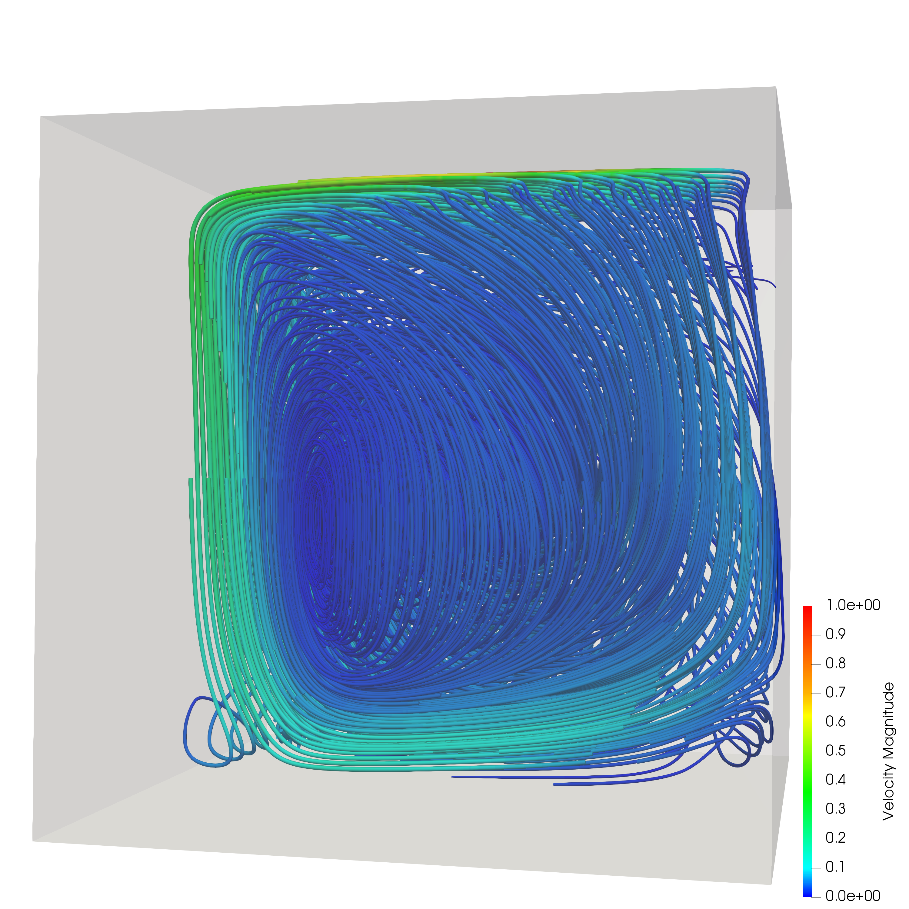
Figure 6: Interior view of the streamtubes of the 3D lid-driven cavity at $\mathrm{Re}=5000$. The color denotes speed.

Figure 7: Interior view of the streamtubes of the 3D backwards-facing step at $\mathrm{Re}=1000$. The color denotes speed.

5.5.1 Computational performance

Having seen that the algorithmic scalability of the solver is good, with well-controlled iteration counts, we now consider the computational performance. In Figures 8(a) and 8(b) we show the weak scaling of the total time to solution over all continuation steps. Both problems show excellent scalability from 48 to 24576 MPI processes, with the lid-driven cavity achieving a scaling efficiency of 80% and the backwards-facing step 79%. We attribute the lack of perfect scalability primarily to load imbalance in our mesh distribution. In both problems, although the mesh has a well-balanced partition of cells, for the patch smoother to have perfect load balance the number of vertices owned by each process must also be equal. The partitioning scheme used does not take this constraint into account, and we observe that the number of patches per process varies by a factor of 4 over the partition for the largest problems. The scaling and computational performance of the code will be improved in future work.

(a) Weak scaling of the three-dimensional lid-driven cavity.

(b) Weak scaling of the three-dimensional backwards-facing step.

Figure 8: Weak scaling of time to solution over all continuation steps for both 3D problems.

6 Conclusions and outlook

In this paper we have extended the multigrid method of Benzi, Olshanskii and Schöberl for the augmented momentum solve arising in the augmented Lagrangian preconditioner to three dimensions. The prolongation operator proposed by Schöberl works for the $[\mathbb{P}_{3}]^{3}\mathrm{-}\mathbb{P}_{0}$ and $[\mathbb{P}_{2}\oplus B^{F}_{3}]^{3}\mathrm{-}\mathbb{P}_{0}$ discretizations, while a modification is required to use the cheaper $[\mathbb{P}_{1}\oplus B^{F}_{3}]^{3}\mathrm{-}\mathbb{P}_{0}$ element. We have developed a new patchwise preconditioner in PETSc and implemented the resulting scheme in Firedrake. We have demonstrated iteration counts that grow very slowly with respect to the Reynolds number in both 2D and 3D for problems of up to a billion degrees of freedom. The code is freely available as open source.

However, this multigrid method is currently tightly coupled to the use of piecewise constant elements for the pressure for full robustness, and the discretizations considered here do not represent the divergence-free constraint exactly, which is highly desirable [44]. The key next step is to develop a Reynolds-robust preconditioner for these discretizations, such as the Scott–Vogelius element [70], the Guzmán–Neilan modification of Bernardi–Raugel [36], or a $H(\mathrm{div})$-conforming element [23]. It may also be possible to use this solver as a preconditioner for other discretisations, in a similar manner to the modified multigrid schemes studied in [45].

Code availability

For reproducibility, we cite archives of the exact software versions used to produce the results in this paper. All major Firedrake components have been archived on Zenodo [82]. An installation of Firedrake with components matching those used to produce the results in this paper can by obtained following the instructions at https://www.firedrakeproject.org/download.html with

export PETSC_CONFIGURE_OPTIONS="--download-superlu --download-superlu_dist \
   --with-cxx-dialect=C++11"
python3 firedrake-install --doi 10.5281/zenodo.3247427

The additive Schwarz preconditioner has been incorporated into PETSc as of version 3.10. The Navier–Stokes solver, and example files, are available at https://bitbucket.org/pefarrell/fmwns/, the version used in the paper is archived as part of [82].

References

- [1] M. S. Alnæs, A. Logg, K. B. Ølgaard, M. E. Rognes, and G. N. Wells, Unified Form Language: A domain-specific language for weak formulations of partial differential equations, ACM Transactions on Mathematical Software, 40 (2014), pp. 9:1–9:37, https://doi.org/10.1145/2566630.
- [2] D. N. Arnold, R. Falk, and R. Winther, Preconditioning in and applications, Mathematics of Computation, 66 (1997), pp. 957–984, https://doi.org/10.1090/S0025-5718-97-00826-0.
- [3] D. N. Arnold, R. S. Falk, and R. Winther, Multigrid in and , Numerische Mathematik, 85 (2000), pp. 197–217, https://doi.org/10.1007/pl00005386.
- [4] C. Bacuta, A unified approach for Uzawa algorithms, SIAM Journal on Numerical Analysis, 44 (2006), pp. 2633–2649, https://doi.org/10.1137/050630714.
- [5] S. Balay, S. Abhyankar, M. F. Adams, J. Brown, P. Brune, K. Buschelman, L. Dalcin, V. Eijkhout, W. D. Gropp, D. Kaushik, M. G. Knepley, L. C. McInnes, K. Rupp, B. F. Smith, S. Zampini, H. Zhang, and H. Zhang, PETSc users manual, Tech. Report ANL-95/11 - Revision 3.8, Argonne National Laboratory, 2017, http://www.mcs.anl.gov/petsc.
- [6] M. Benzi, G. H. Golub, and J. Liesen, Numerical solution of saddle point problems, Acta Numerica, 14 (2005), pp. 1–137, https://doi.org/10.1017/S0962492904000212.
- [7] M. Benzi and M. A. Olshanskii, An augmented Lagrangian-based approach to the Oseen problem, SIAM Journal on Scientific Computing, 28 (2006), pp. 2095–2113, https://doi.org/10.1137/050646421.
- [8] M. Benzi and M. A. Olshanskii, Field-of-values convergence analysis of augmented Lagrangian preconditioners for the linearized Navier–Stokes problem, SIAM Journal of Numerical Analysis, 49 (2011), pp. 770–788.
- [9] M. Benzi, M. A. Olshanskii, and Z. Wang, Modified augmented Lagrangian preconditioners for the incompressible Navier-Stokes equations, International Journal for Numerical Methods in Fluids, 66 (2011), pp. 486–508, https://doi.org/10.1002/fld.2267.
- [10] C. Bernardi and G. Raugel, Analysis of some finite elements for the Stokes problem, Mathematics of Computation, 44 (1985), p. 71, https://doi.org/10.2307/2007793.
- [11] C. Bernardi and G. Raugel, A conforming finite element method for the time-dependent navier–stokes equations, SIAM Journal on Numerical Analysis, 22 (1985), pp. 455–473.
- [12] D. Boffi, F. Brezzi, and M. Fortin, Finite elements for the Stokes problem, in Mixed Finite Elements, Compatibility Conditions, and Applications, D. Boffi and L. Gastaldi, eds., Lecture Notes in Mathematics, Springer, 2008, pp. 45–100.
- [13] D. Boffi and C. Lovadina, Analysis of new augmented Lagrangian formulations for mixed finite element schemes, Numerische Mathematik, 75 (1997), pp. 405–419, https://doi.org/10.1007/s002110050246.
- [14] S. Börm and S. L. Borne, -LU factorization in preconditioners for augmented Lagrangian and grad-div stabilized saddle point systems, International Journal for Numerical Methods in Fluids, 68 (2010), pp. 83–98, https://doi.org/10.1002/fld.2495.
- [15] D. Braess and R. Sarazin, An efficient smoother for the Stokes problem, Applied Numerical Mathematics, 23 (1997), pp. 3–19, https://doi.org/10.1016/s0168-9274(96)00059-1.
- [16] A. Brandt and O. E. Livne, Multigrid Techniques: 1984 Guide with Applications to Fluid Dynamics, vol. 67 of Classics in Applied Mathematics, SIAM, 2nd ed., 2011.
- [17] S. C. Brenner and L. R. Scott, The Mathematical Theory of Finite Element Methods, vol. 15 of Texts in Applied Mathematics, Springer-Verlag New York, third edition ed., 2008.
- [18] F. Brezzi and M. Fortin, Mixed and Hybrid Finite Element Methods, vol. 15 of Springer Series in Computational Mathematics, Springer New York, 1991, https://doi.org/10.1007/978-1-4612-3172-1, https://doi.org/10.1007%2F978-1-4612-3172-1.
- [19] A. N. Brooks and T. J. R. Hughes, Streamline upwind/Petrov-Galerkin formulations for convection dominated flows with particular emphasis on the incompressible Navier-Stokes equations, Computer Methods in Applied Mechanics and Engineering, 32 (1982), pp. 199–259, https://doi.org/10.1016/0045-7825(82)90071-8.
- [20] J. Brown, M. Knepley, D. May, L. McInnes, and B. Smith, Composable linear solvers for multiphysics, in 2012 11th International Symposium on Parallel and Distributed Computing (ISPDC), 2012, pp. 55–62, https://doi.org/10.1109/ISPDC.2012.16.
- [21] P. R. Brune, M. G. Knepley, B. F. Smith, and X. Tu, Composing scalable nonlinear algebraic solvers, SIAM Review, 57 (2015), pp. 535–565, https://doi.org/10.1137/130936725.
- [22] A. J. Chorin, A numerical method for solving incompressible viscous flow problems, Journal of Computational Physics, 2 (1967), pp. 12–26, https://doi.org/10.1016/0021-9991(67)90037-x.
- [23] B. Cockburn, G. Kanschat, and D. Schötzau, A note on discontinuous Galerkin divergence-free solutions of the Navier–Stokes equations, Journal of Scientific Computing, 31 (2006), pp. 61–73, https://doi.org/10.1007/s10915-006-9107-7.
- [24] A. C. de Niet and F. W. Wubs, Two preconditioners for saddle point problems in fluid flows, International Journal for Numerical Methods in Fluids, 54 (2007), pp. 355–377, https://doi.org/10.1002/fld.1401.
- [25] M. Eiermann and O. G. Ernst, Geometric aspects of the theory of Krylov subspace methods, Acta Numerica, 10 (2001), https://doi.org/10.1017/S0962492901000046.
- [26] H. Elman, V. E. Howle, J. Shadid, R. Shuttleworth, and R. Tuminaro, Block preconditioners based on approximate commutators, SIAM Journal on Scientific Computing, 27 (2006), pp. 1651–1668, https://doi.org/10.1137/040608817.
- [27] H. Elman and D. Silvester, Fast nonsymmetric iterations and preconditioning for Navier–Stokes equations, SIAM Journal on Scientific Computing, 17 (1996), pp. 33–46, https://doi.org/10.1137/0917004.
- [28] H. C. Elman, D. Loghin, and A. J. Wathen, Preconditioning techniques for Newton's method for the incompressible Navier–Stokes equations, BIT Numerical Mathematics, 43 (2003), pp. 961–974, https://doi.org/10.1023/b:bitn.0000014565.86918.df.
- [29] H. C. Elman, A. Ramage, and D. J. Silvester, IFISS: A computational laboratory for investigating incompressible flow problems, SIAM Review, 56 (2014), pp. 261–273, https://doi.org/10.1137/120891393.
- [30] H. C. Elman, D. J. Silvester, and A. J. Wathen, Finite Elements and Fast Iterative Solvers: with applications in incompressible fluid dynamics, Oxford University Press, 2014.
- [31] M. Fortin and R. Glowinski, Augmented Lagrangian Methods: Applications to the Numerical Solution of Boundary-Value Problems, vol. 15 of Studies in Mathematics and Its Applications, Elsevier Science Ltd, 1983.
- [32] M. Gee, C. Siefert, J. Hu, R. Tuminaro, and M. Sala, ML 5.0 smoothed aggregation user’s guide, Tech. Report SAND2006-2649, Sandia National Laboratories, 2006.
- [33] C. Geuzaine and J.-F. Remacle, Gmsh: A 3-D finite element mesh generator with built-in pre- and post-processing facilities, International Journal for Numerical Methods in Engineering, 79 (2009), pp. 1309–1331, https://doi.org/10.1002/nme.2579.
- [34] V. Girault and P.-A. Raviart, Finite Element Methods for Navier-Stokes Equations: Theory and Algorithms, vol. 5 of Springer Series in Computational Mathematics, Springer, 1986.
- [35] A. Greenbaum, V. Pták, and Z. Strakoš, Any nonincreasing convergence curve is possible for GMRES, SIAM Journal on Matrix Analysis and Applications, 17 (1996), pp. 465–469, https://doi.org/10.1137/S0895479894275030.
- [36] J. Guzmán and M. Neilan, Inf-sup stable finite elements on barycentric refinements producing divergence–free approximations in arbitrary dimensions, 2017, https://arxiv.org/abs/1710.08044.
- [37] S. Hamilton, M. Benzi, and E. Haber, New multigrid smoothers for the Oseen problem, Numerical Linear Algebra with Applications, (2010), https://doi.org/10.1002/nla.707.
- [38] X. He, M. Neytcheva, and S. S. Capizzano, On an augmented Lagrangian-based preconditioning of Oseen type problems, BIT Numerical Mathematics, 51 (2011), pp. 865–888, https://doi.org/10.1007/s10543-011-0334-4.
- [39] X. He, C. Vuik, and C. M. Klaij, Combining the augmented lagrangian preconditioner with the simple schur complement approximation, SIAM Journal on Scientific Computing, 40 (2018), pp. A1362–A1385.
- [40] T. Heister and G. Rapin, Efficient augmented Lagrangian-type preconditioning for the Oseen problem using grad-div stabilization, International Journal for Numerical Methods in Fluids, 71 (2012), pp. 118–134, https://doi.org/10.1002/fld.3654.
- [41] R. Hiptmair, Multigrid method for in three dimensions, Electronic Transactions on Numerical Analysis, 6 (1997), pp. 133–152.
- [42] M. Homolya, L. Mitchell, F. Luporini, and D. A. Ham, TSFC: a structure-preserving form compiler, SIAM Journal on Scientific Computing, 40 (2018), pp. C401–C428, https://doi.org/10.1137/17M1130642, https://arxiv.org/abs/1705.03667.
- [43] I. C. F. Ipsen, A note on preconditioning nonsymmetric matrices, SIAM Journal on Scientific Computing, 23 (2001), pp. 1050–1051, https://doi.org/10.1137/S1064827500377435.
- [44] V. John, A. Linke, C. Merdon, M. Neilan, and L. G. Rebholz, On the divergence constraint in mixed finite element methods for incompressible flows, SIAM Review, 59 (2017), pp. 492–544, https://doi.org/10.1137/15m1047696.
- [45] V. John and G. Matthies, Higher-order finite element discretizations in a benchmark problem for incompressible flows, International Journal for Numerical Methods in Fluids, 37 (2001), pp. 885–903, https://doi.org/10.1002/fld.195.
- [46] D. Kay, D. Loghin, and A. Wathen, A preconditioner for the steady-state Navier–Stokes equations, SIAM Journal on Scientific Computing, 24 (2002), pp. 237–256, https://doi.org/10.1137/S106482759935808X.
- [47] R. C. Kirby, Algorithm 839: FIAT, a new paradigm for computing finite element basis functions, ACM Transactions on Mathematical Software, 30 (2004), pp. 502–516, https://doi.org/10.1145/1039813.1039820.
- [48] R. C. Kirby and L. Mitchell, Solver composition across the PDE/linear algebra barrier, SIAM Journal on Scientific Computing, 40 (2018), pp. C76–C98, https://doi.org/10.1137/17M1133208, https://arxiv.org/abs/1706.01346.
- [49] M. G. Knepley and D. A. Karpeev, Flexible representation of computational meshes, Tech. Report ANL/MCS-P1295-1005, Argonne National Laboratory, 2005.
- [50] M. G. Knepley and D. A. Karpeev, Mesh Algorithms for PDE with Sieve I: Mesh Distribution, Scientific Programming, 17 (2009), pp. 215–230, https://doi.org/10.1155/2009/948613.
- [51] G. M. Kobel’kov, On solving the Navier-Stokes equations at large Reynolds numbers, Russian Journal of Numerical Analysis and Mathematical Modelling, 10 (1995), https://doi.org/10.1515/rnam.1995.10.1.33.
- [52] Y.-J. Lee, J. Wu, J. Xu, and L. Zikatanov, Robust subspace correction methods for nearly singular systems, Mathematical Models and Methods in Applied Sciences, 17 (2007), pp. 1937–1963, https://doi.org/10.1142/s0218202507002522.
- [53] X. S. Li and J. W. Demmel, SuperLU_DIST: A scalable distributed-memory sparse direct solver for unsymmetric linear systems, ACM Transactions on Mathematical Software, 29 (2003), pp. 110–140.
- [54] X. S. Li, J. W. Demmel, J. R. Gilbert, iL. Grigori, M. Shao, and I. Yamazaki, SuperLU Users’ Guide, Tech. Report LBNL-44289, Lawrence Berkeley National Laboratory, September 1999.
- [55] D. Loghin and A. J. Wathen, Analysis of preconditioners for saddle-point problems, SIAM Journal on Scientific Computing, 25 (2004), pp. 2029–2049, https://doi.org/10.1137/S1064827502418203.
- [56] K.-A. Mardal and R. Winther, Preconditioning discretizations of systems of partial differential equations, Numerical Linear Algebra with Applications, 18 (2011), pp. 1–40, https://doi.org/10.1002/nla.716.
- [57] D. A. May, P. Sanan, K. Rupp, M. G. Knepley, and B. F. Smith, Extreme-scale multigrid components within PETSc, in Proceedings of the Platform for Advanced Scientific Computing Conference, 2016, https://doi.org/10.1145/2929908.2929913.
- [58] M. F. Murphy, G. H. Golub, and A. J. Wathen, A note on preconditioning for indefinite linear systems, SIAM Journal on Scientific Computing, 21 (2000), pp. 1969–1972, https://doi.org/10.1137/S1064827599355153.
- [59] M. A. Olshanskii and M. Benzi, An augmented Lagrangian approach to linearized problems in hydrodynamic stability, SIAM Journal on Scientific Computing, 30 (2008), pp. 1459–1473, https://doi.org/10.1137/070691851.
- [60] M. A. Olshanskii and A. Reusken, Grad-div stablilization for Stokes equations, Mathematics of Computation, 73 (2003), pp. 1699–1719, https://doi.org/10.1090/s0025-5718-03-01629-6.
- [61] M. A. Olshanskii and A. Reusken, Convergence analysis of a multigrid method for a convection-dominated model problem, SIAM Journal on Numerical Analysis, 42 (2004), pp. 1261–1291, https://doi.org/10.1137/s0036142902418679.
- [62] M. A. Olshanskii and E. E. Tyrtyshnikov, Iterative Methods for Linear Systems: Theory and Applications, SIAM, 2014.
- [63] S. Patankar, Numerical Heat Transfer and Fluid Flow, Hemisphere Series on Computational Methods in Mechanics and Thermal Science, Taylor & Francis, 1 ed., 1980.
- [64] A. Quarteroni and A. Valli, Numerical Approximation of Partial Differential Equations, vol. 23 of Springer Series in Computational Mathematics, Springer, 2008.
- [65] A. Ramage, A multigrid preconditioner for stabilised discretisations of advection–diffusion problems, Journal of Computational and Applied Mathematics, 110 (1999), pp. 187–203, https://doi.org/10.1016/s0377-0427(99)00234-4.
- [66] F. Rathgeber, D. A. Ham, L. Mitchell, M. Lange, F. Luporini, A. T. T. Mcrae, G.-T. Bercea, G. R. Markall, and P. H. J. Kelly, Firedrake: automating the finite element method by composing abstractions, ACM Transactions on Mathematical Software, 43 (2016), pp. 1–27, https://doi.org/10.1145/2998441.
- [67] Y. Saad, A flexible inner-outer preconditioned GMRES algorithm, SIAM Journal on Scientific Computing, 14 (1993), pp. 461–469, https://doi.org/10.1137/0914028.
- [68] J. Schöberl, Multigrid methods for a parameter dependent problem in primal variables, Numerische Mathematik, 84 (1999), pp. 97–119, https://doi.org/10.1007/s002110050465.
- [69] J. Schöberl, Robust Multigrid Methods for Parameter Dependent Problems, PhD thesis, Johannes Kepler Universität Linz, Linz, Austria, 1999.
- [70] L. R. Scott and M. Vogelius, Norm estimates for a maximal right inverse of the divergence operator in spaces of piecewise polynomials, ESAIM: Mathematical Modelling and Numerical Analysis, 19 (1985), pp. 111–143.
- [71] L. R. Scott and S. Zhang, Finite element interpolation of nonsmooth functions satisfying boundary conditions, Mathematics of Computation, 54 (1990), pp. 483–493, http://www.jstor.org/stable/2008497.
- [72] F. Shakib, T. J. R. Hughes, and Z. Johan, A new finite element formulation for computational fluid dynamics: X. The compressible Euler and Navier-Stokes equations, Computer Methods in Applied Mechanics and Engineering, 89 (1991), pp. 141–219, https://doi.org/10.1016/0045-7825(91)90041-4.
- [73] T. Shih, C. Tan, and B. Hwang, Effects of grid staggering on numerical schemes, International Journal for Numerical Methods in Fluids, 9 (1989), pp. 193–212.
- [74] D. Silvester and A. J. Wathen, Fast iterative solution of stabilised Stokes systems. Part II: Using general block preconditioners, SIAM Journal on Numerical Analysis, 31 (1994), pp. 1352–1367, https://doi.org/10.1137/0731070.
- [75] G. Starke, Field-of-values analysis of preconditioned iterative methods for nonsymmetric elliptic problems, Numerische Mathematik, 78 (1997), pp. 103–117, https://doi.org/10.1007/s002110050306.
- [76] R. Temam, Une méthode d’approximation de la solution des équations de Navier-Stokes, Bulletin de la Société Mathématique de France, 98 (1968), pp. 115–152.
- [77] S. Turek, Efficient Solvers for Incompressible Flow Problems: An Algorithmic and Computational Approach, Lecture Notes in Computational Science and Engineering, Springer, 1999.
- [78] M. ur Rehman, C. Vuik, and G. Segal, A comparison of preconditioners for incompressible Navier-Stokes solvers, International Journal for Numerical Methods in Fluids, 57 (2008), pp. 1731–1751, https://doi.org/10.1002/fld.1684.
- [79] S. P. Vanka, Block-implicit multigrid solution of Navier-Stokes equations in primitive variables, Journal of Computational Physics, 65 (1986), pp. 138–158, https://doi.org/10.1016/0021-9991(86)90008-2.
- [80] A. J. Wathen, Preconditioning, Acta Numerica, 24 (2015), pp. 329–376, https://doi.org/10.1017/S0962492915000021.
- [81] C.-T. Wu and H. C. Elman, Analysis and comparison of geometric and algebraic multigrid for convection-diffusion equations, SIAM Journal on Scientific Computing, 28 (2006), pp. 2208–2228, https://doi.org/10.1137/060662940.
- [82] Software used in ’An augmented Lagrangian preconditioner for the 3D stationary incompressible Navier–Stokes equations at high Reynolds number’, Jun 2019, https://doi.org/10.5281/zenodo.3247427.