Screening in the finite-temperature reduced Hartree-Fock model

Abstract.

We prove the existence of solutions of the reduced Hartree-Fock equations at finite temperature for a periodic crystal with a small defect, and show total screening of the defect charge by the electrons. We also show the convergence of the damped self-consistent field iteration using Kerker preconditioning to remove charge sloshing. As a crucial step of the proof, we define and study the properties of the dielectric operator.

1. Introduction

A point charge $Q$ placed in vacuum creates an electric potential $\frac{Q}{4\pi r}$, $r$ being the distance to the charge (in units where the permittivity of the vacuum $\varepsilon_{0}$ is taken to be $1$). By contrast, when an defect is placed in a material, the material reorganises itself: a positive charge creates an energetically favorable region for the electrons, which flock towards the defect. At equilibrium, they form a “shield” of negative charge, effectively screening the Coulomb interaction at long range.

Phenomenologically, insulators and metals exhibit a different screening behavior. In insulators, electrons are tightly bound to the nuclei, and cannot deviate too much from their equilibrium position to move towards the defect. Accordingly, the long-range behavior of the total potential, including the effects of the electrons, is $Q/(4\pi\varepsilon r)$, where $\varepsilon>1$ is the dielectric constant of the material. Thus, effectively, the charge $Q$ is scaled by the dielectric constant $\varepsilon$: this is called partial screening.

In metals, however, electrons are free to move in response to the defect and totally screen it, so that the total potential becomes effectively short-range. A simple model for the total potential is the Yukawa potential

$$V(x)=\frac{Qe^{-k|x|}}{|x|}$$

where $1/k$ is the screening length. At low temperatures however, $V$ displays an oscillatory behavior with a power-law decay, called Friedel oscillations.

The purpose of this paper is to justify the total screening of small defects in the reduced Hartree-Fock (rHF) model at finite temperature. This is to be contrasted with the partial screening of insulators at zero temperature obtained in [7] in the same model: at finite temperature, electrons are mobile and behave as in a metal. We also justify the Kerker preconditioning scheme, which neutralizes the “charge sloshing” effect that slows down simple self-consistent iterations in extended systems [15].

For a finite system of $N_{\rm el}$ electrons in an external potential $V_{\rm ext}$, the reduced Hartree-Fock (rHF) equation for the total potential $V$ is given by

$$\begin{cases}V=V_{\rm ext}+{v_{\rm c}}F_{\varepsilon_{F}}(V),\\ \int_{\mathbb{R}^{3}}F_{\varepsilon_{F}}(V)=N_{\rm el}.\end{cases}$$

The Coulomb operator ${v_{\rm c}}$ is given by the convolution

$$({v_{\rm c}}\rho)(x)=\frac{1}{4\pi}\int_{\mathbb{R}^{3}}\frac{\rho(y)}{|x-y|}dy$$

or in Fourier space

$$\widehat{{v_{\rm c}}\rho}(q)=\frac{\widehat{\rho}(q)}{|q|^{2}}.$$

The potential-to-density mapping $F_{\varepsilon_{F}}$ is given by

$$F_{\varepsilon_{F}}(V)(x)=f_{\varepsilon_{F}}(-\Delta+V)(x,x)$$

where the Fermi-Dirac distribution $f_{\varepsilon_{F}}$ is

$$f_{\varepsilon_{F}}(\varepsilon)=\frac{1}{1+e^{\frac{\varepsilon-\varepsilon_{F}}{k_{B}T}}},$$

with $T$ the temperature and $k_{B}$ the Boltzmann constant. The density matrix $f_{\varepsilon_{F}}(H)$ is defined through the functional calculus of self-adjoint operators, and $f_{\varepsilon_{F}}(H)(x,x)$ is the associated density (see Section 3.3). The Fermi level $\varepsilon_{F}$ is determined through the charge neutrality condition $\int_{\mathbb{R}^{3}}F_{\varepsilon_{F}}(V)=N_{\rm el}$.

This model, also called the Hartree model, random phase approximation (RPA) or Schrödinger-Poisson, can be seen as a simplification of Kohn-Sham density functional theory where the exchange-correlation potential is neglected, or of the Hartree-Fock model without the exchange term. In the zero-temperature case, it derives from a convex variational principle, which allows for a complete existence and uniqueness theory [25].

This convexity also means that it is possible to justify rigorously the thermodynamic limit for periodic systems [10], something that seems out of reach for the full Hartree-Fock or Kohn-Sham model. The resulting periodic model takes the following form. Let $\mathcal{R}$ be the crystal lattice, $\Gamma$ a unit cell, and $W_{\mathrm{nucl}}$ the $\mathcal{R}$-periodic potential created by the nuclei. Then the periodic rHF model is

(1) $$\begin{cases}W=W_{\mathrm{nucl}}+{v_{\mathrm{per}}}F_{\varepsilon_{F}}(W)\\ \int_{\Gamma}F_{\varepsilon_{F}}(W)=N_{\rm el}\end{cases}$$

where ${v_{\mathrm{per}}}\rho$ is the unique periodic solution of

(2) $$\begin{cases}-\Delta({v_{\mathrm{per}}}\rho)=\rho-\frac{1}{|\Gamma|}\int_{\Gamma}\rho\\ \int_{\Gamma}({v_{\mathrm{per}}}\rho)=0\end{cases}$$

and $N_{\rm el}$ is now the number of electrons per unit cell. The potential-to-density mapping takes the same form $F_{\varepsilon_{F}}(W)=f_{\varepsilon_{F}}(-\Delta+W)(x,x)$, and maps periodic potentials to periodic densities.

The periodic model with zero temperature was studied in [10], where it is derived as a thermodynamic limit. The existence and uniqueness of solutions $W(W_{\rm nucl})$ to (1) at finite temperature was proved in [20], using a variational principle for the potential $W$. We study the convergence of fixed-point iterations to solve these equations, both for its independent interest and to establish the methods and estimates needed later for the study of defects. First, for a given $W$, the charge neutrality condition can be uniquely solved for $\varepsilon_{F}$ (see Lemma 4.2), yielding a map $\varepsilon_{F}(W)$ and allowing us to reformulate the self-consistent equation as simply $W=W_{\mathrm{nucl}}+{v_{\mathrm{per}}}F(W)$, with $F(W)=F_{\varepsilon_{F}(W)}(W)$. A very natural iterative method to solve this equation is

$$W_{n+1}=W_{\mathrm{nucl}}+{v_{\mathrm{per}}}F(W_{n}),$$

the simple self-consistent iteration. Unfortunately, as is well-known, this algorithm does not necessarily converge, not even locally [6, 17]. This suggests the simple damping (or mixing) strategy

(3) $$W_{n+1}=W_{n}+\alpha(W_{\mathrm{nucl}}+{v_{\mathrm{per}}}F(W_{n})-W_{n})$$

for small $\alpha$. It is not a priori clear why this iteration, based on an arbitrary splitting of the self-consistent equation, should converge, even for small $\alpha>0$. We prove that this is the case (recall that $L^{2}_{\mathrm{per}}$ is the space of $\mathcal{R}$-periodic functions that are square-integrable over the unit cell $\Gamma$)

Theorem 1.1.

Assume that there is $W_{\mathrm{nucl}}^{*}\in L^{2}_{\mathrm{per}}$ and $W^{*}\in L^{2}_{\mathrm{per}}$ such that $W^{*}=W^{*}_{\mathrm{nucl}}+{v_{\mathrm{per}}}F(W^{*})$. Then there are $\alpha_{0}>0$, neighborhoods $\mathcal{W}_{\mathrm{nucl}}$ of $W_{\mathrm{nucl}}^{*}$ and $\mathcal{W}$ of $W^{*}$ in $L^{2}_{\mathrm{per}}$ such that, for all $W_{\mathrm{nucl}}\in\mathcal{W}_{\mathrm{nucl}}$, there is a unique solution $W(W_{\mathrm{nucl}})\in\mathcal{W}$ of $W=W_{\mathrm{nucl}}+{v_{\mathrm{per}}}F(W)$. Furthermore, for all $0<\alpha\leq\alpha_{0}$, the iteration (3) with $W_{0}\in\mathcal{W}$ converges to $W(W_{\mathrm{nucl}})$ in $L^{2}_{\mathrm{per}}$.

Note that the Jacobian of the fixed-point mapping (3) is

$$J_{\alpha}(W)=1-\alpha+\alpha{v_{\mathrm{per}}}F_{\varepsilon_{F}}^{\prime}(W).$$

We show in Lemma 4.1 that the Jacobian $F_{\varepsilon_{F}}^{\prime}(W)$ is bounded, self-adjoint and non-positive from $L^{2}_{\mathrm{per}}$ to itself. Since ${v_{\mathrm{per}}}F_{\varepsilon_{F}}^{\prime}(W)$ is the product of a non-negative and a non-positive self-adjoint operator, it has non-positive spectrum, and therefore $J_{\alpha}$ will have spectrum between $-1$ and $1$ for $\alpha$ small enough, proving Theorem 1.1. To analyze $F_{\varepsilon_{F}}^{\prime}(W)$, we use a contour integral formulation which allows us to prove sum-over-states expressions for the derivatives. A similar method was used in [20]. Although we focus on this very simple algorithm, the behavior of more complex algorithms such as Anderson acceleration (also known as DIIS or Pulay mixing) depends crucially on the properties of the underlying fixed-point iteration [26], and our analysis is a necessary first step towards the understanding of these methods.

We next study defects. The model for defects for insulators at zero temperature was introduced in [3], again through a thermodynamic limit argument. At finite temperature, the model is as follows. We fix a solution $W_{\mathrm{per}}$ of the periodic model above and its Fermi level $\varepsilon_{F}$. For a given defect potential $V_{\mathrm{def}}$, we solve the equation

(4) $$V =V_{\mathrm{def}}+{v_{\rm c}}G(V)$$

for $V$, with $G(V)$ the renormalized potential-to-density mapping

(5) $$G(V) =\left(f_{\varepsilon_{F}}(-\Delta+W_{\mathrm{per}}+V)-f_{\varepsilon_{F}}(-\Delta+W_{\mathrm{per}})\right)(x,x).$$

Here $V$ is the total change in potential created by the addition of the defect $V_{\mathrm{def}}$. We note that, to our knowledge, neither this defect model nor even the periodic model has been derived from a thermodynamic limit for the rHF model at finite temperature (see [11] for related work in a simpler model).

It is natural to try to solve this equation by a procedure similar to (3):

(6) $$V_{n+1}=V_{n}+\alpha(V_{\mathrm{def}}+{v_{\rm c}}G(V_{n})-V_{n}).$$

However, in contrast to the periodic case, the operator ${v_{\rm c}}$ is not bounded. This is easily seen by noting that ${v_{\rm c}}$ acts in Fourier space as a multiplication operator by $1/|q|^{2}$. The iteration (6) is therefore not well-defined. The practical consequence of this is that, when the equations are truncated to a finite box of linear size $L$ with appropriate boundary conditions, ${v_{\rm c}}$ has eigenvalues on the order of $L^{2}$. This forces $\alpha$ to be on the order of $L^{-2}$, which slows down the convergence. Because the large eigenvalues are caused by low wavelengths, this appears in calculations as charge moving back and forth at the extremities of the system, a phenomenon known as charge sloshing [15]. This effect does not appear when the density is constrained to be periodic, as evidenced by Theorem 1.1.

This can be fixed by using a more elaborate numerical method. The Newton method applied to (4) is

$$V_{n+1}=V_{n}+J(V_{n})^{-1}(V_{\mathrm{def}}+{v_{\rm c}}G(V_{n})-V_{n})$$

where

$$J(V) =1-{v_{\rm c}}G^{\prime}(V)$$

There is an intimate link between the Jacobian $J(V)$, describing the behavior of iterative algorithms, and the linear response properties of the system. The operator $\chi_{0}=G^{\prime}(0)$ is called the independent-particle susceptibility operator. It describes the linear response of the density of a non-interacting system of electrons to a small defect potential. It can be computed through the Adler-Wiser sum-over-states formula [1, 27], which we prove in Lemma 5.2. The operator $\varepsilon^{-1}=J(0)^{-1}=(1-{v_{\rm c}}\chi_{0})^{-1}$ is called the dielectric operator. As we will see, it describes the linear response of the total potential $V$ to a defect $V_{\mathrm{def}}$.

Since $J(V)$ or even $J(0)$ is difficult to compute, an approximation has to be found, yielding a preconditioned scheme. A simple approximation can be found using the Thomas-Fermi theory of the free electron gas [18]. This model takes the same form (4) of a fixed-point equation, but with a much simpler potential-to-density mapping

$$G_{\rm TF}(V)=(\varepsilon_{F}-V)^{\frac{3}{2}}_{+}$$

where $x_{+}=\max(x,0)$. In this case we simply have $\chi_{0,\rm TF}=G_{\rm TF}^{\prime}(0)=-\frac{3}{2}\sqrt{\varepsilon_{F}}$. Therefore, the operator $\varepsilon_{\rm TF}=J_{\rm TF}(0)=1-{v_{\rm c}}\chi_{0,\rm TF}$ takes the simple form of a multiplication operator in Fourier space

$$\varepsilon_{\rm TF}(q)=1-\frac{1}{|q|^{2}}\chi_{0,\rm TF}=\frac{|q|^{2}-\chi_{0,\rm TF}}{|q|^{2}}.$$

The $1/|q|^{2}$ divergence for low wavelengths created by Coulomb interaction is the cause of charge sloshing. One can then simply take the inverse of this Thomas-Fermi Jacobian as a preconditioner. In practice, the unknown constant $\chi_{0,\rm TF}$ is estimated according to the system under consideration (in this paper we take it equal to $-1$ for simplicity). This choice,

(7) $$\mathcal{K}(q)=\frac{|q|^{2}}{1+|q|^{2}},$$

or in operator form $\mathcal{K}=\frac{-\Delta}{1-\Delta}$, is known as Kerker preconditioning [15]. The preconditioned fixed-point iteration is then

(8) $$V_{n+1}=V_{n}+\alpha\mathcal{K}(V_{\mathrm{def}}+{v_{\rm c}}G(V_{n})-V_{n})$$

which is found in practice to substantially improve the convergence of self-consistent algorithms.

We now turn to the related matter of screening. Expanding (4) to first order in $V_{\mathrm{def}}$, we obtain formally

$$V=(1-{v_{\rm c}}\chi_{0})^{-1}V_{\mathrm{def}}+O(\|V_{\mathrm{def}}\|^{2}).$$

As mentioned previously, the operator

(9) $$\varepsilon^{-1}=(1-{v_{\rm c}}\chi_{0})^{-1}$$

is the dielectric operator. In the case of the homogeneous Thomas-Fermi model, $\chi_{0}$ is a negative constant, and $\varepsilon_{\rm TF}^{-1}$ is a Fourier multiplication operator given by

$$\varepsilon_{\rm TF}^{-1}(q)=\frac{|q|^{2}}{|q|^{2}-\chi_{0,\rm TF}}$$

When $V_{\mathrm{def}}(x)=\frac{Q}{|x|}$, up to normalization we have $\widehat{V_{\mathrm{def}}}(q)=\frac{Q}{|q|^{2}}$, and so

$$\widehat{\varepsilon_{\rm TF}^{-1}V_{\mathrm{def}}}(q)=\frac{Q}{|q|^{2}-\chi_{0,\rm TF}},$$

the Fourier transform of a short-range Yukawa potential

$$(\varepsilon_{\rm TF}^{-1}V_{\mathrm{def}})(x)=Q\,\frac{e^{-\sqrt{-\chi_{0,\rm TF}}|x|}}{|x|}.$$

The Thomas-Fermi theory of screening beyond linear response was discussed in [18], and extended to the Thomas–Fermi–von Weiszäcker model in [4, 19].

The purpose of this paper is to extend the justification of Kerker preconditioning as well as the Thomas-Fermi theory of screening to the more realistic rHF model of defects.

Our main result is

Theorem 1.2.

Fix $W_{\mathrm{per}}\in L^{2}_{\mathrm{per}}$ and $\varepsilon_{F}\in\mathbb{R}$. There are $\alpha_{0}>0$ and neighborhoods $\mathcal{V}_{\mathrm{def}}$ and $\mathcal{V}$ of $0$ in ${v_{\rm c}}H^{-2}$ and $L^{2}$ respectively such that, for all $V_{\mathrm{def}}\in\mathcal{V}_{\mathrm{def}}$, there is a unique solution $V(V_{\mathrm{def}})$ of

$$V=V_{\mathrm{def}}+{v_{\rm c}}G(V)$$

in $\mathcal{V}$. Furthermore, for $0<\alpha\leq\alpha_{0}$, the iteration

$$V_{n+1}=V_{n}+\alpha\mathcal{K}(V_{\mathrm{def}}+{v_{\rm c}}G(V_{n})-V_{n})$$

with $V_{0}\in\mathcal{V}$ converges to $V(V_{\mathrm{def}})$ in $L^{2}$.

We have the expansion

$$V(V_{\mathrm{def}})=\varepsilon^{-1}V_{\mathrm{def}}+O(\|V_{\mathrm{def}}\|_{{v_{\rm c}}H^{-2}}^{2})$$

in $L^{2}$, where

$$\varepsilon^{-1}=(1-{v_{\rm c}}\chi_{0})^{-1}$$

is continuous from ${v_{\rm c}}H^{-2}$ to $L^{2}$, and $\chi_{0}=G^{\prime}(0)$ is continuous from $L^{2}$ to itself.

Here the space

$${v_{\rm c}}H^{-2}=\{{v_{\rm c}}f,f\in H^{-2}\}=\left\{f,\int_{\mathbb{R}^{3}}|\widehat{f}(q)|^{2}\frac{|q|^{4}}{(1+|q|^{2}+|q|^{4})}dq<\infty\right\}$$

is large enough to contain point defect potentials of the form $V_{\mathrm{def}}(x)=\frac{Q}{|x|}$. In this case, our theorem states that when $Q$ is small enough, the screened potential $V(V_{\mathrm{def}})$ is in $L^{2}$, and therefore decays faster than $V_{\mathrm{def}}$. When the defect potential is the Coulomb potential generated by a localized charge density $\rho$, we expect from the analysis of the Thomas-Fermi model that $V(V_{\mathrm{def}})$ will have the same decay properties as $\rho$ (because $q\mapsto\frac{\varepsilon_{\rm TF}^{-1}(q)}{|q|^{2}}$ is smooth). To quantify this, we define the weighted Lebesgue and Sobolev spaces (see Section 2 for more details): for every $n\in\mathbb{R},N\geq 0$,

$$L^{2}_{N}=\left\{f\in L^{2},\int_{\mathbb{R}^{3}}(1+|x|^{2})^{N}|f(x)|^{2}dx<\infty\right\}$$

and

$$H^{n}_{N}=\{f,(1+|x|^{2})^{\frac{N}{2}}f\in H^{n}\}.$$

We then have

Theorem 1.3.

Fix $W_{\mathrm{per}}\in L^{2}_{\mathrm{per}}$ and $\varepsilon_{F}\in\mathbb{R}$. There is a neighborhood $\widetilde{\mathcal{V}_{\mathrm{def}}}\subset\mathcal{V}_{\mathrm{def}}$ of zero in ${v_{\rm c}}H^{-2}_{1}$ such that, if $V_{\mathrm{def}}\in\widetilde{\mathcal{V}_{\mathrm{def}}}$, and if $V_{\mathrm{def}}\in{v_{\rm c}}H^{-2}_{N}$, then $V(V_{\mathrm{def}})\in L^{2}_{N}$.

Therefore, if $V_{\mathrm{def}}(x)=\frac{Q}{|x|}$ for $Q$ small enough, then $V(V_{\mathrm{def}})$ decays faster than any polynomial.

To prove Theorem 1.2, we need to generalize the results of the Thomas-Fermi model to our setting. The first obstacle is the more complicated nature of the potential-to-density mapping $G$. This is handled by using a contour-integral formulation, which allows for the computation of response functions (derivatives of $G$). The second is the absence of translation invariance, and therefore of the simple decomposition of operators in Fourier space. However, the periodicity of the underlying crystal allows the use of the Bloch transform, which replaces the Fourier transform used in the homogeneous case. We also need to establish the invertibility of the operator $\varepsilon\mathcal{K}$, which is done by studying the low-wavelength behavior of the independent-particle susceptibility operator $\chi_{0}$, and relating it to $F_{\varepsilon_{F}}^{\prime}(W_{\mathrm{per}})$. Finally, the improved decay estimates in Theorem 1.3 are obtained by considering the off-diagonal decay of the resolvent of the periodic Hamiltonian, a property related to the well-known locality of the density matrix [21, 2, 5].

Remark 1.4 (Exponential decay).

It follows from our estimates that the operator $\varepsilon^{-1}{v_{\rm c}}$ representing the linear response of the screened potential to a defect charge density has an exponentially decaying kernel. Indeed, from the proof of Lemma 5.2 one can see that its fibers are analytic in a strip in the complex plane, and therefore $\varepsilon^{-1}{v_{\rm c}}$ maps exponentially decaying charge densities to exponentially decaying potentials. The exponential decay rate depends in particular on the temperature. Proving this for the non-linear mapping $V(V_{\mathrm{def}})$ requires the use of more involved functional spaces quantifying exponential decay, and we do not do it in this paper.

Remark 1.5 (Zero temperature limit).

The results above are to be compared with those of [7] (see also [8] for the dynamical case). There, the authors study the linear response in the case of insulators at zero temperature. They obtain partial screening, whereby the total potential behaves at long range as a Coulombic potential whose effective charge is reduced by a constant factor (the dielectric constant of the material). The difference can be schematized as follows: in the case of insulators at zero temperature, the independent-particle susceptibility operator $\chi_{0}$ behaves for low wavelengths as $|q|^{2}$, reflecting the lack of bulk movement of electrons. Accordingly, the dielectric operator $\varepsilon^{-1}=(1-{v_{\rm c}}\chi_{0})^{-1}$ behaves as a constant. In the finite-temperature case, $\chi_{0}$ behaves as a constant for low wavelengths, and therefore $\varepsilon^{-1}$ behaves as $|q|^{2}$.

The discussion above in terms of wavelengths is complicated by the fact that these operators do not commute with all translations but only with those of the crystal lattice, and so are not diagonalized by the Fourier transform but by the Bloch transform. Because of the appearance of the inverse, the behavior of $\varepsilon^{-1}$ for low wavelengths is not determined only by that of $\chi_{0}$ for low wavelengths. This discrepancy is sometimes called “local field effects” in the physical literature. However, the conclusions above are qualitatively correct, although the proper treatment of these effects is more involved, as we will see.

This work is only concerned with the finite-temperature case. Physically, this has the effect of making every material metallic, in the sense that there are free electrons available to move towards the defect. Mathematically, this allows response functions to be derived straightforwardly from contour integrals. The case of the zero-temperature limit of metals remains open (although see [12] in the linear case). A particular challenge is that of the appearance of Friedel oscillations, which in the case of the free Fermi gas ($W_{\mathrm{per}}=0$) are linked with non-smoothness of the independent-particle susceptibility $\chi_{0}(q)$. In the periodic case, the shape of Friedel oscillations depends on the properties of the Fermi surface.

Remark 1.6 (Energy methods).

In this work, we are concerned with the convergence of fixed-point iterations, and screening in the small defect regime. Therefore, we use a fixed-point approach to the existence of solutions of the defect equations, and do not exploit the existence of an energy. This limits our range of applicability to small defects, and cannot ensure the uniqueness of solutions. It would be interesting to prove the existence of solutions outside of the perturbative regime through energy methods.

The use of an energy sheds some light on the convergence of the damped fixed-point iteration, which decreases the (free) energy of the system for small enough damping parameter. Similarly, the non-positivity of the derivative of the potential-to-density mapping, which we obtained by direct computation, can also be seen through energy methods. For concreteness, we sketch this argument now in a periodic system at fixed Fermi level. Consider a periodic system of non-interacting electrons in a periodic potential $W$. Define the free energy (per unit cell) of a density matrix $\gamma$

$$E(\gamma,W)=\underline{\operatorname*{Tr}}((-\Delta+W-\varepsilon_{F})\gamma)+k_{B}T\,\underline{\operatorname*{Tr}}(\gamma\log\gamma+(1-\gamma)\log(1-\gamma))$$

where $\underline{\operatorname*{Tr}}$ is the trace per unit cell (see Section 2). Then $E$ is convex on a suitable subset of the convex set of periodic self-adjoint operators satisfying $0\leq\gamma\leq 1$ and admits a unique minimizer $\gamma^{*}(W)=f_{\varepsilon_{F}}(-\Delta+W)$. The functional

$$I(W)=\inf_{\gamma}E(\gamma,W)=E(\gamma^{*}(W),W)$$

is concave, being the infimum of affine functionals. Its gradient is computed using an Hellmann-Feynman-type argument as

$$I^{\prime}(W)=\frac{\partial E}{\partial W}(\gamma^{*}(W),W)=\gamma^{*}(W)(x,x)=F_{\varepsilon_{F}}(W)$$

and it follows that $F_{\varepsilon_{F}}^{\prime}$, being the Hessian of a concave functional, is self-adjoint and non-positive.

Remark 1.7 (Kohn-Sham density functional theory).

We consider here the rHF model, which neglects any exchange-correlation effects. In the case of the Kohn-Sham model under the local density approximation (LDA), the equation becomes $V=V_{\rm def}+{v_{\rm c}}G(V)+V_{\rm xc}(G(V))$ where $V_{\rm xc}(\rho)$ is the exchange-correlation potential (the gradient of the exchange-correlation energy). The dielectric operator is then

$$\varepsilon^{-1}=(1-({v_{\rm c}}+K_{\rm xc})\chi_{0})^{-1},$$

where $K_{\rm xc}=V_{\rm xc}^{\prime}$. Crucially, $K_{\rm xc}$ is not in general a positive operator, since the exchange-correlation energy is not convex. It is then not a priori clear that the operator $1-({v_{\rm c}}+K_{\rm xc})\chi_{0}$ is invertible, even for a finite system. This property however holds at a non-degenerate local minimum of the energy [9]. The investigation of screening in the Kohn-Sham model under this condition would be interesting future work.

The structure of the paper is as follows. We first introduce our notations in Section 2 and recall properties of the Bloch transform and of periodic operators. In Section 3 we state general theorems and prove some estimates on resolvents and densities of operators. Then we study the periodic rHF model in Section 4, establishing properties of the response operators and proving Theorem 1.1. We finally study the defect model in Section 5, culminating in the proof of Theorems 1.2 and 1.3.

2. Notations

Let $\mathcal{R}$ be a periodic lattice in $\mathbb{R}^{3}$, $\mathcal{R}^{*}=\{K\in\mathbb{R}^{3}|\,\forall R\in\mathcal{R},e^{iK\cdot R}=1\}$ be its dual lattice, $\Gamma$ be a unit cell of $\mathcal{R}$, and $\Gamma^{*}=\mathcal{B}$ be a unit cell of $\mathcal{R}^{*}$. By abuse of language we call $\mathcal{B}$ the Brillouin zone. Both $\Gamma$ and $\mathcal{B}$ are considered to have the topology of a torus: this means that, for instance, a continuous function on $\Gamma$ extends to a continuous and $\mathcal{R}$-periodic function on $\mathbb{R}^{3}$.

We let $k_{B}T>0$ be a fixed temperature, and set

$$f_{\varepsilon_{F}}(\varepsilon)=\frac{1}{1+e^{\frac{\varepsilon-\varepsilon_{F}}{k_{B}T}}}$$

the Fermi-Dirac occupation function. We recall that $f$ is decreasing on $\mathbb{R}$ and analytic on $\mathbb{R}+i(-\pi k_{B}T,\pi k_{B}T)$.

$L^{2}$ is the usual Lebesgue space on $\mathbb{R}^{3}$, and $L^{2}_{\mathrm{per}}\sim L^{2}(\Gamma)$ is the space of $\mathcal{R}$-periodic functions. For $s\in\mathbb{R}$, $H^{s}$ is the Sobolev space on $\mathbb{R}^{3}$ and $H^{s}_{\mathrm{per}}\sim H^{s}(\Gamma)$ the Sobolev space on the torus $\Gamma$, defined via Fourier transform and Fourier series respectively. All these spaces are Hilbert spaces with their usual inner product.

We normalize the Fourier series, transforms and Bloch transforms to consistently have un-normalized decompositions: for a function $u\in L^{2}_{\mathrm{per}}$, we have

$$u(x)=\sum_{K\in\mathcal{R}^{*}}e^{iKx}c_{K}(u),\quad c_{K}(u)=\fint_{\Gamma}e^{-iKx}u(x)dx$$

where $\fint_{\Omega}=\frac{1}{\Omega}\int_{\Omega}$ is the normalized integral. For a function $w\in L^{2}$ we have

$$w(x)=\int_{\mathbb{R}^{3}}e^{iqx}\widehat{w}(q)dq,\quad\widehat{w}(q)=\frac{1}{(2\pi)^{3}}\int_{\mathbb{R}^{3}}e^{-iqx}w(x)dx$$

The Bloch transform for $w\in L^{2}$ is

$$w(x)=\int_{\mathcal{B}}e^{ikx}u_{k}(x)dk,\quad u_{k}(x)=\sum_{K\in\mathcal{R}^{*}}e^{iKx}\widehat{w}(k+K).$$

The map $k\mapsto u_{k}$ belongs to the space $L^{2}(\mathcal{B},L^{2}_{\mathrm{per}})$, by which we mean the space of functions $u_{k}:\mathbb{R}^{3}\mapsto L^{2}_{\mathrm{per}}$ that are locally $L^{2}$ and satisfy the pseudo-periodicity condition $u_{k+K}(x)=e^{-iKx}u_{k}(x)$ for all $K\in\mathcal{R}^{*}$. This space is equipped with the norm

$$\|u\|_{L^{2}(\mathcal{B},L^{2}_{\mathrm{per}})}^{2}=\int_{\mathcal{B}}\|u_{k}\|_{L^{2}_{\mathrm{per}}}^{2}.$$

The Bloch transform is, up to normalization, unitary from $L^{2}$ to $L^{2}(\mathcal{B},L^{2}_{\mathrm{per}})$.

Recall that $-i\partial_{x_{i}}w$ has Bloch transform $k\mapsto(-i\partial_{x_{i}}+k_{i})u_{k}$, and that $x_{i}w$ has Bloch transform $k\mapsto i\partial_{k_{i}}u_{k}$. Let $\langle x\rangle=\sqrt{1+|x|^{2}}$. For every $n,N\in\mathbb{R}$, let the weighted Sobolev spaces

$$H^{n}_{N}=\{f\in\mathcal{S}^{\prime},\langle x\rangle^{N}f\in H^{n}\}$$

and

$$L^{2}_{N}=H^{0}_{N}=\{f\in L^{2},\|\langle x\rangle^{N}f\|_{L^{2}}<\infty\}$$

equipped with their natural inner products. Here $\mathcal{S}^{\prime}$ is the space of tempered distributions. The Fourier transform is bounded and invertible from $H^{n}_{N}$ to $H^{N}_{n}$. The Bloch transform is similarly bounded and invertible from $H^{n}_{N}$ to $H^{N}(\mathcal{B},H^{n}_{\mathrm{per}})$, where $H^{N}(\mathcal{B},H^{n}_{\mathrm{per}})$ is defined as above (see for instance [16]).

If $A$ is a bounded operator on a Banach space, we call $\|A\|$ its norm, $\sigma(A)$ its spectrum and $r(A)=\lim_{n\to\infty}\|A^{n}\|^{1/n}=\sup\{|z|,z\in\sigma(A)\}$ its spectral radius.

We denote by ${\mathfrak{S}}_{p}$ the space of Schatten-class operators on $L^{2}$. The spaces ${\mathfrak{S}}_{p}$ equipped with their norm $\|A\|_{{\mathfrak{S}}_{p}}=(\operatorname*{Tr}|A|^{p})^{1/p}$ are Banach spaces (Hilbert space for $p=2$). In particular, the cases $p=1,2,\infty$ correspond to trace-class, Hilbert-Schmidt and bounded operators respectively.

We say that a bounded operator $A$ on $L^{2}(\mathbb{R}^{3})$ is a periodic operator if it commutes with the translations of the lattice $\mathcal{R}$. As is well-known [22], such operators are decomposed by the Bloch transform, in the sense that there exists a family $\{A_{k}\}_{k\in\mathcal{B}}$ of bounded operators on $L^{2}_{\mathrm{per}}$ such that, if $w=\int_{\mathcal{B}}e^{ikx}u_{k}(x)dk\in L^{2}$, then

$$(Aw)(x)=\int_{\mathcal{B}}e^{ikx}(A_{k}u_{k})(x)dk.$$

We call the operators $A_{k}$ the fibers of $A$. The smoothness of the fibers of operators reflect the off-diagonal properties of their kernel: if an operator $A$ has fibers $A_{k}$ that are smooth from $\mathbb{R}^{3}$ to bounded operators from $H^{n}_{\mathrm{per}}$ to $H^{m}_{\mathrm{per}}$ and if $w\in H^{n}_{N}$ for some $N\geq 0$, then $Aw\in H^{m}_{N}$.

If $A_{k}$ are trace-class on $L^{2}_{\mathrm{per}}$ almost everywhere and $\int_{\mathcal{B}}\operatorname*{Tr}|A_{k}|<\infty$, we define the trace per unit cell

$$\underline{\operatorname*{Tr}}A=\fint_{\mathcal{B}}\operatorname*{Tr}A_{k}.$$

One can then define the Schatten classes of periodic operators

$${\mathfrak{S}}_{p,\mathrm{per}}=\{A\text{ periodic},\underline{\operatorname*{Tr}}|A|^{p}<\infty\}$$

with associated norms. Note that this is distinct from (and larger than) the class of Schatten operators on $L^{2}_{\mathrm{per}}$.

If $A\in{\mathfrak{S}}_{1}$, then $A$ has the singular value decomposition $A=\sum_{n\in\mathbb{N}}\lambda_{n}|\phi_{n}\rangle\langle\psi_{n}|$ with $\phi_{n}$ and $\psi_{n}$ two orthonormal sets and $\sum_{n\in\mathbb{N}}|\lambda_{i}|<\infty$, and we define its density $A(x,x)\in L^{1}$ by

$$A(x,x)=\sum_{n\in\mathbb{N}}\lambda_{n}\phi_{n}(x)\overline{\psi_{n}}(x).$$

Similarly, if $A$ is locally trace class then $A(x,x)\in L^{1}_{\rm loc}$, if $A$ is a trace-class operator on $L^{2}_{\mathrm{per}}$ then $A(x,x)\in L^{1}_{\mathrm{per}}$ and if $A$ is in ${\mathfrak{S}}_{1,\mathrm{per}}$ then $A(x,x)\in L^{1}_{\mathrm{per}}$, with

$$A(x,x)=\fint_{\mathcal{B}}A_{k}(x,x)dk.$$

3. General results and estimates

3.1. General results

We recall the following classical properties

Lemma 3.1.

Let $X$ be a Banach space and $A$, $B$ be bounded operators on $X$. Then $\sigma(AB)\setminus\{0\}=\sigma(BA)\setminus\{0\}$.

Proof.

Let $\lambda\notin\sigma(AB)$ and $\lambda\neq 0$. Then $(\lambda-BA)$ is invertible with inverse

$$(\lambda-BA)^{-1}=\lambda^{-1}(1+B(\lambda-AB)^{-1}A)$$

and $\lambda\notin\sigma(BA)$. The proof follows by interchanging $A$ and $B$. ∎

Lemma 3.2.

Let $X$ be a Banach space and $A$ a bounded operator on $X$. Then for every $\varepsilon>0$, there is a norm $\|\cdot\|_{\varepsilon}$ equivalent to $\|\cdot\|_{X}$ such that $\|A\|_{\varepsilon}\leq r(A)+\varepsilon$.

Proof.

See [14] for instance. ∎

We will make use of the following variant of the Banach fixed point theorem:

Theorem 3.3.

Let $X,Y$ be two Banach spaces, $U$ and $V$ be two neighborhoods of $x^{*}\in X$ and $y^{*}\in Y$, and $M:U\times V\mapsto X$ be a continuously differentiable mapping such that $M(x^{*},y^{*})=x^{*}$, and

$$r\left(\frac{\partial M}{\partial x}(x^{*},y^{*})\right)<1.$$

Then there are neighborhoods $\widetilde{U}\subset U$ and $\widetilde{V}\subset V$ of $x^{*}$ and $y^{*}$ such that, for all $y\in\widetilde{V}$, the iteration

(10) $$x_{n+1}=M(x_{n},y)$$

with $x_{0}\in\widetilde{U}$ converges to a solution $x(y)$ of $M(x(y),y)=x(y)$ in $\widetilde{U}$. This solution is unique in $\widetilde{U}$. Furthermore, $x(y)$ is differentiable, and

$$x^{\prime}(y)=\left(1-\frac{\partial M}{\partial x}(x(y),y)\right)^{-1}\frac{\partial M}{\partial y}(x(y),y).$$

Proof.

Applying Lemma 3.2 to $A=\frac{\partial M}{\partial x}(x^{*},y^{*})$ and using the continuous differentiability of $M$, we see that, for all $\varepsilon>0$, there is an equivalent norm $\|\cdot\|_{\varepsilon}$ on $X$ such that

$$\left\|\frac{\partial M}{\partial x}(x,y)\right\|_{\varepsilon}\leq r\left(\frac{\partial M}{\partial x}(x^{*},y^{*})\right)+\varepsilon+O(\|x-x^{*}\|+\|y-y^{*}\|)$$

It follows that, for $\varepsilon$ small enough, there is a neighborhood $\widetilde{U}\times\widetilde{V}$ of $(x^{*},y^{*})$ such that, for every $y\in\widetilde{V}$, $M(\cdot,y)$ maps $\widetilde{U}$ to itself and is a contraction for the $\|\cdot\|_{\varepsilon}$ norm. The convergence of (10) (in the $\|\cdot\|_{\varepsilon}$ and therefore in the $\|\cdot\|$ norm), as well as the uniqueness of $x(y)$ follows from the Banach fixed-point theorem. The differentiability follows as in the proof of the implicit function theorem. ∎

Remark 3.4.

The implicit function theorem also shows the existence of $x(y)$ under weaker assumptions (that $1-\frac{\partial M}{\partial x}$ is invertible). The main difference is that the implicit function theorem uses the Newton-like iteration $x_{n+1}=x_{n}+(1-\frac{\partial M}{\partial x}(x^{*},y^{*}))^{-1}(M(x_{n},y)-x_{n})$ instead of the simpler iteration (10). We use here this version because we are interested in the convergence of the fixed-point iteration.

Recall that in general $r(\frac{\partial M}{\partial x})<\|\frac{\partial M}{\partial x}\|$ for general non-normal operators, and therefore $M$ is not necessarily a contraction.

3.2. Resolvent estimates

In the following, we want to prove that products of resolvents and potentials have certain trace properties, in order to define potentials-to-density mappings via contour integrals. The following equality, a building block of the general Kato-Seiler-Simon inequality [24], will be very useful:

Lemma 3.5 (Kato-Seiler-Simon equality).

For every $f\in L^{2}$, $g\in L^{2}$, $f(-i\nabla)g(x)\in{\mathfrak{S}}_{2}$ and

$$\|f(-i\nabla)g(x)\|_{{\mathfrak{S}}_{2}}=(2\pi)^{-3/2}\|f\|_{L^{2}}\|g\|_{L^{2}}.$$

Similarly, for $f\in L^{2},g\in L^{2}_{\mathrm{per}}$,

$$\|f(-i\nabla)g(x)\|_{{\mathfrak{S}}_{2,\mathrm{per}}}=(2\pi)^{-3/2}\|f\|_{L^{2}}\|g\|_{L^{2}_{\mathrm{per}}}.$$

Proof.

The proof of the first assertion is standard, see e.g. [24]: note that $f(-i\nabla)g(x)$ has integral kernel

$$(f(-i\nabla)g(x))(x,y)=\check{f}(x-y)g(y)$$

and therefore

$$\|f(-i\nabla)g(x)\|_{{\mathfrak{S}}_{2}}^{2}=\int_{\mathbb{R}^{6}}|\check{f}(x-y)g(y)|^{2}dxdy=(2\pi)^{-3}\|f\|_{L^{2}}\|g\|_{L^{2}}$$

For the second, we first note that, if $f\in\ell^{2}(\mathcal{R}^{*})$ and $g\in L^{2}_{\mathrm{per}}$, then $f(-i\nabla)g(x)$ is an operator on $L^{2}_{\mathrm{per}}$. By writing its kernel (matrix in the basis of the $\frac{1}{\sqrt{|\Gamma|}}e^{iKx}$ for $K\in\mathcal{R}^{*}$), we get

$$\|f(-i\nabla)g(x)\|_{{\mathfrak{S}}_{2}(L^{2}_{\mathrm{per}})}=\frac{1}{\sqrt{|\Gamma|}}\|f\|_{\ell^{2}(\mathcal{R}^{*})}\|g\|_{L^{2}_{\mathrm{per}}}$$

(see [13]). The result then follows by writing, for $f\in L^{2},g\in L^{2}_{\mathrm{per}}$,

$$\|f(-i\nabla)g(x)\|_{{\mathfrak{S}}_{2,\mathrm{per}}}^{2} =\fint_{\mathcal{B}}\|f(-i\nabla+k)g(x)\|_{{\mathfrak{S}}_{2}(L^{2}_{\mathrm{per}})}^{2}dk$$

$$=\frac{1}{|\Gamma|}\|g\|_{L^{2}_{\mathrm{per}}}^{2}\fint_{\mathcal{B}}\sum_{K\in\mathcal{R}^{*}}|f(k+K)|^{2}dk=(2\pi)^{-3}\|g\|_{L^{2}_{\mathrm{per}}}^{2}\|f\|_{L^{2}}^{2}$$

∎

In particular, since $f(q)=(1+|q|^{2})^{-1}$ is in $L^{2}$, this implies that $(1-\Delta)^{-1}V$ is bounded for $V\in L^{2}+L^{2}_{\mathrm{per}}$. This can be amplified to prove that both $L^{2}$ and $L^{2}_{\mathrm{per}}$ potentials are $-\Delta$-bounded with relative bound zero, so that, for $V\in L^{2}+L^{2}_{\mathrm{per}}$, $-\Delta+V$ is self-adjoint on $L^{2}(\mathbb{R}^{3})$ with domain $H^{2}(\mathbb{R}^{3})$. In particular, the resolvent of $-\Delta+V$ is the resolvent of the Laplacian, modulo a bounded operator:

Lemma 3.6.

There is $C>0$ such that, for all $V\in L^{2}+L^{2}_{\mathrm{per}}$, if $z\not\in\sigma(-\Delta+V)$, then

(11) $$B_{z}=(z-H)^{-1}(1-\Delta)$$

is bounded, with

$$\|B_{z}\|\leq C\left(1+\frac{1+|z|+\|V\|_{L^{2}+L^{2}_{\mathrm{per}}}^{4}}{d(z,\sigma(H))}\right).$$

Proof.

In this proof and others in the sequel, $C$ denotes a constant whose value might change from line to line.

The following argument is classical, see e.g. [3, Lemma 1]. The idea of the proof is that, if $V$ is small, we can expand $(z-H)^{-1}(1-\Delta)=\sum_{n\geq 0}((z+\Delta)^{-1}V)^{n}(z+\Delta)^{-1}(1-\Delta)$ and bound $(z+\Delta)^{-1}V$ by the Kato-Seiler-Simon equality. To extend this argument for arbitrary large sizes of $V$, we consider the shifted operator $H+ic$, where $c>0$.

Let $c>0$. For $V\in L^{2}$, we have that

$$\|(-\Delta-ic)^{-1}V\|\leq\|(-\Delta-ic)^{-1}V\|_{{\mathfrak{S}}_{2}}\leq\|V\|_{L^{2}}\|(|\xi|^{2}-ic)^{-1}\|_{L^{2}}\leq c^{-1/4}\|V\|_{L^{2}}\|(|\xi|^{2}-i)^{-1}\|_{L^{2}}$$

while similarly for $W\in L^{2}_{\mathrm{per}}$ we have

$$\|(-\Delta-ic)^{-1}W\|\leq\|(-\Delta-ic)^{-1}W\|_{{\mathfrak{S}}_{2,\mathrm{per}}}\leq\|W\|_{L^{2}_{\mathrm{per}}}\|(|K|^{2}-ic)^{-1}\|_{\ell^{2}}\leq c^{-1/4}\|W\|_{L^{2}_{\mathrm{per}}}\|(|K|^{2}-i)^{-1}\|_{\ell^{2}}$$

It follows that by taking $c=C(1+|z|+\|V\|_{L^{2}+L^{2}_{\mathrm{per}}}^{4})$ with $C$ large enough, we get

$$(z-(H+ic))^{-1}=((-\Delta-ic)+z-V)^{-1}=(1+(-\Delta-ic)^{-1}(z-V))^{-1}(-\Delta-ic)^{-1}$$

and so $(z-(H+ic))^{-1}(1-\Delta)$ is bounded uniformly in $V$ and $z$. The result then follows from

$$B_{z} =(z-H)^{-1}(z-(H+ic))(z-(H+ic))^{-1}(1-\Delta)$$

$$\|B_{z}\| \leq C\sup_{\lambda\in\mathbb{R}}\frac{|z-(\lambda+ic)|}{z-\lambda}\leq C\left(1+\frac{c}{d(z,\sigma(H))}\right)$$

∎

3.3. Density of an operator

The following lemma gives a useful condition for an operator to have a density in $L^{2}$, or for a periodic operator to have a density in $L^{2}_{\mathrm{per}}$.

Lemma 3.7.

There is $C>0$ such that, if $A$ is an operator such that $A(1-\Delta)\in{\mathfrak{S}}_{2}$, then $A(x,x)\in L^{2}$, with

$$\|A(x,x)\|_{L^{2}}\leq C\|A(1-\Delta)\|_{{\mathfrak{S}}_{2}}$$

Similarly, if $A_{\mathrm{per}}$ is a periodic operator such that $A_{\mathrm{per}}(1-\Delta)\in{\mathfrak{S}}_{2,\mathrm{per}}$, then $A_{\mathrm{per}}(x,x)\in L^{2}_{\mathrm{per}}$, with

$$\|A_{\mathrm{per}}(x,x)\|_{L^{2}_{\mathrm{per}}}\leq C\|A_{\mathrm{per}}(1-\Delta)\|_{{\mathfrak{S}}_{2,\mathrm{per}}}.$$

Proof.

For any function $f\in L^{2}$,

$$\int_{\mathbb{R}^{3}}A(x,x)f(x)dx=\operatorname*{Tr}(Af)\leq\|Af\|_{{\mathfrak{S}}_{1}}\leq\|A(1-\Delta)\|_{{\mathfrak{S}}_{2}}\|(1-\Delta)^{-1}f\|_{{\mathfrak{S}}_{2}}\leq C\|A(1-\Delta)\|_{{\mathfrak{S}}_{2}}\|f\|_{L^{2}},$$

where $f$ above is interpreted as a multiplication operator. The proof is similar in the periodic case. ∎

4. The periodic finite-temperature rHF model

Given a nuclear potential $W_{\mathrm{nucl}}\in L^{2}_{\mathrm{per}}$, we look for a solution of the equations

(12) $$\begin{cases}W=W_{\mathrm{nucl}}+{v_{\mathrm{per}}}F_{\varepsilon_{F}}(W)\\ \int_{\Gamma}F_{\varepsilon_{F}}(W)=N_{\rm el}.\end{cases}$$

Recall that the existence and uniqueness of solutions of this equation have been proved in [20]. Our goal for this section is Theorem 1.1, which states the local convergence of a fixed-point iteration.

For any $\rho\in L^{2}_{\mathrm{per}}$, ${v_{\mathrm{per}}}\rho$ was defined in (2) as the solution of the periodic Poisson equation with zero mean:

$$({v_{\mathrm{per}}}\rho)(x)=\sum_{K\in\mathcal{R}^{*},K\neq 0}\frac{c_{K}(\rho)}{|K|^{2}}e^{iKx}.$$

It is a bounded non-negative self-adjoint operator on $L^{2}_{\mathrm{per}}$. It is the pseudo-inverse of the negative Laplacian on $L^{2}_{\mathrm{per}}$, in the sense that $-\Delta({v_{\mathrm{per}}}\rho)=\rho$ for all $\rho\in L^{2}_{\mathrm{per}}$ with $\rho\perp e$, and ${v_{\mathrm{per}}}e=0$, where the constant function $e(x)=1$ spans the kernel of $-\Delta$.

We first investigate the mapping $F_{\varepsilon_{F}}$ and its derivative. The last property that $F^{\prime}_{\varepsilon_{F}}(W)+\beta\Delta$ is positive for all $\beta>0$ is recorded for future use in the case of defects.

Lemma 4.1.

For all $\varepsilon_{F}\in\mathbb{R}$, the map

$$F_{\varepsilon_{F}}(W)=f_{\varepsilon_{F}}\left(-\Delta+W\right)(x,x)$$

is analytic from $L^{2}_{\mathrm{per}}$ to itself. For all $W\in L^{2}_{\mathrm{per}}$, its differential $F_{\varepsilon_{F}}^{\prime}(W)$ is self-adjoint and non-positive. Furthermore, for every $\beta>0$, $F^{\prime}_{\varepsilon_{F}}(W)+\beta\Delta$ is negative.

Proof.

Step 1: $F_{\varepsilon_{F}}:L^{2}_{\mathrm{per}}\to L^{2}_{\mathrm{per}}$. Let $W\in L^{2}_{\mathrm{per}}$, and $H=-\Delta+W$. Recall that $H$ is periodic, with fibers $H_{k}=(-i\nabla+k)^{2}+W$. We label the eigenvectors and eigenvalues of $H_{k}$ (a self-adjoint operator on $L^{2}_{\mathrm{per}}$ with compact resolvent) by

$$H_{k}u_{nk}=\varepsilon_{nk}u_{nk}$$

where the $(\varepsilon_{nk})_{n\in\mathbb{N}}$ are ordered by increasing order. We have

$$F_{\varepsilon_{F}}(W)=\fint_{\mathcal{B}}\sum_{n\in\mathbb{N}}f_{\varepsilon_{F}}(\varepsilon_{nk})|u_{nk}|^{2}dk$$

By standard comparison arguments, there are $a\in\mathbb{R},b>0$ such that $\varepsilon_{nk}\geq a+bn^{2/3}$. By the Sobolev embedding $H^{1}_{\mathrm{per}}\hookrightarrow L^{4}_{\mathrm{per}}$, $|u_{nk}|^{2}$ is controlled in $L^{2}_{\mathrm{per}}$ by $\|u_{nk}\|_{H^{1}_{\mathrm{per}}}^{2}\leq C(1+n^{2/3})$ for some $C>0$, uniformly in $k\in\mathcal{B}$, and it follows from the exponential decay of $f_{\varepsilon_{F}}$ that $F_{\varepsilon_{F}}(W)\in L^{2}_{\mathrm{per}}$.

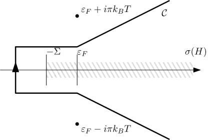
Figure 1. Contour $\mathcal{C}$ used to differentiate the potential-to-density mapping. Note that this differs from standard rectangular contours because we need to ensure that $(z-H)^{-1}$ remains Hilbert-Schmidt uniformly in $z\in\mathcal{C}$.

Step 2: $F_{\varepsilon_{F}}$ is analytic. Since potentials in $L^{2}_{\mathrm{per}}$ are infinitesimally $\Delta$-bounded, there is $\Sigma>0$ such that $\sigma(H)\subset[-\Sigma,+\infty)$ for all $W$ with $\|W\|_{L^{2}_{\mathrm{per}}}\leq R$. Let $\mathcal{C}$ be the contour given by Figure 1. This contour encloses the spectrum of $\sigma(H)$, avoids the poles of the Fermi-Dirac function at $\varepsilon_{F}+i\pi k_{B}T+2i\pi k_{B}T\mathbb{Z}$, and is asymptotic to $\operatorname*{Im}(z)=a\pm b\operatorname*{Re}(z)$ for large $z\in\mathcal{C}$, for some $a\in\mathbb{R},b>0$. The function $f_{\varepsilon_{F}}$ is therefore analytic inside $\mathcal{C}$, decays exponentially when $|z|\to\infty$, and we have

$$f_{\varepsilon_{F}}(H)=\frac{1}{2\pi i}\int_{\mathcal{C}}f_{\varepsilon_{F}}(z)(z-H)^{-1}dz$$

as bounded operators. Let $R_{z}=(z-H)^{-1}$. Because $d(z,\sigma(H))$ increases at the same rate as $\operatorname*{Re}(z)$, it follows from Lemma 3.6 that $B_{z}=R_{z}(1-\Delta)$ is bounded in operator norm, independently of $z\in\mathcal{C}$ (note that this would not be true for a rectangular contour). From the Kato-Seiler-Simon equality, there is therefore $C>0$ such that, for all $z\in\mathcal{C},\delta W\in L^{2}_{\mathrm{per}}$,

$$\|R_{z}\delta W\|_{{\mathfrak{S}}_{2,\mathrm{per}}}\leq\|B_{z}\|\|(1-\Delta)^{-1}\delta W\|_{{\mathfrak{S}}_{2,\mathrm{per}}}\leq C\|\delta W\|_{L^{2}_{\mathrm{per}}}.$$

Therefore, for $\|\delta W\|_{L^{2}_{\mathrm{per}}}\leq\frac{1}{2C}$, for all $z\in\mathcal{C}$, $(z-H-\delta W)$ is invertible, and

$$(z-H-\delta W)^{-1}=(1-R_{z}\delta W)^{-1}R_{z}=\sum_{n\geq 0}(R_{z}\delta W)^{n}R_{z}.$$

We can expand $f_{\varepsilon_{F}}(H+\delta W)$ as bounded operators:

$$f_{\varepsilon_{F}}(H+\delta W)-f_{\varepsilon_{F}}(H) =\frac{1}{2\pi i}\int_{\mathcal{C}}f_{\varepsilon_{F}}(z)\sum_{n\geq 1}(R_{z}\delta W)^{n}R_{z}dz.$$

For all $n\geq 1$, we have that

$$\left\|\left(R_{z}\delta W\right)^{n}R_{z}(1-\Delta)\right\|_{{\mathfrak{S}}_{2,\mathrm{per}}} \leq\|B_{z}\|\|R_{z}\delta W\|_{{\mathfrak{S}}_{2,\mathrm{per}}}^{n}\leq C^{n}\|\delta W\|_{L^{2}_{\mathrm{per}}}^{n}.$$

It follows from the decay properties of $f_{\varepsilon_{F}}$ on $\mathcal{C}$ that

$$\int_{\mathcal{C}}\sum_{n\geq 1}f_{\varepsilon_{F}}(z)\left\|\left(R_{z}\delta W\right)^{n}R_{z}(1-\Delta)\right\|_{{\mathfrak{S}}_{2,\mathrm{per}}}<\infty,$$

and therefore that $F_{\varepsilon_{F}}$ is analytic at $W$.

Step 3: $F_{\varepsilon_{F}}^{\prime}$ is self-adjoint and non-positive. From the previous computations, we have

$$F_{\varepsilon_{F}}^{\prime}(W)\cdot\delta W=\frac{1}{2\pi i}\int_{\mathcal{C}}f_{\varepsilon_{F}}(z)(R_{z}\delta WR_{z})(x,x)dz.$$

with $(R_{z}\delta WR_{z})(x,x)\in L^{2}_{\mathrm{per}}$ uniformly in $z\in\mathcal{C}$.

For all $z\in\mathcal{C}$, $R_{z}\delta WR_{z}$ is periodic with fibers $(z-H_{k})^{-1}\delta W(z-H_{k})^{-1}$. Inserting the spectral $(z-H_{k})^{-1}=\sum_{n\in\mathbb{N}}(z-\varepsilon_{nk})^{-1}|u_{nk}\rangle\langle u_{nk}|$, we get, for all $\delta W_{1},\delta W_{2}\in L^{2}_{\mathrm{per}}$,

$$\langle\delta W_{1},F_{\varepsilon_{F}}^{\prime}(W)\cdot\delta W_{2}\rangle$$

$$=\frac{1}{2\pi i}\int_{\mathcal{C}}f_{\varepsilon_{F}}(z)\fint_{\mathcal{B}}\sum_{n,m\in\mathbb{N}}\frac{1}{(z-\varepsilon_{nk})(z-\varepsilon_{mk})}\operatorname*{Tr}\Big{(}\overline{\delta W_{1}}|u_{nk}\rangle\langle u_{nk},\delta W_{2}u_{mk}\rangle\langle u_{mk}|\Big{)}dkdz.$$

$$=\frac{1}{2\pi i}\int_{\mathcal{C}}f_{\varepsilon_{F}}(z)\fint_{\mathcal{B}}\sum_{n,m\in\mathbb{N}}\frac{1}{(z-\varepsilon_{nk})(z-\varepsilon_{mk})}\langle\delta W_{1}u_{mk},u_{nk}\rangle\langle u_{nk},\delta W_{2}u_{mk}\rangle dkdz.$$

The absolute convergence of this sum in $L^{2}_{\mathrm{per}}$ follows from the estimates above. For completeness, we give a more direct proof. Let $e_{K}(x)=\frac{e^{iKx}}{\sqrt{|\Gamma|}}$. The $(e_{K})_{K\in\mathcal{R}^{*}}$ form a Hilbert basis of $L^{2}_{\mathrm{per}}$, and we have the property $\langle e_{K},\delta We_{K^{\prime}}\rangle=\frac{1}{\sqrt{|\Gamma|}}\langle e_{K-K^{\prime}},{\delta W}\rangle$ for all $\delta W\in L^{2},K,K^{\prime}\in\mathcal{R}^{*}$. It follows that

$$\sum_{n,m\in\mathbb{N}}\frac{|\langle u_{nk},\delta Wu_{mk}\rangle|^{2}}{|z-\varepsilon_{nk}|^{2}} =\sum_{n,m\in\mathbb{N},K,K^{\prime}\in\mathcal{R}^{*}}\frac{|\langle u_{nk},e_{K}\rangle\langle e_{K},\delta We_{K^{\prime}}\rangle\langle e_{K^{\prime}},u_{mk}\rangle|^{2}}{|z-\varepsilon_{nk}|^{2}}$$

$$=\frac{1}{|\Gamma|}\sum_{n\in\mathbb{N},K,K^{\prime}\in\mathcal{R}^{*}}\frac{|\langle u_{nk},e_{K}\rangle\langle e_{K-K^{\prime}},\delta W\rangle|^{2}}{|z-\varepsilon_{nk}|^{2}}$$

$$=\frac{\|\delta W\|_{L^{2}_{\mathrm{per}}}^{2}}{|\Gamma|}\sum_{n\in\mathbb{N},K\in\mathcal{R}^{*}}\frac{|\langle u_{nk},e_{K}\rangle|^{2}}{|z-\varepsilon_{nk}|^{2}}$$

$$=\frac{\|\delta W\|_{L^{2}_{\mathrm{per}}}^{2}}{|\Gamma|}\sum_{n\in\mathbb{N}}\frac{1}{|z-\varepsilon_{nk}|^{2}}$$

which is bounded uniformly in $k\in\mathcal{B},z\in\mathcal{C}$. The result follows by a Cauchy-Schwarz inequality. Performing the contour integration, we obtain the following sum-over-states formula

$$\langle\delta W_{1},F_{\varepsilon_{F}}^{\prime}(W)\cdot\delta W_{2}\rangle =\fint_{k\in\mathcal{B}}\sum_{n,m\in\mathbb{N}}\frac{f_{nk}-f_{mk}}{\varepsilon_{nk}-\varepsilon_{mk}}\langle\delta W_{1}u_{mk},u_{nk}\rangle\langle u_{nk},\delta W_{2}u_{mk}\rangle dk$$

where $f_{nk}=f_{\varepsilon_{F}}(\varepsilon_{nk})$, and with the convention that

$$\frac{f_{\varepsilon_{F}}(\varepsilon)-f_{\varepsilon_{F}}(\varepsilon)}{\varepsilon-\varepsilon}=f_{\varepsilon_{F}}^{\prime}(\varepsilon)$$

arising from the double pole $(z-\varepsilon_{mk})^{-2}$ when $\varepsilon_{nk}=\varepsilon_{mk}$. $F_{\varepsilon_{F}}^{\prime}(W)$ is therefore self-adjoint and, since

$$\langle\delta W,F_{\varepsilon_{F}}^{\prime}(W)\cdot\delta W\rangle =\fint_{k\in\mathcal{B}}\sum_{n,m\in\mathbb{N}}\frac{f_{nk}-f_{mk}}{\varepsilon_{nk}-\varepsilon_{mk}}\left|\langle u_{nk},\delta Wu_{mk}\rangle\right|^{2}dk$$

and $f_{\varepsilon_{F}}$ is decreasing, it follows that $F_{\varepsilon_{F}}^{\prime}(W)$ is non-positive.

Step 4: $F_{\varepsilon_{F}}^{\prime}(W)+\beta\Delta$ is negative. Assume that $F_{\varepsilon_{F}}^{\prime}(W)+\beta\Delta$ is not negative. This means that there exists a sequence $W_{n}$ of potentials with $\|W_{n}\|_{L^{2}_{\mathrm{per}}}=1$ such that

$$\langle W_{n},F_{\varepsilon_{F}}^{\prime}(W)\cdot W_{n}\rangle-\beta\int_{\Gamma}|\nabla W_{n}|^{2}\to 0.$$

Let $e\in L^{2}_{\mathrm{per}}$ be the constant function: $e(x)=1$. We have $\sum_{K\neq 0}|K|^{2}|c_{K}(W_{n})|^{2}\to 0$, so that $P_{e}^{\perp}W_{n}\to 0$ in $H^{1}$. Up to a subsequence, we can assume that $\langle e,W_{n}\rangle\to c$, with $c\in\mathbb{C}$. It follows from $W_{n}=P_{e}W_{n}+P_{e^{\perp}}W_{n}$ that $W_{n}\to ce$ in $L^{2}$, and that $|c|=\frac{1}{\sqrt{|\Gamma|}}$. Then,

$$\langle W_{n},F_{\varepsilon_{F}}^{\prime}(W)\cdot W_{n}\rangle \leq\fint_{k\in\mathcal{B}}f_{\varepsilon_{F}}^{\prime}(\varepsilon_{1k})|\langle u_{1k},W_{n}u_{1k}\rangle|^{2}dk$$

$$\to\frac{1}{\sqrt{|\Gamma|}}\fint_{k\in\mathcal{B}}f_{\varepsilon_{F}}^{\prime}(\varepsilon_{1k})dk<0.$$

where we have used that $\||u_{1k}|^{2}\|_{L^{2}_{\mathrm{per}}}\leq C\|u_{1k}\|_{H^{1}_{\mathrm{per}}}^{2}$ is bounded uniformly in $k$. ∎

4.1. Self-consistent Fermi level

We now solve the equation $\int_{\Gamma}F_{\varepsilon_{F}}(W)=N_{\rm el}$ for $\varepsilon_{F}$.

Lemma 4.2.

For all $W\in L^{2}_{\mathrm{per}}$ and $N_{\rm el}>0$, the equation $\int_{\Gamma}F_{\varepsilon_{F}}(W)=N_{\rm el}$ has a unique solution $\varepsilon_{F}(W)$. The map

$$F(W) =F_{\varepsilon_{F}(W)}(W)$$

is analytic from $L^{2}_{\mathrm{per}}$ to $L^{2}_{\mathrm{per}}$. Its differential $F^{\prime}(W)$ is self-adjoint and non-positive, and satisfies $F^{\prime}(W)\cdot e=0$ where $e$ is the constant function.

Proof.

Let

$$\mathcal{N}(\varepsilon_{F},W)=\langle e,F_{\varepsilon_{F}}(W)\rangle=\fint_{\mathcal{B}}\sum_{n\in\mathbb{N}}f_{\varepsilon_{F}}(\varepsilon_{nk})dk$$

be the total number of electrons with Fermi level $\varepsilon_{F}$. Then by the previous lemma $\mathcal{N}$ is analytic on $\mathbb{R}\times L^{2}_{\mathrm{per}}$, with

$$\frac{\partial\mathcal{N}}{\partial\varepsilon_{F}}(\varepsilon_{F},W) =-\langle e,F_{\varepsilon_{F}}^{\prime}(W)\cdot e\rangle=-\fint_{\mathcal{B}}\sum_{n\in\mathbb{N}}f^{\prime}_{\varepsilon_{F}}(\varepsilon_{nk})dk>0$$

$$\frac{\partial\mathcal{N}}{\partial W}(\varepsilon_{F},W)\cdot\delta W =\langle e,F_{\varepsilon_{F}}^{\prime}(W)\cdot\delta W\rangle=\langle F_{\varepsilon_{F}}^{\prime}(W)\cdot e,\delta W\rangle$$

For all $W\in L^{2}_{\mathrm{per}}$, $\mathcal{N}(\cdot,W)$ has limit $0$ at $-\infty$ and $+\infty$ at $+\infty$, so that there is a unique solution $\varepsilon_{F}(W)$ of $\mathcal{N}(\varepsilon_{F},W)=N_{\rm el}$. From the implicit function theorem, we get that $\varepsilon_{F}(W)$ is analytic on $L^{2}_{\mathrm{per}}$ and

$$\varepsilon_{F}^{\prime}(W)\cdot\delta W=\frac{1}{\langle e,F_{\varepsilon_{F}}^{\prime}(W)\cdot e\rangle}\langle F_{\varepsilon_{F}}^{\prime}(W)\cdot e,\delta W\rangle$$

and therefore

$$F^{\prime}(W)\cdot\delta W =F^{\prime}_{\varepsilon_{F}}(W)\cdot\delta W-\frac{1}{\langle e,F_{\varepsilon_{F}}^{\prime}(W)\cdot e\rangle}\langle F_{\varepsilon_{F}}^{\prime}(W)\cdot e,\delta W\rangle\;F_{\varepsilon_{F}}^{\prime}(W)\cdot e$$

In particular, $F^{\prime}(W)\cdot e=0$ and $F^{\prime}(W)$ is self-adjoint.

The expression above is of the form $F^{\prime}(W)=A-\frac{1}{\langle e,Ae\rangle}|Ae\rangle\langle Ae|$, with $A=F_{\varepsilon_{F}}^{\prime}(W)$ bounded, self-adjoint and non-positive on a Hilbert space $\mathcal{H}$ and $e\in\mathcal{H}$. In particular, $F^{\prime}(W)$ is self-adjoint, $F^{\prime}(W)\cdot e=0$, and we compute, for all $x\in\mathcal{H}$,

$$\left\langle x,\left(A-\frac{1}{\langle e,Ae\rangle}|Ae\rangle\langle Ae|\right)x\right\rangle =-\left(\||A|^{1/2}x\|^{2}-\frac{|\langle|A|^{1/2}x,|A|^{1/2}e\rangle|^{2}}{\||A|^{1/2}e\|^{2}}\right)\leq 0$$

by the Cauchy-Schwartz inequality, from where it follows that $F^{\prime}(W)$ is non-positive.

∎

We now look for solutions $W\in L^{2}_{\mathrm{per}}$ of the equation

$$W=W_{\mathrm{nucl}}+{v_{\mathrm{per}}}F(W).$$

We are ready for the

Proof of Theorem 1.1..

Set

$$M_{\alpha}(W,W_{\mathrm{nucl}})=W+\alpha(W_{\mathrm{nucl}}+{v_{\mathrm{per}}}F(W)-W)$$

In particular, $M_{\alpha}$ is analytic from $L^{2}_{\mathrm{per}}$ to itself. From Theorem 3.3, we only need to check that the spectral radius of the operator

$$J_{\alpha}=1+\alpha({v_{\mathrm{per}}}F^{\prime}(W^{*})-1)$$

is smaller than $1$ for $\alpha$ small enough. This is ensured by the fact that ${v_{\mathrm{per}}}$ and $F^{\prime}(W^{*})$ are bounded operators on $L^{2}_{\mathrm{per}}$ and ${v_{\mathrm{per}}}$ is non-negative, so that, from Lemma 3.1,

$$\sigma({v_{\mathrm{per}}}F^{\prime}(W^{*}))\setminus\{0\}=\sigma(\sqrt{v_{\mathrm{per}}}F^{\prime}(W^{*})\sqrt{v_{\mathrm{per}}})\setminus\{0\}$$

This last operator is a non-positive self-adjoint bounded operator on $L^{2}_{\mathrm{per}}$, hence the result. ∎

5. The defect problem

In this section we fix $W_{\mathrm{per}}\in L^{2}_{\mathrm{per}}$ and $\varepsilon_{F}\in\mathbb{R}$. Let

$$H_{\mathrm{per}}=-\Delta+W_{\mathrm{per}}$$

be the background periodic Hamiltonian.

We first investigate the renormalized potential-to-density mapping.

Lemma 5.1.

There is a neighborhood $\mathcal{V}$ of $0$ in $L^{2}$ in which the map

$$G(V)=(f_{\varepsilon_{F}}(H_{\mathrm{per}}+V)-f_{\varepsilon_{F}}(H_{\mathrm{per}}))(x,x)$$

is analytic from $L^{2}_{N}$ to $L^{2}_{N}$ for all $N\geq 0$.

Let $\chi_{0}=G^{\prime}(0)$. Then $V\mapsto G(V)-\chi_{0}V$ maps $\mathcal{V}\cap L^{2}_{N}$ to $L^{2}_{2N}$ for all $N\geq 0$.

Proof.

Step 1: the case $N=0$. The proof of this step is similar to that of Lemma 4.1. We take a contour $\mathcal{C}$ enclosing the spectrum of $H_{\mathrm{per}}$ with the same shape as in Figure 1, which encloses the spectrum of $H_{\mathrm{per}}+V$ for $\|V\|_{L^{2}}$ small because $L^{2}$ potentials are infinitesimally $\Delta$-bounded. From Lemma 3.6, there is $C>0$ such that, for all $z\in\mathcal{C}$ and $V\in L^{2}$,

$$\|R_{z}V\|_{{\mathfrak{S}}_{2}}=\|R_{z}(1-\Delta)(1-\Delta)^{-1}V\|_{{\mathfrak{S}}_{2}}\leq C\|V\|_{L^{2}}.$$

with $R_{z}=(z-H_{\mathrm{per}})^{-1}$. It follows that, for $\|V\|_{L^{2}}\leq\frac{1}{2C}$, $(1-R_{z}V)$ is invertible, and we have

$$f_{\varepsilon_{F}}(H_{\mathrm{per}}+V)-f_{\varepsilon_{F}}(H_{\mathrm{per}}) =\frac{1}{2\pi i}\int_{\mathcal{C}}f_{\varepsilon_{F}}(z)\left(\left(z-(H_{\mathrm{per}}+V)\right)^{-1}-(z-H_{\mathrm{per}})^{-1}\right)dz$$

(13) $$=\frac{1}{2\pi i}\int_{\mathcal{C}}f_{\varepsilon_{F}}(z)\sum_{n\geq 1}(R_{z}V)^{n}R_{z}dz$$

as bounded operators. From the estimate

$$\|(R_{z}V)^{n-1}R_{z}VR_{z}(1-\Delta)\|_{{\mathfrak{S}}_{2}}\leq\|R_{z}(1-\Delta)\|\|R_{z}V\|_{{\mathfrak{S}}_{2}}^{n}\leq C^{n}\|V\|_{L^{2}}^{n}$$

with $C$ uniform in $z\in\mathcal{C}$ and the decay properties of $f_{\varepsilon_{F}}$, it follows that the expansion (13) converges absolutely. Therefore, $f_{\varepsilon_{F}}(H_{\mathrm{per}}+V)-f_{\varepsilon_{F}}(H_{\mathrm{per}})$ can be associated a density $G(V)\in L^{2}$, and $G$ is analytic in a neighborhood of $0$.

Step 2: Bloch structure of the expansion of the density at all orders. We first note that

$$H_{k+q}-H_{k}=2(-i\nabla+k)\cdot q+|q|^{2}.$$

The bounded operator $R_{z}=(z-H)^{-1}$ on $L^{2}$ is periodic with fibers $R_{z,k}=(z-H_{k})^{-1}$. Since $R_{z,k}(1-\Delta)$ is bounded uniformly in $z\in\mathcal{C}$ and $k\in\mathcal{B}$,

$$\|R_{z,k}(2(-i\nabla+k)\cdot q+|q|^{2})\|=\|R_{z,k}(1-\Delta)(1-\Delta)^{-1}(2(-i\nabla+k)\cdot q+|q|^{2})\|\leq C(|q|+|q|^{2}).$$

For $q$ small enough, we then have

$$R_{z,k+q}=\sum_{n\geq 0}\Big{(}R_{z,k}(2(-i\nabla+k)\cdot q+|q|^{2})\Big{)}^{n}R_{z,k}$$

and, from the previous estimate, $R_{z,k}$ is analytic in the $\|\cdot(1-\Delta)\|_{{\mathfrak{S}}_{2,\mathrm{per}}}$ topology, uniformly in $z\in\mathcal{C}$ and $k\in\mathcal{B}$.

For $z\in\mathcal{C}$, let

$$D^{(n)}_{z}(V)=((R_{z}V)^{n}R_{z})(x,x).$$

We first consider the first-order term $D^{(1)}_{z}$. Let $V=\int_{\mathcal{B}}e^{iqx}V_{q}(x)dq\in L^{2}$. Elementary computations show that if $A$ is a periodic operator with fibers $A_{k}$, then $e^{-iqx}Ae^{iqx}$ is a periodic operator with fibers $A_{k+q}$, and that $e^{iqx}A$ has density

$$(e^{iqx}A)(x,x)=e^{iqx}A(x,x)=e^{iqx}\fint_{\mathcal{B}}A_{k}(x,x)dk.$$

Therefore,

$$D_{z}^{(1)}(V) =\int_{\mathcal{B}}(e^{iqx}e^{-iqx}R_{z}e^{iqx}V_{q}R_{z})(x,x)dq=\int_{\mathcal{B}}e^{iqx}\fint_{\mathcal{B}}(R_{z,k+q}V_{q}R_{z,k})(x,x)dk\,dq$$

$$D_{z}^{(1)}(V)_{q} =\fint_{\mathcal{B}}(R_{z,k+q}V_{q}R_{z,k})(x,x)dk.$$

Similarly, in the general case,

(14) $$D_{z}^{(n)}(V)_{q}=\int_{q_{1},\dots,q_{n-1}\in\mathcal{B}}\fint_{k\in\mathcal{B}}(R_{z,k+q}V_{q-q_{1}}R_{z,k+q_{1}}V_{q_{1}-q_{2}}\cdots R_{z,k})(x,x)dk\,dq_{1}\cdots dq_{n-1}$$

Step 3: the case $N>0$. Since for $i=1,2,3$

(15) $$(x_{i}D^{(n)}_{z}(V))_{q} =i\partial_{q_{i}}D^{(n)}_{z}(V)_{q}$$

and $R_{z,k}$ is analytic for the $\|\cdot(1-\Delta)\|_{{\mathfrak{S}}_{2,\mathrm{per}}}$ topology, uniformly in $z\in\mathcal{C},k\in\mathcal{B}$, the repeated application of (15) to (14) yields a bound of the form

$$\|D^{(n)}_{z}(V)\|_{L^{2}_{N}}\leq C_{N}\|V\|_{L^{2}_{N}}C^{n-1}\|V\|_{L^{2}}^{n-1}$$

for all $N\geq 0$, with $C$ independent on $N$, this bound being uniform in $z\in\mathcal{C}$.

It follows that, for $\|V\|_{L^{2}}\leq\frac{1}{2C}$, for all $N$, we have the absolutely convergent expansion

$$G(V) =\frac{1}{2\pi i}\int_{\mathcal{C}}f_{\varepsilon_{F}}(z)\sum_{n\geq 1}D^{(n)}_{z}(V)dz$$

in $L^{2}_{N}$.

Step 4: $G(V)-\chi_{0}V:L^{2}_{N}\mapsto L^{2}_{2N}$. We have

$$G(V)-\chi_{0}V =\frac{1}{2\pi i}\int_{\mathcal{C}}f_{\varepsilon_{F}}(z)\sum_{n\geq 2}D^{(n)}_{z}(V)dz.$$

Consider terms of the form

(16) $$I(q)= \int_{q_{1},\dots,q_{n-1}\in\mathcal{B}}\fint_{k\in\mathcal{B}}(R_{z,k+q}^{(1)}V^{(1)}_{q-q_{1}}R_{z,k+q_{1}}^{(2)}V^{(2)}_{q_{1}-q_{2}}R_{z,k+q_{2}}V_{q_{2}-q_{3}}\cdots R_{z,k})(x,x)dkdq_{1}\cdots dq_{n-1}$$

where $R^{(1)}_{z,k},R^{(2)}_{z,k}$ are $R_{z,k}$ or their derivatives, and $V^{(1)}_{q},V^{(2)}_{q}$ are $V_{q}$ or its derivatives. Performing the change of variable $q_{1}^{\prime}=q-q_{1}$, we obtain

$$I(q) =-\int_{q_{1}^{\prime}\in q-\mathcal{B}}\int_{q_{2},\dots,q_{n-1}\in\mathcal{B}}\fint_{k\in\mathcal{B}}(R_{z,k+q}^{(1)}V^{(1)}_{q_{1}^{\prime}}R_{z,k+q-q_{1}^{\prime}}^{(2)}V^{(2)}_{q-q_{1}^{\prime}-q_{2}}R_{z,k+q_{2}}V_{q_{2}-q_{3}}\cdots R_{z,k})(x,x)dkdq_{1}^{\prime}\cdots dq_{n-1}$$

$$=-\int_{q_{1}^{\prime},\dots,q_{n-1}\in\mathcal{B}}\fint_{k\in\mathcal{B}}(R_{z,k+q}^{(1)}V^{(1)}_{q_{1}^{\prime}}R_{z,k+q-q_{1}^{\prime}}^{(2)}V^{(2)}_{q-q_{1}^{\prime}-q_{2}}R_{z,k+q_{2}}V_{q_{2}-q_{3}}\cdots R_{z,k})(x,x)dkdq_{1}^{\prime}\cdots dq_{n-1},$$

where the quasi-periodicity of the Bloch transform implies that $q_{1}^{\prime}\mapsto V^{(1)}_{q_{1}^{\prime}}R_{z,k+q-q_{1}^{\prime}}^{(2)}V^{(2)}_{q-q_{1}^{\prime}-q_{2}}$ is $\mathcal{R}^{*}$-periodic, and therefore that we can integrate $q_{1}^{\prime}$ over $\mathcal{B}$ rather than $q-\mathcal{B}$. This shows that we can transfer the $q$ dependence from $V^{(1)}$ to $V^{(2)}$ in the convolution-like terms of the form (16).

Let $p_{2N}$ be a polynomial of degree $2N$. Applying (15) successively to $p_{2N}(x)D_{z}^{(n)}(V)$ and using the above procedure to the divide the $2N$ derivatives between $V^{(1)}_{q}$ and $V^{(2)}_{q}$, we obtain that $(p_{2N}(x)D_{z}^{(n)}(V))_{q}$ contains terms of the form (16) with $V^{(1)}_{q}$ and $V^{(2)}_{q}$ being derivatives of $V_{q}$ of order at most $N$. Using the analyticity of $k\mapsto R_{z,k}$, we obtain a bound of the form

$$\|D^{(n)}_{z}(V)\|_{L^{2}_{2N}}\leq C_{N}\|V\|_{L^{2}_{N}}^{2}C^{n-2}\|V\|_{L^{2}}^{n-2}$$

where $C$ is independent of $N$, the bound being uniform in $z\in\mathcal{C}$. The result follows.

∎

Recall that the operator ${v_{\rm c}}$ is given by the convolution

$$({v_{\rm c}}\rho)(x)=\frac{1}{4\pi}\int_{\mathbb{R}^{3}}\frac{\rho(y)}{|x-y|}dy.$$

In Fourier space, this is a multiplication by $\frac{1}{|q|^{2}}$. This is an unbounded non-negative self-adjoint operator on $L^{2}$. We denote its formal inverse by ${v_{\rm c}}^{-1}=-\Delta$, also an unbounded non-negative self-adjoint operator on $L^{2}$. ${v_{\rm c}}^{-1}$ does not have a spectral gap at zero, but $-\chi_{0}+{v_{\rm c}}^{-1}$ does:

Lemma 5.2.

Let $N\geq 0$. The operator $-\chi_{0}+{v_{\rm c}}^{-1}$ is self-adjoint and positive on $L^{2}$, and its inverse is bounded from $H^{-2}_{N}$ to $L^{2}_{N}$.The operator $\varepsilon=1-{v_{\rm c}}\chi_{0}$ is invertible in $L^{2}_{N}$, with bounded inverse

$$\varepsilon^{-1}=(1-{v_{\rm c}}\chi_{0})^{-1}=\left(-\chi_{0}+{v_{\rm c}}^{-1}\right)^{-1}{v_{\rm c}}^{-1}.$$

The operator $\mathcal{K}\varepsilon$ is therefore bounded and invertible on $L^{2}_{N}$.

Proof.

We have, for $V\in L^{2}$ with Bloch transform $V_{q}$

$$\chi_{0}V =\frac{1}{2\pi i}\int_{\mathcal{C}}f_{\varepsilon_{F}}(z)\int_{\mathcal{B}}\fint_{\mathcal{B}}(R_{z,k+q}V_{q}R_{z,k})(x,x)dkdqdz$$

and therefore $\chi_{0}$ is fibered, with fibers

(17) $$\chi_{0,q}W =\frac{1}{2\pi i}\int_{\mathcal{C}}f_{\varepsilon_{F}}(z)\fint_{\mathcal{B}}(R_{z,k+q}WR_{z,k})(x,x)dkdz$$

for $W\in L^{2}_{\mathrm{per}}$. As in Lemma 4.1, inserting the decomposition $R_{z,k}=\sum_{n\in\mathbb{N}}(z-\varepsilon_{nk})^{-1}|u_{nk}\rangle\langle u_{nk}|$, we obtain the sum-over-states formula

$$\langle W_{1},\chi_{0,q}W_{2}\rangle =\fint_{\mathcal{B}}\sum_{n,m\geq 0}\frac{f_{n,k+q}-f_{m,k}}{\varepsilon_{n,k+q}-\varepsilon_{m,k}}\langle W_{1}u_{m,k},u_{nk+q}\rangle\langle u_{nk+q},W_{2}u_{m,k}\rangle dk$$

converging absolutely, from where it follows that $\chi_{0,q}$ is self-adjoint and non-positive on $L^{2}$ for all $q$, and therefore that $\chi_{0}$ is too.

It follows from the regularity of $R_{z,k}$ and (17) that $\chi_{0,k}$ is analytic as bounded operators in $L^{2}_{\mathrm{per}}$, with $\chi_{0,0}=F_{\varepsilon_{F}}^{\prime}(W_{\mathrm{per}})$. The operator ${v_{\rm c}}^{-1}=-\Delta$ has fibers ${v_{\rm c,k}}^{-1}=(-i\nabla+k)^{2}$ positive except at $k=0$. Using Lemma 4.1 with $\beta=1/2$, it follows that

$$-\chi_{0,k}+\frac{1}{2}{v_{\rm c,k}}^{-1}=-(\chi_{0,k}-F_{\varepsilon_{F}}^{\prime}(W_{\mathrm{per}}))-F_{\varepsilon_{F}}^{\prime}(W_{\mathrm{per}})+\frac{1}{2}{v_{\rm c,k}}^{-1}$$

is bounded away from zero for $k$ small, and therefore for all $k$. Therefore, there is $c>0$ such that

$$-\chi_{0}+{v_{\rm c}}^{-1}=-\chi_{0}+\frac{1}{2}{v_{\rm c}}^{-1}+\frac{1}{2}{v_{\rm c}}^{-1}\geq c(1-\Delta)$$

as quadratic forms, from where it follows that $(-\chi_{0}+{v_{\rm c}}^{-1})^{-1}\leq\frac{1}{c}(1-\Delta)^{-1}$ as quadratic forms and then that, for all $V\in L^{2}$, $\|(-\chi_{0}+{v_{\rm c}}^{-1})^{-1}V\|_{L^{2}}\leq\frac{1}{c}\|(1-\Delta)^{-1}V\|_{L^{2}}$. The operator $(-\chi_{0}+{v_{\rm c}}^{-1})^{-1}$ is therefore bounded from $H^{-2}$ to $L^{2}$.

Its fibers are $(\chi_{0,k}+{v_{\rm c,k}}^{-1})^{-1}$ and, for $q$ small enough,

$$(\chi_{0,k+q}+{v_{\rm c,k}}^{-1})^{-1}=\sum_{n\geq 0}\Big{(}(\chi_{0,k}+{v_{\rm c,k}}^{-1})^{-1}(\chi_{0,k+q}-\chi_{0,k})^{n}\Big{)}(\chi_{0,k}+{v_{\rm c,k}}^{-1})^{-1}$$

which shows that the family $(\chi_{0}+{v_{\rm c}}^{-1})^{-1}_{k}$ is analytic on $\mathcal{B}$ as operators from $H^{-2}_{\mathrm{per}}$ to $L^{2}_{\mathrm{per}}$, and therefore that $(\chi_{0}+{v_{\rm c}}^{-1})^{-1}$ is bounded from $H^{-2}_{N}$ to $L^{2}_{N}$. It then follows that $\varepsilon$ is invertible on $L^{2}_{N}$, with inverse

$$\varepsilon^{-1}=(1-{v_{\rm c}}\chi_{0})^{-1}=\left(-\chi_{0}+{v_{\rm c}}^{-1}\right)^{-1}{v_{\rm c}}^{-1}.$$

Finally, we have

$$(\mathcal{K}\varepsilon)^{-1}=(-\chi_{0}+{v_{\rm c}}^{-1})^{-1}{v_{\rm c}}^{-1}\mathcal{K}^{-1}=(-\chi_{0}+{v_{\rm c}}^{-1})^{-1}(1-\Delta),$$

hence the result. ∎

We are now ready for the

Proof of Theorem 1.2..

We proceed as in Theorem 1.1, and apply Theorem 3.3 to

$$M(V,V_{\mathrm{def}})=V+\alpha\mathcal{K}(V_{\mathrm{def}}+{v_{\rm c}}G(V)-V),$$

analytic in a neighborhood of $0$ in $L^{2}\times{v_{\rm c}}H^{-2}$ to $L^{2}$, with Jacobian at $(0,0)$

$$J_{\alpha}=1-\alpha\mathcal{K}+\alpha\mathcal{K}{v_{\rm c}}\chi_{0}=1-\alpha\mathcal{K}\varepsilon.$$

Since ${\mathcal{K}{v_{\rm c}}}=(1-\Delta)^{-1}$ is bounded, self-adjoint and non-negative on $L^{2}$, we have

$$\sigma(\mathcal{K}{v_{\rm c}}\chi_{0})\setminus\{0\}=\sigma(\sqrt{\mathcal{K}{v_{\rm c}}}\chi_{0}\sqrt{\mathcal{K}{v_{\rm c}}})\setminus\{0\}.$$

It follows that by taking $\alpha_{0}$ small enough, we can impose that $\sigma(J_{\alpha})\subset(-1,1]$. Since from Lemma 5.2 the operator $\mathcal{K}\varepsilon$ is invertible on $L^{2}$, we even have that $\sigma(J_{\alpha})\subset(-1,1)$, hence the result. ∎

Proof of Theorem 1.3..

The proof is based on a bootstrap argument on the equation

(18) $$V=\varepsilon^{-1}(V_{\mathrm{def}}+{v_{\rm c}}(G(V)-\chi_{0}V))$$

satisfied by $V(V_{\mathrm{def}})$.

For the base case $N=1$, we prove that $V(V_{\mathrm{def}})\in L^{2}_{1}$ by applying Theorem 3.3 to

$$M(V,V_{\mathrm{def}})=\varepsilon^{-1}(V_{\mathrm{def}}+{v_{\rm c}}(G(V)-\chi_{0}V)),$$

an analytic map from $L^{2}_{1}\times{v_{\rm c}}H^{-2}_{1}$ to $L^{2}_{1}$ with Jacobian $0$ at $(0,0)$. It follows from the uniqueness of $V(V_{\mathrm{per}})$ that $V(V_{\mathrm{per}})\in L^{2}_{1}$.

We then use the fact that $M(\cdot,V_{\mathrm{def}})$ maps $L^{2}_{1}$ to $L^{2}_{2}$ to conclude from (18) that $V(V_{\mathrm{per}})\in L^{2}_{2}$. Repeating this argument, we obtain that $V(V_{\mathrm{per}})\in L^{2}_{N}$. ∎

References

- [1] S.L. Adler. Quantum theory of the dielectric constant in real solids. Physical Review, 126(2):413, 1962.
- [2] M. Benzi, P. Boito, and N. Razouk. Decay properties of spectral projectors with applications to electronic structure. SIAM review, 55(1):3–64, 2013.
- [3] É. Cancès, A. Deleurence, and M. Lewin. A new approach to the modeling of local defects in crystals: The reduced Hartree-Fock case. Communications in Mathematical Physics, 281(1):129–177, 2008.
- [4] É Cancès and V. Ehrlacher. Local defects are always neutral in the Thomas–Fermi–von Weiszäcker theory of crystals. Archive for rational mechanics and analysis, 202(3):933–973, 2011.
- [5] É Cancès, V. Ehrlacher, D. Gontier, A. Levitt, and D. Lombardi. Numerical quadrature in the Brillouin zone for periodic Schrodinger operators. arXiv preprint arXiv:1805.07144, 2018.
- [6] É Cancès and C. Le Bris. On the convergence of SCF algorithms for the Hartree-Fock equations. ESAIM: Mathematical Modelling and Numerical Analysis, 34(4):749–774, 2000.
- [7] É. Cancès and M. Lewin. The dielectric permittivity of crystals in the reduced Hartree–Fock approximation. Archive for Rational Mechanics and Analysis, 197(1):139–177, 2010.
- [8] É Cancès and G. Stoltz. A mathematical formulation of the random phase approximation for crystals. Annales de l’Institut Henri Poincare (C) Non Linear Analysis, 29(6):887–925, 2012.
- [9] Eric Cancès, Gaspard Kemlin, and Antoine Levitt. Convergence analysis of direct minimization and self-consistent iterations. arXiv preprint arXiv:2004.09088, 2020.
- [10] I. Catto, C. Le Bris, and P-L Lions. On the thermodynamic limit for Hartree–Fock type models. Annales de l’Institut Henri Poincaré (C) Non Linear Analysis, 18(6):687–760, 2001.
- [11] H. Chen, J. Lu, and C. Ortner. Thermodynamic limit of crystal defects with finite temperature tight binding. Archive for Rational Mechanics and Analysis, 230(2):701–733, 2018.
- [12] R. Frank, M. Lewin, E. Lieb, and R. Seiringer. A positive density analogue of the Lieb–Thirring inequality. Duke Mathematical Journal, 162(3):435–495, 2013.
- [13] D. Gontier and S. Lahbabi. Supercell calculations in the reduced Hartree–Fock model for crystals with local defects. Applied Mathematics Research eXpress, 2017(1):1–64, 2016.
- [14] R.B. Holmes. A formula for the spectral radius of an operator. The American Mathematical Monthly, 75(2):163–166, 1968.
- [15] G.P. Kerker. Efficient iteration scheme for self-consistent pseudopotential calculations. Physical Review B, 23(6):3082, 1981.
- [16] A. Lechleiter. The Floquet–Bloch transform and scattering from locally perturbed periodic surfaces. Journal of Mathematical Analysis and Applications, 446(1):605–627, 2017.
- [17] A. Levitt. Convergence of gradient-based algorithms for the Hartree-Fock equations. ESAIM: Mathematical Modelling and Numerical Analysis, 46(6):1321–1336, 2012.
- [18] E. Lieb and B. Simon. The Thomas-Fermi theory of atoms, molecules and solids. Advances in Mathematics, 23(1):22–116, 1977.
- [19] F. Nazar and C. Ortner. Locality of the Thomas–Fermi–von Weizsäcker Equations. Archive for Rational Mechanics and Analysis, 224(3):817–870, 2017.
- [20] F. Nier. A variational formulation of Schrödinger-Poisson systems in dimension d 3. Communications in partial differential equations, 18(7-8):1125–1147, 1993.
- [21] E. Prodan, S.R. Garcia, and M. Putinar. Norm estimates of complex symmetric operators applied to quantum systems. Journal of Physics A: Mathematical and General, 39(2):389, 2005.
- [22] M. Reed and B. Simon. Analysis of operators, vol. IV of Methods of modern mathematical physics, 1978.
- [23] Y. Saad. Iterative methods for sparse linear systems, volume 82. SIAM, 2003.
- [24] B. Simon. Trace ideals and their applications. American Mathematical Soc., 2010.
- [25] J-P Solovej. Proof of the ionization conjecture in a reduced Hartree-Fock model. Inventiones mathematicae, 104(1):291–311, 1991.
- [26] H. Walker and P. Ni. Anderson acceleration for fixed-point iterations. SIAM Journal on Numerical Analysis, 49(4):1715–1735, 2011.
- [27] N. Wiser. Dielectric constant with local field effects included. Physical Review, 129(1):62, 1963.