A Survey on Periocular Biometrics Research

Abstract

Periocular refers to the facial region in the vicinity of the eye, including eyelids, lashes and eyebrows. While face and irises have been extensively studied, the periocular region has emerged as a promising trait for unconstrained biometrics, following demands for increased robustness of face or iris systems. With a surprisingly high discrimination ability, this region can be easily obtained with existing setups for face and iris, and the requirement of user cooperation can be relaxed, thus facilitating the interaction with biometric systems. It is also available over a wide range of distances even when the iris texture cannot be reliably obtained (low resolution) or under partial face occlusion (close distances). Here, we review the state of the art in periocular biometrics research. A number of aspects are described, including: $i$) existing databases, $ii$) algorithms for periocular detection and/or segmentation, $iii$) features employed for recognition, $iv$) identification of the most discriminative regions of the periocular area, $v$) comparison with iris and face modalities, $vi$) soft-biometrics (gender/ethnicity classification), and $vii$) impact of gender transformation and plastic surgery on the recognition accuracy. This work is expected to provide an insight of the most relevant issues in periocular biometrics, giving a comprehensive coverage of the existing literature and current state of the art.

1 Introduction

Periocular biometrics has been shown as one of the most discriminative regions of the face, gaining attention as an independent method for recognition or a complement to face and iris modalities under non-ideal conditions (Santos and Proenca, 2013; Nigam et al., 2015). The typical elements of the periocular region are labeled in Figure 1, left. This region can be acquired largely relaxing the acquisition conditions, in contraposition to the more carefully controlled conditions usually needed in face or iris modalities, making it suitable for unconstrained and uncooperative scenarios. Another advantage is that the problem of iris segmentation is automatically avoided, which can be an issue in difficult images (Jillela et al., 2013).

This paper presents a survey of periocular research works found in the literature. We provide a comprehensive framework covering different aspects, from existing databases (Section 2), to algorithms for detection of the periocular region (Section 3), and features for recognition (Section 4). Databases utilized include face and iris databases (since the periocular area appears in such data), as well as newer databases capturing specifically the periocular area. Although initial studies have made use of annotated data, detection and segmentation of the periocular region has become a research target in itself. We also provide a taxonomy of the features employed for periocular recognition, which can be divided between those performing a global analysis of the image (extracting properties describing an entire ROI) and those performing local analysis (extracting properties of the neighborhood of a set of sparse selected key points).

Most recognition algorithms work by applying feature extraction and/or key points detection to a predefined ROI around the eye (Figure 1, right). This holistic approach implies that some components not relevant for identity recognition, such as hair or glasses, might be erroneously taken into account (Proenca et al., 2014). It can also be the case that a certain feature is not equally discriminative in all parts of the periocular region. Some works have addressed these problems, as presented in Section 5. Since the periocular area appears in face and iris images, comparison and fusion with these modalities has been also proposed, which is the focus of Section 6. Besides personal recognition, a number of other tasks have been also proposed using features extracted from the periocular region. In this direction, Section 7 deals with issues like soft-biometrics (gender/ethnicity classification), and impact of gender transformation and plastic surgery on the recognition accuracy. We finally conclude the paper by highlighting current trends and future directions in periocular biometrics.

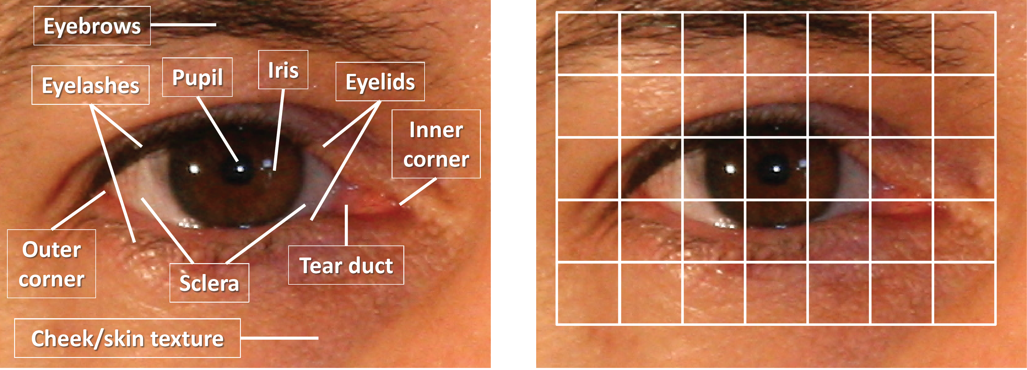
Fig. 1: Left: elements of the periocular region. Right: region of interest around the eye for feature extraction. Image from UBIRIS v2 database.

2 Databases

Table 1 summarizes the databases used in periocular research. Some sample images are shown in Figure 2. Very few databases have been designed specifically for periocular research, with face and iris databases mostly used for this purpose. The ‘best accuracy’ shown in Table 1 should be taken as an approximate indication only, since different works may employ different subsets of the database or a different protocol. A general tendency, however, is that facial databases exhibit a better accuracy. These are the most used databases, so each new work builds on top of previous research, resulting in additional improvements. The accuracy with newer periocular databases are only some steps behind, demonstrating the capabilities of the periocular modality even in difficult scenarios, where new research leaps are expected to bring accuracy to even better levels. The following is a short description of each database, highlighting the features not contained in Table 1.

Table 1: Databases used in periocular research. Only public available databases are included. The ‘best accuracy’ indicates the best performance reported in the literature (Table 3). The availability of ground-truth information is also indicated, either provided with the database, or available elsewhere.

								Variability factors						Best accuracy
Name	Reference	Subjects	Sessions	Data	Size	Ground-truth	Illumination	Cross-spectrum	Distance	Expression	Lightning	Occlusion	Pose	EER	Rank-1
FACIAL DATABASES
M2VTS	(Pigeon and Vandendorpe, 1997)	37	5	185 videos	286$\times$350		VW	no	no	yes	no	yes	yes	0.3%	n/a
AR	(Martinez and Benavente, 1998)	126	2	$>$4000 images	768$\times$576	yes	VW	no	no	yes	yes	yes	no	n/a	76%
GTDB	(Georgia Tech face database (), GTDB)	50	2-3	750 images	640$\times$480	yes	VW	no	yes	yes	yes	no	yes	0.25%	89.2%
Caltech	(Caltech face database, )	27	n/a	450 images	896$\times$592	yes	VW	no	no	yes	yes	no	no	0.12%	n/a
FERET	(Phillips et al., 2000)	1199	15	14126 images	512$\times$768	yes	VW	no	no	yes	yes	no	yes	0.22%	96.8%
CMU-H	(Denes et al., 2002)	54	1-5	764 videos	640$\times$480		450-1100nm	yes	no	no	yes	no	no	n/a	97.2%
FRGC	(Phillips et al., 2005)	741	1	36818 images	$\sim$1200$\times$1400	yes	VW	no	yes	yes	yes	no	no	0.09%	98.3%
MORPH	(Ricanek and Tesafaye, 2006)	515	2-5	1690 images	400$\times$500	yes	VW	no	no	no	yes	yes	no	n/a	33.2%
PUT	(Kasinski et al., 2008)	100	n/a	9971 images	2048$\times$1536	yes	VW	no	no	yes	no	no	yes	0.09%	89.7%
MBGC v2 still	(Phillips et al., 2009)	437	n/a	3482 images	variable		VW	no	yes	yes	yes	no	yes	0.20%	85%
MBGC v2 portal		114	n/a	628 videos	2048$\times$2048		NIR	yes	yes	no	yes	yes	no	0.21%	99.8%
		91	n/a	571 videos	1440$\times$1080		VW							n/a	98.5%
Plastic Surgery	(Singh et al., 2010)	900	2	1800 images	200$\times$200		VW	no	no	no	no	no	no	n/a	63.9%
ND-twins	(Phillips et al., 2011)	435	n/a	24050 images	600$\times$400		VW	no	no	yes	yes	no	yes	n/a	98.3%
Compass	(Juefei-Xu and Savvides, 2012)	40	n/a	3200 images	128$\times$128	yes	VW	no	yes	yes	no	yes	no	$\sim$10%	n/a
FG-NET	(Han et al., 2014)	82	12	1002 images	400$\times$500	yes	VW	no	yes	yes	yes	no	yes	0.6%	100%
CASIA v4 Distance	(CASIA databases, )	142	1	2567 images	2352$\times$1728		NIR	no	no	no	no	no	no	n/a	67%
FaceExpressUBI	(Barroso et al., 2013)	184	2	90160 images	2056$\times$2452	yes	VW	no	no	yes	yes	no	no	16%	n/a
IRIS DATABASES
BioSec	(Fierrez et al., 2007)	200	2	3200 images	480$\times$640	yes	NIR	no	no	no	no	no	no	10.56%	66%
CASIA Interval v3	(CASIA databases, )	249	2	2655 images	280$\times$320	yes	NIR	no	no	no	no	no	no	8.45%	n/a
UBIRIS v2	(Proenca et al., 2010)	261	2	11102 images	300$\times$400	yes	VW	no	yes	no	yes	no	yes	9.5%	87.62%
IIT Delhi v1.0	(Kumar and Passi, 2010)	224	1	2240 images	240$\times$320	yes	NIR	no	no	no	no	no	no	1.88%	n/a
MobBIO	(Sequeira et al., 2014)	100	1	800 images	200$\times$240	yes	VW	no	no	no	yes	no	yes	9.87%	75%
PERIOCULAR DATABASES
UBIPr	(Padole and Proenca, 2012)	261	1-2	10950 images	var.	yes	VW	no	yes	no	yes	yes	yes	6.4%	99.75%
FOCS	(Jillela et al., 2013)	136	var.	9581 images	750$\times$600		NIR	no	yes	no	yes	yes	yes	18.8%	97.75%
IMP	(Sharma et al., 2014)	62	n/a	620 images	640$\times$480		NIR	yes	yes	no	yes	no	no	3.5%	n/a
				310 images	600$\times$300		VW
				310 images	540$\times$260		night vision
CSIP	(Santos et al., 2014)	50	n/a	2004 images	var.	yes	VW	yes	yes	no	yes	yes	yes	15.5%	n/a

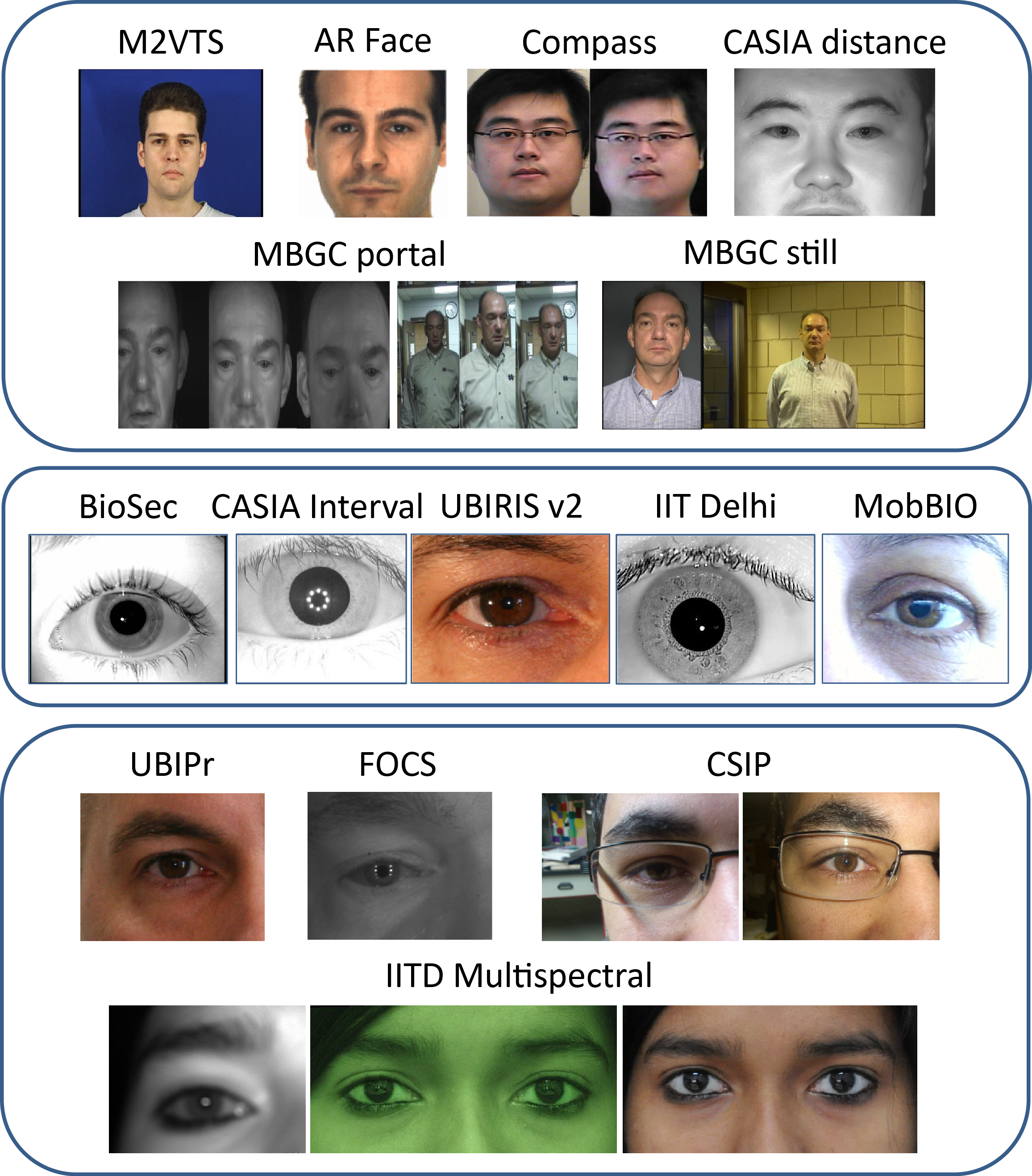
Fig. 2: Samples of databases used in periocular research. Top row: facial databases. Middle: iris databases. Bottom: periocular databases.

2.1 Facial Databases

M2VTS has video of people counting ’0’-’9’ in their native language and rotating the head left-right. AR has frontal view with different expressions, illumination, and occlusions (sun glasses, scarf). GTDB: Georgia Tech has frontal/titled faces with cluttered background, four expressions and lightning/scale change. Caltech has frontal pose under with different lighting/expressions/backgrounds. FERET: Facial Recognition Technology has variations of illumination, expression, pose (frontal, left/right), race, glasses, etc. CMU-H: CMU Hyperspectral has videos in the range 450nm-1100 nm, in steps of 10nm. Three halogen lamps surrounding the face was used individually one at a time, and all together (four lightning conditions). FRGC: Face Recognition Grand Challenge has controlled/uncontrolled and 3D images. Controlled images were taken in a studio setting, and uncontrolled images in hallways, atria, or outdoors, with varying lightning and distance. MORPH aging (Album1) has scanned mug-shots taken between 1962 and 1998, with age of the subjects ranging 15-68 years old. The gap between first and last images is from 46 days to 29 years. Images are near-frontal, with many types of illumination and eye occlusions. PUT has partially controlled illumination, uniform background and pose variation. Most images have neutral expression, although a small set has no constraints on pose or expressions. MBGC v2: Multiple Biometric Grand Challenge is organized into 3 challenges: $i$) Portal, $ii$) Still Face and $iii$) Video. Only $i$ and $ii$ have been used in periocular research. Portal data has subjects walking naturally through a portal, acquired simultaneously with NIR and VW video cameras. Therefore, many image perturbations appear. In the NIR sequences, some frames are too dark or too bright since the NIR lights shine only for a short time. Still Face data has high resolution images with controlled/uncontrolled illumination and frontal/non-frontal collected both in a studio environment and in hallways/outdoors. Plastic Surgery has one pre- and one post-surgery image for each person, both frontal, with proper illumination and neutral expression. ND-twins has images of twins under varying lighting (indoor/outdoor), expression (neutral/smile), and pose (frontal/non-frontal). Compass has four manners (neutral, smiling, eyes closed, facial occlusion) at two distances (10m and 20m) acquired with a pan-tilt-zoom (PTZ) camera. FG-NET Aging has subjects from multiple race, large variation of lighting, expression, and pose. The age range is 0-69 years, with images taken years apart. CASIA v4 Distance has high-resolution frontal NIR images with neutral expression acquired at $\sim$3 meters. FaceExpressUBI has seven expressions, with location/orientation of the camera and light sources changed between sessions.

2.2 Iris Databases

BioSec, CASIA Interval v3 and IIT Delhi v1.0 have NIR images acquired with close-up iris cameras. UBIRIS v2 has VW images acquired between 3-8 meters with a digital camera. The 1^st session has controlled conditions, and the 2^nd session was captured in a real-world setup (natural light, reflections, contrast change, defocus, occlusions, blur and off-angle). MobBIO has VW images from a Tablet PC with two lighting conditions, variable eye orientations and occlusions. Distance to the camera was kept constant. Annotation of the iris databases described, or a subset of them, have been made available (Alonso-Fernandez and Bigun, 2015; Hofbauer et al., 2014).

2.3 Periocular Databases

UBIPr was acquired with a digital camera, with distance, illumination, pose and occlusion variability. The distance varies between 4-8m in steps of 1m, with resolution from 501$\times$401 pixels (8m) to 1001$\times$801 (4m). FOCS: Face and Ocular Challenge Series has images from NIR videos of subjects walking through a portal (as in MBGC). A large number of images are of very poor quality, with high variations in illumination, out-of-focus blur, sensor noise, specular reflections, partially occluded iris and off-angle. The iris is very small ($\sim$50 pixels wide). IMP: IITD Multispectral Periocular has three spectrums: NIR, VW, and Night Vision. The NIR dataset is created with a close-up iris scanner, the VW dataset with a digital camera at 1.3 meters, and the night dataset with a handycam in night mode. CSIP: Cross-Sensor Iris and Periocular has images with four different smarphones. Ten different setups are included by capturing with both frontal/rear cameras and with/without the flash embedded in the device. The resolution of each camera is different, ranging from 640$\times$480 to 3264$\times$2448. Participants were captured at different sites with artificial, natural and mixed illumination. Noise factors include multiple scales, chromatic distortions, rotation, poor lightning, off-angle, defocus, and iris obstructions (including reflections).

Table 2: Overview of existing automatic eye/periocular detection and segmentation works. The acronyms of this table are fully defined in the text or in the referenced papers. Column ‘task’ stands for: D=Detection, S=Segmentation.

Approach	Features	Task	Training	Database	Best accuracy
Smeraldi and Bigün (2002)	Gabor filters	D	M2VTS (202 VW images)	M2VTS (349 VW images)	99.3% (M2VTS)
				XM2VTS (2388 VW images)	99% (XM2VTS)
Juefei-Xu and Savvides (2012)	Active Shape Models (ASM)	D	MBGC (VW images)	Compass (3200 VW images)	n/a
Uhl and Wild (2012)	Viola-Jones (VJ) detector of	D	n/a	CASIA distance v4 (282 NIR images)	96.4% (NIR)
	face sub-parts (OpenCV)			Yale-B (252 VW images)	99.2% (VW)
Zhou et al. (2012)	HSV color space + convex hull	D,S	n/a	UBIRIS v1 (1877 VW images)	n/a
Jillela et al. (2013)	Correlation filters	D	1000 eye images	FOCS (404 NIR images)	95%
Le et al. (2014)	LE-ASM + graph-cut	D,S	MBGC (500 VW images)	MBGC (200 still VW images)	F-measure: 99.4%
Mahalingam et al. (2014)	Correlation filters	D	n/a	HRT (VW images)	n/a
Oh et al. (2014)	HSV color space	D,S	n/a	UBIRIS v1 (1877 VW images)	n/a
Proenca (2014)	HSV+YCbCr color spaces	D,S	n/a	UBIRIS v2 /FRGC (2340/4360 VW images)	n/a
Proenca et al. (2014)	Texture/shape descriptors	S	UBIRIS v2 (35 VW images)	UBIRIS v2 (200 VW images)	97.5%
Alonso-Fernandez and Bigun (2015)	Symmetry filters	D	NO	6 iris datasets: 4 NIR, 2 VW	96% (NIR)
				(6932 NIR images, 3050 VW)	79% (VW)
Uzair et al. (2015)	VJ eye-pair + Hough	D	n/a	MBGC (VW, NIR), UBIPr (VW)	n/a
	VJ eye-pair + morphology		n/a	CMU-H	n/a

3 Detection and segmentation of the periocular region

Initial studies were focused on feature extraction only (with the periocular region manually extracted), but automatic detection and segmentation have increasingly become a research target in itself. Some works have applied a full face detector first such as the Viola-Jones (VJ) detector (Viola and Jones, 2004), e.g. Park et al. (2011) or Juefei-Xu and Savvides (2012), but successful extraction of the periocular region in this way relies on an accurate detection of the whole face. Using iris segmentation techniques may not be reliable under challenging conditions either (Jillela et al., 2013). On the other hand, eye detection can be a decisive pre-processing task to ensure successful segmentation of the iris texture in difficult images, as in the study by Jillela et al. (2013). Here, they used correlation filters to detect the eye center over the difficult FOCS database of subjects walking through a portal, achieving a 95% success rate. However, despite this good result in indicating the eye position, accuracy of the iris segmentation algorithms evaluated were between 51% and 90% Correlation filters were also used for eye detection in Mahalingam et al. (2014), although after applying the VJ face detector.

Table 2 summarizes existing research dealing with the task of locating the eye position directly, without relying on full-face or iris detectors. Uhl and Wild (2012) and Uzair et al. (2015) used the VJ detector of face sub-parts. Uzair et al. (2015) also experimented with the CMU hyperspectral database, which has images captured simultaneously at multiple wavelengths. Since the eye is centered in all bands, accuracy can be boosted by collective detecting the eye over all bands. Smeraldi and Bigün (2002) made use of Gabor features for eye detection and face tracking purposes by performing saccades across the image, whereas Alonso-Fernandez and Bigun (2014, 2015) proposed the use of symmetry filters tuned to detect circular symmetries. The latter has the advantage of not needing training, and detection is possible with a few 1D convolutions due to separability of the detection filters, built from derivatives of a Gaussian. Le et al. (2014) proposed a Local Eyebrow Active Shape Model (LE-ASM) to detect the eyebrow region directly from a given face image, with eyebrow pixels segmented afterwards using graph-cut based segmentation. ASMs were also used by Juefei-Xu and Savvides (2012) to automatically extract the periocular region, albeit after the application of a VJ full-face detector.

Recently, Proenca et al. (2014) proposed a method to label seve components of the periocular region (iris, sclera, eyelashes, eyebrows, hair, skin and glasses) by using seven classifiers at the pixel level, with each classifier specialized in one component. Pixel features used for classification included the following texture and shape descriptors: RGB/HSV/YCbCr values, Local Binary Patterns (LBP), entropy and Gabor features. Some works have proposed the extraction of features from the sclera region only, therefore requiring an algorithm to specifically segment this region. For this purpose, Oh et al. (2014), Proenca (2014) and Zhou et al. (2012) used the HSV/YCbCr color spaces. In these works, however, sclera detection is guided by a prior detection of the iris boundaries.

Table 3: Overview of existing periocular recognition works. The acronyms of this table are fully defined in the text or in the referenced papers.

			Best accuracy
Approach	Features evaluated	Test Database	Features	$\#$ eyes	EER	Rank-1
Smeraldi and Bigün (2002)	Gabor filters	M2VTS (349 VW images)	Gabor	one	0.3%	n/a
Park et al. (2009)	HOG, LBP, SIFT	FRGC (1704 VW images)	HOG/LBP/SIFT	one	21.78/19.26/6.96%	66.64/72.45/79.49%
Park et al. (2011)			HOG+LBP+SIFT	both	n/a	87.32%
Adams et al. (2010)	GEFE+LBP	FRGC (820 VW images)	GEFE+LBP	one/both	n/a	86.85% / 92.16%
		FERET (108 VW images)	GEFE+LBP	one/both	n/a	80.80% / 85.06%
Bharadwaj et al. (2010)	CLBP, GIST	UBIRIS v2 (7409 VW images)	CLBP	one/both	n/a	54.30% / 63.77%
			GIST	one/both	n/a	63.34% / 70.82%
			CLBP+GIST	one/both	n/a	n/a / 73.65%
Hollingsworth et al. (2010)	Human observers	Proprietary (120 subjects NIR)	Human	one	n/a	92%
Juefei-Xu et al. (2010, 2011)	LBP, WLBP, SIFT, DCT, Gabor	FRGC (16028 VW images)	FRGC: LBP+DWT	both	n/a	53.2%
	filters, Walsh masks, DWT, SURF		FRGC: LBP+DCT	both	n/a	53.1%
	Law Masks, Force Fields, LoG	FG-NET (1002 VW images)	FG-NET: WLBP	both	0.6%	100%
Miller et al. (2010b)	LBP	FRGC (1230 VW images)	LBP	one/both	0.10% / 0.09%	84.39% / 89.76%
		FERET (162 VW images)	LBP	one/both	0.22% / 0.23%	72.22% / 74.07%
Woodard et al. (2010a)	LBP	MBGC (1052 NIR portal images)	LBP	one	21%	92.5%
Woodard et al. (2010b)	LCH	FRGC (4100 VW images)	FRGC: RG	one/both	n/a	96.1% / 97.6%
	LBP		FRGC: LBP	one/both	n/a	95.6% / 97.6%
			FRGC: LCH+LBP	one/both	n/a	96.8% / 98.3%
		MBGC (911 NIR portal images)	MBGC: LBP	one	n/a	87%
Boddeti et al. (2011)	BGM	FOCS (9581 NIR images)	BGM	one	23.81%	94.2%
Dong and Woodard (2011)	eyebrow shape	MBGC (922 NIR portal images)	eyebrow shape	one	n/a	91%
		FRGC (800 VW images)	eyebrow shape	one	n/a	78%
Alonso-Fernandez and Bigun (2012, 2014, 2015)	Gabor filters	BioSec (1200 NIR images)	Gabor	one	10.56%	66%
		Casia Interval v3 (2655 NIR images)	Gabor	one	14.53%	n/a
		IIT Delhi v1.0 (2240 NIR images)	Gabor	one	2.5%	n/a
		MobBIO (800 VW images)	Gabor	one	12.32%	75%
		UBIRIS v2 (2250 VW images)	Gabor	one	24.4%	n/a
Hollingsworth et al. (2012)	Human observers	Proprietary (210 subjects VW, NIR)	VW/NIR: Human	one	n/a	88.4% / 78.8%
Jillela and Ross (2012)	SIFT, LBP	Plastic Surgery (1800 VW images)	LBP/SIFT/LBP+SIFT	both	n/a	45.6/48.1/63.9%
Joshi et al. (2012)	LBP	UBIRIS v2 (2400 VW images)	LBP	one	12.94%	81.03%
Juefei-Xu and Savvides (2012)	WLBP	Compass (3200 VW images)	WLBP	both	$\sim$10%	n/a
Oh et al. (2012)	LBP, PCA/LDA variants	FERET (354 VW images)	(2D)2LDA	one	$\sim$15%	n/a
Padole and Proenca (2012)	HOG, LBP, SIFT	UBIPr (10950 VW images)	HOG+LBP+SIFT	one	$\sim$20%	n/a
Ross et al. (2012)	HOG, m-SIFT, PDM	FOCS (9581 NIR images)	HOG/m-SIFT/PDM/all	one	33.2/27.2/23.9/18.8%	n/a
		FRGC (2272 VW images)	HOG/m-SIFT/PDM/m-SIFT+PDM	one	18.61/2.37/3.84/1.59%	n/a
Santos and Hoyle (2012)	LBP, SIFT	UBIRIS v2 (1000 VW images)	LBP/SIFT	one	31.87/32.09%	56.4/$\sim$8%
Tan and Kumar (2012)	SIFT, LBP, HOG, LMF	CASIA v4 Distance (2567 NIR images)	SIFT/LBP/HOG/LMF	one	n/a	$\sim$39/59/60/67%
Mahalingam and Ricanek (2013)	LBP, 3PLBP, H3PLBP	Morph (1690 VW images)	H3PLBP	both	n/a	33.2%
		FRGC (16000 VW images)	H3PLBP	both	n/a	97.51%
		Georgia Tech (750 VW images)	H3PLBP	both	n/a	92.4%
		ND Twins (6863 VW images)	H3PLBP	both	n/a	98.03%
Raghavendra et al. (2013)	LBP+SRC	Proprietary, light-field and digital	Light-field: LBP+SRC	one	12.04%	n/a
		cameras (420 VW images each)	Digital camera: LBP+SRC	one	16.21%	n/a
Smereka and Kumar (2013)	PDM, m-SIFT	FOCS (9581 NIR images)	PDM/m-SIFT	one	18.85/24.64%	97/97.75%
		UBIPr (10252 VW images)	PDM/m-SIFT	one	6.43/13.63%	99.75/96.24%
Uzair et al. (2013)	raw pixels, LBP, PCA, LBP+PCA	MGBC (3163 NIR portal images)	LBP+PCA	both	n/a	97.7%
Bakshi et al. (2014)	PIGP, CLBP, WLBP	UBIRIS v2 (11102 VW images)	PIGP/CLBP/WLBP	one	n/a	82.86/63.77/65.76%
Gangwar and Joshi (2014)	LPQ, LBP, Gabor filters	Caltech (VW images)	LPQ+Gabor magnitude	one/both	0.12/0.14%	n/a
		PUT (VW images)	LPQ	one/both	0.09/0.10%	n/a
		GTDB (VW images)	LPQ+Gabor magnitude	one/both	0.28/0.25%	n/a
		MBGC (VW still images)	LPQ+Gabor magnitude	one/both	0.22/0.20%	n/a
Jillela and Ross (2014)	LBP, NGC, JDSR	Proprietary iris (NIR), face (VW)	VW: LBP/NGC/JDSR/all	one	12/8/7/6%	n/a
Joshi et al. (2014)	Gabor-PPNN, DWT, LBP, HOG	MBGC (VW still images)	Gabor-PPNN	both	6.4%	75.8%
		GTDB (VW images)	Gabor-PPNN	both	5.9%	89.2%
		IITK (VW images)	Gabor-PPNN	both	15.5%	67.6%
		PUT (VW images)	Gabor-PPNN	both	4.8%	89.7%
Karahan et al. (2014)	SIFT, SURF, BRISK, ORB, LBP	FERET (2380 VW images)	SIFT+SURF	one	n/a	96.8%
Le et al. (2014)	Eyebrow shape	MBGC (4400 VW still images)	Eyebrow shape	both	n/a	85%
		AR Face (2800 VW images)	Eyebrow shape	both	n/a	76%
Mahalingam et al. (2014)	TPLBP, LBP, HOG	HRT ($>$1.2 mill. VW images)	TPLBP	both	35.21%	57.79%
Mikaelyan et al. (2014)	Symmetry patterns (SAFE)	BioSec (1200 NIR images)	SAFE	one	10.75%	n/a
Alonso-Fernandez et al. (2015)		CASIA Interval v3 (2655 NIR images)	SAFE	one	8.45%	n/a
		IITD (2240 NIR images)	SAFE	one	1.88%	n/a
		MobBIO (800 VW images)	SAFE	one	9.87%	n/a
		UBIRIS v2 (2250 VW images)	SAFE	one	24.56%	n/a
Nie et al. (2014)	PCA to: CRBM, SIFT, LBP, HOG	UBIPr (10252 VW images)	CRBM-PCA/all	one	10/6.4%	n/a/50.1%
Oh et al. (2014)	Directional projections (SRP)	UBIRIS v1 (1877 VW images)	SRP	one	6.52%	n/a
Proenca (2014)	LBP to eyelids region,	FRGC (4360 VW images)	LBP+EFD	one	$<$25%	n/a
	eyelids shape (EFD)	UBIRIS v2 (2340 VW images)	LBP+EFD	one	$<$24%	n/a
Proenca and Briceno (2014)	GC-EGM to: LBP+HOG+SIFT	FaceExpressUBI (90160 VW images)	GC-EGM	one	16%	n/a
Proenca et al. (2014)	LBP, HOG, SIFT	UBIRIS v2 (5551 VW images)	LBP+HOG+SIFT	one	9.5%	n/a
Raja et al. (2014)	BSIF	Proprietary, light-field and digital	Light-field: BSIF	one	3.39%	n/a
		cameras (420 VW images each)	Digital camera: BSIF	one	3.96%	n/a
Santos et al. (2014)	LBP, HOG, SIFT, ULBP, GIST	CSIP (2004 VW images)	LBP/HOG/SIFT/ULBP/GIST/all	one	30.5/30.8/34.3/25.9/16.3/15.5%	n/a
Sharma et al. (2014)	LBP, HOG, PHOG,	IMP: IITD Multispectral	VW : PHOG+NN	both	$\sim$8%	n/a
	FPLBP, PHOG+NN	(310 VW, 310 night, 620 NIR images)	night : PHOG+NN	both	$\sim$7%	n/a
			NIR : PHOG+NN	both	$\sim$3.5%	n/a
Bakshi et al. (2015)	PILP, SIFT, SURF	Bath (32000 NIR images)	any	one	n/a	100%
		CASIA Lamp v3 (16212 NIR images)	PILP/SIFT	one	n/a	100%
		UBIRIS v2 (11102 VW images)	PILP	one	n/a	87.62%
		FERET (14126 VW images)	PILP	one	n/a	85.8%
Uzair et al. (2015)	raw pixels, LBP, PCA, LBP+PCA	MGBC (NIR portal images)	LBP	one	n/a	99.8%
		MGBC (VW portal images)	LBP+PCA	one	n/a	98.5%
		CMU Hyperspectral	PCA	one	n/a	97.2%
		UBIPr (VW images)	LBP	one	n/a	99.5%

4 Recognition using periocular features

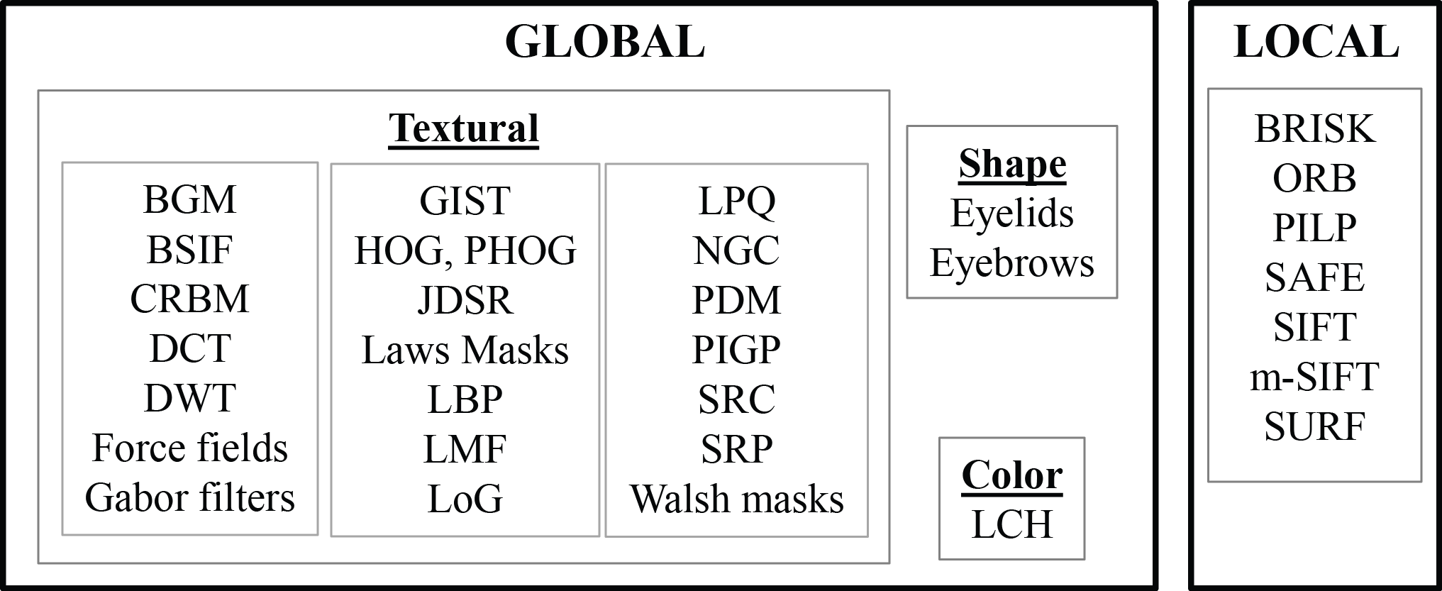
Fig. 3: Taxonomy of periocular features. The acronyms are fully defined in the text or in the referenced papers.

Several feature extraction methods have been proposed for periocular recognition, with a taxonomy shown in Figure 3. Existing features can be classified into: $i$) global features, which are extracted from the whole image or region of interest (ROI), and $ii$) local features, which are extracted from a set of discrete points, or key points, only. Table 3 gives an overview in chronological order of existing works for periocular recognition. The most widely used approaches include Local Binary Patterns (LBP) and, to a lesser extent, Histogram of Oriented Gradients (HOG) and Scale-Invariant Feature Transform (SIFT) key points. Over the course of the years, many other descriptors have been proposed. This section provides a brief description of the features used for periocular recognition (Section 4.1 and 4.2), followed by a review of the works mentioned in Table 3 (Section 4.3), highlighting their most important results or contributions. Due to pages limitation, we will omit references to the original works where features have been presented (unless they are originally proposed for periocular recognition in the mentioned reference). We refer to the references indicated for further information about the presented feature extraction techniques. Some preprocessing steps have been also used to cope with the difficulties found in unconstrained scenarios, such as pose correction by Active Appearance Models (AAM) (Juefei-Xu et al., 2011), illumination normalization (Juefei-Xu and Savvides, 2014; Nie et al., 2014), correction of deformations due to expression change by Elastic Graph Matching (EGM) (Proenca and Briceno, 2014), or color device-specific calibration (Santos et al., 2014). The use of subspace representation methods after feature extraction is also becoming a popular way either to improve performance or reducing the feature set, as mentioned next in this section. There are also periocular studies with human experts. Hollingsworth et al. (2010, 2012) evaluated the ability of (untrained) human observers to compare pairs of periocular images both with VW and NIR illumination, obtaining better results with the VW modality. They also tested three computer experts (LBP, HOG and SIFT), finding that the performance of humans and machines was similar.

4.1 Global features

Global approaches extract properties describing a entire ROI, such as texture, shape or color features. They are typically computed by dividing the image into a grid of patches (Figure 1, right) and extracting features in each patch. A global descriptor is then built by concatenating features from each patch into a single vector. This produces fixed length vectors, with matching between two images simply done by comparing these vectors with some distance measure, which is very time efficient.

4.1.1 Textural-based features

BGM: Bayesian Graphical Models were used by Boddeti et al. (2011). They adapted an iris matcher based on correlation filters applied to non-overlapping image patches. Patches of gallery and probe images are cross-correlated, and the output used to feed a Bayesian graphical model (BGM) trained to consider non-linear deformations and occlusions between images. BGM were also used by Smereka and Kumar (2013) and Ross et al. (2012), although called PDM or Probabilistic Deformation Models in these works.

BSIF: Binarized Statistical Image Features (Raja et al., 2014; Raghavendra et al., 2013) computes a binary code for each pixel by linearly projecting image patches onto a subspace, whose basis vectors are learnt from natural images using Independent Component Analysis (ICA). Since it is based on natural images, it is expected that BSIF encodes texture features more robustly than other methods that also produce binary codes, such as LBPs.

CRBM: Convolutional Restricted Boltzman Machines are a convolutional version of the Restricted Boltzman Machines, previously used in handwriting recognition, image classification, and face verification. CRBM, proposed for periocular recognition by Nie et al. (2014), is a generative stochastic neural network that learn a probability distribution over a set of inputs generated by filters which capture edge orientation and spatial connections between image patches.

DCT: Discrete Cosine Transform (Juefei-Xu et al., 2010) expresses data points by a sum of cosine functions oscillating at different frequencies (which in 2D corresponds to horizontal and vertical frequencies). The 2D-DCT is computed in image blocks of size $N\times N$ (with $N$=3,5,7…) and the $N^{2}$ coefficients are assigned as featureto the center pixel of the block.

DWT: Discrete Wavelet Transform was used by Juefei-Xu et al. (2010) and Joshi et al. (2014) with respect to the Haar wavelet, which, in 2D, leads to an approximation of image details in three orientations: horizontal, vertical and diagonal.

Force Field Transform (Juefei-Xu et al., 2010) employs an analogy to gravitational force. Each pixel exerts a ‘force’ on its neighbors inversely proportional to the distance between them, weighted by the pixel value. The net force at one point is the aggregate of the forces exerted by all other $5\times 5$ neighbors.

Gabor filters are texture filters selective in frequency and orientation. A set of different frequencies and orientations are usually employed. For example, Smeraldi and Bigün (2002) and Alonso-Fernandez and Bigun (2012, 2014, 2015) employed five frequencies and six orientations equally spaced in the log-polar frequency plane, achieving full coverage of the spectrum. Juefei-Xu et al. (2010) employed one frequency and four orientations, Gangwar and Joshi (2014) employed one frequency and one orientation only, and Joshi et al. (2014) employed five frequencies and six orientations. Lastly, Cao and Schmid (2014) used two frequencies and eight orientations, with Gabor responses further encoded by LBP operators (below).

GIST perceptual descriptors (Bharadwaj et al., 2010; Santos et al., 2014) consist of five perceptual dimensions related with scene description, correlated with the second-order statistics and spatial arrangement of structured image components: naturalness, which quantizes the vertical and horizontal edge distribution; openness, presence or lack of reference points; roughness, size of the largest prominent object; expansion, depth of the space gradient; and ruggedness, which quantizes the contour orientation that deviates from the horizontal.

HOG: Histogram of Oriented Gradients. In HOG, the gradient orientation and magnitude are computed in each pixel. The histogram of orientations is then built, with each bin accumulating corresponding gradient magnitudes. In PHOG or Pyramid of Histogram of Oriented Gradients, instead of using image patches, HOG is extracted from the whole image. Then, the image is split up several times like a quad-tree and all sub-images get their own HOG.

JDSR: Joint Dictionary-based Sparse Representation (Jillela and Ross, 2014). computes a compact dictionary using a set of training images. A new image is represented as a sparse linear combination of the dictionary elements. A similar approach is SRC, or Sparse Representation Classification (Raghavendra et al., 2013). An image is represented as a sparse linear combination of training images plus sparse errors due to perturbations. Images can be in original raw form or represented in any feature space. The features used included Eigenfaces, Laplacianfaces, Randomfaces, Fisherfaces, and downsampled versions of the raw image. Raghavendra et al. (2013) also tested BSIF and LBP features.

Laws masks were used by Juefei-Xu et al. (2010). Five 1D masks capturing shapes of level, edge, spot, wave and ripple were employed. In 2D, masks are 1D-convolved in all possible combinations with an image, thus producing 25 local features.

LBP: Local Binary Patterns were first introduced for texture classification, since they can identify spots, line ends, edges, corners and other patterns. For each pixel $p$, a $3\times 3$ neighborhood is considered. Every neighbor $p_{i}$ ($i$=1…8) is assigned a binary value of 1 if $p_{i}>p$, or 0 otherwise. The binary values are then concatenated into a 8-bits binary number, and the decimal equivalent is assigned to characterize the texture at $p$, leading to 2⁸=256 possible labels. The LBP values of all pixels within a given patch are then quantized into a 8-bin histogram. LBP is one of the most popular periocular matching techniques in the literature (Table 3), with many variants proposed. One is Uniform LBP or ULBP (Santos et al., 2014), used to reduce the length of the feature vector and achieve rotation invariance. A LBP is called uniform if it contains at most two bitwise transitions from 0 to 1 or vice-versa. A separate label is used for each uniform pattern, and all the non-uniform patterns are labeled with a single label, yielding to 59 different labels, instead of 256 as the regular LBP. The neighborhood can be also made larger to allow multi-resolution representations of the local texture pattern, leading to a circle of radius $R$, also called Circular LBP or CLBP (Bharadwaj et al., 2010; Bakshi et al., 2014). To avoid a large number of binary values as $R$ increases, only neighbors separated by certain angular distance may be chosen. In Three-Patch LBP or TPLBP/3PLBP (Mahalingam and Ricanek, 2013; Mahalingam et al., 2014), pixel $p$ is compared with the central pixel of two (non-adjacent) patches situated across a circle $R$. Application of 3PLBP to multiple image scales across a Gaussian pyramid leads to the Hierarchical Three-Patch LBP or H3PLBP (Mahalingam and Ricanek, 2013). Further extension to two circles $R_{1}$ and $R_{2}$ results in Four-Patch LBP or FPLBP (Sharma et al., 2014), involving four patches instead of three in the comparison. The use of subspace representation methods applied to LBPs is also very popular to reduce the feature set or improve performance, for example: Adams et al. (2010), Juefei-Xu et al. (2011), Oh et al. (2012), Uzair et al. (2013, 2015) and Nie et al. (2014). Other works have also proposed to apply LBP upon other feature extraction itself, for example Juefei-Xu et al. (2010); Juefei-Xu and Savvides (2012), Bakshi et al. (2014) or Cao and Schmid (2014).

LMF: Leung-Mallik filters is a set of filters constructed from Gaussian, Gaussian derivatives and Laplacian of Gaussian at different orientations and scales. In the experiments by Tan and Kumar (2012), filter responses from an image training set were clustered by $k$-means to construct a texton dictionary. The clusters (texton) producing the lowest EER were then used to classify test images.

LoG: Laplacian of Gaussian filter is an edge detector, used by Juefei-Xu et al. (2010) for periocular recognition.

LPQ: Local Phase Quantization (Gangwar and Joshi, 2014) extracts phase statistics of local patches by selective frequency filters in the Fourier domain. The phases of the four low-frequency coefficients are quantized in four bins.

NGC: Normalized Gradient Correlation (Jillela and Ross, 2014) computes in the Fourier domain the normalized correlation between the gradients of two images in pair-wise patches.

PIGP: Phase Intensive Global Pattern (Bakshi et al., 2014) computes the intensity variation of pixel-neighborhoods with respect to different phases by convolution with a bank of $3\times 3$ filters. The filters have ‘U’ shape when seen in 3D, with different rotations corresponding to the different phases. Four different angles between 0 and 3$\pi$/4 in steps of $\pi$/4 were considered.

SRP: Structured Random Projections (Oh et al., 2014) encode horizontal and vertical directional features by means of 1D horizontal and vertical binary vectors (projection elements). Such elements have a single group of contiguous ‘1’ values, with the location of ‘1’s’ randomly determined. The number $k$ of projection elements and the length $l$ of contiguous ‘1’s’ are to be fixed experimentally, with $k$=10 and $l$=3,6,…150 tested.

Walsh masks are convolution filters which only contain +1 and -1 values, thus capturing the binary characteristics of an image in terms of contrast. $N$ different 1D-filters of $N$ elements are produced ($N$=3,5,7…) and combined in all possible pairs, yielding to $N^{2}$ 2D-filters. Walsh masks were used by Juefei-Xu et al. (2010), Juefei-Xu and Savvides (2012) and Bakshi et al. (2014) to compute the Walsh-Hadamard Transform based LBPs (WLBP), which consists of extracting LBPs from the input image after being filtered with Walsh masks.

4.1.2 Shape-based features

Eyelids shape descriptors (Proenca, 2014) extract several properties from the polynomial encoding each eyelid, including: accumulated curvature at point $i$ (out of $t$), defined as $\sum\nolimits_{j=1}^{i}{\frac{{\partial^{2}y_{j}}}{{\partial x^{2}}}}/\sum\nolimits_{j=1}^{t}{\frac{{\partial^{2}y_{j}}}{{\partial x^{2}}}}$; shape context, represented by the histogram $h_{i}$ of $(x_{i}-x_{j},y_{i}-y_{j})$ at each point $(x_{i},y_{i})$, $\forall j\neq i$; and the Elliptical Fourier Descriptors (EFD) parameterizing $y_{i}$ coordinates of the eyelids. Proenca (2014) also applied LBP to the eyelids region only.

Eyebrows shape was studied by Dong and Woodard (2011) and Le et al. (2014). Dong and Woodard (2011) encoded rectangularity, eccentricity, isoperimetric quotient, area percentage of different sub-regions, and critical points (comprising the right/left-most points, the highest point and the centroid). Le et al. (2014) proposed the use of shape context histograms encoding the distribution of eyebrow points relative to a given (reference) point, and the Procrustes analysis representing the eyebrow shape asymmetry.

4.1.3 Color-based features

LCH: Local Color Histograms from image patches were used by Woodard et al. (2010b). They experimented with RGB and HSV spaces and their sub-spaces, finding that the RG (red-green) color space outperformed the other, with a $4\times 4$ histogram giving better results than coarser or finer resolutions. Thus each $4\times 4$ histogram provides a 16 element feature vector per patch. LCH were also used by Lyle et al. (2012) for gender and ethnicity classification using periocular data (Section 7).

4.2 Local features

In local approaches, a sparse set of characteristic points (called key points) is detected first. Local features encode properties of the neighborhood around key points only, leading to local key point descriptors. Since the number of detected key points is not necessarily the same in each image, the resulting feature vector may not be of constant length. Therefore, the matching algorithm has to compare each key point of one image against all key points of the other image to find a pair match, thus increasing the computation time. The output from the matching function is typically the number of matched points, although a distance measurement between pairs may also be returned. To achieve scale invariance, key points are usually detected at different scales. Different key point detection algorithms exist, with some of the feature extraction methods of this section also having its own key point extraction method. For example, detection of key points with the SIFT feature extractor relies on a difference of Gaussians (DOG) function in the scale space, whereas detection with SURF is based on the Hessian matrix, but relying on integral images to speed up computations. Newer algorithms such as BRISK and ORB claim to provide an even faster alternative to SIFT or SURF key point extraction methods. Karahan et al. (2014) employs one key point extraction method (SURF), and then compute the SIFT, SURF, BRISK and ORB descriptors from these key points. Other periocular works like Karahan et al. (2014), Mikaelyan et al. (2014) and Alonso-Fernandez and Bigun (2015) extract key points descriptors at selected sampling points in the center of image patches only, resembling the grid-like analysis of global approaches (Figure 1, right) but using local features. This way, no key point detection is carried out, and the obtained feature vector is of fixed size. The following local descriptors have been proposed in the literature for periocular recognition.

BRISK: Binary Robust Invariant Scalable Key points descriptor is composed of a binary string by concatenating the results of simple brightness comparison tests. BRISK applies a sampling pattern of $N$=60 locations equally spaced on circles concentric with the key point. The origin of the sampling pattern is rotated according to the gradient angle around the key point to achieve rotation invariance. The intensity of all possible short-distance pixel pairs $p_{i}$ and $p_{j}$ of the sampling pattern is then compared, assigning a binary value of 1 if $p_{i}>p_{j}$, and 0 otherwise. The resulting feature vector at each key point has 512 bits. BRISK is employed for periocular recognition by Karahan et al. (2014).

ORB: Oriented FAST and Rotated BRIEF is based on the FAST corner detector and the visual descriptor BRIEF (Binary Robust Independent Elementary Features). As in BRISK, BRIEF also uses binary tests between pixels. Pixel pairs are considered from an image patch of size $S\times S$. The original BRIEF deals poorly with rotation, so in ORB it is proposed to steer the descriptor according to the dominant rotation of the key point (obtained from the first order moments). The parameters employed in ORB are $S$=31 and a vector length of 256 bits per key point. ORB was used for periocular recognition by Karahan et al. (2014).

PILP: Phase Intensive Local Pattern was used by Bakshi et al. (2015), following the work in Bakshi et al. (2014) where they presented PIGP (Phase Intensive Global Pattern). PILP uses a similar filter bank than PIGP, but used for key point extraction, rather than for feature encoding. Size of the filters varies from $3\times 3$ to $9\times 9$, to allow to cope with scale variations. This way, key points are the local extrema among pixels in its own window and windows in its neighboring phases. Feature extraction is then done by computing a gradient orientation histogram in the neighborhood of each keypoint, in a similar way than SIFT descriptor, below.

SAFE: Symmetry Assessment by Feature Expansion (Mikaelyan et al., 2014; Alonso-Fernandez and Bigun, 2015) describes neighborhoods around key points by projection onto harmonic functions which estimates the presence of various symmetric curve families. The iso-curves of such functions are highly symmetric w.r.t. the key points and the estimated coefficients have well defined geometric interpretations. The detected patterns resemble shapes such as parabolas, circles, spirals, etc. Detection is done in concentric circular bands of different radii around key points, with radii log-equidistantly sampled. Extracted features therefore quantify the presence of pattern families in annular rings around each key point.

SIFT: Scale Invariant Feature Transformation. Together with LBP, SIFT is the most popular matching technique employed in the literature (Table 3). SIFT encodes local orientation via histograms of gradients around key points. The dominant orientation of a key point is first obtained by the peak of the gradient orientation histogram in a $16\times 16$ window. The key point feature vector of dimension $4\times 4\times 8=128$ is then obtained by computing 8-bin gradient orientation histograms (relative to the dominant orientation to achieve rotation invariance) in $4\times 4$ sub-regions around the key point. m-SIFT (modified SIFT) is a SIFT matcher where additional constraints are imposed to the angle and distance of matched key points (Ross et al., 2012; Smereka and Kumar, 2013).

SURF: Speeded Up Robust Features was aimed at providing a detector and feature extractor faster than SIFT and other local feature algorithms. Feature extraction is done over a $4\times 4$ sub-region around the key point (relative to the dominant orientation) using Haar wavelet responses. SURF is employed for periocular recognition by Juefei-Xu et al. (2010), Karahan et al. (2014) and Bakshi et al. (2015).

4.3 Literature review of periocular recognition works

Periocular recognition started to gain popularity after the studies by Park et al. (2009, 2011). Some pioneering works can be traced back to 2002 (Smeraldi and Bigün, 2002), although authors here did not call the local eye area ‘periocular’. The approach by Park et al. (2011) combined global and local features, concretely LBP, HOG and SIFT. Reported performance of such study was fairly good, setting the framework for the use of the periocular modality. Many works have followed this approach as inspiration, with LBPs and their variations being particularly extensive in the literature (Miller et al., 2010b; Woodard et al., 2010a, b; Tan and Kumar, 2012; Mahalingam and Ricanek, 2013; Karahan et al., 2014). The studies of (Woodard et al., 2010a, b) used for the first time NIR data (MBGC portal video), although they selected usable frames (higher quality) which mostly are in the earlier part of the video, where scale change is not substantial. Boddeti et al. (2011) also presented experiments over NIR portal data from the more difficult FOCS database, but with a different descriptor (BGM). Mahalingam and Ricanek (2013) also evaluated the impact of covariates such as pose, expression, template aging, glasses and eyelids occlusion. Some works have also employed other features in addition to LBPs (Woodard et al., 2010b; Tan and Kumar, 2012; Karahan et al., 2014). Woodard et al. (2010b) employed LCH (RG color histograms), reporting the best accuracy up to that date with the FRGC database of VW images. Tan and Kumar (2012) proposed Leung-Mallik filters (LMF) as texture descriptors over the CASIA v4 Distance database of NIR images. Karahan et al. (2014) evaluated LBP, SIFT, and other local descriptors including SURF, BRISK and ORB over the FERET database. The use of subspace representation methods applied to raw pixels or LBP features is also becoming a popular way either to improve performance or reducing the feature set (Adams et al., 2010; Oh et al., 2012; Uzair et al., 2013; Juefei-Xu and Savvides, 2014; Nie et al., 2014; Uzair et al., 2015). LBP has been also used in other works analyzing for example the impact of plastic surgery (Jillela and Ross, 2012) or gender transformation (Mahalingam et al., 2014) on periocular recognition (see Section 7).

Inspired by Park et al. (2009), Juefei-Xu et al. (2010) extended the experiments with additional global and local features to a significant larger set of the FRGC database with less ideal images (thus the lower accuracy w.r.t. previous studies): WLBP, Law s Masks, DCT, DWT, Force Field transform, SURF, Gabor filters and LoG filters. They later addressed the problem of aging degradation on periocular recognition using the FG-NET database (Juefei-Xu et al., 2011), reported to be an issue even at small time lapses (Park et al., 2011). To obtain age invariant features, they first performed preprocessing schemes, such as pose correction by Active Appearance Models (AAM), illumination and periocular region normalization. In a later work, Juefei-Xu and Savvides (2012) also applied WLBPs to study periocular recognition with data from a pan-tilt-zoom (PTZ) camera. As in the study above, they employed different schemes to correct illumination and pose variations.

The mentioned work by Smeraldi and Bigün (2002) with Gabor filters served as inspiration to Alonso-Fernandez and Bigun (2012, 2014, 2015) to carry out periocular experiments with several iris databases in NIR and VW, as well as a comparison with the iris modality (Section 6). A variation of this algorithm was fused with the SIFT descriptor, obtaining a leading position in the First ICB Competition on Iris Recognition, ICIR2013 (Zhang et al., 2014). They later proposed a matcher based on Symmetry Assessment by Feature Expansion (SAFE) descriptors (Mikaelyan et al., 2014; Alonso-Fernandez and Bigun, 2015), which describes neighborhoods around key-points by estimating the presence of various symmetric curve families. Gabor filters were also used by Gangwar and Joshi (2014) in their work presenting Local Phase Quantization (LPQ) as descriptors for periocular recognition. Joshi et al. (2014) also employed Gabor features over four different VW databases, with features reduced by Direct Linear Discriminant Analysis (DLDA) and further classified by a Parzen Probabilistic Neural Network (PPNN).

Bharadwaj et al. (2010) evaluated CLBP and GIST descriptors. They used the UBIRIS v2 database of uncontrolled VW iris images which includes a number of perturbations intentionally introduced (see Section 2). A number of subsequent works have also made use of UBIRIS v2 (Joshi et al., 2012; Santos and Hoyle, 2012; Bakshi et al., 2014; Proenca, 2014; Proenca et al., 2014; Bakshi et al., 2015). Joshi et al. (2012) used UBIRIS v2 in their comparison of iris and periocular modalities (Section 6), obtaining better results than Bharadwaj et al. (2010) using just LBPs, although over a smaller set of images. Santos and Hoyle (2012) used LBPs and SIFT as by Park et al. (2009) in their study combining iris and periocular modalities (Section 6). Bakshi et al. (2014) proposed global PIGP features, outperforming the Rank-1 performance of any previous study using UBIRIS v2. They later proposed local PILP features (Bakshi et al., 2015), reporting the best Rank-1 periocular performance to date with UBIRIS v2. Proenca (2014) studied the fusion of iris and periocular biometrics (Section 6). Periocular features were extracted from the eyelids region only, consisting of the fusion of LBPs and eyelids shape descriptors. In a subsequent study, Proenca et al. (2014) proposed a method to label seven components of the periocular region (see Section 3) with the purpose of demonstrating that regions such as hair or glasses should be avoided since they are unreliable for recognition (Section 5). They also proposed to use the center of mass of the cornea as reference point to define the periocular ROI, rather than the pupil center, which is much more sensitive to changes in gaze. Finally, Oh et al. (2014) used the first version of UBIRIS in their study presenting directional projections or Structured Random Projections (SRP) as periocular features.

Other shape features have been also proposed, such as eyebrow shape features, with surprisingly accurate results as a stand-alone trait. Indeed, eyebrows have been used by forensic analysts for years to aid in facial recognition (Le et al., 2014), suggested to be the most salient and stable features in a face (Sadr et al., 2003). Dong and Woodard (2011) studied several geometrical shape properties over the MGBC/FRGC databases. They also used the extracted eyebrow features for gender classification (see Section 7). Le et al. (2014) proposed an eyebrow shape-based identification system, together with a eyebrow segmentation technique (presented in Section 3).

Padole and Proenca (2012) presented the first periocular database in VW range specifically acquired for periocular research (UBIPr). They also proposed to compute the ROI w.r.t. the midpoint of the eye corners (instead of the pupil center), which is less sensitive to gaze variations, leading to a significant improvement (EER from $\sim$30% to $\sim$20%). Posterior studies have managed to improve performance over the UBIPr database using a variety of features (Smereka and Kumar, 2013; Nie et al., 2014). The UBIPr database is also used by Uzair et al. (2015) in their extensive study evaluating data in VW (UBIPr, MBGC), NIR (MBGC) and multi-spectral (CMU-H database) range, with the reported Rank-1 results being the best published performance to date for the four databases employed. A new database of challenging periocular images in VW range (CSIP) was presented recently by Santos et al. (2014), the first one made public captured with smartphones. The paper proposed a device-specific calibration method to compensate for the chromatic disparity, as result of the variability of camera sensors and lenses used by different mobile phones. They also compared and fused the periocular and iris modalities (Section 6).

Another database captured specifically for cross-spectral periocular research (IMP) was also recently presented by Sharma et al. (2014), containing data in VW, NIR and night modalities. To match cross-spectral images, they proposed neural networks (NN) to learn the variability caused by different spectrums, with several variations of LBP and HOG tested as features. Cross-spectral recognition was also addressed by Jillela and Ross (2014) using a proprietary database of NIR and VW images. Finally, Raghavendra et al. (2013) and Raja et al. (2014) presented a database in VW range acquired with a new type of camera, a Light Field Camera (LFC), which provides multiple images at different focus in a single capture. LFC overcomes one important disadvantage of sensors in VW range, which is guaranteeing a good focused image. Unfortunately, the database has not been made available. Individuals were also acquired with a conventional digital camera, with a superior performance observed with the LFC camera. New periocular features were also presented in the two studies. Raghavendra et al. (2013) proposed Sparse Representation Classification (SRC), previously used in face recognition. Raja et al. (2014) proposed Binarized Statistical Image Features (BSIF) for periocular recognition, further utilized as features of the SRC method described. Both Raghavendra et al. (2013) and Raja et al. (2014) tested the fusion of iris and periocular modalities as well (Section 6).

5 Best regions for periocular recognition

Most periocular algorithms work in a holistic way, defining a ROI around the eye (usually a rectangle) which is fully used for feature extraction. Such holistic approach implies that some components not relevant for identity recognition, such as hair or glasses, might erroneously bias the process (Proenca et al., 2014). It can also be the case that a feature is not equally discriminative in all parts of the periocular region.

The study by Hollingsworth et al. (2012) identified which ocular elements humans find more useful for periocular recognition. With NIR images, eyelashes, tear ducts, eye shape and eyelids, were identified as the most useful, while skin was the less useful. But for VW data, blood vessels and skin were reported more helpful than eye shape and eyelashes. Similar studies have been done with automatic algorithms (Smereka and Kumar, 2013; Alonso-Fernandez and Bigun, 2014), with results in consonance with the study with humans, despite using several machine algorithms based on different features, and different databases. With NIR images, regions around the iris (including the inner tear duct and lower eyelash) were the most useful, while cheek and skin texture were the less important. With VW images, on the other hand, the skin texture surrounding the eye was found very important, with the eyebrow/brow region (when present) also favored in visible range. This is in line with the assumption largely accepted in the literature that the iris texture is more suited to NIR illumination (Daugman, 2004), whereas the periocular modality is best for VW illumination (Hollingsworth et al., 2012; Woodard et al., 2010b). This seems to be explained by the fact that NIR illumination reveals the details of the iris texture, while the skin reflects most of the light, appearing over-illuminated (see for example ‘BioSec’ or other NIR iris examples in Figure 2); on the other hand, the skin texture is clearly visible in VW range, but only irises with moderate levels of pigmentation image reasonably well in this range (Bowyer et al., 2007).

Park et al. (2011) carried out experiments by masking parts of the periocular area over VW images of the FRGC database. They found that inclusion of eyebrows is beneficial for a better identification performance, with differences in Rank-1 of 8-19%, depending on the machine expert. Similarly, they observed that occluding ocular information (iris and sclera) deteriorates the performance, with reductions in Rank-1 accuracy of up to 41%. In the same direction, Oh et al. (2012) focused on the inclusion of a significant part of the cheek region over VW images of the FERET database, finding that it does not contain significant discriminative information while it increases the image size. Including the eyebrows and the ocular region was also found to be beneficial in this study, corroborating the results of Park et al. (2011). Recently, Proenca et al. (2014) proposed a method to label seven components of the periocular region: iris, sclera, eyelashes, eyebrows, hair, skin and glasses. The usefulness of such segmentation is demonstrated by avoiding hair and glasses in the feature encoding and matching stages, obtaining performance improvements by fusion of LBP, HOG and SIFT features (Park et al., 2011) over the UBIRIS v2 database of VW images (EER reduced from 12.8% to 9.5%).

Table 4: Overview of existing works on comparison and fusion of the periocular modality with other biometric modalities. The acronyms of this table are fully defined in the text or in the referenced papers. Features with best accuracy are those giving the best fusion results. If no fusion results are available, they indicate the best features of each individual modality. The following acronyms are not defined elsewhere: ‘w-sum’=‘weighted sum’, ‘LR’=‘logistic regression’, ‘NN’=‘Neural Networks’, ‘TERELM’=‘Total Error Rate Minimization’, ‘LG’=‘Log-Gabor’.

COMPARISON WITH THE IRIS MODALITY
					Best accuracy
	Features with best accuracy		Fusion		Periocular		Iris		Fusion
Approach	Periocular	Iris	method	Test Database	EER	Rank-1	EER	Rank-1	EER	Rank-1
Woodard et al. (2010a)	LBP	Gabor	w-sum	MBGC (1052 NIR portal images)	21%	92.5%	32%	13.81%	18%	96.5%
Boddeti et al. (2011)	BGM	Gabor	-	FOCS (9581 NIR images)	23.81%	94.2%	30.8%	88.7%	n/a	n/a
Joshi et al. (2012)	LBP	wavelets	DLDA	UBIRIS v2 (2400 VW images) +	12.94%	81.03%	12.07%	88.79%	6.9%	96.55%
			mean	CASIA Interval (2400 NIR images)					9.5%	83.62%
Ross et al. (2012)	HOG, m-SIFT, PDM	LG	-	FOCS (9581 NIR images)	18.8%	n/a	33.1%	n/a	n/a	n/a
Santos and Hoyle (2012)	LBP, SIFT	wavelets, Gabor	LR	UBIRIS v2 (1000 VW images)	31.87%	56.4%	23.12%	41.9%	18.48%	74.3%
Tan and Kumar (2012)	SIFT, LMF	LG	w-sum	CASIA v4 Distance (2567 NIR images)	n/a	$\sim$67%	n/a	$\sim$54%	n/a	84.5%
Raghavendra et al. (2013)	LBP+SRC	LBP+SRC	w-sum	Light-field camera (420 VW images)	12.04%	n/a	1.2%	n/a	0.81%	n/a
				Digital camera (420 VW images)	16.21%	n/a	8.24%	n/a	7.45%	n/a
Proenca (2014)	LBP + eyelids shape	MLDF	sum	FRGC (4360 VW images)	$<$25%	n/a	$<$11%	n/a	$<$8.5%	n/a
				UBIRIS v2 (2340 VW images)	$<$24%	n/a	$<$11%	n/a	$<$9%	n/a
Raja et al. (2014)	BSIF	BSIF	w-sum	Light-field camera (420 VW images)	3.39%	n/a	0.72%	n/a	0.61%	n/a
				Digital camera (420 VW images)	3.96%	n/a	3.46%	n/a	2.02%	n/a
Santos et al. (2014)	LBP+HOG+SIFT+ULBP+GIST	Gabor filters	NN	CSIP (2004 VW images)	15.5%	n/a	34.4%	n/a	14.5%	n/a
Alonso-Fernandez and Bigun (2014, 2015)	Gabor filters	LG	mean	BioSec (1200 NIR images)	10.56%	66%	1.12%	98%	1.96%	96%
	Gabor filters	LG	mean	Casia Interval v3 (2655 NIR images)	14.53%	n/a	0.67%	n/a	2.38%	n/a
	Gabor filters	LG	mean	IIT Delhi v1.0 (2240 NIR images)	2.5%	n/a	0.59%	n/a	1.2%	n/a
	Gabor filters	LG	mean	MobBIO (800 VW images)	12.32%	75%	18.81%	56%	11%	77%
	Gabor filters	LG	mean	UBIRIS v2 (2250 VW images)	24.4%	n/a	34.94%	n/a	22.41%	n/a
Alonso-Fernandez et al. (2015)	Gabor, SAFE, SIFT	LG, DCT	mean	BioSec (1200 NIR images)	8.5%	n/a	1.12%	n/a	0.75%	n/a
Mikaelyan et al. (2014)	SAFE, SIFT	LG, DCT, SIFT	mean	Casia Interval v3 (2655 NIR images)	7.52%	n/a	0.67%	n/a	0.51%	n/a
	SIFT	LG	mean	IIT Delhi v1.0 (2240 NIR images)	0.8%	n/a	0.59%	n/a	0.38%	n/a
	Gabor, SAFE, SIFT	LG	mean	MobBIO (800 VW images)	8.73%	n/a	18.81%	n/a	6.75%	n/a
	Gabor, SAFE, SIFT	LG, DCT, SIFT	mean	UBIRIS v2 (2250 VW images)	24.4%	n/a	35.61%	n/a	15.17%	n/a
COMPARISON WITH THE SCLERA MODALITY
					Best accuracy
	Features with best accuracy		Fusion		Periocular		Sclera		Fusion
Approach	Periocular	Sclera	method	Test Database	EER	Rank-1	EER	Rank-1	EER	Rank-1
Oh et al. (2014)	SRP	MLBP	TERELM	UBIRIS v1 (1877 VW images)	6.52%	n/a	8.44%	n/a	3.26%	n/a
COMPARISON WITH THE FACE MODALITY
					Best accuracy
	Features with best accuracy		Fusion		Periocular		Face		Fusion
Approach	Periocular	Face	method	Test Database	EER	Rank-1	EER	Rank-1	EER	Rank-1
Smeraldi and Bigün (2002)	Gabor filters	Gabor filters	w-sum	M2VTS (349 VW images)	0.3%	n/a	0.13%	n/a	n/a	n/a
Miller et al. (2010a)	LBP	LBP	-	FRGC (VW images)	n/a	99.5%	n/a	99.75%	n/a	n/a
				FRGC - blur (kernel=7 pix, $\sigma$=1.5)	n/a	77.86%	n/a	31.09%	n/a	n/a
				FRGC - downsampling (40%)	n/a	97.76%	n/a	70.40%	n/a	n/a
				FRGC - uncontrolled lightning	n/a	11.17%	n/a	12.18%	n/a	n/a
Park et al. (2011)	HOG, LBP, SIFT	FaceVACS	-	FRGC (1704 VW images)	n/a	87.32%	n/a	99.77%	n/a	n/a
				FRGC - partial face	n/a	$\sim$84%	n/a	39.55%	n/a	n/a
Jillela and Ross (2012)	SIFT, LBP	VeriLook, PittPatt	w-sum	Plastic Surgery (1800 VW images)	n/a	63.9%	n/a	85.3%	n/a	87.4%
Mahalingam et al. (2014)	TPLBP	TPLBP	-	HRT ($>$1.2 mill. VW images)	35.21%	57.79%	38.60%	46.49%	n/a	n/a

6 Comparison and fusion with other modalities

Periocular biometrics has rapidly evolved to competing with face or iris recognition. The periocular region appears in face or iris images, therefore comparison and/or fusion with these modalities has been also proposed. This section gives an overview of these works, with a summary provided in Table 4. Under difficult conditions, such as acquisition portals (Woodard et al., 2010a; Boddeti et al., 2011; Ross et al., 2012), distant acquisition (Tan and Kumar, 2012), smartphones (Santos et al., 2014), webcams or digital cameras (Alonso-Fernandez and Bigun, 2015; Alonso-Fernandez et al., 2015), the periocular modality is shown to be clearly superior to the iris modality, mostly due to the small size of the iris or the use of visible illumination. Visible illumination is predominant in relaxed or uncooperative setups due to the impossibility of using NIR illumination. Iris texture is more suited to the NIR spectrum, since this type of lightning reveals the details of the iris texture (Daugman, 2004), while the skin reflects most of the light, appearing over-illuminated. On the other hand, the skin texture is clearly visible in VW range, but only irises with moderate levels of pigmentation image reasonably well in this range (Bowyer et al., 2007). Nevertheless, despite the poor performance shown by the iris in the visible spectrum, fusion with periocular is shown to improve the performance in many cases as well (Santos and Hoyle, 2012; Alonso-Fernandez et al., 2015). Similar trends are observed with face. Under difficult conditions, such as blur or downsampling, the periocular modality performs considerably better (Miller et al., 2010a). It is also the case of partial face occlusions, where performance of full-face matchers is severely degraded (Park et al., 2011).

6.1 Iris Modality

Woodard et al. (2010a) evaluated NIR portal videos of the MBGC database. The periocular modality showed considerable superiority, with the performance further improved by the fusion, demonstrating the benefits of fusing periocular and iris information in non-ideal conditions. Boddeti et al. (2011) and Ross et al. (2012) also used NIR portal data from the FOCS database. Despite using other feature extraction methods, they also concluded that the periocular modality is considerable superior than the iris modality in such difficult data. Santos and Hoyle (2012) utilized VW images from the UBIRIS v2 database, which has several perturbations deliberately introduced. As with the above studies with NIR data, combining periocular and iris features improved the overall performance over difficult VW data too. Joshi et al. (2012) used a virtual database, with VW periocular data from UBIRIS v2 and NIR iris data from CASIA Interval. Fusion was carried out at the feature level, with vectors from the two modalities pooled together. They also tested a simple mean fusion rule at the score level, which resulted in a smaller performance improvement. Tan and Kumar (2012) used at-a-distance images from CASIA v4 Distance database, with a considerable performance improvement w.r.t. the individual modalities. Raghavendra et al. (2013) used a VW Light Field Camera (LFC), which provides multiple images at different focus in a single capture. Individuals were also acquired with a conventional digital camera. A superior performance with the LFC camera was observed with both modalities, which was reinforced even more with the fusion. The same databases were used in a posterior study by Raja et al. (2014), obtaining even better performance. Santos et al. (2014) used their new CSIP database, acquired with 4 different mobile telephones in 10 different setups. Using a sensor-specific color correction technique, they achieved a periocular EER cross-sensor performance of 15.5%. Despite the poor performance of Gabor wavelets applied to the iris modality (34.4%), they achieved a 14.5% EER with the fusion of the two modalities. Alonso-Fernandez and Bigun (2015) evaluated their Gabor-based periocular system and a set of four iris matchers. They used five different databases, three in NIR and two in VW range, observing that performance of the iris matchers was, in general, much better than the periocular matcher with NIR data, and the opposite with VW data. This is in tune with the literature, which indicates that the iris modality is more suited to NIR illumination (Daugman, 2004), whereas the periocular modality is best for VW illumination (Hollingsworth et al., 2012; Woodard et al., 2010b). With regards to the fusion, despite the poor performance of the iris matchers with VW data, its fusion with the periocular system resulted with important performance improvements. This is remarkable given the adverse acquisition conditions and the small resolution of the VW databases used. They further extended the study with their SAFE matcher (Mikaelyan et al., 2014), and a SIFT matcher. Here, the availability of more machine experts allowed to obtain performance improvements through the fusion also with NIR databases, something not observed in their previous studies. Proenca (2014) proposed the fusion of a iris matcher based on multi-lobe differential filters (MLDF), with a periocular expert that parameterizes the shape of eyelids, over VW data of FRGC and UBIRIS v2 databases, with an average 20% of EER improvement.

6.2 Sclera Modality

Some works have also made use of features from the sclera region. Oh et al. (2014) proposed to combine periocular and sclera features for identity verification, observing a significant improvement in EER after the fusion using UBIRIS v1.

6.3 Face Modality

Smeraldi and Bigün (2002) presented a face recognition expert based on Gabor filters applied to each facial landmark (eyes and mouth), with a different classifier employed in each landmark. Face authentication was performed by fusion of the three classifier’s output. This way, the face expert is really a fusion of two eye (periocular) experts and one mouth expert. Miller et al. (2010a) used LBP on the FRGC database, extracted both from the periocular region and from the full face. Rather than the best accuracy obtained (first sub-row in Table 4), the interest relies on the impact of the input image quality, demonstrating that, at extreme values of blur or down-sampling, periocular recognition performed significantly better than face. On the other hand, both face and periocular under uncontrolled lighting were very poor, indicating that LBPs are not well suited for this scenario. Another study of the effect of non-ideal conditions was also carried out by Park et al. (2011). They masked the face region below the nose to simulate partial face occlusion, showing that face performance is severely degraded in the presence of occlusion, whereas the periocular modality is much more robust. Jillela and Ross (2012) studied the problem of matching face images before and after undergoing plastic surgery. The rank-one recognition performance reported by the fusion of periocular and face matchers (Rank-1: 87.4%) is the highest accuracy observed in the literature with the utilized database, up to the publication of the study. As full face matchers, they used two COTS systems: PittPatt and VeriLook. Mahalingam et al. (2014) extracted features in different regions of the face (periocular, nose, mouth), and in the full-face to study the impact of face changes due to gender transformation. They found that the periocular region greatly outperformed other face components (nose, mouth) and the full face. They also observed (not reported in Table 4) that their periocular approach outperformed two Commercial Off The Shelf full face Systems (COTS): PittPatt (by 76.83% in Rank-1 accuracy) and Cognetic FaceVACs (by 56.23%).

Table 5: Overview of existing works on soft-biometrics, gender transformation and plastic surgery analysis using periocular features. The acronyms of this table are fully defined in the text or in the referenced papers. The following acronyms are not defined elsewhere: ‘SVM’=‘Support Vector Machines’.

Approach	Purpose	Features	Database	Best accuracy
Merkow et al. (2010)	Gender classification	raw pixels, LBP + LDA-NN/PCA-NN/SVM	Proprietary (936 VW images)	Gender: 85% classification rate
Dong and Woodard (2011)	Gender classification	eyebrows shape + MD/LDA/SVM	FRGC (800 VW images)	Gender: 97%
			MBGC (922 NIR portal images)	Gender: 96%
Jillela and Ross (2012)	Impact of	Periocular: SIFT, LBP	Plastic Surgery	Rank-1: SIFT=48.1%, LBP=45.6%
	plastic surgery	Face: VeriLook (VL), PittPatt (PP)	(1800 VW images)	SIFT+LBP=63.9%, VL=73.9%, PP=81.4%
				VL+PP=85.3%, VL+PP+SIFT+LBP=87.4%
Kumari et al. (2012)	Gender classification	ICA + NN	FERET (200 VW images)	Gender: 90% classification rate
Lyle et al. (2012)	Gender/ethnicity	LBP/HOG/DCT/LCH + ANN/SVM	FRGC (4232 VW images)	Gender: 97.3%, Ethnicity=94%
	classification		MBGC (350 NIR portal images)	Gender: 90%, Ethnicity=89%
Mahalingam et al. (2014)	Impact of gender	Face parts: LBP, TPLBP, HOG	HRT ($>$1.2 million	Periocular: EER=35.21%, Rank-1=57.79%
	transformation	Face: PittPatt, FaceVACS	VW images)	Nose: EER=41.82%, Rank-1=44.57%
				Mouth: EER=43.25%, Rank-1=39.24%
				Face: EER=38.6%, Rank-1=46.69%
				PittPatt: EER=n/a, Rank-1=36.99%
				FaceVACS: EER=n/a, Rank-1=29.37%

7 Soft-biometrics, gender transformation and plastic surgery analysis

Besides the task of personal recognition, a number of other tasks have been also proposed using features from the periocular region, as shown in Table 5. Soft-biometrics refer to the classification of an individual in broad categories such as gender, ethnicity, age, height, weight, hair color, etc. While these cannot be used to uniquely identify a subject, it can reduce the search space or provide additional information to boost the recognition performance. Due to the popularity of facial recognition, face images have been frequently used to obtain both gender and ethnicity information, with high accuracy ($>$96%, for a summary see Lyle et al. (2012)). Recently, it has been also suggested that periocular features can be potentially used for soft-biometrics classification (Kumari et al., 2012; Lyle et al., 2012, 2010; Merkow et al., 2010). With accuracies comparable to these obtained by using the entire face, it indicates the effectiveness of the periocular region by itself for soft-biometrics purposes. Merkow et al. (2010) addressed gender classification using a database of 936 low resolution images collected from the web (Flickr), reporting a 85% classification accuracy. Lyle et al. (2012) studied gender and ethnicity classification over the FRGC and MBGC databases, with an accuracy of 89% or higher in both classification tasks. In a previous paper, they also showed that fusion of the soft-biometrics information with texture features from the periocular region can improve the recognition performance (Lyle et al., 2010). Kumari et al. (2012) studied the problem of gender classification with images from the FERET database. The reported classification accuracy is of 90%. An interesting study by Dong and Woodard (2011) made use of shape features from the eyebrow region only, with very good results over the MBGC/FRGC databases comprising both NIR/VW data (96/97% of gender classification rate, respectively).

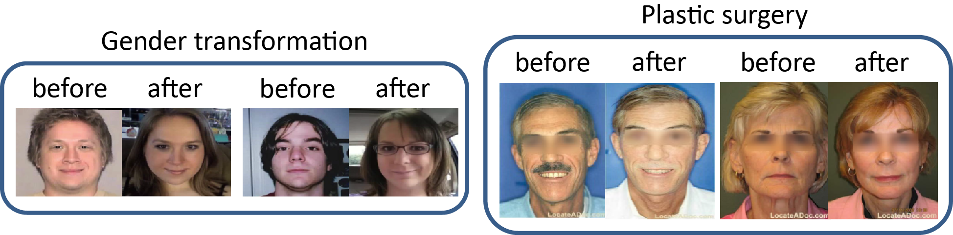
Fig. 4: Samples of subjects before/after undergoing gender transformation and plastic surgery. Images are from Mahalingam et al. (2014) and Jillela and Ross (2012).

Other studies are related with the effect on the recognition performance of plastic surgery or gender transformation, as presented in Section 6.3 (see Figure 4 as well). Mahalingam et al. (2014) studied the impact of gender transformation via Hormone Replacement Theory (HRT), which causes changes in the physical appearance of the face and body gradually over the course of the treatment. A database of $>$1.2 million face images from YouTube videos was built, with data from 38 subjects undergoing HRT over a period of several months to three years, observing that accuracy of the periocular region greatly outperformed other face components (nose, mouth) and the full face. Also, face matchers began to fail after only a few months of HRT treatment. Jillela and Ross (2012) studied the matching of face images before and after undergoing plastic surgery. The work proposed a fusion recognition approach that combines face and periocular information, outperforming previous studies where only full-face matchers were used.

8 Conclusions and future work

Periocular recognition has emerged as a promising trait for unconstrained biometrics after demands for increased robustness of face or iris systems, showing a surprisingly high discrimination ability (Santos and Proenca, 2013). The fast-growing uptake of face technologies in social networks and smartphones, as well as the widespread use of surveillance cameras, arguably increases the interest of periocular biometrics. The periocular region has shown to be more tolerant to variability in expression, occlusion, and it has more capability of matching partial faces (Juefei-Xu and Savvides, 2014). It also finds applicability in other areas such as forensics analysis (crime scene images where perpetrators intentionally mask part of their faces). In such situation, identifying a suspect where only the periocular region is visible is one of the toughest real-world challenges in biometrics. Even in this difficult case, the periocular region can aid in the reconstruction of the whole face (Juefei-Xu et al., 2014).

This paper reviews the state of the art in periocular biometrics research. Our target is to provide a comprehensive coverage of the existing literature, giving an insight of the most relevant issues and challenges. We start by presenting existing databases utilized in periocular research. Acquisition setups comprise digital cameras, webcams, videocameras, smartphones, or close-up iris sensors. A small number of databases contain video data of subjects walking through an acquisition portal, or in hallways or atria. There are databases for particular problems too, such as aging, plastic surgery effects, gender transformation effects, expression changes, or cross-spectral matching. However, the use of databases acquired with personal devices such as smartphones or tablets is limited, with recognition accuracy still some steps behind (Santos et al., 2014). The same can be said about surveillance cameras (Juefei-Xu and Savvides, 2012). New sensors are being proposed, such as Light Field Cameras, which capture multiple images at different focus in a single capture (Raghavendra et al., 2013; Raja et al., 2014), guaranteeing to have a good focused image. Since the periocular modality requires less constrained acquisition than other ocular or face modalities, it is likely that the research community will move towards exploring ocular recognition at a distance and on the move in more detail as compared to previous studies (Nigam et al., 2015).

Automatic detection and/of segmentation of the periocular region has been increasingly addressed as well, avoiding the need of segmenting the iris or detecting the full face first (Table 2). Recently, the use of eye corners as reference points to define the periocular ROI has been suggested, instead of the eye center, since eye corners are less sensitive to gaze variations and also appear in closed eyes (Padole and Proenca, 2012; Proenca and Briceno, 2014; Nie et al., 2014). We further review the features employed for periocular recognition, which comprises the majority of works in the literature. They can be classified into global and local approaches (Figure 3). Some works have also addressed the task of assessing if there are regions of the periocular area more useful than others for recognition purposes. This has been done both by asking to humans (Hollingsworth et al., 2012) and by using several machine algorithms (Smereka and Kumar, 2013; Alonso-Fernandez and Bigun, 2014), with both humans and machines agreeing in the usefulness of different parts. Automatic segmentation of periocular parts can aid in avoiding those which are non-useful, as well as other elements such as hair or glasses, that can also deteriorate the recognition performance, as shown by Proenca et al. (2014) in the first work which present an algorithm to segment components of the periocular region. Since the periocular area appears in face and iris images, comparison and fusion with these modalities has been also proposed, with a review of related works also given (Table 4). Fusion of multiple modalities using ocular data is a promising path forward that is receiving increasing attention (Nigam et al., 2015) due to unconstrained environments where switching between available modalities may be necessary (Alonso-Fernandez et al., 2010).

Soft-biometrics is another area where the periocular modality has found applicability, with periocular features showing accuracies comparable to these obtained by using the entire face for the tasks of gender and ethnicity classification (Table 5). The periocular modality is also shown to aid or outperform face matchers in case of undergoing plastic surgery or gender transformation. Another issues that are receiving increasing attention is cross-modality (Jillela and Ross, 2014), cross-spectral (Cao and Schmid, 2014; Sharma et al., 2014), hyper-spectral (Uzair et al., 2015) or cross-sensor (Santos et al., 2014) matching. The periocular modality also has the potential to allow ocular recognition at large stand-off distances (Cao and Schmid, 2014), with applications in surveillance. Samples captured with different sensors are to be matched if, for example, people is allowed to use their own smartphone or surveillance cameras, or when new or improved sensors have to co-exist with existing ones (cross-sensor), not to mention if the sensors work in different spectral range (cross-spectral). Iris images are traditionally acquired in NIR spectrum, whereas face images normally are captured with VW sensors. Exchange of biometric information between different law enforcement agencies worldwide also poses similar problems. These are examples of some scenarios where, if biometrics is extensively deployed, data acquired from heterogeneous sources will have to co-exist (Alonso-Fernandez et al., 2010). These issues are of high interest in new scenarios arising from the widespread use of biometric technologies and the availability of multiple sensors and vendor solutions. Another important direction therefore is to enable periocular heterogeneous data to work together (Nigam et al., 2015).

References

- Adams et al. (2010) Adams, J., Woodard, D., Dozier, G., Miller, P., Bryant, K., Glenn, G., 2010. Genetic-based type ii feature extraction for periocular biometric recognition: Less is more. Proc Intl Conf Pattern Recognition, ICPR , 205–208.