Abstract

We propose shifted inner-product similarity (SIPS), which is a novel yet very simple extension of the ordinary inner-product similarity (IPS) for neural-network based graph embedding (GE). In contrast to IPS, that is limited to approximating positive-definite (PD) similarities, SIPS goes beyond the limitation by introducing bias terms in IPS; we theoretically prove that SIPS is capable of approximating not only PD but also conditionally PD (CPD) similarities with many examples such as cosine similarity, negative Poincaré distance and negative Wasserstein distance. Since SIPS with sufficiently large neural networks learns a variety of similarities, SIPS alleviates the need for configuring the similarity function of GE. Approximation error rate is also evaluated, and experiments on two real-world datasets demonstrate that graph embedding using SIPS indeed outperforms existing methods.

1 INTRODUCTION

Graph embedding (GE) of relational data, such as texts, images, and videos, etc., now plays an indispensable role in machine learning. To name but a few, words and contexts in a corpus constitute relational data, and their vector representations obtained by skip-gram model (Mikolov et al., 2013a, ) and GloVe (Pennington et al.,, 2014) are often used in natural language processing. More classically, a similarity graph is constructed from data vectors, and nodes are embedded to a lower dimensional space where connected nodes are closer to each other (Cai et al.,, 2018).

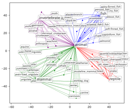
Figure 1: Visualization of word feature vectors for WordNet dataset computed by GE with our proposed SIPS model. See Supplement A for details.

Embedding is often designed so that the inner product between two vector representations in Euclidean space expresses their similarity. In addition to its interpretability, the inner product similarity has the following two desirable properties: (1) The vector representations are suitable for downstream tasks as feature vectors because machine learning methods are often based on inner products (e.g., kernel methods). (2) Simple vector arithmetic in the embedded space may represent similarity arithmetic such as the “linguistic regularities” of word vectors (Mikolov et al., 2013b, ). The latter property comes from the distributive law of inner product $\langle\boldsymbol{a}+\boldsymbol{b},\boldsymbol{c}\rangle=\langle\boldsymbol{a},\boldsymbol{c}\rangle+\langle\boldsymbol{b},\boldsymbol{c}\rangle$, which decomposes the similarity of $\boldsymbol{a}+\boldsymbol{b}$ and $\boldsymbol{c}$ into the sum of the two similarities. For seeking the word vector $\boldsymbol{y}^{\prime}=\boldsymbol{y}_{\text{queen}}$, we maximize $\langle\boldsymbol{y}_{\text{king}}-\boldsymbol{y}_{\text{man}}+\boldsymbol{y}_{\text{woman}},\boldsymbol{y}^{\prime}\rangle=\langle\boldsymbol{y}_{\text{king}},\boldsymbol{y}^{\prime}\rangle-\langle\boldsymbol{y}_{\text{man}},\boldsymbol{y}^{\prime}\rangle+\langle\boldsymbol{y}_{\text{woman}},\boldsymbol{y}^{\prime}\rangle$ in Eq. (3) of Levy and Goldberg, (2014). Thus solving analogy questions with vector arithmetic is mathematically equivalent to seeking a word which is similar to king and woman but is different from man.

Although classical GE has been quite successful, it considers simply the graph structure, where data vectors (pre-obtained attributes such as color-histograms of images), if any, are used only through the similarity graph. To fully utilize data vectors, neural networks (NNs) are incorporated into GE so that data vectors are converted to new vector representations (Kipf and Welling,, 2016; Zhanga et al.,, 2017; Hamilton et al.,, 2017; Dai et al.,, 2018), which reduces to the classical GE by taking 1-hot vectors as data vectors. While these methods consider $1$-view setting, multi-view setting is considered in Probabilistic Multi-view Graph Embedding (Okuno et al.,, 2018, PMvGE), which generalizes existing multivariate analysis methods (e.g., PCA and CCA) and NN-extensions (Andrew et al.,, 2013, DCCA) as well as graph embedding methods such as Locality Preserving Projections (He and Niyogi,, 2004; Yan et al.,, 2007, LPP), Cross-view Graph Embedding (Huang et al.,, 2012, CvGE), and Cross-Domain Matching Correlation Analysis (Shimodaira,, 2016, CDMCA). In these methods, the inner product of two vector representations obtained via NNs represents the strength of association between the corresponding two data vectors. The vector representations and the inner products are referred to as feature vectors and Inner Product Similarities (IPS), respectively, in this paper.

IPS is considered to be highly expressive for representing the association between data vectors due to the Universal Approximation Theorem (Funahashi,, 1989; Cybenko,, 1989; Yarotsky,, 2017; Telgarsky,, 2017, UAT) for NN, which proves that NNs having many hidden units approximate arbitrary continuous functions within any given accuracy. However, since IPS considers the inner product of two vector-valued NNs, the UAT is not directly applicable to the whole network with the constraints at the final layer. Thus the approximation capability of IPS is yet to be clarified.

For that reason, Okuno et al., (2018) incorporates UAT into Mercer’s theorem (Minh et al.,, 2006) and proves that IPS approximates any similarity based on Positive Definite (PD) kernels arbitrary well. For example, IPS can learn cosine similarity, because it is a PD kernel. This result shows not only the validity but also the fundamental limitation of IPS, meaning that the PD-ness of the kernels is required for IPS.

To overcome the limitation, similarities based on specific kernels other than the inner product have received considerable attention in recent years. One example is Poincaré embedding (Nickel and Kiela,, 2017) which is an NN-based GE using Poincaré distance for embedding vectors in hyperbolic space instead of Euclidean space. Hyperbolic space is especially compatible with computing feature vectors of tree-structured relational data (Sarkar,, 2011). While these methods efficiently compute reasonable low-dimensional feature vectors by virtue of specific kernels, their theoretical differences from IPS is not well understood.

In order to provide theoretical insights on these methods, in this paper, we will point out that some specific kernels are not PD by referring to existing studies. To deal with such non-PD kernels, we consider Conditionally PD (CPD) kernels (Berg et al.,, 1984; Schölkopf,, 2001) which include PD kernels as special cases. We then propose a novel model named Shifted IPS (SIPS) that approximates similarities based on CPD kernels within any given accuracy. Interestingly, negative Poincaré distance is already proved to be CPD (Faraut and Harzallah,, 1974) and it is not PD. So, similarities based on this kernel can be approximated by SIPS but not by IPS. Although we can think of a further generalization beyond CPD, this is only touched in Supplement E by defining inner product difference similarity (IPDS) model.

Our contribution is summarized as follows:

1. We show that IPS cannot approximate a non-PD kernel; we propose SIPS to go beyond the limitation, and prove that SIPS can approximate any CPD similarities arbitrary well.

2. We evaluate the error rate for SIPS to approximate CPD similarities, by incorporating neural networks such as multi-layer perceptron and deep neural networks.

3. We conduct numerical experiments on two real-world datasets, to show that graph embedding using SIPS outperforms recent graph embedding methods.

This paper is an extension of Okuno and Shimodaira, (2018) presented at ICML2018 workshop.

2 BACKGROUND

We work on an undirected graph consisting of $n$ nodes $\{v_{i}\}_{i=1}^{n}$ and link weights $\{w_{ij}\}_{i,j=1}^{n}\subset\mathbb{R}_{\geq 0}$ satisfying $w_{ij}=w_{ji}$ and $w_{ii}=0$, where $w_{ij}$ represents the strength of association between $v_{i}$ and $v_{j}$. The data vector representing the attributes (or side-information) at $v_{i}$ is denoted as $\boldsymbol{x}_{i}\in\mathbb{R}^{p}$. If we have no attributes, we use 1-hot vectors in $\mathbb{R}^{n}$ instead. We assume that the observed dataset consists of $\{w_{ij}\}_{i,j=1}^{n}$ and $\{\boldsymbol{x}_{i}\}_{i=1}^{n}$.

Let us consider a simple random graph model for the generative model of random variables $\{w_{ij}\}_{i,j=1}^{n}$ given data vectors $\{\boldsymbol{x}_{i}\}_{i=1}^{n}$. The conditional distribution of $w_{ij}$ is specified by a similarity function $h(\boldsymbol{x}_{i},\boldsymbol{x}_{j})$ of the two data vectors. Typically, Bernoulli distribution $P(w_{ij}=1|\boldsymbol{x}_{i},\boldsymbol{x}_{j})=\sigma(h(\boldsymbol{x}_{i},\boldsymbol{x}_{j}))$ with sigmoid function $\sigma(x):=(1+\exp(-x))^{-1}$ for 0-1 variable $w_{ij}\in\{0,1\}$, and Poisson distribution $w_{ij}\sim\text{Po}(\exp(h(\boldsymbol{x}_{i},\boldsymbol{x}_{j})))$ for non-negative integer variable $w_{ij}\in\{0,1,\ldots\}$ are used to model the conditional probability. These models are in fact specifying the conditional expectation $E(w_{ij}|\boldsymbol{x}_{i},\boldsymbol{x}_{j})$ by $\sigma(h(\boldsymbol{x}_{i},\boldsymbol{x}_{j}))$ and $\exp(h(\boldsymbol{x}_{i},\boldsymbol{x}_{j}))$, respectively, and they correspond to logistic regression and Poisson regression in the context of generalized linear models.

These two generative models are closely related. Let $w_{ij}\sim\text{Po}(\lambda_{ij})$ with $\lambda_{ij}=\exp(h(\boldsymbol{x}_{i},\boldsymbol{x}_{j}))$. Then Supplement B shows that

$$P(w_{ij}=1\mid\boldsymbol{x}_{i},\boldsymbol{x}_{j})=\sigma(h(\boldsymbol{x}_{i},\boldsymbol{x}_{j}))+O(\lambda_{ij}^{3})$$ (1)

and $P(w_{ij}\geq 2)=O(\lambda_{ij}^{2})$, indicating that, for sufficiently small $\lambda_{ij}$, the Poisson model is well approximated by the Bernoulli model. Since these two models are not very different in this sense, we consider only the Poisson model in this paper.

We write the similarity function as

$$h(\boldsymbol{x}_{i},\boldsymbol{x}_{j}):=g(\boldsymbol{f}(\boldsymbol{x}_{i}),\boldsymbol{f}(\boldsymbol{x}_{j})),$$ (2)

where $\boldsymbol{f}:\mathbb{R}^{p}\to\mathbb{R}^{K}$ is a continuous function and $g:\mathbb{R}^{K\times K}\to\mathbb{R}$ is a symmetric continuous function. For two data vectors $\boldsymbol{x}_{i}$ and $\boldsymbol{x}_{j}$, their feature vectors are defined as $\boldsymbol{y}_{i}=\boldsymbol{f}(\boldsymbol{x}_{i})$ and $\boldsymbol{y}_{j}=\boldsymbol{f}(\boldsymbol{x}_{j})$, thus the similarity function is also written as $g(\boldsymbol{y}_{i},\boldsymbol{y}_{j})$. In particular, we consider a vector-valued neural network (NN) $\boldsymbol{y}=\boldsymbol{f}_{\text{NN}}(\boldsymbol{x})$ for computing the feature vector, then $g(\boldsymbol{f}_{\text{NN}}(\boldsymbol{x}_{i}),\boldsymbol{f}_{\text{NN}}(\boldsymbol{x}_{j}))$ is especially called siamese network (Bromley et al.,, 1994) in neural network literature. The original form of siamese network uses the cosine similarity for $g$, but we can specify other types of similarity function. By specifying the inner product $g(\boldsymbol{y},\boldsymbol{y}^{\prime})=\langle\boldsymbol{y},\boldsymbol{y}^{\prime}\rangle$, the similarity function (2) becomes

$$h(\boldsymbol{x}_{i},\boldsymbol{x}_{j})=\langle\boldsymbol{f}_{\text{NN}}(\boldsymbol{x}_{i}),\boldsymbol{f}_{\text{NN}}(\boldsymbol{x}_{j})\rangle.$$ (3)

We call (3) as Inner Product Similarity (IPS) model. IPS commonly appears in a broad range of methods, such as DeepWalk (Perozzi et al.,, 2014), LINE (Tang et al.,, 2015), node2vec (Grover and Leskovec,, 2016), Variational Graph AutoEncoder (Kipf and Welling,, 2016), and GraphSAGE (Hamilton et al.,, 2017). Multi-view extensions (Okuno et al.,, 2018) with views $d=1,\ldots,D$, are easily obtained by preparing a neural network $\boldsymbol{f}_{\text{NN}}^{(d)}$ for each view.

3 PD SIMILARITIES

In order to prove the approximation capability of IPS given in eq. (3), Okuno et al., (2018) incorporates the UAT for NN (Funahashi,, 1989; Cybenko,, 1989; Yarotsky,, 2017; Telgarsky,, 2017) into Mercer’s theorem (Minh et al.,, 2006). In this section, we review their assertion that shows uniform convergence of IPS to any PD similarity. To show the result in Theorem 3.2, we first define a kernel and its positive-definiteness.

Definition 3.1

For some set $\mathcal{Y}$, a symmetric continuous function $g:\mathcal{Y}^{2}\to\mathbb{R}$ is called a kernel on $\mathcal{Y}^{2}$.

Definition 3.2

A kernel $g$ on $\mathcal{Y}^{2}$ is said to be Positive Definite (PD) if satisfying $\sum_{i=1}^{n}\sum_{j=1}^{n}c_{i}c_{j}g(\boldsymbol{y}_{i},\boldsymbol{y}_{j})\geq 0$ for arbitrary $c_{1},c_{2},\ldots,c_{n}\in\mathbb{R},\boldsymbol{y}_{1},\boldsymbol{y}_{2},\ldots,\boldsymbol{y}_{n}\in\mathcal{Y}$.

For instance, cosine similarity $g(\boldsymbol{y},\boldsymbol{y}^{\prime}):=\langle\frac{\boldsymbol{y}}{\|\boldsymbol{y}\|_{2}},\frac{\boldsymbol{y}^{\prime}}{\|\boldsymbol{y}^{\prime}\|_{2}}\rangle$ is a PD kernel on $(\mathbb{R}^{p}\setminus\{\boldsymbol{0}\})^{2}$. Its PD-ness immediately follows from $\sum_{i=1}^{n}\sum_{j=c}^{n}c_{i}c_{j}g(\boldsymbol{y}_{i},\boldsymbol{y}_{j})=\|\sum_{i=1}^{n}c_{i}\frac{\boldsymbol{y}_{i}}{\|\boldsymbol{y}_{i}\|_{2}}\|_{2}^{2}\geq 0$ for arbitrary $\{c_{i}\}_{i=1}^{n}\subset\mathbb{R}$ and $\{\boldsymbol{y}_{i}\}_{i=1}^{n}\subset\mathcal{Y}$. Also polynomial kernel, Gaussian kernel, and Laplacian kernel are PD (Berg et al.,, 1984).

Definition 3.3

A function $h(\boldsymbol{x},\boldsymbol{x}^{\prime}):=g(\boldsymbol{f}(\boldsymbol{x}),\boldsymbol{f}(\boldsymbol{x}^{\prime}))$ with a continuous function $\boldsymbol{f}:\mathcal{X}\to\mathcal{Y}$ and a kernel $g:\mathcal{Y}^{2}\to\mathbb{R}$ is called a similarity on $\mathcal{X}^{2}$.

For a PD kernel $g$, the similarity $h$ is also a PD kernel on $\mathcal{X}^{2}$, since $\sum_{i=1}^{n}\sum_{j=1}^{n}c_{i}c_{j}h(\boldsymbol{x}_{i},\boldsymbol{x}_{j})=\sum_{i=1}^{n}\sum_{j=1}^{n}c_{i}c_{j}g(\boldsymbol{f}(\boldsymbol{x}_{i}),\boldsymbol{f}(\boldsymbol{x}_{j}))\geq 0$.

Briefly speaking, a similarity $h$ is used for measuring how similar two data vectors are, while a kernel $g$ is used to compare feature vectors.

The following theorem (Minh et al.,, 2006) shows existence of a series expansion of any PD kernel, which has been utilized in kernel methods in machine learning (Hofmann et al.,, 2008).

Theorem 3.1 (Mercer’s theorem)

For some compact set $\mathcal{Y}\subset\mathbb{R}^{K^{*}}$, $K^{*}\in\mathbb{N}$, we consider a positive definite kernel $g_{*}:\mathcal{Y}^{2}\to\mathbb{R}$. Then, there exist nonnegative eigenvalues $\{\lambda_{k}\}_{k=1}^{\infty}$, $\lambda_{1}\geq\lambda_{2}\geq\cdots$, and continuous eigenfunctions $\{\phi_{k}\}_{k=1}^{\infty}$ such that

$$g_{*}(\boldsymbol{y}_{*},\boldsymbol{y}_{*}^{\prime})=\sum_{k=1}^{\infty}\lambda_{k}\phi_{k}(\boldsymbol{y}_{*})\phi_{k}(\boldsymbol{y}_{*}^{\prime}),$$ (4)

for all $\boldsymbol{y}_{*},\boldsymbol{y}_{*}^{\prime}\in\mathcal{Y}$, where the series convergences absolutely for each $(\boldsymbol{y}_{*},\boldsymbol{y}_{*}^{\prime})$ and uniformly for $\mathcal{Y}$.

Note that the condition (2) in Minh et al., (2006), i.e., $\int_{\mathcal{Y}}\int_{\mathcal{Y}}g_{*}(\boldsymbol{y}_{*},\boldsymbol{y}_{*}^{\prime})\,d\boldsymbol{y}_{*}\,d\boldsymbol{y}_{*}^{\prime}<\infty$, holds since $g_{*}$ is continuous and $\mathcal{Y}$ is compact. The theorem can be extended to closed set $\mathcal{Y}$, but we assume compactness for simplifying our argument.

It is obvious that IPS is always PD, because $\sum_{i=1}^{n}\sum_{j=1}^{n}c_{i}c_{j}\big{\langle}\boldsymbol{f}_{\text{NN}}(\boldsymbol{x}_{i}),\boldsymbol{f}_{\text{NN}}(\boldsymbol{x}_{j})\big{\rangle}=\|\sum_{i=1}^{n}c_{i}\boldsymbol{f}_{\text{NN}}(\boldsymbol{x}_{i})\|_{2}^{2}\geq 0$. We would like to show the converse: IPS approximates any PD similarities. This is given by the Approximation Theorem (AT) for IPS below, which is Theorem 5.1 $(D=1)$ of Okuno et al., (2018). The idea is to incorporate the UAT for NN into Mercer’s theorem (Theorem 3.1).

Theorem 3.2 (AT for IPS)

For $\mathcal{X}=[-M,M]^{p}$, $M>0$, and some compact set $\mathcal{Y}\subset\mathbb{R}^{K^{*}}$, $K^{*}\in\mathbb{N}$, we consider a continuous function $\boldsymbol{f}_{*}:\mathcal{X}\to\mathcal{Y}$ and a PD kernel $g^{\text{(PD)}}_{*}:\mathcal{Y}^{2}\to\mathbb{R}$. Let $\sigma(\cdot)$ be ReLU or an activation function which is non-constant, continuous, bounded, and monotonically-increasing. Then, for arbitrary $\varepsilon>0$, by specifying sufficiently large $K\in\mathbb{N},m_{f}=m_{f}(K)\in\mathbb{N}$, there exist $\boldsymbol{A}\in\mathbb{R}^{K\times m_{f}},\boldsymbol{B}\in\mathbb{R}^{m_{f}\times p},\boldsymbol{c}\in\mathbb{R}^{m_{f}}$ such that

for all $(\boldsymbol{x},\boldsymbol{x}^{\prime})\in\mathcal{X}^{2}$, where $\boldsymbol{f}_{\text{NN}}(\boldsymbol{x})=\boldsymbol{A}\boldsymbol{\sigma}(\boldsymbol{B}\boldsymbol{x}+\boldsymbol{c})$ is a $1$-hidden layer neural network with $m_{f}$ hidden units and $K$ outputs, and $\boldsymbol{\sigma}(\boldsymbol{x})$ is element-wise $\sigma(\cdot)$ function.

See Supplement A of Okuno et al., (2018) for the proof. It is based on the series expansion $g^{\text{(PD)}}_{*}(\boldsymbol{y}_{*},\boldsymbol{y}_{*}^{\prime})=\sum_{k=1}^{\infty}\lambda_{k}\phi_{k}(\boldsymbol{y}_{*})\phi_{k}(\boldsymbol{y}_{*}^{\prime})$ of Mercer’s theorem (Theorem 3.1) for arbitrary PD kernel $g^{\text{(PD)}}_{*}$. This expansion indicates with a vector-valued function $\tilde{\boldsymbol{\phi}}_{K}(\boldsymbol{x}):=(\lambda_{1}^{1/2}\phi_{1}(\boldsymbol{f}_{*}(\boldsymbol{x})),\ldots,\lambda_{K}^{1/2}\phi_{K}(\boldsymbol{f}_{*}(\boldsymbol{x})))$ that

$$\langle\tilde{\boldsymbol{\phi}}_{K}(\boldsymbol{x}),\tilde{\boldsymbol{\phi}}_{K}(\boldsymbol{x}^{\prime})\rangle\to g^{\text{(PD)}}_{*}(\boldsymbol{f}_{*}(\boldsymbol{x}),\boldsymbol{f}_{*}(\boldsymbol{x}^{\prime})),\>K\to\infty,$$

for all $\boldsymbol{x},\boldsymbol{x}^{\prime}$. Considering a vector-valued NN $\boldsymbol{f}_{\text{NN}}:\mathbb{R}^{p}\to\mathbb{R}^{K}$ that approximates $\tilde{\boldsymbol{\phi}}_{K}$, the IPS $\langle\boldsymbol{f}_{\text{NN}}(\boldsymbol{x}),\boldsymbol{f}_{\text{NN}}(\boldsymbol{x}^{\prime})\rangle\approx\langle\tilde{\boldsymbol{\phi}}_{K}(\boldsymbol{x}),\tilde{\boldsymbol{\phi}}_{K}(\boldsymbol{x}^{\prime})\rangle$ converges to $g^{\text{(PD)}}_{*}(\boldsymbol{f}_{*}(\boldsymbol{x}),\boldsymbol{f}_{*}(\boldsymbol{x}^{\prime}))$ as $K\to\infty$, thus proving the assertion. In addition to the uniform convergence shown in Theorem 3.2, the approximation error rate will be evaluated in Section 5.

Unlike Mercer’s theorem which indicates only the existence of the feature map $\tilde{\boldsymbol{\phi}}_{K}$, Theorem 3.2 shows that a neural network $\boldsymbol{f}_{\text{NN}}:\mathbb{R}^{p}\to\mathbb{R}^{K}$ can be implemented so that the IPS $\langle\boldsymbol{f}_{\text{NN}}(\boldsymbol{x}),\boldsymbol{f}_{\text{NN}}(\boldsymbol{x}^{\prime})\rangle$ eventually approximates the PD similarity $g^{\text{(PD)}}_{*}(\boldsymbol{f}_{*}(\boldsymbol{x}),\boldsymbol{f}_{*}(\boldsymbol{x}^{\prime}))$ arbitrary well.

Note that Theorem 3.2 is AT for IPS which shows only the existence of NNs with required accuracy. Although we do not go further in this paper, consistency of the maximum likelihood estimation implemented as SGD is discussed in Section 5.2 and Supplement B of Okuno et al., (2018) for showing that IPS actually learns any PD similarities by increasing $n$.

4 CPD SIMILARITIES

Theorem 3.2 shows that IPS approximates any PD similarities arbitrary well. However, similarities in general are not always PD. To deal with non-PD similarities, we consider a class of similarities based on Conditionally PD (CPD) kernels (Berg et al.,, 1984; Schölkopf,, 2001) which includes PD kernels as special cases. We then extend IPS to approximate CPD similarities.

Someone may wonder why only similarities based on inner product are considered in this paper. In fact, it is obvious that a real-valued NN $f_{\text{NN}}(\boldsymbol{x},\boldsymbol{x}^{\prime})$ with sufficiently many hidden units approximates any similarity $h(\boldsymbol{x},\boldsymbol{x}^{\prime})$ arbitrary well. This is an immediate consequence of the UAT directly applied to $f_{\text{NN}}(\boldsymbol{x},\boldsymbol{x}^{\prime})$. Therefore, considering the form $\langle\boldsymbol{f}_{\text{NN}}(\boldsymbol{x}),\boldsymbol{f}_{\text{NN}}(\boldsymbol{x}^{\prime})\rangle$ or its extension just makes the problem harder. Our motivation in this paper is that we would like to utilize the feature vector $\boldsymbol{y}=\boldsymbol{f}_{\text{NN}}(\boldsymbol{x})$ with nice properties such as “linguistic regularities” which may follow from the constraint of the inner product.

The remaining of this section is organized as follows. In Section 4.1, we point out the fundamental limitation of IPS to approximate a non-PD similarity. In Section 4.2, we define CPD kernels with some examples. In Section 4.3, we propose a novel Shifted IPS (SIPS), by extending the IPS. In Section 4.4, we give interpretations of SIPS and its simpler variant C-SIPS. In Section 4.5, we prove that SIPS approximates CPD similarities arbitrary well.

4.1 Fundamental Limitation of IPS

Let us consider the negative squared distance (NSD) $g(\boldsymbol{y},\boldsymbol{y}^{\prime})=-\|\boldsymbol{y}-\boldsymbol{y}^{\prime}\|_{2}^{2}$ and the identity map $\boldsymbol{f}(\boldsymbol{x})=\boldsymbol{x}$. Then the similarity function

$$h(\boldsymbol{x},\boldsymbol{x}^{\prime})=g(\boldsymbol{f}(\boldsymbol{x}),\boldsymbol{f}(\boldsymbol{x}^{\prime}))=-\|\boldsymbol{x}-\boldsymbol{x}^{\prime}\|_{2}^{2}$$

defined on $\mathbb{R}^{p}\times\mathbb{R}^{p}$ is not PD but CPD, which is defined later in Section 4.2. Regarding the NSD similarity, Proposition 4.1 shows a strictly positive lower bound of approximation error for IPS.

Proposition 4.1

For all $M>0,p,K\in\mathbb{N}$, and a set of all $\mathbb{R}^{K}$-valued continuous functions $\mathfrak{S}(K)$, we have

$$\inf_{\boldsymbol{f}\in\mathfrak{S}(K)}\frac{1}{(2M)^{2p}}\int_{[-M,M]^{p}}\int_{[-M,M]^{p}}$$

$$\hskip 20.00003pt\bigg{|}-\|\boldsymbol{x}-\boldsymbol{x}^{\prime}\|_{2}^{2}-\langle\boldsymbol{f}(\boldsymbol{x}),\boldsymbol{f}(\boldsymbol{x}^{\prime})\rangle\bigg{|}\mathrm{d}\boldsymbol{x}\mathrm{d}\boldsymbol{x}^{\prime}\geq\frac{2pM^{2}}{3}.$$

The proof is given in Supplement C.1.

Since $\mathfrak{S}(K)$ includes neural networks, Proposition 4.1 indicates that IPS does not approximate NSD similarity arbitrary well, even if NN has a huge amount of hidden units with sufficiently large output dimension.

4.2 CPD Kernels and Similarities

Here, we introduce similarities based on Conditionally PD (CPD) kernels (Berg et al.,, 1984; Schölkopf,, 2001) in order to consider non-PD similarities which IPS does not approximate arbitrary well. We first define CPD kernels.

Definition 4.1

A kernel $g$ on $\mathcal{Y}^{2}$ is called Conditionally PD (CPD) if $\sum_{i=1}^{n}\sum_{j=1}^{n}c_{i}c_{j}g(\boldsymbol{y}_{i},\boldsymbol{y}_{j})\geq 0$ holds for arbitrary $c_{1},c_{2},\ldots,c_{n}\in\mathbb{R},\boldsymbol{y}_{1},\boldsymbol{y}_{2},\ldots,\boldsymbol{y}_{n}\in\mathcal{Y}$ with the constraint $\sum_{i=1}^{n}c_{i}=0$.

The difference between the definitions of CPD and PD kernels is whether it imposes the constraint $\sum_{i=1}^{n}c_{i}=0$ or not. According to these definitions, CPD kernels include PD kernels as special cases. For a CPD kernel $g$, the similarity $h$ is also a CPD kernel on $\mathcal{X}^{2}$.

A simple example of CPD kernel is $g(\boldsymbol{y},\boldsymbol{y}^{\prime})=-\|\boldsymbol{y}-\boldsymbol{y}^{\prime}\|_{2}^{\alpha}$ for $0<\alpha\leq 2$ defined on $\mathbb{R}^{K}\times\mathbb{R}^{K}$. Other examples are $-(\sin(y-y^{\prime}))^{2}$ and $-\boldsymbol{1}_{(0,\infty)}(y+y^{\prime})$ on $\mathbb{R}\times\mathbb{R}$. CPD-ness is a well-established concept with interesting properties (Berg et al.,, 1984): For any function $u(\cdot)$, $g(\boldsymbol{y},\boldsymbol{y}^{\prime})=u(\boldsymbol{y})+u(\boldsymbol{y}^{\prime})$ is CPD. Constants are CPD. The sum of two CPD kernels is also CPD. For CPD kernels $g$ with $g(\boldsymbol{y},\boldsymbol{y}^{\prime})\leq 0$, CPD-ness holds for $-(-g)^{\alpha}\>(\alpha\in(0,1])$ and $-\log(1-g)$.

Example 4.1 (Poincaré distance)

For open unit ball $B^{K}:=\{\boldsymbol{y}\in\mathbb{R}^{K}\mid\|\boldsymbol{y}\|_{2}<1\}$, we define a distance between $\boldsymbol{y},\boldsymbol{y}^{\prime}\in B^{K}$ as

where $\cosh^{-1}(z)=\log(z+\sqrt{z^{2}-1})$. Considering the generative model of Section 2 with 1-hot data vectors, Poincaré embedding (Nickel and Kiela,, 2017) learns parameters $\boldsymbol{y}_{i}$, $i=1,\ldots,n$, by fitting $\sigma(-d_{\text{Poincar\'{e}}}(\boldsymbol{y}_{i},\boldsymbol{y}_{j}))$ to the observed $w_{ij}\in\{0,1\}$. Lorentz embedding (Nickel and Kiela,, 2018) reformulate Poincaré embedding with a specific variable transformation, that enables more efficient computation.

Interestingly, negative Poincaré distance is proved to be CPD in Faraut and Harzallah, (1974, Corollary 7.4).

Proposition 4.2

$-d_{\text{Poincar\'{e}}}$ is CPD on $B^{K}\times B^{K}$.

$-d_{\text{Poincar\'{e}}}$ is strictly CPD in the sense that $-d_{\text{Poincar\'{e}}}$ is not PD. A counter-example of PD-ness is, for example, $n=2,K=2,c_{1}=c_{2}=1,\boldsymbol{y}_{1}=(1/2,1/2),\boldsymbol{y}_{2}=(0,0)\in B^{2}$.

Another interesting example of CPD kernels is negative Wasserstein distance.

Example 4.2 (Wasserstein distance)

Let $\boldsymbol{Z}$ be a metric space endowed with a metric $d_{Z}$, which we call as “ground distance”. For $q\geq 1$, let $\mathcal{Y}$ be the space of all measures $\mu$ on $\boldsymbol{Z}$ satisfying $\int_{\boldsymbol{Z}}d_{Z}(\boldsymbol{z},\boldsymbol{z}_{0})^{q}\mathrm{d}\mu(\boldsymbol{z})<\infty$ for some $\boldsymbol{z}_{0}\in\boldsymbol{Z}$. The $q$-Wasserstein distance between $\boldsymbol{y},\boldsymbol{y}^{\prime}\in\mathcal{Y}$ is defined as

$$\scalebox{0.9}{$\displaystyle d_{W}^{(q)}(\boldsymbol{y},\boldsymbol{y}^{\prime}):=\left(\inf_{\pi\in\Pi(\boldsymbol{y},\boldsymbol{y}^{\prime})}\iint_{\boldsymbol{Z}\times\boldsymbol{Z}}d_{Z}(\boldsymbol{z},\boldsymbol{z}^{\prime})^{q}\mathrm{d}\pi(\boldsymbol{z},\boldsymbol{z}^{\prime})\right)^{1/q}$}.$$

Here, $\Pi(\boldsymbol{y},\boldsymbol{y}^{\prime})$ is the set of joint probability measures on $\boldsymbol{Z}\times\boldsymbol{Z}$ having marginals $\boldsymbol{y},\boldsymbol{y}^{\prime}$. Wasserstein distance is used for a broad range of methods, such as Generative Adversarial Networks (Arjovsky et al.,, 2017) and AutoEncoder (Tolstikhin et al.,, 2018).

Some cases of negative Wasserstein distance are proved to be CPD.

Proposition 4.3

$-d_{W}^{(1)}$ is CPD on $\mathcal{Y}^{2}$ if $-d_{Z}$ is CPD on $\boldsymbol{Z}^{2}$. $-d_{W}^{(2)}$ is CPD on $\mathcal{Y}^{2}$ if $\boldsymbol{Z}$ is a subset of $\mathbb{R}$.

$-d_{W}^{(1)}$ is known as the negative earth mover’s distance, and its CPD-ness is discussed in Gardner et al., (2017). The CPD-ness of a special case of $-d_{W}^{(2)}$ is shown in Kolouri et al., (2016) Corollary 1. However, we note that negative Wasserstein distance, in general, is not necessarily CPD. As Proposition 4.3 states, $\boldsymbol{Z}$ is required to be a subset of $\mathbb{R}$ when considering $q>1$.

4.3 Proposed Models

For approximating CPD similarities, we propose a novel similarity model

$$h(\boldsymbol{x}_{i},\boldsymbol{x}_{j}) =\langle\boldsymbol{f}_{\text{NN}}(\boldsymbol{x}_{i}),\boldsymbol{f}_{\text{NN}}(\boldsymbol{x}_{j})\rangle$$

$$\hskip 60.00009pt+u_{\text{NN}}(\boldsymbol{x}_{i})+u_{\text{NN}}(\boldsymbol{x}_{j}),$$ (6)

where $\boldsymbol{f}_{\text{NN}}:\mathbb{R}^{p}\to\mathbb{R}^{K}$ and $u_{\text{NN}}:\mathbb{R}^{p}\to\mathbb{R}$ are vector-valued and real-valued NNs, respectively. We call (6) as Shifted IPS (SIPS) model, because the IPS $\langle\boldsymbol{f}_{\text{NN}}(\boldsymbol{x}_{i}),\boldsymbol{f}_{\text{NN}}(\boldsymbol{x}_{j})\rangle$ given in (3) is shifted by the offset $u_{\text{NN}}(\boldsymbol{x}_{i})+u_{\text{NN}}(\boldsymbol{x}_{j})$. For illustrating how SIPS expresses CPD similarities, let us consider the NSD discussed in Section 4.1:

$$-\|\boldsymbol{x}_{i}-\boldsymbol{x}_{j}\|_{2}^{2}=\langle\sqrt{2}\boldsymbol{x}_{i},\sqrt{2}\boldsymbol{x}_{j}\rangle-\|\boldsymbol{x}_{i}\|_{2}^{2}-\|\boldsymbol{x}_{j}\|_{2}^{2}$$

is expressed by SIPS with $\boldsymbol{f}_{\text{NN}}(\boldsymbol{x})=\sqrt{2}\boldsymbol{x}$ and $u_{\text{NN}}(\boldsymbol{x})=-\|\boldsymbol{x}\|_{2}^{2}$. Later, we show in Theorem 4.1 that SIPS approximates any CPD similarities arbitrary well.

We also consider a simplified version of SIPS. By assuming $u_{\text{NN}}(\boldsymbol{x})=-\gamma/2$ for all $\boldsymbol{x}$, SIPS reduces to

$$h(\boldsymbol{x}_{i},\boldsymbol{x}_{j})=\langle\boldsymbol{f}_{\text{NN}}(\boldsymbol{x}_{i}),\boldsymbol{f}_{\text{NN}}(\boldsymbol{x}_{j})\rangle-\gamma,$$ (7)

where $\gamma\in\mathbb{R}$ is a parameter to be estimated. We call (7) as Constantly-Shifted IPS (C-SIPS) model.

If we have no attributes, we use 1-hot vectors for $\boldsymbol{x}_{i}$ in $\mathbb{R}^{n}$ instead, and $\boldsymbol{f}_{\text{NN}}(\boldsymbol{x}_{i})={\boldsymbol{y}}_{i}\in\mathbb{R}^{K}$, $u_{\text{NN}}(\boldsymbol{x}_{i})=u_{i}\in\mathbb{R}$ are model parameters. Then SIPS reduces to the matrix decomposition model with biases

$$h(\boldsymbol{x}_{i},\boldsymbol{x}_{j})=\langle{\boldsymbol{y}}_{i},{\boldsymbol{y}}_{j}\rangle+u_{i}+u_{j}.$$ (8)

This model is widely used for recommender systems (Koren et al.,, 2009) and word embedding such as GloVe (Pennington et al.,, 2014), and SIPS is considered as its generalization.

4.4 Interpretation of SIPS and C-SIPS

Here we illustrate the interpretation of the proposed models by returning back to the setting in Section 2. We consider a simple generative model of independent Poisson distribution with mean parameter $E(w_{ij})=\exp(h(\boldsymbol{x}_{i},\boldsymbol{x}_{j}))$. Then SIPS gives a generative model

(9)

where $\beta(\boldsymbol{x}):=\exp(u_{\text{NN}}(\boldsymbol{x}))>0$. Since $\beta(\boldsymbol{x})$ can be regarded as the “importance weight” of data vector $\boldsymbol{x}$, SIPS naturally incorporates the weight function $\beta(\boldsymbol{x})$ to probabilistic models used in a broad range of existing methods. Similarly, C-SIPS gives a generative model

$$w_{ij}\overset{\text{indep.}}{\sim}\text{Po}\Bigl{(}\alpha\exp(\langle\boldsymbol{f}_{\text{NN}}(\boldsymbol{x}_{i}),\boldsymbol{f}_{\text{NN}}(\boldsymbol{x}_{j})\rangle)\Bigr{)},$$ (10)

where $\alpha:=\exp(-\gamma)>0$ regulates the sparseness of $\{w_{ij}\}$. The generative model (10) is already proposed as 1-view PMvGE (Okuno et al.,, 2018).

It was shown in Supplement C of Okuno et al., (2018) that PMvGE (based on C-SIPS) approximates CDMCA when $w_{ij}$ is replaced by $\delta_{ij}$ in the constraint (8) therein, and this result can be extended so that PMvGE with SIPS approximates the original CDMCA using $w_{ij}$ in the constraint.

4.5 Approximation Theorems

It is obvious that SIPS is always CPD, because $\sum_{i=1}^{n}\sum_{j=1}^{n}c_{i}c_{j}\big{(}\langle\boldsymbol{f}_{\text{NN}}(\boldsymbol{x}_{i}),\boldsymbol{f}_{\text{NN}}(\boldsymbol{x}_{j})\rangle+u_{\text{NN}}(\boldsymbol{x}_{i})+u_{\text{NN}}(\boldsymbol{x}_{j})\big{)}=\|\sum_{i=1}^{n}c_{i}\boldsymbol{f}_{\text{NN}}(\boldsymbol{x}_{i})\|_{2}^{2}+2(\sum_{i=1}c_{i})(\sum_{j=1}c_{j}u_{\text{NN}}(\boldsymbol{x}_{j}))\geq 0$ for any $c_{i}$’s with $\sum_{i=1}^{n}c_{i}=0$. We would like to show the converse: SIPS approximates any CPD similarities, and thus it overcomes the fundamental limitation of IPS. This is given in Theorem 4.1 below, by extending Theorem 3.2 of IPS to SIPS. Theorem 4.2 also proves that C-SIPS given in eq. (7) approximates CPD similarities in a weaker sense.

Theorem 4.1 (AT for SIPS)

For $\mathcal{X}=[-M,M]^{p}$, $M>0$, and some compact set $\mathcal{Y}\subset\mathbb{R}^{K^{*}}$, $K^{*}\in\mathbb{N}$, we consider a continuous function $\boldsymbol{f}_{*}:\mathcal{X}\to\mathcal{Y}$ and a CPD kernel $g^{\text{(CPD)}}_{*}:\mathcal{Y}^{2}\to\mathbb{R}$. Let $\sigma(\cdot)$ be ReLU or an activation function which is non-constant, continuous, bounded, and monotonically-increasing. Then, for arbitrary $\varepsilon>0$, by specifying sufficiently large $K\in\mathbb{N},m_{f}=m_{f}(K)\in\mathbb{N},m_{u}\in\mathbb{N}$, there exist $\boldsymbol{A}\in\mathbb{R}^{K\times m_{f}},\boldsymbol{B}\in\mathbb{R}^{m_{f}\times p},\boldsymbol{c}\in\mathbb{R}^{m_{f}},\boldsymbol{e}\in\mathbb{R}^{m_{u}},\boldsymbol{F}\in\mathbb{R}^{m_{u}\times p},\boldsymbol{o}\in\mathbb{R}^{m_{u}}$ such that

for all $(\boldsymbol{x},\boldsymbol{x}^{\prime})\in\mathcal{X}^{2}$, where $\boldsymbol{f}_{\text{NN}}(\boldsymbol{x})=\boldsymbol{A}\boldsymbol{\sigma}(\boldsymbol{B}\boldsymbol{x}+\boldsymbol{c})\in\mathbb{R}^{K}$ and $u_{\text{NN}}(\boldsymbol{x})=\langle\boldsymbol{e},\boldsymbol{\sigma}(\boldsymbol{F}\boldsymbol{x}+\boldsymbol{o})\rangle\in\mathbb{R}$ are one-hidden layer neural networks with $m_{f}$ and $m_{u}$ hidden units, respectively, and $\boldsymbol{\sigma}(\boldsymbol{x})$ is element-wise $\sigma(\cdot)$ function.

The proof is in Supplement C.2. It stands on Lemma 2.1 in Berg et al., (1984), which shows the equivalence of CPD-ness of $g^{\text{(CPD)}}_{*}(\boldsymbol{y},\boldsymbol{y}^{\prime})$ and PD-ness of

$$g_{0}(\boldsymbol{y},\boldsymbol{y}^{\prime}):= g_{*}^{\text{(CPD)}}(\boldsymbol{y},\boldsymbol{y}^{\prime})+g_{*}^{\text{(CPD)}}(\boldsymbol{y}_{0},\boldsymbol{y}_{0})$$

$$\quad-g_{*}^{\text{(CPD)}}(\boldsymbol{y},\boldsymbol{y}_{0})-g_{*}^{\text{(CPD)}}(\boldsymbol{y}^{\prime},\boldsymbol{y}_{0})$$ (11)

for any fixed $\boldsymbol{y}_{0}\in\mathcal{Y}$. Using $g_{0}$ and $h_{*}(\boldsymbol{x}):=g_{*}^{\text{(CPD)}}(\boldsymbol{f}_{*}(\boldsymbol{x}),\boldsymbol{y}_{0})-\frac{1}{2}g_{*}^{\text{(CPD)}}(\boldsymbol{y}_{0},\boldsymbol{y}_{0})$, we write

$$g^{\text{(CPD)}}_{*}(\boldsymbol{f}_{*}(\boldsymbol{x}),\boldsymbol{f}_{*}(\boldsymbol{x}^{\prime}))$$

$$\quad=g_{0}(\boldsymbol{f}_{*}(\boldsymbol{x}),\boldsymbol{f}_{*}(\boldsymbol{x}^{\prime}))+h_{*}(\boldsymbol{x})+h_{*}(\boldsymbol{x}^{\prime}).$$ (12)

AT for IPS shows that $\langle\boldsymbol{f}_{\text{NN}}(\boldsymbol{x}),\boldsymbol{f}_{\text{NN}}(\boldsymbol{x}^{\prime})\rangle$ approximates $g_{0}(\boldsymbol{f}_{*}(\boldsymbol{x}),\boldsymbol{f}_{*}(\boldsymbol{x}^{\prime}))$ arbitrary well, and UAT for NN shows that $u_{\text{NN}}(\boldsymbol{x})$ approximates $h_{*}(\boldsymbol{x})$ arbitrary well, thus proving the theorem.

Theorem 4.2 (AT for C-SIPS)

Symbols and assumptions are the same as those of Theorem 4.1. For arbitrary $\varepsilon>0$, by specifying sufficiently large $K\in\mathbb{N}$, $m_{f}=m_{f}(K)\in\mathbb{N}$, $r>0$, there exist $\boldsymbol{A}\in\mathbb{R}^{K\times m_{f}}$, $\boldsymbol{B}\in\mathbb{R}^{m_{f}\times p}$, $\boldsymbol{c}\in\mathbb{R}^{m_{f}}$, $\gamma=O(r^{2})$ such that

for all $(\boldsymbol{x},\boldsymbol{x}^{\prime})\in\mathcal{X}^{2}$, where $\boldsymbol{f}_{\text{NN}}(\boldsymbol{x})=\boldsymbol{A}\boldsymbol{\sigma}(\boldsymbol{B}\boldsymbol{x}+\boldsymbol{c})\in\mathbb{R}^{K}$ is a one-hidden layer neural network with $m_{f}$ hidden units.

The proof is in Supplement C.3.

There is an additional error term of $O(r^{-2})$ in Theorem 4.2. A large $r$ will reduce the error, but then large $\gamma=O(r^{2})$ value may lead to unstable computation for finding an optimal NN. Conversely, a small $r$ increases the upper bound of the approximation error . Thus, if available, we prefer SIPS in terms of both computational stability and small approximation error.

5 APPROXIMATION ERROR RATE

Thus far, we showed universal approximation capabilities of IPS and SIPS in Theorems 3.2 and 4.1. In this section, we evaluate error rates for these approximation theorems, by assuming some additional conditions. They are used for employing the theorems for eigenvalue decay rate of PD kernels (Cobos and Kühn,, 1990, Theorem 4) and approximation error rate for NNs (Yarotsky,, 2018).

Conditions on the similarity function: We consider the following conditions on the function $\boldsymbol{f}_{*}$ and the kernel $g_{*}$ for the underlying true similarity $g_{*}(\boldsymbol{f}(\boldsymbol{x}),\boldsymbol{f}(\boldsymbol{x}^{\prime}))$.

1. Eigenfunctions $\{\phi_{k}(\boldsymbol{y})\}_{k=1}^{\infty}$ of $g_{*}(\boldsymbol{y},\boldsymbol{y}^{\prime})$ defined in Theorem 3.1 are continuously differentiable, i.e., $C^{1}$, and uniformly bounded in the sense of $\displaystyle\sup_{k\in\mathbb{N},\boldsymbol{y}\in\mathcal{Y}}|\phi_{k}(\boldsymbol{y})|<\infty$ and $\displaystyle\sup_{k\in\mathbb{N},\boldsymbol{y}\in\mathcal{Y}}\lambda_{k}\|\partial\phi_{k}(\boldsymbol{y})/\partial\boldsymbol{y}\|_{2}^{2}<\infty$.

2. $g_{*}(\boldsymbol{y},\boldsymbol{y}^{\prime})$ is $C^{1}$.

3. $\boldsymbol{f}_{*}$ is $C^{1}$.

NN architecture: As we considered in Theorems 3.2 and 4.1, we employ a set of $K$-dimensional vector-valued NNs for $\mathcal{X}=[-M,M]^{p}$. The activation function is confined to ReLU $\sigma(z):=\max\{0,z\}$. Let $L\in\mathbb{N}$ be the number of hidden layers, i.e., depth, of the NN, and let $W\in\mathbb{N}$ be the total number of weights in the NN. For example, $L=1$ and $W$ is the number of elements in $\boldsymbol{A},\boldsymbol{B},\boldsymbol{c}$ in Theorems 3.2. Instead of the fixed network architecture, here we consider a class of architectures specified by $W$ with a specific growing rate of the depth $L$. For $0\leq\alpha\leq 1$, define a set of all possible NNs with the constraint as

$$\mathfrak{S}_{\alpha}(W,K):=\{\boldsymbol{f}_{\text{NN}}:\mathcal{X}\to\mathbb{R}^{K}\mid\boldsymbol{f}_{\text{NN}}\text{ has}$$

$$\hskip 10.00002pt\text{$W$ weights with depth $L=O((W/K)^{\alpha})$}\},$$ (13)

where $W/K\to\infty$. This is a simple extension of the case $K=1$ considered in Yarotsky, (2018), where $\alpha=0$ and $\alpha=1$ correspond to constant-depth shallow NNs and constant-width deep NNs, respectively.

Theorem 5.1 (Approx. error rate for IPS)

Symbols and assumptions are the same as those of Theorem 3.2 except for the additional conditions (C-1) and (C-2) for $g_{*}^{\text{(PD)}}$ and (C-3) for $\boldsymbol{f}_{*}$. Instead of the 1-hidden layer NN, we consider the set of NNs $\boldsymbol{f}_{\text{NN}}\in\mathfrak{S}_{\alpha}(W_{f},K)$ for $W_{f}\in\mathbb{N}$. Then the approximation error rate of IPS is given by

(14)

Proof is in Supplement D.3. In the above result, $O(K^{-1/K^{*}})$ is attributed to truncating (4) at $K$ terms in Mercer’s theorem and $O(K^{\tfrac{1}{2}+\tfrac{1+\alpha}{p}}W_{f}^{-\tfrac{1+\alpha}{p}})$ is attributed to the approximation error of $\boldsymbol{f}_{\text{NN}}$. The error rate for SIPS is similarly evaluated, but it includes the error rate for newly incorporated NN $u_{\text{NN}}$.

Theorem 5.2 (Approx. error rate for SIPS)

Symbols and assumptions are the same as those of Theorem 4.1 except for the additional conditions (C-1) for $g_{0}$ of (11), (C-2) for $g^{(\text{CPD})}_{*}$, and (C-3) for $\boldsymbol{f}_{*}$. Instead of the 1-hidden layer NN, we consider the set of NNs $\boldsymbol{f}_{\text{NN}}\in\mathfrak{S}_{\alpha}(W_{f},K)$ for $W_{f}\in\mathbb{N}$ and $u_{\text{NN}}\in\mathfrak{S}_{\alpha}(W_{u},1)$ for $W_{u}\in\mathbb{N}$. Then the approximation error rate of SIPS is given by

(15)

Proof is in Supplement D.4.

In Theorems 5.1 and 5.2, the commonly appearing term $O(K^{-1/K^{*}})$ may be a bottleneck when $K^{*}$ is very large. We may specify $W_{f}=O(K^{1+\tfrac{p}{1+\alpha}(\tfrac{1}{K^{*}}+\tfrac{1}{2})})\approx O(K^{1+\tfrac{p}{2(1+\alpha)}})$ and $W_{u}=O(K^{\tfrac{p}{(1+\alpha)K^{*}}})$ so that the overall approximation error rate is $O(K^{-1/K^{*}})$.

Table 1: Experiments on Co-authorship network and WordNet evaluated by ROC-AUC score (higher is better). Sample average and the standard deviation of 5 runs are shown.

Co-authorship network WordNet $K=2$ $K=5$ $K=10$ $K=20$ $K=2$ $K=5$ $K=10$ $K=20$ NSD $\textbf{0.8220}\pm 0.010$ $0.8655\pm 0.014$ $0.8771\pm 0.012$ $0.8651\pm 0.033$ $0.7924\pm 0.0072$ $0.8997\pm 0.0009$ $0.9569\pm 0.0005$ $0.9836\pm 0.0001$ Poincaré $0.7071\pm 0.021$ $0.8738\pm 0.001$ $0.8822\pm 0.001$ $0.8835\pm 0.001$ $0.8401\pm 0.0073$ $\textbf{0.9792}\pm 0.0006$ $\textbf{0.9866}\pm 0.0003$ $0.9851\pm 0.0002$ IPS $0.7802\pm 0.005$ $0.8830\pm 0.001$ $0.8955\pm 0.001$ $0.8956\pm 0.001$ $0.7245\pm 0.0056$ $0.7604\pm 0.0055$ $0.7688\pm 0.0023$ $0.7918\pm 0.0018$ SIPS $0.7811\pm 0.001$ $\textbf{0.8853}\pm 0.001$ $\textbf{0.8964}\pm 0.002$ $\textbf{0.8974}\pm 0.001$ $\textbf{0.9632}\pm 0.0008$ $0.9766\pm 0.0006$ $0.9825\pm 0.0005$ $\textbf{0.9865}\pm 0.0004$

6 EXPERIMENTS

In this section, we evaluate similarity models (NSD, Poincaré, IPS, SIPS) on two real-world datasets: Co-authorship network dataset (Prado et al.,, 2013) in Section 6.1 and WordNet dataset (Miller,, 1995) in Section 6.2. Details of experiments are shown in Supplement A.

6.1 Experiment on Co-authorship Network

Co-authorship network dataset (Prado et al.,, 2013) consists of $n=42,252$ nodes and $210,320$ undirected edges. Each node $v_{i}$ represents an author, and data vector $\boldsymbol{x}_{i}\in\mathbb{R}^{33}$ ($p=33$) represents the numbers of publications in $29$ conferences/journals and 4 microscopic topological properties describing the direct neighborhood of the node. Adjacency matrix $\boldsymbol{W}=(w_{ij})\in\{0,1\}^{n\times n}$ represents the co-authorship relations: $w_{ij}=w_{ji}=1$ if $v_{i}$ and $v_{j}$ have any co-authorship relation, and $w_{ij}=w_{ji}=0$ otherwise.

Preprocessing: We split authors into training set (90%) and test set (10%). Co-authorship relations for the test set are treated as unseen. We use 10% of the training set as validation set.

Author feature vectors: Using the data vectors for authors $\{\boldsymbol{x}_{i}\}_{i=1}^{n}\subset\mathbb{R}^{p}$, feature vectors $\{\boldsymbol{y}_{i}\}_{i=1}^{n}\subset\mathbb{R}^{K}$ are computed via a neural network $\boldsymbol{y}_{i}=\boldsymbol{f}_{\text{NN}}(\boldsymbol{x}_{i})$. We employ $1$-hidden layer perceptron with $10,000$ hidden units and ReLU activation function. For implementing SIPS, one of the $K$ output units of $\boldsymbol{f}_{\text{NN}}(\boldsymbol{x}_{i})$ is used for the bias term $u_{i}=u_{\text{NN}}(\boldsymbol{x}_{i})$, so actually the feature vector is computed as $(\boldsymbol{y}_{i},u_{i})=\boldsymbol{f}_{\text{NN}}(\boldsymbol{x}_{i})\in\mathbb{R}^{K}$ with $\boldsymbol{y}_{i}\in\mathbb{R}^{K-1}$. Model parameters are trained by maximizing the objective

$$\sum_{1\leq i\neq j\leq n}w_{ij}\log\frac{\exp(h(\boldsymbol{x}_{i},\boldsymbol{x}_{j}))}{\sum_{k\in\mathcal{S}_{r}(\mathcal{N}_{ij})}\exp(h(\boldsymbol{x}_{i},\boldsymbol{x}_{k}))},$$ (16)

where $h:\mathcal{X}^{2}\to\mathbb{R}$ is a similarity function and $\mathcal{S}_{r}(\mathcal{N}_{ij})$ is a subset that consists of $r=10$ entries randomly sampled from $\mathcal{N}_{ij}:=\{k|1\leq k\leq n,w_{ik}=0\}\cup\{j\}$.

Similarity models: (i) NSD uses $h(\boldsymbol{x}_{i},\boldsymbol{x}_{j})=-\|\boldsymbol{y}_{i}-\boldsymbol{y}_{j}\|_{2}^{2}$. (ii) Poincaré embedding (Nickel and Kiela,, 2017) uses $h(\boldsymbol{x}_{i},\boldsymbol{x}_{j})=-d_{\text{Poincare}}(\boldsymbol{y}_{i},\boldsymbol{y}_{j})$ defined in (5). (iii) IPS uses $h(\boldsymbol{x}_{i},\boldsymbol{x}_{j})=\langle\boldsymbol{y}_{i},\boldsymbol{y}_{j}\rangle$. (iv) SIPS uses $h(\boldsymbol{x}_{i},\boldsymbol{x}_{j})=\langle\boldsymbol{y}_{i},\boldsymbol{y}_{j}\rangle+u_{i}+u_{j}$.

Results: Models are evaluated by ROC-AUC (Bradley,, 1997) on the task of predicting unseen co-authorship relations. ROC-AUC scores are shown on the left-hand side of Table 1. Although NSD demonstrates a good performance for $K=2$, SIPS outperforms the other methods for $K=5,10,20$.

6.2 Experiment on WordNet

WordNet dataset (Miller,, 1995) is a lexical resource that contains a variety of nouns and their relations. For instance, a noun “mammal” represents a superordinate concept of a noun “dog”, thus these two words have hypernymy relation. We preprocess WordNet dataset in the same way as Nickel and Kiela, (2017). We used a subset of the graph with $n=4027$ nouns and $53,905$ hierarchical relations by extracting all the nouns subordinate to “animal”. Each noun is represented by $v_{i}$, and relations are represented by adjacency matrix $\boldsymbol{W}=(w_{ij})\in\{0,1\}^{n\times n}$, where $w_{ij}=w_{ji}$ represents any hypernymy relation, including transitive closure, between $v_{i}$ and $v_{j}$.

Word feature vectors: Since nodes have no attributes, data vectors are formally treated as 1-hot vectors in $\mathbb{R}^{n}$. Instead of learning neural networks, the distributed representations $\{\boldsymbol{y}_{i}\}_{i=1}^{n}\subset\mathbb{R}^{K}$ of words are learned by maximizing the objective (16) with $r=20$ for NSD, Poincaré and IPS, and $\{(\boldsymbol{y}_{i},u_{i})\}_{i=1}^{n}\subset\mathbb{R}^{K}$ are learned for SIPS. Similarity models are the same as those of Section 6.1.

Results: Models are evaluated by ROC-AUC of reconstruction error on the task of reconstructing hierarchical relations in the same way as Nickel and Kiela, (2017). ROC-AUC score is listed on the right-hand side of Table 1. SIPS outperforms the other methods for $K=2,20$, and it is competitive to Poincaré embedding for $K=5,10$.

7 CONCLUSION

We proposed a novel shifted inner-product similarity (SIPS) for graph embedding (GE), that is theoretically proved to approximate arbitrary conditionally positive-definite (CPD) similarities including negative Poincaré distance. Since SIPS automatically approximates a wide variety of similarities, SIPS alleviates the need for configuring the similarity function of GE.

Appendix A Experimental details

Visualization of Fig. 1: In Section 6.2, word feature vectors are computed from WordNet dataset. We used feature vectors computed by SIPS with $K=5$. Since $(\boldsymbol{y}_{i},u_{i})\in\mathbb{R}^{5}$ for SIPS, we actually used $\boldsymbol{y}_{i}\in\mathbb{R}^{4}$ for the visualization. We extracted 97 words from the $n=4027$ nouns, and applied t-SNE to $\{\boldsymbol{y}_{i}\}$ for the extracted words. Words with any hypernymy relations are connected by segments. In other words, $v_{i}$ and $v_{j}$ are connected when $w_{ij}=1$. For extracting the 97 words, we chose the word “animal” as the root. Then chose four subordinate words (“mammal”, “fish”, “reptile”, “invertebrate”) connected to the root, and sampled more subordinate words from these four words, so that the total number of words becomes 97. Words are grouped by the four subordinate words of the root, which are indicated by the colors.

Optimization: In Section 6.1, all parameters are initialized as He et al., (2015) and trained by Adam (Kingma and Ba,, 2014) with initial learning rate 0.01 and batch size 64. The number of iterations is 300,000. To ensure robust comparison, we save model parameters at every 5,000 iterations, and select the best performance parameters tested on the validation set. In Section 6.2, the most settings are the same as Section 6.1. All parameters are initialized as He et al., (2015) and trained by Adam with initial learning rate 0.001 and batch size 128. The number of iterations is 150,000.

Appendix B Relationship between the Poisson model and the Bernoulli model

For a pair $(i,j)\in\mathcal{I}_{n}$, we consider the Poisson model $w_{ij}\sim\text{Po}(\lambda_{ij})$ with $\lambda_{ij}=\exp(h(\boldsymbol{x}_{i},\boldsymbol{x}_{j}))$. In the below, $w_{ij}$ and $\lambda_{ij}$ are denoted as $w$ and $\lambda$ for simplifying the notation. Noting $P(w=k)=\exp(-\lambda)\lambda^{k}/k!$ for $k\in\{0,1,\ldots,\}$, by Taylor expansion around $\lambda=0$, we have $P(w=0)=e^{-\lambda}=1-\lambda+\lambda^{2}/2+O(\lambda^{3})$ and $P(w=1)=e^{-\lambda}\lambda=(1-\lambda+O(\lambda^{2}))\lambda=\lambda-\lambda^{2}+O(\lambda^{3})$, and thus $P(w\geq 2)=1-P(w=0)-P(w=1)=\lambda^{2}/2=O(\lambda^{2})$. On the other hand, $\sigma(h(\boldsymbol{x}_{i},\boldsymbol{x}_{j}))=(1+\lambda^{-1})^{-1}=\lambda-\lambda^{2}+O(\lambda^{3})$. Therefore, $P(w=1)=\sigma(h(\boldsymbol{x}_{i},\boldsymbol{x}_{j}))+O(\lambda^{3})$, proving (1).

When link weights are very sparse as is often seen in applications, most of $\lambda_{ij}$’s will be very small. Then the above results imply that $P(w_{ij}\geq 2)\approx 0$ can be ignored and $P(w_{ij}=1)\approx\sigma(h(\boldsymbol{x}_{i},\boldsymbol{x}_{j}))$ is interpreted as the Bernoulli model.

Let us consider a transformation from $w_{ij}$ to $\tilde{w}_{ij}\in\{0,1\}$ as $\tilde{w}_{ij}:=\boldsymbol{1}(w_{ij}>0)$. By noting $P(\tilde{w}_{ij}=1)=P(w_{ij}>0)=1-P(w_{ij}=0)=\lambda_{ij}-\lambda_{ij}/2+O(\lambda_{ij}^{3})$, we have

$$P(\tilde{w}_{ij}=1\mid\boldsymbol{x}_{i},\boldsymbol{x}_{j})=\sigma(h(\boldsymbol{x}_{i},\boldsymbol{x}_{j}))+O(\lambda_{ij}^{2}).$$

Thus the Poisson model for $w_{ij}$ is also interpreted as the Bernoulli model for the truncated variable $\tilde{w}_{ij}$.

Appendix C Proofs

C.1 Proof of Proposition 4.1

With $v=(2M)^{2p}$ and $\int=\int_{[-M,M]^{p}}$, a lower-bound of $\frac{1}{v}\iint|-\|\boldsymbol{x}-\boldsymbol{x}^{\prime}\|_{2}^{2}-\langle\boldsymbol{f}(\boldsymbol{x}),\boldsymbol{f}(\boldsymbol{x}^{\prime})\rangle|\mathrm{d}\boldsymbol{x}\mathrm{d}\boldsymbol{x}^{\prime}$ is derived as

$$\frac{1}{v}\iint\bigg{|}-\|\boldsymbol{x}-\boldsymbol{x}^{\prime}\|_{2}^{2}-\langle\boldsymbol{f}(\boldsymbol{x}),\boldsymbol{f}(\boldsymbol{x}^{\prime})\rangle\bigg{|}\mathrm{d}\boldsymbol{x}\mathrm{d}\boldsymbol{x}^{\prime} \geq\bigg{|}\frac{1}{v}\iint\left(-\|\boldsymbol{x}-\boldsymbol{x}^{\prime}\|_{2}^{2}-\langle\boldsymbol{f}(\boldsymbol{x}),\boldsymbol{f}(\boldsymbol{x}^{\prime})\rangle\right)\mathrm{d}\boldsymbol{x}\mathrm{d}\boldsymbol{x}^{\prime}\bigg{|}$$

$$=\bigg{|}\frac{1}{v}\iint\left(2\langle\boldsymbol{x},\boldsymbol{x}^{\prime}\rangle-\|\boldsymbol{x}\|_{2}^{2}-\|\boldsymbol{x}^{\prime}\|_{2}^{2}-\langle\boldsymbol{f}(\boldsymbol{x}),\boldsymbol{f}(\boldsymbol{x}^{\prime})\rangle\right)\mathrm{d}\boldsymbol{x}\mathrm{d}\boldsymbol{x}^{\prime}\bigg{|}$$

$$=\bigg{|}\frac{1}{v}\left(2\bigg{\|}\int\boldsymbol{x}\mathrm{d}\boldsymbol{x}\bigg{\|}_{2}^{2}-2\int\mathrm{d}\boldsymbol{x}\int\|\boldsymbol{x}\|_{2}^{2}\mathrm{d}\boldsymbol{x}-\bigg{\|}\int\boldsymbol{f}(\boldsymbol{x})\mathrm{d}\boldsymbol{x}\bigg{\|}_{2}^{2}\right)\bigg{|}.$$

The terms in the last formula are computed as $\int\boldsymbol{x}\mathrm{d}\boldsymbol{x}=\boldsymbol{0},\int\mathrm{d}\boldsymbol{x}=(2M)^{p}$,

$$\int\|\boldsymbol{x}\|_{2}^{2}\mathrm{d}\boldsymbol{x} =\sum_{i=1}^{p}\int x_{i}^{2}\mathrm{d}\boldsymbol{x}=(2M)^{p-1}\sum_{i=1}^{p}\int_{-M}^{M}x_{i}^{2}\mathrm{d}x_{i}=(2M)^{p-1}\frac{2pM^{3}}{3}=(2M)^{p}\frac{pM^{2}}{3}.$$

Considering $\|\int f(\boldsymbol{x})\mathrm{d}\boldsymbol{x}\|_{2}^{2}\geq 0$, we have

$$\frac{1}{v}\iint\bigg{|}-\|\boldsymbol{x}-\boldsymbol{x}^{\prime}\|_{2}^{2}-\langle\boldsymbol{f}(\boldsymbol{x}),\boldsymbol{f}(\boldsymbol{x}^{\prime})\rangle\bigg{|}\mathrm{d}\boldsymbol{x}\mathrm{d}\boldsymbol{x}^{\prime}\geq\frac{2}{v}\int\mathrm{d}\boldsymbol{x}\int\|\boldsymbol{x}\|_{2}^{2}\mathrm{d}\boldsymbol{x}=\frac{2pM^{2}}{3}.$$

Taking $\inf_{\boldsymbol{f}\in\mathfrak{S}(K)}$ proves the assertion.

$\Box$

C.2 Proof of Theorem 4.1 (Approximation theorem for SIPS)

Since $g^{\text{(CPD)}}_{*}:\mathcal{Y}^{2}\to\mathbb{R}$ is a conditionally positive definite kernel on a compact set, Lemma 2.1 of Berg et al., (1984) indicates that

$$g_{0}(\boldsymbol{y}_{*},\boldsymbol{y}_{*}^{\prime}):=g^{\text{(CPD)}}_{*}(\boldsymbol{y}_{*},\boldsymbol{y}_{*}^{\prime})-g^{\text{(CPD)}}_{*}(\boldsymbol{y}_{*},\boldsymbol{y}_{0})-g^{\text{(CPD)}}_{*}(\boldsymbol{y}_{0},\boldsymbol{y}_{*}^{\prime})+g^{\text{(CPD)}}_{*}(\boldsymbol{y}_{0},\boldsymbol{y}_{0})$$

is positive definite for arbitrary $\boldsymbol{y}_{0}\in\mathcal{Y}$. We fix $\boldsymbol{y}_{0}$ in the argument below. According to Okuno et al., (2018) Theorem 5.1 (Theorem 3.2 in this paper), we can specify a neural network $\boldsymbol{f}_{\text{NN}}(\boldsymbol{x})$ such that

$$\sup_{\boldsymbol{x},\boldsymbol{x}^{\prime}\in\mathcal{X}}\bigg{|}g_{0}\left(\boldsymbol{f}_{*}(\boldsymbol{x}),\boldsymbol{f}_{*}(\boldsymbol{x}^{\prime})\right)-\langle\boldsymbol{f}_{\text{NN}}(\boldsymbol{x}),\boldsymbol{f}_{\text{NN}}(\boldsymbol{x}^{\prime})\rangle\bigg{|}<\varepsilon_{1}$$

for any $\varepsilon_{1}$. Next, let us consider a continuous function $h_{*}(\boldsymbol{x}):=g_{*}(\boldsymbol{f}_{*}(\boldsymbol{x}),\boldsymbol{y}_{0})-\frac{1}{2}g_{*}(\boldsymbol{y}_{0},\boldsymbol{y}_{0})$. It follows from the universal approximation theorem (Cybenko,, 1989; Telgarsky,, 2017) that for any $\varepsilon_{2}>0$, there exists $m_{u}\in\mathbb{N}$ such that

$$\sup_{\boldsymbol{x}\in\mathcal{X}}|h_{*}(\boldsymbol{x})-u_{\text{NN}}(\boldsymbol{x})|<\varepsilon_{2}.$$

Therefore, we have

$$\sup_{\boldsymbol{x},\boldsymbol{x}^{\prime}\in\mathcal{X}} \biggl{|}g^{\text{(CPD)}}_{*}\left(\boldsymbol{f}_{*}(\boldsymbol{x}),\boldsymbol{f}_{*}(\boldsymbol{x}^{\prime})\right)-\left\{\langle\boldsymbol{f}_{\text{NN}}(\boldsymbol{x}),\boldsymbol{f}_{\text{NN}}(\boldsymbol{x}^{\prime})\rangle+u_{\text{NN}}(\boldsymbol{x})+u_{\text{NN}}(\boldsymbol{x}^{\prime})\right\}\biggr{|}$$

$$=\sup_{\boldsymbol{x},\boldsymbol{x}^{\prime}\in\mathcal{X}}\biggl{|}\left(g_{0}\left(\boldsymbol{f}_{*}(\boldsymbol{x}),\boldsymbol{f}_{*}(\boldsymbol{x}^{\prime})\right)-\langle\boldsymbol{f}_{\text{NN}}(\boldsymbol{x}),\boldsymbol{f}_{\text{NN}}(\boldsymbol{x}^{\prime})\rangle\right)$$

$$\hskip 110.00017pt+\left(h_{*}(\boldsymbol{x})-u_{\text{NN}}(\boldsymbol{x})\right)+\left(h_{*}(\boldsymbol{x}^{\prime})-u_{\text{NN}}(\boldsymbol{x}^{\prime})\right)\biggr{|}$$

$$\leq\sup_{\boldsymbol{x},\boldsymbol{x}^{\prime}\in\mathcal{X}}\biggl{|}\left(g_{0}\left(\boldsymbol{f}_{*}(\boldsymbol{x}),\boldsymbol{f}_{*}(\boldsymbol{x}^{\prime})\right)-\langle\boldsymbol{f}_{\text{NN}}(\boldsymbol{x}),\boldsymbol{f}_{\text{NN}}(\boldsymbol{x}^{\prime})\rangle\right)\biggr{|}$$

$$\hskip 30.00005pt+\sup_{\boldsymbol{x}\in\mathcal{X}}\biggl{|}h_{*}(\boldsymbol{x})-u_{\text{NN}}(\boldsymbol{x})\biggr{|}+\sup_{\boldsymbol{x}^{\prime}\in\mathcal{X}}\biggl{|}h_{*}(\boldsymbol{x}^{\prime})-u_{\text{NN}}(\boldsymbol{x}^{\prime})\biggr{|}$$ (17)

$$<\varepsilon_{1}+2\varepsilon_{2}.$$

By letting $\varepsilon_{1}=\varepsilon/2,\varepsilon_{2}=\varepsilon/4$, the last formula becomes smaller than $\varepsilon$, thus proving

$$\sup_{\boldsymbol{x},\boldsymbol{x}^{\prime}\in\mathcal{X}}\biggl{|}g^{\text{(CPD)}}_{*}\left(\boldsymbol{f}_{*}(\boldsymbol{x}),\boldsymbol{f}_{*}(\boldsymbol{x}^{\prime})\right)-\left\{\langle\boldsymbol{f}_{\text{NN}}(\boldsymbol{x}),\boldsymbol{f}_{\text{NN}}(\boldsymbol{x}^{\prime})\rangle+u_{\text{NN}}(\boldsymbol{x})+u_{\text{NN}}(\boldsymbol{x}^{\prime})\right\}\biggr{|}<\varepsilon.$$

$\Box$

C.3 Proof of Theorem 4.2 (Approximation theorem for C-SIPS)

With fixed $\boldsymbol{y}_{0}\in\mathcal{Y}$, it follows from Berg et al., (1984) Lemma 2.1 and CPD-ness of the kernel $g^{\text{(CPD)}}_{*}$ that

$$g_{0}(\boldsymbol{y},\boldsymbol{y}^{\prime}):=g^{\text{(CPD)}}_{*}(\boldsymbol{y},\boldsymbol{y}^{\prime})-g^{\text{(CPD)}}_{*}(\boldsymbol{y},\boldsymbol{y}_{0})-g^{\text{(CPD)}}_{*}(\boldsymbol{y}_{0},\boldsymbol{y}^{\prime})+g^{\text{(CPD)}}_{*}(\boldsymbol{y}_{0},\boldsymbol{y}_{0})$$

is PD. Since $\mathcal{Y}$ is compact, we have $\sup_{\boldsymbol{y}\in\mathcal{Y}}|g^{\text{(CPD)}}_{*}(\boldsymbol{y},\boldsymbol{y}_{0})|=a^{2}$ is bounded. Let us take a sufficiently large $r>a$ and define $\tau(\boldsymbol{y}):=\sqrt{r^{2}+g^{\text{(CPD)}}_{*}(\boldsymbol{y},\boldsymbol{y}_{0})}$. We consider a new kernel

$$g_{1}(\boldsymbol{y},\boldsymbol{y}^{\prime}):=g_{0}(\boldsymbol{y},\boldsymbol{y}^{\prime})+2\tau(\boldsymbol{y})\tau(\boldsymbol{y}^{\prime}).$$

Since both $g_{0}(\boldsymbol{y},\boldsymbol{y}^{\prime})$ and $\tau(\boldsymbol{y})\tau(\boldsymbol{y}^{\prime})$ are PD, $g_{1}(\boldsymbol{y},\boldsymbol{y}^{\prime})$ is also PD. Applying Taylor’s expansion $\sqrt{1+x}=1+x/2+O(x^{2})$, we have

$$\tau(\boldsymbol{y})\tau(\boldsymbol{y}^{\prime}) =\sqrt{r^{2}+g^{\text{(CPD)}}_{*}(\boldsymbol{y},\boldsymbol{y}_{0})}\sqrt{r^{2}+g^{\text{(CPD)}}_{*}(\boldsymbol{y}^{\prime},\boldsymbol{y}_{0})}$$

$$=r^{2}\sqrt{1+g^{\text{(CPD)}}_{*}(\boldsymbol{y},\boldsymbol{y}_{0})/r^{2}}\sqrt{1+g^{\text{(CPD)}}_{*}(\boldsymbol{y}^{\prime},\boldsymbol{y}_{0})/r^{2}}$$

$$=r^{2}(1+g^{\text{(CPD)}}_{*}(\boldsymbol{y},\boldsymbol{y}_{0})/2r^{2}+O(r^{-4}))(1+g^{\text{(CPD)}}_{*}(\boldsymbol{y}^{\prime},\boldsymbol{y}_{0})/2r^{2}+O(r^{-4}))$$

$$=r^{2}+\frac{1}{2}(g^{\text{(CPD)}}_{*}(\boldsymbol{y},\boldsymbol{y}_{0})+g^{\text{(CPD)}}_{*}(\boldsymbol{y}^{\prime},\boldsymbol{y}_{0}))+O(r^{-2}),$$

thus proving

$$g_{1}(\boldsymbol{y},\boldsymbol{y}^{\prime})=g_{0}(\boldsymbol{y},\boldsymbol{y}^{\prime})+2\tau(\boldsymbol{y})\tau(\boldsymbol{y}^{\prime}) =g^{\text{(CPD)}}_{*}(\boldsymbol{y},\boldsymbol{y}^{\prime})+g^{\text{(CPD)}}_{*}(\boldsymbol{y}_{0},\boldsymbol{y}_{0})+2r^{2}+O(r^{-2}).$$

Let us define $\gamma:=g^{\text{(CPD)}}_{*}(\boldsymbol{y}_{0},\boldsymbol{y}_{0})+2r^{2}=O(r^{2})$. Considering the PD-ness of $g_{1}(\boldsymbol{y},\boldsymbol{y}^{\prime})=g^{\text{(CPD)}}_{*}(\boldsymbol{y},\boldsymbol{y}^{\prime})+\gamma+O(r^{-2})$, we have

$$\sup_{\boldsymbol{x},\boldsymbol{x}^{\prime}\in\mathcal{X}}\bigg{|}g^{\text{(CPD)}}_{*}(\boldsymbol{f}_{*}(\boldsymbol{x}),\boldsymbol{f}_{*}(\boldsymbol{x}^{\prime}))-\left(\langle\boldsymbol{f}_{\text{NN}}(\boldsymbol{x}),\boldsymbol{f}_{\text{NN}}(\boldsymbol{x}^{\prime})\rangle-\gamma\right)\bigg{|}$$

$$=\sup_{\boldsymbol{x},\boldsymbol{x}^{\prime}\in\mathcal{X}}\bigg{|}g_{1}(\boldsymbol{f}_{*}(\boldsymbol{x}),\boldsymbol{f}_{*}(\boldsymbol{x}^{\prime}))-\langle\boldsymbol{f}_{\text{NN}}(\boldsymbol{x}),\boldsymbol{f}_{\text{NN}}(\boldsymbol{x}^{\prime})\rangle\bigg{|}+O(r^{-2})$$ (18)

$$<\varepsilon+O(r^{-2}).$$

$\Box$

Appendix D Approximation Error Rate

We first discuss the approximation error rate for truncating the series expansion of Mercer’s theorem in Section D.1 and the approximation error rate for NNs in Section D.2. Then, by considering these error rates, we prove Theorems 5.1 and 5.2 for IPS and SIPS, respectively, in Sections D.3 and D.4.

D.1 Error rate for Mercer’s theorem

We evaluate the error rate for Mercer’s theorem (shown as Theorem 3.1 in this paper) to approximate PD kernels $g_{*}$ satisfying conditions (C-1) and (C-2) of Section 5.

We define the error rate for Mercer’s theorem as

$$\varepsilon_{1}(K):=\sup_{\boldsymbol{y},\boldsymbol{y}^{\prime}\in\mathcal{Y}}\bigg{|}g_{*}(\boldsymbol{y},\boldsymbol{y}^{\prime})-\sum_{k=1}^{K}\lambda_{k}\phi_{k}(\boldsymbol{y})\phi_{k}(\boldsymbol{y}^{\prime})\bigg{|}.$$ (19)

Then, the error rate is given in the lemma below.

Lemma D.1

For compact set $\mathcal{Y}\subset\mathbb{R}^{K^{*}}$, $K^{*}\in\mathbb{N}$, we consider a PD kernel $g_{*}:\mathcal{Y}^{2}\to\mathbb{R}$ which satisfies conditions (C-1) and (C-2). Then, $\varepsilon_{1}(K)=O(K^{-1/K^{*}})$.

For proving the lemma, we first show a result of the decay rate for eigenvalues. The theorem below is a special case of Theorem 4 of Cobos and Kühn, (1990) by assuming $\mu$ as Lebesgue measure, and $\boldsymbol{\Omega}=\mathcal{Y}$.

Theorem D.1 (Cobos and Kühn, (1990))

Let $\mathcal{Y}\subset\mathbb{R}^{L}$ be a non-empty compact set for $L\in\mathbb{N}$, and let $g:\mathcal{Y}^{2}\to\mathbb{R}$ be a positive definite kernel satisfying $\int_{\mathcal{Y}}\|g(\boldsymbol{t},\cdot)\|_{C^{\alpha}}\mathrm{d}\boldsymbol{t}<\infty$, where $0<\alpha\leq 1$ and

$$\|g(\boldsymbol{t},\cdot)\|_{C^{\alpha}}:=\max\left\{\sup_{\boldsymbol{y}\in\mathcal{Y}}|g(\boldsymbol{t},\boldsymbol{y})|,\sup_{\begin{subarray}{c}\boldsymbol{y},\boldsymbol{y}^{\prime}\in\mathcal{Y}\\ \boldsymbol{y}\neq\boldsymbol{y}^{\prime}\end{subarray}}\frac{|g(\boldsymbol{t},\boldsymbol{y})-g(\boldsymbol{t},\boldsymbol{y}^{\prime})|}{\|\boldsymbol{y}-\boldsymbol{y}^{\prime}\|_{2}^{\alpha}}\right\}.$$

Then, the $k$-th largest eigenvalue of $g$ is

$$\lambda_{k}=O(k^{-1-\alpha/L}).$$

We apply Theorem D.1 to $g_{*}$ by letting $L=K^{*}$ and $\alpha=1$. Then the eigenvalues of $g_{*}$ satisfy

$$\lambda_{k}=O(k^{-1-1/K^{*}}),$$ (20)

where the condition of $g$ in Theorem D.1 will be verified later. On the other hand, Mercer’s theorem and the condition (C-1) leads to

$$\varepsilon_{1}(K) =\sup_{\boldsymbol{y},\boldsymbol{y}^{\prime}\in\mathcal{Y}}\bigg{|}\sum_{k=K+1}^{\infty}\lambda_{k}\phi_{k}(\boldsymbol{y})\phi_{k}(\boldsymbol{y}^{\prime})\bigg{|}\leq\sum_{k=K+1}^{\infty}\lambda_{k}\sup_{\boldsymbol{y}\in\mathcal{Y},l\in\mathbb{N}}|\phi_{l}(\boldsymbol{y})|\sup_{\boldsymbol{y}^{\prime}\in\mathcal{Y},l^{\prime}\in\mathbb{N}}|\phi_{l^{\prime}}(\boldsymbol{y}^{\prime})|$$

$$=\left(\sup_{\boldsymbol{y}\in\mathcal{Y},k\in\mathbb{N}}|\phi_{k}(\boldsymbol{y})|\right)^{2}\sum_{k=K+1}^{\infty}\lambda_{k}=O\left(\sum_{k=K+1}^{\infty}\lambda_{k}\right).$$ (21)

Therefore, substituting (20) into (21), we have

$$\varepsilon_{1}(K)=O\left(\sum_{k=K+1}^{\infty}\lambda_{k}\right)=O\left(\int_{K}^{\infty}k^{-1-1/K^{*}}\mathrm{d}k\right)=O\left(\bigg{[}-K^{*}k^{-1/K^{*}}\bigg{]}_{K}^{\infty}\right)=O(K^{-1/K^{*}}).$$

This proves Lemma D.1. Finally, we verify that $g_{*}$ satisfies the condition of $g$ in Theorem D.1. As $g_{*}$ is continuous on compact set,

$$\sup_{\boldsymbol{t}\in\mathcal{Y}}\sup_{\boldsymbol{y}\in\mathcal{Y}}|g_{*}(\boldsymbol{t},\boldsymbol{y})|<\infty$$ (22)

obviously holds, and the condition (C-2) implies $\alpha$-Hölder continuity, and so

$$\sup_{\boldsymbol{t}\in\mathcal{Y}}\sup_{\begin{subarray}{c}\boldsymbol{y},\boldsymbol{y}^{\prime}\in\mathcal{Y}\\ \boldsymbol{y}\neq\boldsymbol{y}^{\prime}\end{subarray}}\frac{|g_{*}(\boldsymbol{t},\boldsymbol{y})-g_{*}(\boldsymbol{t},\boldsymbol{y}^{\prime})|}{\|\boldsymbol{y}-\boldsymbol{y}^{\prime}\|_{2}}<\infty.$$ (23)

Inequalities (22) and (23) lead to

$$\sup_{\boldsymbol{t}\in\mathcal{Y}}\|g_{*}(\boldsymbol{t},\cdot)\|_{C^{1}}\leq\max\bigg{\{}\sup_{\boldsymbol{t}\in\mathcal{Y}}\sup_{\boldsymbol{y}\in\mathcal{Y}}|g_{*}(\boldsymbol{t},\boldsymbol{y})|,\sup_{\boldsymbol{t}\in\mathcal{Y}}\sup_{\begin{subarray}{c}\boldsymbol{y},\boldsymbol{y}^{\prime}\in\mathcal{Y}\\ \boldsymbol{y}\neq\boldsymbol{y}^{\prime}\end{subarray}}\frac{|g_{*}(\boldsymbol{t},\boldsymbol{y})-g_{*}(\boldsymbol{t},\boldsymbol{y}^{\prime})|}{\|\boldsymbol{y}-\boldsymbol{y}^{\prime}\|_{2}}\bigg{\}}<\infty.$$

Thus $g_{*}$ satisfies

$$\int_{\mathcal{Y}}\|g_{*}(\boldsymbol{t},\cdot)\|_{C^{1}}\mathrm{d}\boldsymbol{t} \leq\sup_{\boldsymbol{t}\in\mathcal{Y}}\|g_{*}(\boldsymbol{t},\cdot)\|_{C^{1}}\int_{\mathcal{Y}}\mathrm{d}\boldsymbol{t}<\infty,$$

because compact set $\mathcal{Y}\subset\mathbb{R}^{K^{*}}$ is bounded and closed. $\Box$

D.2 Error rate for NN approximations

We refer to the result of Yarotsky, (2018). By combining Proposition 1 ($\alpha=0$, i.e., constant-depth shallow NNs) and Theorem 2 ($0<\alpha\leq 1$, i.e., deep NNs with growing depth as $W$ increases) of Yarotsky, (2018), we have the following theorem.

Theorem D.2 (Yarotsky, (2018))

For $\mathcal{X}=[-M,M]^{p}$, $M>0$, $p\in\mathbb{N}$ and $0\leq\alpha\leq 1$, we consider the set of real-valued NNs $v_{\text{NN}}\in\mathfrak{S}_{\alpha}(W,1)$ for $W\in\mathbb{N}$. Let $\omega(v;r):=\max\{|v(\boldsymbol{x})-v(\boldsymbol{x}^{\prime})|:\boldsymbol{x},\boldsymbol{x}^{\prime}\in\mathcal{X},\|\boldsymbol{x}-\boldsymbol{x}^{\prime}\|\leq r\}$ be the modulus of continuity. Then, there exist $a,c\in\mathbb{R}$ such that

$$\inf_{v_{\text{NN}}\in\mathfrak{S}_{\alpha}(W,1)}\sup_{\boldsymbol{x}\in\mathcal{X}}|v_{*}(\boldsymbol{x})-v_{\text{NN}}(\boldsymbol{x})|\leq a\omega(v_{*};cW^{-\tfrac{1+\alpha}{p}})$$

holds for any real-valued continuous function $v_{*}:\mathcal{X}\to\mathbb{R}$.

In later sections, we will use the following two lemmas, which are immediate consequences of Theorem D.2.

Lemma D.2

Symbols are the same as those of Theorem D.2. Assume that $v_{*}$ is continuously differentiable over $\mathcal{X}$, and fix such a $v^{*}$. Then, as $W\to\infty$, we have

$$\inf_{v_{\text{NN}}\in\mathfrak{S}_{\alpha}(W,1)}\sup_{\boldsymbol{x}\in\mathcal{X}}|v_{*}(\boldsymbol{x})-v_{\text{NN}}(\boldsymbol{x})|=O(W^{-\tfrac{1+\alpha}{p}}).$$

Proof is based on the intermediate value theorem. For $\boldsymbol{x},\boldsymbol{x}^{\prime}\in\mathcal{X}$ satisfying $\|\boldsymbol{x}-\boldsymbol{x}^{\prime}\|\leq r$, there exists $\boldsymbol{x}_{0}\in\mathcal{X}$ such that $v_{*}(\boldsymbol{x})-v_{*}(\boldsymbol{x}^{\prime})=\frac{\partial v_{*}(\boldsymbol{x})}{\partial\boldsymbol{x}}|_{\boldsymbol{x}=\boldsymbol{x}_{0}}(\boldsymbol{x}-\boldsymbol{x}^{\prime})$. Since $b:=\sup_{\boldsymbol{x}\in\mathcal{X}}\|\partial v_{*}(\boldsymbol{x})/\partial\boldsymbol{x}\|$ is bounded because of the continuity of the first-order derivative $\partial v_{*}(\boldsymbol{x})/\partial\boldsymbol{x}$, Cauchy-Schwarz inequality indicates

$$|v_{*}(\boldsymbol{x})-v_{*}(\boldsymbol{x}^{\prime})|\leq\bigg{\|}\frac{\partial v_{*}(\boldsymbol{x})}{\partial\boldsymbol{x}}\bigg{|}_{\boldsymbol{x}=\boldsymbol{x}_{0}}\bigg{\|}_{2}\|\boldsymbol{x}-\boldsymbol{x}^{\prime}\|_{2}\leq br.$$

Thus we have $\omega(v_{*};r)\leq br$, indicating

$$a\omega(v_{*};cW^{-\tfrac{1+\alpha}{p}})\leq abcW^{-\tfrac{1+\alpha}{p}}.$$ (24)

Substituting (24) into Theorem D.2 proves the lemma. $\Box$

Lemma D.3

For $\mathcal{X}=[-M,M]^{p}$, $M>0$, $p\in\mathbb{N}$ and $0\leq\alpha\leq 1$, we consider the set of NNs $\boldsymbol{v}_{\text{NN}}\in\mathfrak{S}_{\alpha}(W,K)$ for $W,K\in\mathbb{N}$. Let $\boldsymbol{v}_{*}:\mathcal{X}\to\mathbb{R}^{K}$ be a vector-valued continuously differentiable function over $\mathcal{X}$ such that $\sup_{k\in\{1,\ldots,K\},\boldsymbol{x}\in\mathcal{X}}\|\partial v_{*k}(\boldsymbol{x})/\partial\boldsymbol{x}\|_{2}\leq b$ for some $b$ which does not depend on $K$. Then, as $W/K\to\infty$, we have

$$\inf_{\boldsymbol{v}_{\text{NN}}\in\mathfrak{S}_{\alpha}(W,K)}\sup_{\boldsymbol{x}\in\mathcal{X}}\|\boldsymbol{v}_{*}(\boldsymbol{x})-\boldsymbol{v}_{\text{NN}}(\boldsymbol{x})\|_{2}=O(K^{\tfrac{1}{2}+\tfrac{1+\alpha}{p}}W^{-\tfrac{1+\alpha}{p}}).$$

Proof is based on applying Lemma D.2 to each of $K$ output units of $\boldsymbol{v}_{*}$.

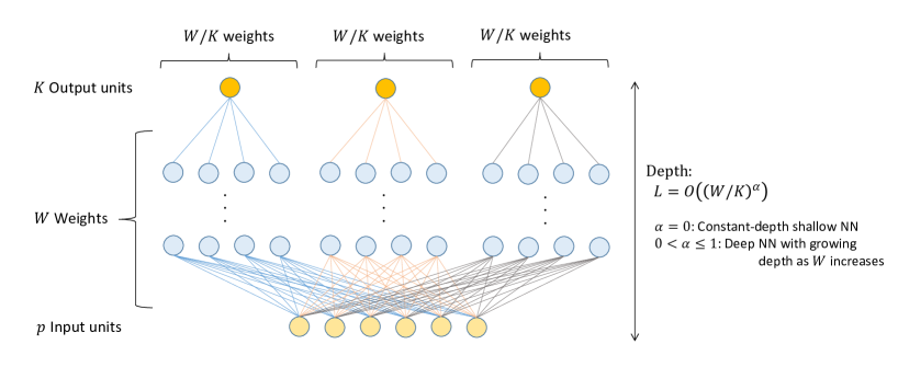
Figure 2: A structure of vector-valued neural network $\boldsymbol{v}_{\text{NN}}:\mathbb{R}^{p}\to\mathbb{R}^{K}$ having $W$ weights. We allocate $W/K$ weights to each output unit, so that weights are not shared by the $K$ output units. In practice, internal units are often shared by the output units, but we consider the above structure for showing the upper bound of the approximation error.

We consider $K$ real-valued neural networks of depth $L=O((W/K)^{\alpha})$ with $W/K$ weights as shown in Fig. 2. Since such NNs are included in $\mathfrak{S}_{\alpha}(W,K)$, we have

$$\inf_{\boldsymbol{v}_{\text{NN}}\in\mathfrak{S}_{\alpha}(W,K)}\sup_{\boldsymbol{x}\in\mathcal{X}}\|\boldsymbol{v}_{*}(\boldsymbol{x}))-\boldsymbol{v}_{\text{NN}}(\boldsymbol{x})\|_{2} \leq\Bigl{(}\sum_{k=1}^{K}\inf_{v_{k}\in\mathfrak{S}_{\alpha}(W/K,1)}\sup_{\boldsymbol{x}\in\mathcal{X}}|v_{*k}(\boldsymbol{x})-v_{k}(\boldsymbol{x})|^{2}\Bigr{)}^{1/2},$$

where $\boldsymbol{v}_{*}(\boldsymbol{x})=(v_{*1}(\boldsymbol{x}),v_{*2}(\boldsymbol{x}),\ldots,v_{*K}(\boldsymbol{x})),\boldsymbol{v}_{\text{NN}}(\boldsymbol{x})=(v_{1}(\boldsymbol{x}),v_{2}(\boldsymbol{x}),\ldots,v_{K}(\boldsymbol{x}))$. We apply Lemma D.2 with $W/K$ weights to each $v_{*k}$, where the same bound $b$ is used in (24). Then the error is bounded by $\sqrt{K}\times abc(W/K)^{-\tfrac{1+\alpha}{p}}=O(K^{\tfrac{1}{2}+\tfrac{1+\alpha}{p}}W^{-\tfrac{1+\alpha}{p}})$. $\Box$

D.3 Proof of Theorem 5.1 (Approximation error rate for IPS)

Applying Theorem 3.1 to a PD kernel $g^{\text{(PD)}}_{*}$, there exist eigenvalues $\{\lambda_{k}\}_{k=1}^{\infty}$, $\lambda_{1}\geq\lambda_{2}\geq\cdots$ and eigenfunctions $\{\phi_{k}(\boldsymbol{y})\}_{k=1}^{\infty}$ such that $\sum_{k=1}^{K}\lambda_{k}\phi_{k}(\boldsymbol{y})\phi_{k}(\boldsymbol{y}^{\prime})$ absolutely and uniformly converges to $g^{\text{(PD)}}_{*}(\boldsymbol{y},\boldsymbol{y}^{\prime})$ as $K\to\infty$. Here, we define two vector-valued functions

$$\boldsymbol{\eta}_{K}(\boldsymbol{y}) :=(\lambda_{1}^{1/2}\phi_{1}(\boldsymbol{y}),\lambda_{2}^{1/2}\phi_{2}(\boldsymbol{y}),\ldots,\lambda_{K}^{1/2}\phi_{K}(\boldsymbol{y})),$$

$$\tilde{\boldsymbol{\phi}}_{K}(\boldsymbol{x}) :=\boldsymbol{\eta}_{K}(\boldsymbol{f}_{*}(\boldsymbol{x})),$$

so that $\displaystyle\langle\boldsymbol{\eta}_{K}(\boldsymbol{f}_{*}(\boldsymbol{x})),\boldsymbol{\eta}_{K}(\boldsymbol{f}_{*}(\boldsymbol{x}^{\prime}))\rangle=\langle\tilde{\boldsymbol{\phi}}_{K}(\boldsymbol{x}),\tilde{\boldsymbol{\phi}}_{K}(\boldsymbol{x}^{\prime})\rangle=\sum_{k=1}^{K}\lambda_{k}\phi_{k}(\boldsymbol{f}_{*}(\boldsymbol{x}))\phi_{k}(\boldsymbol{f}_{*}(\boldsymbol{x}^{\prime}))$. Using these functions, for any $\boldsymbol{f}_{\text{NN}}\in\mathfrak{S}_{\alpha}(W_{f},K)$, we have

$$\bigg{|}g^{\text{(PD)}}_{*}(\boldsymbol{f}_{*}(\boldsymbol{x}),\boldsymbol{f}_{*}(\boldsymbol{x}^{\prime}))-\langle\boldsymbol{f}_{\text{NN}}(\boldsymbol{x}),\boldsymbol{f}_{\text{NN}}(\boldsymbol{x}^{\prime})\rangle\bigg{|}$$

$$\hskip 30.00005pt\leq\bigg{|}g_{*}(\boldsymbol{f}_{*}(\boldsymbol{x}),\boldsymbol{f}_{*}(\boldsymbol{x}^{\prime}))-\langle\boldsymbol{\eta}_{K}(\boldsymbol{f}_{*}(\boldsymbol{x})),\boldsymbol{\eta}_{K}(\boldsymbol{f}_{*}(\boldsymbol{x}^{\prime}))\rangle\bigg{|}$$ (25)

$$\hskip 60.00009pt+\bigg{|}\langle\tilde{\boldsymbol{\phi}}_{K}(\boldsymbol{x}),\tilde{\boldsymbol{\phi}}_{K}(\boldsymbol{x}^{\prime})\rangle-\langle\tilde{\boldsymbol{\phi}}_{K}(\boldsymbol{x}),\boldsymbol{f}_{\text{NN}}(\boldsymbol{x}^{\prime})\rangle\bigg{|}+\bigg{|}\langle\tilde{\boldsymbol{\phi}}_{K}(\boldsymbol{x}),\boldsymbol{f}_{\text{NN}}(\boldsymbol{x}^{\prime})\rangle-\langle\boldsymbol{f}_{\text{NN}}(\boldsymbol{x}),\boldsymbol{f}_{\text{NN}}(\boldsymbol{x}^{\prime})\rangle\bigg{|}.$$ (26)

These terms (25) and (26) can be evaluated in the following way.

• Regarding the term (25),

  $$\sup_{\boldsymbol{x},\boldsymbol{x}^{\prime}\in\mathcal{X}}\bigg{|}g^{\text{(PD)}}_{*}(\boldsymbol{f}_{*}(\boldsymbol{x}),\boldsymbol{f}_{*}(\boldsymbol{x}^{\prime}))-\langle\boldsymbol{\eta}_{K}(\boldsymbol{f}_{*}(\boldsymbol{x})),\boldsymbol{\eta}_{K}(\boldsymbol{f}_{*}(\boldsymbol{x}^{\prime}))\rangle\bigg{|}$$

  $$\hskip 20.00003pt\leq\sup_{\boldsymbol{y},\boldsymbol{y}^{\prime}\in\mathcal{Y}}\bigg{|}g^{\text{(PD)}}_{*}(\boldsymbol{y},\boldsymbol{y}^{\prime})-\langle\boldsymbol{\eta}_{K}(\boldsymbol{y}),\boldsymbol{\eta}_{K}(\boldsymbol{y}^{\prime})\rangle\bigg{|}$$

  $$\hskip 20.00003pt=\sup_{\boldsymbol{y},\boldsymbol{y}^{\prime}\in\mathcal{Y}}\bigg{|}g^{\text{(PD)}}_{*}(\boldsymbol{y},\boldsymbol{y}^{\prime})-\sum_{k=1}^{K}\lambda_{k}\phi_{k}(\boldsymbol{y})\phi_{k}(\boldsymbol{y}^{\prime})\bigg{|}=O(K^{-1/K^{*}}),$$

  where the last formula follows by applying Lemma D.1 to $g^{\text{(PD)}}_{*}$. Thus, we have

  $$\inf_{\boldsymbol{f}_{\text{NN}}\in\mathfrak{S}_{\alpha}(W_{f},K)}\sup_{\boldsymbol{x},\boldsymbol{x}^{\prime}\in\mathcal{X}}\bigg{|}g^{\text{(PD)}}_{*}(\boldsymbol{f}_{*}(\boldsymbol{x}),\boldsymbol{f}_{*}(\boldsymbol{x}^{\prime}))-\langle\boldsymbol{\eta}_{K}(\boldsymbol{f}_{*}(\boldsymbol{x})),\boldsymbol{\eta}_{K}(\boldsymbol{f}_{*}(\boldsymbol{x}^{\prime}))\rangle\bigg{|}=O(K^{-1/K^{*}}).$$ (27)

• Regarding the term (26),

  $$\sup_{\boldsymbol{x},\boldsymbol{x}^{\prime}\in\mathcal{X}}\biggl{\{}\bigg{|}\langle\tilde{\boldsymbol{\phi}}_{K}(\boldsymbol{x}),\tilde{\boldsymbol{\phi}}_{K}(\boldsymbol{x}^{\prime})\rangle-\langle\tilde{\boldsymbol{\phi}}_{K}(\boldsymbol{x}),\boldsymbol{f}_{\text{NN}}(\boldsymbol{x}^{\prime})\rangle\bigg{|}+\bigg{|}\langle\tilde{\boldsymbol{\phi}}_{K}(\boldsymbol{x}),\boldsymbol{f}_{\text{NN}}(\boldsymbol{x}^{\prime})\rangle-\langle\boldsymbol{f}_{\text{NN}}(\boldsymbol{x}),\boldsymbol{f}_{\text{NN}}(\boldsymbol{x}^{\prime})\rangle\bigg{|}\biggr{\}}$$

  $$\leq\sup_{\boldsymbol{x},\boldsymbol{x}^{\prime}\in\mathcal{X}}\biggl{\{}\|\tilde{\boldsymbol{\phi}}_{K}(\boldsymbol{x})\|_{2}\|\tilde{\boldsymbol{\phi}}_{K}(\boldsymbol{x}^{\prime})-\boldsymbol{f}_{\text{NN}}(\boldsymbol{x}^{\prime})\|_{2}+\|\boldsymbol{f}_{\text{NN}}(\boldsymbol{x}^{\prime})\|_{2}\|\tilde{\boldsymbol{\phi}}_{K}(\boldsymbol{x})-\boldsymbol{f}_{\text{NN}}(\boldsymbol{x})\|_{2}\biggr{\}}$$

  $$\leq\sup_{\boldsymbol{x},\boldsymbol{x}^{\prime}\in\mathcal{X}}\biggl{\{}\|\tilde{\boldsymbol{\phi}}_{K}(\boldsymbol{x})\|_{2}\|\tilde{\boldsymbol{\phi}}_{K}(\boldsymbol{x}^{\prime})-\boldsymbol{f}_{\text{NN}}(\boldsymbol{x}^{\prime})\|_{2}+(\|\tilde{\boldsymbol{\phi}}_{K}(\boldsymbol{x}^{\prime})\|_{2}+\|\tilde{\boldsymbol{\phi}}_{K}(\boldsymbol{x}^{\prime})-\boldsymbol{f}_{\text{NN}}(\boldsymbol{x}^{\prime})\|_{2})\|\tilde{\boldsymbol{\phi}}_{K}(\boldsymbol{x})-\boldsymbol{f}_{\text{NN}}(\boldsymbol{x})\|_{2}\biggr{\}}$$

  $$=2\sup_{\boldsymbol{x}\in\mathcal{X}}\|\tilde{\boldsymbol{\phi}}_{K}(\boldsymbol{x})\|_{2}\sup_{\boldsymbol{x}^{\prime}\in\mathcal{X}}\|\tilde{\boldsymbol{\phi}}_{K}(\boldsymbol{x}^{\prime})-\boldsymbol{f}_{\text{NN}}(\boldsymbol{x}^{\prime})\|_{2}+\sup_{\boldsymbol{x}\in\mathcal{X}}\|\tilde{\boldsymbol{\phi}}_{K}(\boldsymbol{x})-\boldsymbol{f}_{\text{NN}}(\boldsymbol{x})\|_{2}^{2}.$$

  Here, $\|\tilde{\boldsymbol{\phi}}_{K}(\boldsymbol{x})\|_{2}=\|\sum_{k=1}^{K}\lambda_{k}\phi_{k}(\boldsymbol{f}_{*}(\boldsymbol{x}))\phi_{k}(\boldsymbol{f}_{*}(\boldsymbol{x}))\|_{2}\leq\|\sum_{k=1}^{\infty}\lambda_{k}\phi_{k}(\boldsymbol{f}_{*}(\boldsymbol{x}))\phi_{k}(\boldsymbol{f}_{*}(\boldsymbol{x}))\|_{2}=\|g^{\text{(PD)}}_{*}(\boldsymbol{f}_{*}(\boldsymbol{x}),\boldsymbol{f}_{*}(\boldsymbol{x}))\|_{2}$ is bounded, because $g^{\text{(PD)}}_{*}(\boldsymbol{f}_{*}(\boldsymbol{x}),\boldsymbol{f}_{*}(\boldsymbol{x}))$ is continuous over the compact set $\mathcal{X}^{2}$. For applying Lemma D.3 to $\tilde{\boldsymbol{\phi}}_{K}(\boldsymbol{x})$, we need to show that the constant $b$ exists. Noting $\|\partial\tilde{\phi}_{k}/\partial\boldsymbol{x}\|_{2}^{2}=\sum_{i=1}^{p}(\partial\tilde{\phi}_{k}/\partial x_{i})^{2}\leq\sum_{i=1}^{p}\lambda_{k}\|\partial\phi_{k}/\partial\boldsymbol{y}\|_{2}^{2}\,\|\partial\boldsymbol{f}_{*}/\partial x_{i}\|_{2}^{2}$, we have

  $$\sup_{k\in\mathbb{N}}\sup_{\boldsymbol{x}\in\mathcal{X}}\|\partial\tilde{\phi}_{k}/\partial\boldsymbol{x}\|_{2}^{2}\leq\sup_{k\in\mathbb{N}}\sup_{\boldsymbol{y}\in\mathcal{Y}}\lambda_{k}\|\partial\phi_{k}/\partial\boldsymbol{y}\|_{2}^{2}\,\sup_{\boldsymbol{x}\in\mathcal{X}}\sum_{i=1}^{p}\|\partial\boldsymbol{f}_{*}/\partial x_{i}\|_{2}^{2}<\infty,$$ (28)

  where $\sup_{k\in\mathbb{N}}\sup_{\boldsymbol{y}\in\mathcal{Y}}\lambda_{k}\|\partial\phi_{k}/\partial\boldsymbol{y}\|_{2}^{2}<\infty$ follows from (C-1) and $\sup_{\boldsymbol{x}\in\mathcal{X}}\sum_{i=1}^{p}\|\partial\boldsymbol{f}_{*}/\partial x_{i}\|_{2}^{2}<\infty$ follows from (C-3). We can take $b^{2}$ as the upper bound of (28), and then Lemma D.3 implies

  $$\inf_{\boldsymbol{f}_{\text{NN}}\in\mathfrak{S}_{\alpha}(W_{f},K)}\sup_{\boldsymbol{x}\in\mathcal{X}}\|\tilde{\boldsymbol{\phi}}_{K}(\boldsymbol{x})-\boldsymbol{f}_{\text{NN}}(\boldsymbol{x})\|_{2}=O(K^{\tfrac{1}{2}+\tfrac{1+\alpha}{p}}W_{f}^{-\tfrac{1+\alpha}{p}})$$ (29)

  so that the evaluation of (26) leads to

  $$\hskip 30.00005pt=O(K^{\tfrac{1}{2}+\tfrac{1+\alpha}{p}}W_{f}^{-\tfrac{1+\alpha}{p}}).$$ (30)

Considering (27) and (30), we finally obtain

$$\inf_{\boldsymbol{f}_{\text{NN}}\in\mathfrak{S}_{\sigma}(W_{f},K)}\sup_{\boldsymbol{x},\boldsymbol{x}^{\prime}\in\mathcal{X}}\bigg{|}g^{\text{(PD)}}_{*}(\boldsymbol{f}_{*}(\boldsymbol{x}),\boldsymbol{f}_{*}(\boldsymbol{x}^{\prime}))-\langle\boldsymbol{f}_{\text{NN}}(\boldsymbol{x}),\boldsymbol{f}_{\text{NN}}(\boldsymbol{x}^{\prime})\rangle\bigg{|}=O\Bigl{(}K^{-\tfrac{1}{K^{*}}}+K^{\tfrac{1}{2}+\tfrac{1+\alpha}{p}}W_{f}^{-\tfrac{1+\alpha}{p}}\Bigr{)}.$$

$\Box$

D.4 Proof of Theorem 5.2 (Approximation error rate for SIPS)

Recall the inequality (17) in Section C.2.

$$\sup_{\boldsymbol{x},\boldsymbol{x}^{\prime}\in\mathcal{X}}\bigg{|}g^{\text{(CPD)}}_{*}(\boldsymbol{f}_{*}(\boldsymbol{x}),\boldsymbol{f}_{*}(\boldsymbol{x}^{\prime}))-(\langle\boldsymbol{f}_{\text{NN}}(\boldsymbol{x}),\boldsymbol{f}_{\text{NN}}(\boldsymbol{x}^{\prime})\rangle+u_{\text{NN}}(\boldsymbol{x})+u_{\text{NN}}(\boldsymbol{x}^{\prime}))\bigg{|}$$

$$\hskip 20.00003pt\leq\sup_{\boldsymbol{x},\boldsymbol{x}^{\prime}\in\mathcal{X}}\bigg{|}g_{0}(\boldsymbol{f}_{*}(\boldsymbol{x}),\boldsymbol{f}_{*}(\boldsymbol{x}^{\prime}))-\langle\boldsymbol{f}_{\text{NN}}(\boldsymbol{x}),\boldsymbol{f}_{\text{NN}}(\boldsymbol{x}^{\prime})\rangle\bigg{|}+2\sup_{\boldsymbol{x}\in\mathcal{X}}\bigg{|}h_{*}(\boldsymbol{x})-u_{\text{NN}}(\boldsymbol{x})\bigg{|}$$ (31)

We evaluate the two terms in (31). Since we have assumed that $g^{\text{(CPD)}}_{*}$ is $C^{1}$ (the condition C-2), $g_{0}$ and $h_{*}$ are also $C^{1}$. Then, by applying Theorem 5.1 to the PD kernel $g_{0}$, the first term in (31) is evaluated as

$$\inf_{\boldsymbol{f}_{\text{NN}}\in\mathfrak{S}_{\alpha}(W_{f},K)}\sup_{\boldsymbol{x},\boldsymbol{x}^{\prime}\in\mathcal{X}}\bigg{|}g_{0}(\boldsymbol{f}_{*}(\boldsymbol{x}),\boldsymbol{f}_{*}(\boldsymbol{x}^{\prime}))-\langle\boldsymbol{f}_{\text{NN}}(\boldsymbol{x}),\boldsymbol{f}_{\text{NN}}(\boldsymbol{x}^{\prime})\rangle\bigg{|}=O\Bigl{(}K^{-\tfrac{1}{K^{*}}}+K^{\tfrac{1}{2}+\tfrac{1+\alpha}{p}}W_{f}^{-\tfrac{1+\alpha}{p}}\Bigr{)}.$$ (32)

By applying Lemma D.2 to $h_{*}$, the second term in (31) is evaluated as

$$\inf_{u_{\text{NN}}\in\mathfrak{S}_{\alpha}(W_{u},1)}\sup_{\boldsymbol{x}\in\mathcal{X}}\bigg{|}h_{*}(\boldsymbol{x})-u_{\text{NN}}(\boldsymbol{x})\bigg{|}=O\Bigl{(}W_{u}^{-\tfrac{1+\alpha}{p}}\Bigr{)}.$$ (33)

Considering (31), (32) and (33), we obtain

$$\inf_{\begin{subarray}{c}\boldsymbol{f}_{\text{NN}}\in\mathfrak{S}_{\alpha}(W_{f},K)\\ u_{\text{NN}}\in\mathfrak{S}_{\alpha}(W_{u},1)\end{subarray}}\sup_{\boldsymbol{x},\boldsymbol{x}^{\prime}\in\mathcal{X}}\bigg{|}g^{\text{(CPD)}}_{*}(\boldsymbol{f}_{*}(\boldsymbol{x}),\boldsymbol{f}_{*}(\boldsymbol{x}^{\prime}))-(\langle\boldsymbol{f}_{\text{NN}}(\boldsymbol{x}),\boldsymbol{f}_{\text{NN}}(\boldsymbol{x}^{\prime})\rangle+u_{\text{NN}}(\boldsymbol{x})+u_{\text{NN}}(\boldsymbol{x}^{\prime}))\bigg{|}$$

$$\hskip 30.00005pt=O\Bigl{(}K^{-\tfrac{1}{K^{*}}}+K^{\tfrac{1}{2}+\tfrac{1+\alpha}{p}}W_{f}^{-\tfrac{1+\alpha}{p}}+W_{u}^{-\tfrac{1+\alpha}{p}}\Bigr{)}.$$

$\Box$

Appendix E Non-CPD Similarities

CPD includes a broad range of kernels, but there exists a variety of non-CPD kernels. One example is Epanechnikov kernel $g(\boldsymbol{y},\boldsymbol{y}^{\prime}):=(1-\|\boldsymbol{y}-\boldsymbol{y}^{\prime}\|_{2}^{2})\boldsymbol{1}(\|\boldsymbol{y}-\boldsymbol{y}^{\prime}\|_{2}\leq 1)$. To approximate similarities based on such non-CPD kernels, we propose a novel model, yet based on inner product, with high approximation capability beyond SIPS. Although parameter optimization of this model is not always easy due to the excessive degrees of freedom, the model is, in theory, shown to be capable of approximating more general kernels that are considered in Ong et al., (2004).

E.1 Proposed model

Let us consider a similarity $h(\boldsymbol{x},\boldsymbol{x}^{\prime})=g_{*}(f_{*}(\boldsymbol{x}),f_{*}(\boldsymbol{x}^{\prime}))$ with any kernel $g_{*}:\mathbb{R}^{2K^{*}}\to\mathbb{R}$ and a continuous map $f_{*}:\mathbb{R}^{p}\to\mathbb{R}^{K^{*}}$. To approximate it, we consider a similarity model

$$h(\boldsymbol{x}_{i},\boldsymbol{x}_{j})=\langle\boldsymbol{f}_{\text{NN}}(\boldsymbol{x}_{i}),\boldsymbol{f}_{\text{NN}}(\boldsymbol{x}_{j})\rangle-\langle\boldsymbol{r}_{\text{NN}}(\boldsymbol{x}_{i}),\boldsymbol{r}_{\text{NN}}(\boldsymbol{x}_{j})\rangle,$$ (34)

where $\boldsymbol{f}_{\text{NN}}:\mathbb{R}^{p}\to\mathbb{R}^{K_{+}}$ and $\boldsymbol{r}_{\text{NN}}:\mathbb{R}^{p}\to\mathbb{R}^{K_{-}}$ are neural networks. Since the kernel $g(\boldsymbol{y},\boldsymbol{y}^{\prime})=\langle\boldsymbol{y}_{+},\boldsymbol{y}^{\prime}_{+}\rangle-\langle\boldsymbol{y}_{-},\boldsymbol{y}^{\prime}_{-}\rangle$ with respect to $\boldsymbol{y}=(\boldsymbol{y}_{+},\boldsymbol{y}_{-})\in\mathbb{R}^{K_{+}+K_{-}}$ represents the difference of two IPSs, we call (34) as inner product difference similarity (IPDS) model.

By replacing $\boldsymbol{f}_{\text{NN}}(\boldsymbol{x})$ and $\boldsymbol{r}_{\text{NN}}(\boldsymbol{x})$ with $(\boldsymbol{f}_{\text{NN}}(\boldsymbol{x})^{\top},u_{\text{NN}}(\boldsymbol{x}),1)^{\top}$ and $u_{\text{NN}}(\boldsymbol{x})-1\in\mathbb{R}$, respectively, IPDS reduces to SIPS defined in eq. (6), meaning that IPDS includes SIPS as a special case. Therefore, IPDS approximates any CPD similarities arbitrary well. Further, we prove that IPDS approximates more general similarities arbitrary well.

E.2 Approximation theorem

Theorem E.1 (Approximation theorem for IPDS)

Symbols and assumptions are the same as those of Theorem 4.1 but $g_{*}$ is a general kernel, which is only required to be dominated by some PD kernels $g$, i.e., $g-g_{*}$ is PD. For arbitrary $\varepsilon>0$, by specifying sufficiently large $K_{+},K_{-}\in\mathbb{N},m_{+}=m_{+}(K_{+}),m_{-}=m_{-}(K_{-})\in\mathbb{N}$, there exist $\boldsymbol{A}\in\mathbb{R}^{K_{+}\times m_{+}},\boldsymbol{B}\in\mathbb{R}^{m_{+}\times p},\boldsymbol{c}\in\mathbb{R}^{m_{+}},\boldsymbol{E}\in\mathbb{R}^{K_{-}\times m_{-}},\boldsymbol{F}\in\mathbb{R}^{m_{-}\times p},\boldsymbol{o}\in\mathbb{R}^{m_{-}}$ such that

for all $(\boldsymbol{x},\boldsymbol{x}^{\prime})\in[-M,M]^{2p}$, where $\boldsymbol{f}_{\text{NN}}(\boldsymbol{x})=\boldsymbol{A}\boldsymbol{\sigma}(\boldsymbol{B}\boldsymbol{x}+\boldsymbol{c})\in\mathbb{R}^{K_{+}}$ and $\boldsymbol{r}_{\text{NN}}(x)=\boldsymbol{E}\boldsymbol{\sigma}(\boldsymbol{F}\boldsymbol{x}+\boldsymbol{o})\in\mathbb{R}^{K_{-}}$ are 1-hidden layer neural networks with $m_{+}$ and $m_{-}$ hidden units, respectively.

In theorem E.1, the kernel $g_{*}$ is only required to be dominated by some PD kernels, thus $g_{*}$ is not limited to CPD. We call such a kernel $g_{*}$ satisfying the condition in Theorem E.1, i.e., there exists a PD kernel $g$ such that $g-g_{*}$ is PD, as general kernel, and the general kernel $g_{*}$ is called indefinite if neither of $g_{*},-g_{*}$ is positive definite (Ong et al.,, 2004). General similarity and indefinite similarity are defined as well; IPDS approximates any general similarities arbitrary well.

Our proof for Theorem E.1 is based on Proposition 7 of Ong et al., (2004). This proposition indicates that the kernel $g_{*}$ dominated by some PD kernels is decomposed as the difference of two PD kernels $g_{+},g_{-}$ by considering Krein space consisting of two Hilbert spaces. Therefore, we have $g_{*}(\boldsymbol{f}_{*}(\boldsymbol{x}),\boldsymbol{f}_{*}(\boldsymbol{x}^{\prime}))=g_{+}(\boldsymbol{f}_{*}(\boldsymbol{x}),\boldsymbol{f}_{*}(\boldsymbol{x}^{\prime}))-g_{-}(\boldsymbol{f}_{*}(\boldsymbol{x}),\boldsymbol{f}_{*}(\boldsymbol{x}^{\prime}))$. Because of the PD-ness of $g_{+}$ and $g_{-}$, Theorem 3.2 guarantees the existence of NNs $\boldsymbol{f}_{\text{NN}},\boldsymbol{r}_{\text{NN}}$ such that $\langle\boldsymbol{f}_{\text{NN}}(\boldsymbol{x}),\boldsymbol{f}_{\text{NN}}(\boldsymbol{x}^{\prime})\rangle$ and $\langle\boldsymbol{r}_{\text{NN}}(\boldsymbol{x}),\boldsymbol{r}_{\text{NN}}(\boldsymbol{x}^{\prime})\rangle$, respectively, approximate $g_{+}(\boldsymbol{f}_{*}(\boldsymbol{x}),\boldsymbol{f}_{*}(\boldsymbol{x}^{\prime}))$ and $g_{-}(\boldsymbol{f}_{*}(\boldsymbol{x}),\boldsymbol{f}_{*}(\boldsymbol{x}^{\prime}))$ arbitrary well. Thus proving the theorem. This idea for the proof is also interpreted as a generalized Mercer’s theorem for Krein space (there is a similar attempt in Chen et al., (2008)) by applying Mercer’s theorem to the two Hilbert spaces of Ong et al., (2004, Proposition 7).

E.3 Deep Gaussian embedding

To show another example of non-CPD kernels, Deep Gaussian embedding (Bojchevski and Günnemann,, 2018) is reviewed below.

Example E.1 (Deep Gaussian embedding)

Let $\mathcal{Y}$ be a set of distributions over a set $\boldsymbol{Z}\subset\mathbb{R}^{q}$. Kullback-Leibler divergence (Kullback and Leibler,, 1951) between two distributions $\boldsymbol{y},\boldsymbol{y}^{\prime}\in\mathcal{Y}$ is defined by

$$d_{\text{KL}}(\boldsymbol{y},\boldsymbol{y}^{\prime}):=\int_{\boldsymbol{Z}}y(\boldsymbol{z})\log\frac{y(\boldsymbol{z})}{y^{\prime}(\boldsymbol{z})}\mathrm{d}\boldsymbol{z},$$

where $y(\boldsymbol{z})$ is the probability density function corresponding to the distribution $\boldsymbol{y}\in\mathcal{Y}$.

With the same setting in Section 2, Deep Gaussian embedding (Bojchevski and Günnemann,, 2018), which incorporates neural networks into Gaussian embedding (Vilnis and McCallum,, 2015), learns two neural networks $\boldsymbol{\mu}:\mathbb{R}^{p}\to\mathbb{R}^{q},\boldsymbol{\Sigma}:\mathbb{R}^{p}\to\mathbb{R}^{q\times q}_{+}$ so that the function $\sigma(-d_{\text{KL}}(\mathcal{N}_{q}(\boldsymbol{\mu}(\boldsymbol{x}_{i}),\boldsymbol{\Sigma}(\boldsymbol{x}_{i})),\mathcal{N}_{q}(\boldsymbol{\mu}(\boldsymbol{x}_{j}),\boldsymbol{\Sigma}(\boldsymbol{x}_{j}))))$ approximates $E(w_{ij}|\boldsymbol{x}_{i},\boldsymbol{x}_{j})$. $\mathbb{R}_{+}^{q\times q}$ is a set of all $q\times q$ positive definite matrices and $\mathcal{N}_{q}(\boldsymbol{\mu},\boldsymbol{\Sigma})$ represents the $q$-variate normal distribution with mean $\boldsymbol{\mu}$ and variance-covariance matrix $\boldsymbol{\Sigma}$.

Unlike typical graph embedding methods, deep Gaussian embedding maps data vectors to distributions as

$$\mathbb{R}^{p}\ni\boldsymbol{x}\mapsto\boldsymbol{y}:=\mathcal{N}_{q}(\boldsymbol{\mu}(\boldsymbol{x}),\boldsymbol{\Sigma}(\boldsymbol{x}))\in\mathcal{Y},$$

where $\boldsymbol{y}$ is also interpreted as a vector of dimension $K=q+q(q+1)/2$ by considering the number of parameters in $\boldsymbol{\mu}$ and $\boldsymbol{\Sigma}$. Our concern is to clarify if $d_{\text{KL}}$ is CPD. However, in the first place, $d_{\text{KL}}$ is not a kernel since it is not symmetric. In order to make it symmetric, Kullback-Leibler divergence may be replaced with Jeffrey’s divergence (Kullback and Leibler,, 1951)

$$d_{\text{Jeff}}(\boldsymbol{y},\boldsymbol{y}^{\prime}):=d_{\text{KL}}(\boldsymbol{y},\boldsymbol{y}^{\prime})+d_{\text{KL}}(\boldsymbol{y}^{\prime},\boldsymbol{y}).$$

Although $-d_{\text{Jeff}}$ is a kernel, it is not CPD as shown in Proposition E.1.

Proposition E.1

$-d_{\text{Jeff}}$ is not CPD on $\tilde{\mathcal{P}}_{q}^{2}$, where $\tilde{\mathcal{P}}_{q}$ represents the set of all $q$-variate normal distributions.

A counterexample of CPD-ness is, $n=3,q=2,c_{1}=-2/5,c_{2}=-3/5,c_{3}=1,\boldsymbol{y}_{i}=\mathcal{N}_{2}(\boldsymbol{\mu}_{i},\boldsymbol{\Sigma}_{i})\in\mathcal{Y}\>(i=1,2,3),\boldsymbol{\mu}_{1}=(2,1)^{\top},\boldsymbol{\mu}_{2}=(-1,1)^{\top},\boldsymbol{\mu}_{3}=(1,2)^{\top},\boldsymbol{\Sigma}_{1}=\mathrm{diag}(1/10,1),\boldsymbol{\Sigma}_{2}=\mathrm{diag}(1/2,1),\boldsymbol{\Sigma}_{3}=\mathrm{diag}(1,1)$.

We are yet studying the nature of deep Gaussian embedding. However, as Proposition E.1 shows, negative Jeffrey’s divergence used in the embedding is already proved to be non-CPD; SIPS cannot approximate it. IPDS model is required for approximating such non-CPD kernels. Thus we are currently trying to reveal to what extent IPDS applies, by classifying whether each of non-CPD kernels including negative Jeffrey’s divergence satisfies the assumption on the kernel $g_{*}$ in Theorem E.1.

References

- Andrew et al., (2013) Andrew, G., Arora, R., Bilmes, J., and Livescu, K. (2013). Deep Canonical Correlation Analysis. In Proceedings of the International Conference on Machine Learning (ICML), pages 1247–1255.
- Arjovsky et al., (2017) Arjovsky, M., Chintala, S., and Bottou, L. (2017). Wasserstein GAN. arXiv preprint arXiv:1701.07875.
- Berg et al., (1984) Berg, C., Christensen, J., and Ressel, P. (1984). Harmonic Analysis on Semigroups: Theory of Positive Definite and Related Functions. Graduate Texts in Mathematics. Springer New York.
- Bradley, (1997) Bradley, A. P. (1997). The Use of the Area Under the ROC Curve in the Evaluation of Machine Learning Algorithms. Pattern Recognition, 30(7):1145–1159.
- Bromley et al., (1994) Bromley, J., Guyon, I., LeCun, Y., Säckinger, E., and Shah, R. (1994). Signature verification using a” siamese” time delay neural network. In Advances in neural information processing systems, pages 737–744.
- Cai et al., (2018) Cai, H., Zheng, V. W., and Chang, K. (2018). A comprehensive survey of graph embedding: problems, techniques and applications. IEEE Transactions on Knowledge and Data Engineering.
- Cobos and Kühn, (1990) Cobos, F. and Kühn, T. (1990). Eigenvalues of integral operators with positive definite kernels satisfying integrated hölder conditions over metric compacta. Journal of Approximation Theory, 63(1):39–55.
- Cybenko, (1989) Cybenko, G. (1989). Approximation by Superpositions of a Sigmoidal Function. Mathematics of Control, Signals, and Systems (MCSS), 2(4):303–314.
- Dai et al., (2018) Dai, Q., Li, Q., Tang, J., and Wang, D. (2018). Adversarial Network Embedding. In Proceedings of the AAAI Conference on Artificial Intelligence (AAAI).
- Faraut and Harzallah, (1974) Faraut, J. and Harzallah, K. (1974). Distances hilbertiennes invariantes sur un espace homogène. In Annales de l’institut Fourier, volume 24, pages 171–217. Association des Annales de l’Institut Fourier.
- Funahashi, (1989) Funahashi, K.-I. (1989). On the approximate realization of continuous mappings by neural networks. Neural Networks, 2(3):183–192.
- Gardner et al., (2017) Gardner, A., Duncan, C. A., Kanno, J., and Selmic, R. R. (2017). On the Definiteness of Earth Mover’s Distance and Its Relation to Set Intersection. IEEE Transactions on Cybernetics.
- Grover and Leskovec, (2016) Grover, A. and Leskovec, J. (2016). node2vec: Scalable Feature Learning for Networks. In Proceedings of the ACM International Conference on Knowledge Discovery and Data mining (SIGKDD), pages 855–864. ACM.
- Hamilton et al., (2017) Hamilton, W. L., Ying, Z., and Leskovec, J. (2017). Inductive Representation Learning on Large Graphs. Advances in Neural Information Processing Systems (NIPS), pages 1025–1035.
- He et al., (2015) He, K., Zhang, X., Ren, S., and Sun, J. (2015). Delving Deep into Rectifiers: Surpassing Human-Level Performance on ImageNet Classification. arXiv preprint arXiv:1502.01852.
- He and Niyogi, (2004) He, X. and Niyogi, P. (2004). Locality Preserving Projections. In Advances in Neural Information Processing Systems (NIPS), pages 153–160.
- Hofmann et al., (2008) Hofmann, T., Schölkopf, B., and Smola, A. J. (2008). Kernel methods in machine learning. The annals of statistics, pages 1171–1220.
- Huang et al., (2012) Huang, Z., Shan, S., Zhang, H., Lao, S., and Chen, X. (2012). Cross-view Graph Embedding. In Proceedings of the Asian Conference on Computer Vision (ACCV), pages 770–781.
- Kingma and Ba, (2014) Kingma, D. P. and Ba, J. (2014). Adam: A Method for Stochastic Optimization. arXiv preprint arXiv:1412.6980.
- Kipf and Welling, (2016) Kipf, T. N. and Welling, M. (2016). Variational Graph Auto-Encoders. NIPS Workshop.
- Kolouri et al., (2016) Kolouri, S., Zou, Y., and Rohde, G. K. (2016). Sliced Wasserstein kernels for probability distributions. In Proceedings of the IEEE Conference on Computer Vision and Pattern Recognition (CVPR), pages 5258–5267.
- Koren et al., (2009) Koren, Y., Bell, R., and Volinsky, C. (2009). Matrix factorization techniques for recommender systems. Computer, (8):30–37.
- Levy and Goldberg, (2014) Levy, O. and Goldberg, Y. (2014). Linguistic regularities in sparse and explicit word representations. In Proceedings of the eighteenth conference on computational natural language learning, pages 171–180.
- (24) Mikolov, T., Sutskever, I., Chen, K., Corrado, G. S., and Dean, J. (2013a). Distributed Representations of Words and Phrases and their Compositionality. In Advances in Neural Information Processing Systems (NIPS), pages 3111–3119.
- (25) Mikolov, T., Yih, W.-t., and Zweig, G. (2013b). Linguistic regularities in continuous space word representations. In Proceedings of the 2013 Conference of the North American Chapter of the Association for Computational Linguistics: Human Language Technologies, pages 746–751.
- Miller, (1995) Miller, G. A. (1995). WordNet: a lexical database for English. Communications of the ACM, 38(11):39–41.
- Minh et al., (2006) Minh, H. Q., Niyogi, P., and Yao, Y. (2006). Mercer’s Theorem, Feature Maps, and Smoothing. In International Conference on Computational Learning Theory (COLT), pages 154–168. Springer.
- Nickel and Kiela, (2017) Nickel, M. and Kiela, D. (2017). Poincaré embeddings for learning hierarchical representations. In Advances in Neural Information Processing Systems (NIPS), pages 6341–6350.
- Nickel and Kiela, (2018) Nickel, M. and Kiela, D. (2018). Learning continuous hierarchies in the lorentz model of hyperbolic geometry. In Proceedings of the International Conference on Machine Learning (ICML).
- Okuno et al., (2018) Okuno, A., Hada, T., and Shimodaira, H. (2018). A probabilistic framework for multi-view feature learning with many-to-many associations via neural networks. In Proceedings of the International Conference on Machine Learning (ICML), pages 3885–3894.
- Okuno and Shimodaira, (2018) Okuno, A. and Shimodaira, H. (2018). On representation power of neural network-based graph embedding and beyond. In ICML Workshop (TADGM).
- Pennington et al., (2014) Pennington, J., Socher, R., and Manning, C. (2014). GloVe: Global Vectors for Word Representation. In Proceedings of the Conference on Empirical Methods in Natural Language Processing (EMNLP), pages 1532–1543.
- Perozzi et al., (2014) Perozzi, B., Al-Rfou, R., and Skiena, S. (2014). DeepWalk: Online Learning of Social Representations. In Proceedings of the ACM International Conference on Knowledge Discovery and Data mining (SIGKDD), pages 701–710. ACM.
- Prado et al., (2013) Prado, A., Plantevit, M., Robardet, C., and Boulicaut, J.-F. (2013). Mining graph topological patterns: Finding covariations among vertex descriptors. IEEE Transactions on Knowledge and Data Engineering, 25(9):2090–2104.
- Sarkar, (2011) Sarkar, R. (2011). Low Distortion Delaunay Embedding of Trees in Hyperbolic Plane. In International Symposium on Graph Drawing, pages 355–366. Springer.
- Schölkopf, (2001) Schölkopf, B. (2001). The kernel trick for distances. In Advances in Neural Information Processing Systems (NIPS), pages 301–307.
- Shimodaira, (2016) Shimodaira, H. (2016). Cross-validation of matching correlation analysis by resampling matching weights. Neural Networks, 75:126–140.
- Tang et al., (2015) Tang, J., Qu, M., Wang, M., Zhang, M., Yan, J., and Mei, Q. (2015). LINE: Large-scale Information Network Embedding. In Proceedings of the International Conference on World Wide Web (WWW), pages 1067–1077.
- Telgarsky, (2017) Telgarsky, M. (2017). Neural networks and rational functions. In Proceedings of the International Conference on Machine Learning (ICML).
- Tolstikhin et al., (2018) Tolstikhin, I., Bousquet, O., Gelly, S., and Schoelkopf, B. (2018). Wasserstein Auto-Encoders. In Proceedings of the International Conference on Representation Learning (ICLR).
- Yan et al., (2007) Yan, S., Xu, D., Zhang, B., Zhang, H.-J., Yang, Q., and Lin, S. (2007). Graph Embedding and Extensions: A General Framework for Dimensionality Reduction. IEEE transactions on Pattern Analysis and Machine Intelligence (PAMI), 29(1):40–51.
- Yarotsky, (2017) Yarotsky, D. (2017). Error bounds for approximations with deep ReLU networks. Neural Networks, 94:103–114.
- Yarotsky, (2018) Yarotsky, D. (2018). Optimal approximation of continuous functions by very deep ReLU networks. Proceedings of Machine Learning Research, 75:639–649. The 31st Annual Conference on Learning Theory (COLT 2018).
- Zhanga et al., (2017) Zhanga, D., Yinb, J., Zhuc, X., and Zhanga, C. (2017). User profile preserving social network embedding. In Proceedings of the AAAI Conference on Artificial Intelligence (AAAI).
Supplementary Material:
Graph Embedding with Shifted Inner Product Similarity and Its Improved Approximation Capability

References

- Berg et al., (1984) Berg, C., Christensen, J., and Ressel, P. (1984). Harmonic Analysis on Semigroups: Theory of Positive Definite and Related Functions. Graduate Texts in Mathematics. Springer New York.
- Bojchevski and Günnemann, (2018) Bojchevski, A. and Günnemann, S. (2018). Deep gaussian embedding of attributed graphs: Unsupervised inductive learning via ranking. In Proceedings of the International Conference on Learning Representations (ICLR).
- Chen et al., (2008) Chen, D.-G., Wang, H.-Y., and Tsang, E. C. (2008). Generalized Mercer theorem and its application to feature space related to indefinite kernels. In Proceedings of the International Conference on Machine Learning and Cybernetics (ICMLC), volume 2, pages 774–777. IEEE.
- Cobos and Kühn, (1990) Cobos, F. and Kühn, T. (1990). Eigenvalues of integral operators with positive definite kernels satisfying integrated hölder conditions over metric compacta. Journal of Approximation Theory, 63(1):39–55.
- Cybenko, (1989) Cybenko, G. (1989). Approximation by Superpositions of a Sigmoidal Function. Mathematics of Control, Signals, and Systems (MCSS), 2(4):303–314.
- Kullback and Leibler, (1951) Kullback, S. and Leibler, R. A. (1951). On information and sufficiency. The annals of mathematical statistics, 22(1):79–86.
- Naber, (2012) Naber, G. L. (2012). The geometry of Minkowski spacetime: An introduction to the mathematics of the special theory of relativity, volume 92. Springer Science & Business Media.
- Nickel and Kiela, (2017) Nickel, M. and Kiela, D. (2017). Poincaré embeddings for learning hierarchical representations. In Advances in Neural Information Processing Systems (NIPS), pages 6341–6350.
- Okuno et al., (2018) Okuno, A., Hada, T., and Shimodaira, H. (2018). A probabilistic framework for multi-view feature learning with many-to-many associations via neural networks. In Proceedings of the International Conference on Machine Learning (ICML), pages 3885–3894.
- Ong et al., (2004) Ong, C. S., Mary, X., Canu, S., and Smola, A. J. (2004). Learning with non-positive kernels. In Proceedings of the International Conference on Machine Learning (ICML), page 81. ACM.
- Telgarsky, (2017) Telgarsky, M. (2017). Neural networks and rational functions. In Proceedings of the International Conference on Machine Learning (ICML).
- Vilnis and McCallum, (2015) Vilnis, L. and McCallum, A. (2015). Word representations via gaussian embedding. In Proceedings of the International Conference on Learning Representations (ICLR).
- Yarotsky, (2018) Yarotsky, D. (2018). Optimal approximation of continuous functions by very deep ReLU networks. Proceedings of Machine Learning Research, 75:639–649. The 31st Annual Conference on Learning Theory (COLT 2018).