Two-impurity-entanglement generation by electron scattering in zigzag phosphorene nanoribbons

Abstract

In this paper, we investigate how two on-side doped impurities with net magnetic moments in an edge chain of a zigzag phosphorene nanoribbon (zPNR) can be entangled by scattering of the traveling edge-state electrons. To this end, in the first step, we employ the Lippmann-Scwinger equation as well as the Green’s function approach to study the scattering of the free traveling electrons from two magnetic impurities in a one-dimensional tight-binding chain. Then, following the same formalism, that is shown that the behavior of two on-side spin impurities in the edge chain of a zPNR in responding to the scattering of the edge-state traveling electrons is very similar to what happens for the one-dimensional chain. In both cases, considering a known incoming wave state, the reflected and transmitted parts of the final wave state are evaluated analytically. Using the obtained results, the related partial density matrices and the reflection and transmission probabilities are computable. Negativity as a measure of the produced entanglement in the final state is calculated and the results are discussed. Our theoretical model actually proposes a method, which is perhaps experimentally performable to create the entanglement in the state of the impurities .

I Introduction 

Since the realization of phosphorene Liu2014 , as an atomic layer of phosphorus, it has attracted great attention due to its physical properties and possible applications Carvalho2016 ; Ling2015 . This new specimen of 2D material is a layered crystal of phosphorus atoms which are covalently bonded with three nearest neighbors via $sp^{3}$ hybridization to form a puckered 2D honeycomb structure. It is this unique property of anisotropy together with a large direct band gap that makes phosphorene a desirable candidate material for different applications with specific electronic, mechanical, thermal, and transport features Neto2014 ; Qiao2014 ; Peeters2014 ; Guinea2014 ; Yang2014 ; Katsnelson2015 ; Asgari2015 . Moreover, phosphorene like the other 2D nanomaterials can be patterned into phosphorene nanoribbons (PNR) which can be fabricated with lithography and plasma etching of black-phosphorus Feng2015 ; Maity2016 ; Fang2017 . The phosphorene ribbon with zigzag edges, which is called zigzag phosphorene nanoribbon (zPNR), shows degenerate quasi-flat bands in the middle of the gap that separates the valence and conduction bands Ezawa2014 . Furthermore, due to the existence of such a gap that protects the quasi-flat band, the quantum transport of these localized edge sates are found to be, in some sense, like a quasi-one dimensional chain both numerically and analytically Ezawa2014 ; Asgari2018 .

On the other hand, one of the interesting aspects of modern quantum mechanics is to share quantum information and create entanglement between the components of a quantum-scale system. One of the ways to this end is to use the scattering phenomena. In a number of pervious studies in this field, adopting a free electron model, the entanglement generation created due to one-dimensional scattering of electrons from Kondo and Heisenberg impurities has been theoretically investigated Ghanbari2013 ; Ghanbari2015 ; Ghanbari2016 . Also, in one of these studies, it was shown that the Klein tunneling effect of the traveling electrons in a graphene sheet can leads to a correlation between the transmitted and the reflected electrons and also between the quantum-dot spin qubits fixed in the graphene nanoribbons Ghanbari2016 . However, the differences between the electronic spectrum of the graphene and phosphorene nanostructures can motivate development of such studies to nanostructures based on phosphorus. In fact, one of the significant aspects of the edge states in zPNR might be the fingerprints of these states on the entanglement generation between two localized magnetic impurities on the edges through the scattering of electrons by such impurities. In the present work, scattering of the ballistic electrons by the quantum-dot spin qubits fixed at the edges of a zPNR is investigated theoretically. To this end, since the phospherene edge states in a zigzag nanoribbon exhibit like a one-dimensional tight-binding model, we employed the general scattering theory based on the Green function approach and the Lippmann-Schwinger equation to investigate the entanglement creation due to the scattering of electrons from a one-dimensional tightly bonded subsystem. In the second step, we assume that two spin impurities are fixed at the edge sites of phosphorene and the outlined model is developed to scattering of electrons from these impurities leading to entanglement generation. In order to show the similarity of the behavior of the phosphorene edge states with a one-dimensional tightly bonded system, the results of the calculations performed for both cases are compared, showing the good consistency of the results.

The significance of this study is that it introduces the considered case as a physical one-dimensional system which can be possibly used to produce entanglement between magnetic impurities experimentally.

The paper is organized as follows. In section II, we study the scattering of the free traveling electrons from two spin impurities doped into a one-dimensional chain. In this section, the tight-binding Hamiltoninan and the applied scattering approach are explained. In section III, we generally introduce the outlined model and the used formalism to calculate the transmission coefficient for scattering of electrons from edges of zPNRs. Section IV is devoted to discussion on the obtained results. Finally, we wrap up the paper with summary and concluding remarks in section V.

II entanglement generation in a one-dimensional tight-binding Chain

In this section, we study the entanglement generation between two on-site spin impurities localized in a one-dimensional tightly-bonded atomic chain due to the scattering of free electrons. As is schematically shown in Fig. 1, it is assumed that a free electron moving through the chain impinges on two magnetic impurities which are fixed at $m$ distance of each other. So the electron spin can be seen as a mediator between the spin of the impurities and the scattering process can lead to entanglement production in their spin quantum state. Through the calculations, the Heisenberg operators are used to describe the interactions between the involved spins.

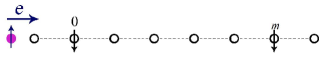
Figure 1: Scattering of a free traveling electron by two on-site spin impurities localized at a distance of $m$ from each other in a one-dimensional tight-binding chain.

Without loss of generality, it is assumed that the impurities are localized at sites $0$ and $m$, respectively. So, the Hamiltonian of the system reads

$$H=\sum_{i}tc^{\dagger}_{i}c_{i+1}+hc+{\hat{V}},$$ (1)

where summation runs over all lattice sites and $hc$ stands for Hermitian conjugate. $t$ is the hopping integral between nearest neighbors, $c^{\dagger}_{i}~{}(c_{i})$ is the creation (annihilation) operator of an electron at site $i$ and ${\hat{V}}$ is the interaction potential due to the presence of the impurities.

In the face of the impurities, the electron matter wave is partially reflected and transmitted. The reflection and transmission amplitudes can be evaluated using the so-called transition matrix approach. For a typical scattering potential of ${\hat{V}}$, the transition operator ${\hat{T}}$ is defined as

$$\hat{T}=\hat{V}\big{(}1+\hat{G}_{E}\hat{V}+\hat{G}_{E}\hat{V}\hat{G}_{E}\hat{V}+...\big{)}=\hat{V}\big{(}1-\hat{G}_{E}\hat{V}\big{)}^{-1},$$ (2)

where $\hat{G}_{E}$ is the Green’s operator of the defect-free system. Here, both $\hat{T}$ and $\hat{G}_{E}$ are dependent on the energy of the system, $E$, but for brevity we refuse to display it explicitly.

For a one-dimensional tightly bonded system the matrix elements of $\hat{G}_{E}$ in the site basis are given by a closed-form expression as Economou1990 :

$$G_{E}(m;m^{\prime})=\langle m|\hat{G}_{E}|m^{\prime}\rangle={e^{ik_{0}|m-m^{\prime}|}\over 2it\sin k_{0}},$$ (3)

in which $m$ and $m^{\prime}$ are the numbers labeling the sites and their corresponding basis $|m\rangle$ and $|m^{\prime}\rangle$ are obtained by acting the creation operators $c^{\dagger}_{m}$ and $c^{\dagger}_{m^{\prime}}$ on the vacuum ground state. Also $k_{0}$ is given by $k_{0}=\cos^{-1}(E/2t)$.

The scattering potential $\hat{V}$, due to the presence of the doped spin impurities in the lattice, is in explicit form of

$$\hat{V}=U\big{[}({\bf S}_{1}\cdot{\bf S}_{2})c_{0}^{\dagger}c_{0}+({\bf S}_{1}\cdot{\bf S}_{3})c^{\dagger}_{m}c_{m}\big{]},$$ (4)

${\bf S}_{1}$ is the dimensionless spin operator of the incident electron, ${\bf S}_{2}$ and ${\bf S}_{3}$ are the same for the impurities, and $U$ is the impurity potential in the system.

In a representation space including the involved spins as well as the site states $|0\rangle$ and $|m\rangle$, this potential can be represented as a squared $16\times 16$ matrix, while the spin interactions are $4\times 4$ matrices in their corresponding subspaces. For example, in the computational basis the spin interaction ${\bf S}_{1}\cdot{\bf S}_{2}$ is given by

$${\bf S}_{1}\cdot{\bf S}_{2}={1\over 4}|t\rangle\langle t|-{3\over 4}|s\rangle\langle s|$$ (5)

where $t$ and $s$ refer to triplet (symmetric) and singlet (asymmetric) spin states, respectively. Clearly, the explicit matrix form of this interaction is

$${\bf S}_{1}\cdot{\bf S}_{2}=\begin{bmatrix}{1\over 4}&0&0&0\\ 0&-{1\over 4}&\ \ {1\over 2}&0\\ 0&\ \ {1\over 2}&-{1\over 4}&0\\ 0&0&0&{1\over 4}\end{bmatrix}.$$ (6)

A similar matrix form can be derived for the other spin interaction, ${\bf S}_{1}\cdot{\bf S}_{3}$. Consequently, the interaction potential cab be written as

$$\hat{V}=U\big{[}({\bf S}_{1}\cdot{\bf S}_{2}\big{)}_{4\times 4}\otimes{\bf 1}_{3}\otimes|0\rangle\langle 0|+\big{(}{\bf S}_{1}\cdot{\bf S}_{3}\big{)}_{4\times 4}\otimes{\bf 1}_{2}\otimes|m\rangle\langle m|\big{]},$$ (7)

where ${\bf 1}_{2}$ and ${\bf 1}_{3}$ are the identity matrices on the spin spaces of the impurities and $|0\rangle\langle 0|$ and $|m\rangle\langle m|$ are the on-site projection operators . The interaction operator can be also rewritten in a more compact form of

$$\hat{V}={\hat{V}}_{00}\otimes|0\rangle\langle 0|+{\hat{V}}_{mm}\otimes|m\rangle\langle m|,$$ (8)

with

$$\begin{split}{\hat{V}}_{00}=\big{(}V_{00}\big{)}_{8\times 8}&=U({\bf S}_{1}\cdot{\bf S}_{2}\big{)}_{4\times 4}\otimes{\bf 1}_{3},\\ {\hat{V}}_{mm}=\big{(}V_{mm}\big{)}_{8\times 8}&=U\big{(}{\bf S}_{1}\cdot{\bf S}_{3}\big{)}_{4\times 4}\otimes{\bf 1}_{2}.\end{split}$$ (9)

Using this form of the interaction potential, it is an easy practice to show that transition matrix $\hat{T}$, given in Eq. (2), can be represented as

$$\hat{T}={\hat{V}}\big{(}1-\hat{\chi}\big{)}^{-1},$$ (10)

where $\hat{\chi}$ is a 16-dimensional square matrix of the following form

$${\hat{\chi}}=\begin{bmatrix}\hat{G}_{00}&\hat{G}_{0m}\\ \hat{G}_{m0}&\hat{G}_{mm}\end{bmatrix}\,\begin{bmatrix}\hat{V}_{00}&0\\ 0&\hat{V}_{mm}\end{bmatrix}.$$ (11)

In the above equation, matrix block $\hat{G}_{mm^{\prime}}$ reads $\hat{G}_{mm^{\prime}}=G_{E}(m;m^{\prime})~{}{\bf 1}_{spin}$, where $G_{E}(m;m^{\prime})$ is given in Eq. (3) and identity operator ${\bf 1}_{spin}$ reads ${\bf 1}_{spin}={\bf 1}_{1}\otimes{\bf 1}_{2}\otimes{\bf 1}_{3}$.

As is known, the direct spin (electron-impurity) interaction can be modeled as a short range Heisenberg exchange. Accordingly, we consider the spatial and spinorial spaces in an incoming wave stat of $|\Psi_{in}\rangle$ with a wave number of $k_{0}$ for instance as $|\Psi_{in}\rangle=\sum\limits_{m}e^{ik_{0}m}|m\rangle|\uparrow\downarrow\downarrow\rangle$. In the initial wave state, it is assumed that the incident electron has initially spin up while both impurities have spin down in the $z$ direction.

The outgoing wave state, $|\Psi_{out}\rangle$, can be obtained as a solution of the Lippmann-Schwinger equation

$$\begin{split}|\Psi_{out}\rangle&=\big{[}1+\hat{G}_{E}\hat{T}\big{]}|\Psi_{in}\rangle\\ &=\big{[}1+{\hat{G}}_{E}{\hat{V}}\big{(}1-\hat{\chi}\big{)}^{-1}\big{]}|\Psi_{in}\rangle\\ &=|\Psi_{in}\rangle+\hat{G}_{E}|\Psi^{\prime}\rangle,\end{split}$$ (12)

in which the auxiliary wave state $|\Psi^{\prime}\rangle$ is defined as $|\Psi^{\prime}\rangle={\hat{V}}\big{(}1-\hat{\chi}\big{)}^{-1}|\Psi_{in}\rangle$. Considering the matrix form of the interaction potential, $\hat{V}$, and the transition matrix, $\hat{T}$, it is obvious that $|\Psi^{\prime}\rangle$ has a general form of

$$|\Psi^{\prime}\rangle=|s_{0}\rangle|0\rangle+|s_{m}\rangle|m\rangle,$$ (13)

where $|s_{0}\rangle$ and $|s_{m}\rangle$ are two total spin states which are derivable analytically.

Two parts are included in the outgoing state, the reflected part $|\Psi_{R}\rangle$ which is detectable at the left side of the impurities, and the transmitted part, $|\Psi_{T}\rangle$, detectable at those right side. Using Eqs. (12) and (13), the reflected and transmitted wave states are derivable in the final form of

$$\begin{split}|\Psi_{R}\rangle&=e^{-ik_{0}m^{\prime}}|S_{R}\rangle|m^{\prime}\rangle;\qquad{\rm~{}for}\ m^{\prime}<0,\\ |\Psi_{T}\rangle&=e^{+ik_{0}m^{\prime}}|S_{T}\rangle|m^{\prime}\rangle;\qquad{\rm~{}for}\ m^{\prime}>m,\\ \end{split}$$ (14)

where the reflected and transmitted spin states, $|S_{R}\rangle$ and $|S_{T}\rangle$ are

$$\begin{split}|S_{R}\rangle&=[G_{m^{\prime}0}|s_{0}\rangle+G_{m^{\prime}m}|s_{m}\rangle]e^{+ik_{0}m^{\prime}},\\ |S_{T}\rangle&=|\uparrow\downarrow\downarrow\rangle+[G_{m^{\prime}0}|s_{0}\rangle+G_{m^{\prime}m}|s_{m}\rangle]e^{-ik_{0}m^{\prime}}.\end{split}$$ (15)

The reflection, transmission and total partial density matrices, $\rho_{23R}$, $\rho_{23T}$, and $\rho_{23}$ are defined as

$$\begin{split}\rho_{23R}&=Tr_{1}\big{(}|S_{R}\rangle\langle S_{R}|\big{)}~{}/~{}Tr\big{(}|S_{R}\rangle\langle S_{R}|\big{)},\\ \rho_{23T}&=Tr_{1}\big{(}|S_{T}\rangle\langle S_{T}|\big{)}~{}/~{}Tr\big{(}|S_{T}\rangle\langle S_{T}|\big{)},\\ \rho_{23}&=\rho_{23R}+\rho_{23T},\end{split}$$ (16)

where $Tr_{1}(A)$ stands for the trace of $A$ over the electron spin degree of freedom. These partial density matrices can be used to evaluate the amount of the created entanglement between the doped impurities. Also, the reflection and transmission probabilities can be evaluated using the above quantum states. These issues will be further discussed in the Results section.

III entanglement generation in a zigzag phosphorene nanoribbon

In this section, the phosphorene edge states in a zigzag nanoribbon are introduced and their corresponding Green’s function is analytically derived. Scattering of electrons from two on-side spin impurities doped to the zigzag edges of a phosphorene nanoribbon is considered. The introduced edge states are used to describe the incident electrons and the derived Green’s function is used to evaluate the amount of the produced entanglement between the impurities. As will be seen, the approach is very similar to what was followed in the previous section.

An impurity-doped infinite zPNR of a given width is schematically shown in Fig. 2. As is seen, the unit cell contains two atoms labeled $A$ and $B$. The electronic structure of this lattice is described by a tight-binding Hamiltonian as

$${\hat{H}}={\hat{H}}_{0}+{\hat{V}}=\sum_{\langle i,j\rangle}t_{ij}c_{i}^{\dagger}c_{j}+hc+{\hat{V}},$$ (17)

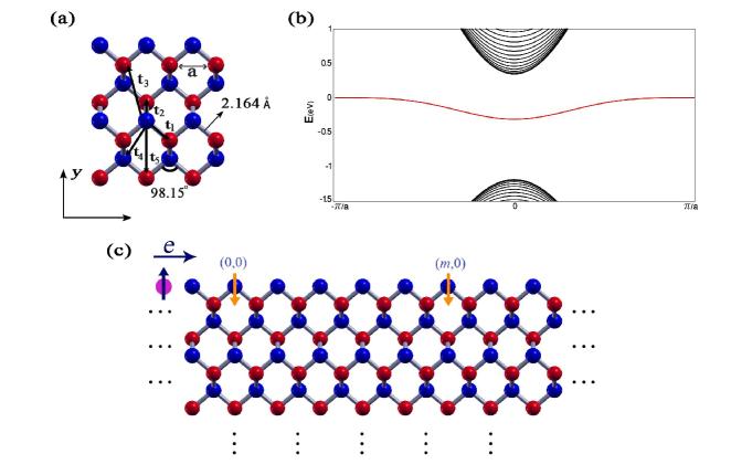
Figure 2: (Color online) (a) Schematic of the lattice structure of phosphorene and hopping integrals $t_{i}$, blue (A) and red (B) colors refer to two types of atoms in the lattice, (b) band structure of a phosphorene nanoribbon: there is a considerable gap between the conduction and valence bands and the degenerate quasi-flat bands occur separately at the middle of this gap, (c) Scattering of the edge-state electrons from the impurities on two sites of the zigzag edge of a phosphorene nanoribbon, the sites are labeled as $(0,0)$ and $(m,0)$.

where $\langle i,j\rangle$ stands for the nearest-neighbor index, $c^{\dagger}_{i}~{}(c_{i})$ is the same as introduced previously, $t_{ij}$ is the hopping integral between sites $i$ and $j$, and ${\hat{V}}$ is the Hamiltonian due to the presence of the impurity.

Using the ab initio method Rudenko2014 , it has been shown that only five hopping parameters are sufficient to describe the band structure of phosphorene. Referring to Fig. 2, we indicate these parameters for simplicity by $t_{1}$ to $t_{5}$. The corresponding values for these parameters are $t_{1}=-1.220~{}eV$, $t_{2}=3.665~{}eV$, $t_{3}=-0.205~{}eV$, $t_{4}=-0.105~{}eV$, and $t_{5}=-0.055~{}eV$. The interaction term including $t_{4}$ causes the particle-hole symmetry breaking in the lattice and it should be kept in the further simplifications. But, in comparison with $t_{1}$ and $t_{2}$, it will be a good approximation if one neglects the smaller values of $t_{3}$ and $t_{5}$.

Accordingly, an effective anisotropic honeycomb lattice model was developed Ezawa2014 to analytically describe the electronic structure of phosphorene. In that model, the terms including $t_{1}$ and $t_{2}$ was considered as the tight-binding Hamiltonian with exact solutions while the interaction including $t_{4}$ was handled as a perturbation.

The band structure of a phosphorene nanoribbon is shown in Figure 2. A remarkable feature of a zPNR confined system is the presence of the quasi-flat edge bands isolated from the bulk modes. As is seen in 2 these degenerate quasi-flat bands in the middle of the conduction-valence gap entirely detached from the bulk band. Adopting the above mentioned model, considering the term including $t_{4}$ as a perturbation, the exact corresponding wave function of such quasi-flat edge modes on an edge formed of atoms A, can be written as Ezawa2014

$$|\Psi^{A}_{k}\rangle={1\over\sqrt{2\pi}}\sum_{m,n}\alpha^{n}(k)\gamma(k)e^{ik(m+\delta_{n})}|m,n\rangle.$$ (18)

where $k$ is the wave-number. Here, without loss of generality, we continue the discussion by considering an edge formed of $A$ atoms and remark that the wave state on the sites of B atoms is zero.

In Eq. (18), each lattice site is labeled by a pair of integers $(m,n)$, where $m$ and $n$ are armchair and zigzag chain numbers. It is assumed that for the considered edge $n=0$.

The value of $\delta_{n}$ in Eq. (18) is 0 (0.5) for even (odd) $n$, $\alpha(k)=-2\big{(}t_{1}/t_{2}\big{)}\cos(k/2)$, and normalization factor $\gamma(k)$ satisfies the equation $\gamma^{2}(k)=1-\alpha^{2}(k)$.

It is obvious that the exact energy corresponding to the eigenstate given in Eq. (18) is zero. In a first-order approximation, considering the perturbation interaction, it is straightforward to show that eigenenergy corresponding to the above edge state changes to Ezawa2014

$$\begin{split}E_{k}&=-4\big{(}t_{1}t_{4}/t_{2}\big{)}\big{[}1+\cos k\big{]}\\ &=E_{0}-2t^{\prime}\cos{k},\end{split}$$ (19)

where $E_{0}=-2t^{\prime}=-4t_{1}t_{4}/t_{2}$ is an energy shift. As is seen, energy shifts toward the negative values and the obtained dispersion is very similar to what happens for a one-dimensional tight-binding chain.

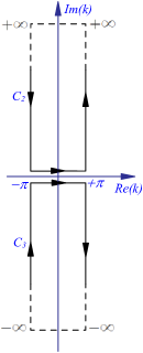
Figure 3: (Color online) The integration contours in complex plane used to derive the closed forms of the diagonal matrix elements of Green operator ${\hat{G}}_{E}$, $C_{2}$ is used for $I_{2}$ and $C_{3}$ for $I_{3}$.

III.1 zPNR Green’s function

Scattering of the edge states by impurities is one of the main issues to study in this section. To this end, since there exists a considerable energy gap between the edge and bulk states, we need only the Green function of the edge states in their energy domain. The Green function corresponding to the edge states in zPNR can be expressed in terms of the eigenstates $|\Psi_{k}^{A}\rangle$ and eigenenergies $E_{k}$, respectively given in Eqs. (18) and (19), as

$$\hat{G}_{E}=\int_{-\pi}^{\pi}dk{|\Psi_{k}^{A}\rangle\langle\Psi_{k}^{A}|\over E-E_{k}+i0^{+}}.$$ (20)

The matrix elements of $\hat{G}_{E}$ can be evaluated as follows

$$\begin{split}G_{E}(m,n;m^{\prime},n^{\prime})&=\langle m,n|\hat{G}_{E}|m^{\prime},n^{\prime}\rangle\\ ={1\over 2\pi}\int_{-\pi}^{\pi}dk&{e^{-i(m-m^{\prime}+\delta_{n}-\delta_{n}^{\prime})}\alpha^{n+n^{\prime}}(k)\gamma^{2}(k)\over E-E_{0}+2t^{\prime}\cos k+i0^{+}}.\end{split}$$ (21)

The typical integrals appearing in the above equation can be evaluated by means of the residue theorem. For example, the diagonal element of $m=n=m^{\prime}=n^{\prime}=0$ can be easily separated into two terms as

$$G_{E}(0,0;0,0)=[1-2(t_{1}/t_{2})^{2}]I_{1}-(t_{1}/t_{2})^{2}(I_{2}+I_{3}),$$ (22)

where

$$\begin{split}I_{1}&={1\over 2\pi}\int_{-\pi}^{\pi}dk{1\over E-E_{0}+2t^{\prime}\cos k+i0^{+}},\\ I_{2}&={1\over 2\pi}\int_{-\pi}^{\pi}dk{e^{ik}\over E-E_{0}+2t^{\prime}\cos k+i0^{+}},\\ I_{3}&={1\over 2\pi}\int_{-\pi}^{\pi}dk{e^{-ik}\over E-E_{0}+2t^{\prime}\cos k+i0^{+}}.\end{split}$$ (23)

For the first integral, $I_{1}$, we can use the variable change of $z=e^{ik}$ to set $\cos k=(z+z^{-1})/2$ and $dk=idz/z$. By doing so, the denominator appears in the form of a second-order expression in terms of $z$ with two solutions. These solutions are the simple poles of the integrand. By closing the integration contour with a unit radius circle around the origin of the complex plane, only one of the poles occurs inside the contour. Employing the residue theorem, the derivation results in

$$I_{1}={1/2it^{\prime}\sin k_{0}},$$ (24)

where $\cos k_{0}=(E-E_{0})/2t^{\prime}$.

The integrand in $I_{2}$ has two simple poles at $k_{1}=k_{0}+i0^{+}$ and $k_{2}=-k_{0}-i0^{+}$ where $k_{0}=\cos^{-1}[(E-E_{0})/2t^{\prime}]$ with the same residues of $e^{+ik_{0}}/2t^{\prime}\sin k_{0}$. In order to perform the integral, we complete the integration contour by an infinite rectangle in the upper half-plane as shown in Fig. 3. The integrand over this contour vanishes as $Im(k)\to+\infty$. Also the contribution of the vertical paths to the integral is zero for the periodicity of the integrand. In this case, point $k_{1}$ is within and $k_{2}$ is exterior to the contour. Consequently, the final result for $I_{2}$ is

$$I_{2}=e^{+ik_{0}}/2it^{\prime}\sin k_{0}.$$ (25)

Proceeding in a similar manner, we may also derive an analytical form for $I_{3}$. In this case, since the exponential in the integrand is negative, the contour should be completed by an infinite rectangle in the lower half-plane as shown in Fig. 3. In this case, the integral vanishes as $Im(k)\to-\infty$ and only $k_{2}$ occurs inside the contour. Given these points, the result is as expected equal to what we obtained for $I_{2}$.

The substitution of the derived closed-form expressions for $I_{1}$, $I_{2}$ and $I_{3}$ into Eq. (22) leads to

$$G_{E}(0,0;0,0)={\gamma^{2}(k_{0})\over 2it^{\prime}\sin k_{0}}-{\big{(}{t_{1}/t_{2}}\big{)}^{2}\over 4t^{\prime}}.$$ (26)

Following the same analysis, it is straightforward to obtain the analytical form of the off-diagonal element $G_{E}(m,0;0,0)$ as

$$G_{E}(m,0;0,0)={\gamma^{2}(k_{0})e^{ik_{0}m}\over 2it^{\prime}\sin k_{0}}.$$ (27)

The derived expressions (26) and (27) will be used to study the scattering-induced entanglement in a zPNR.

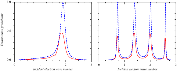
Figure 4: (Color online) Transmission probability as a function of the incident electron wave number for scattering from two spin impurities doped into two sites of a one-dimensional tight-binding chain. Solid (red) and dashed (blue) lines are respectively for the initial states of $|\uparrow\downarrow\downarrow\rangle$ and $|\uparrow\uparrow\uparrow\rangle$. The left (right) panel is for $m=2~{}(m=5)$. For all the cases U’=10.

III.2 Impurity entanglement through electron scattering

In this subsection, we assume that two spin impurities are doped into two edge sites of an $A$-type zigzag chain of a phosphorene nanoribbon. The edge-sate electrons traveling along the zigzag chain scatter off the impurities. We will show that the spin interaction between the incident electrons and the impurities during the scattering process causes the entanglement of the final spin state of the specified system. As is understood from the above subsections and also is seen in figure 4, the situation is very similar to what we discussed for a one-dimensional tight-binding chain in section II. In this case, by labeling the impurity sites by $(0,0)$ and $(m,0)$, the explicit form of the interaction due to their presence is

$$\hat{V}=U\big{[}({\bf S}_{1}\cdot{\bf S}_{2})c_{0,0}^{\dagger}c_{0,0}+({\bf S}_{1}\cdot{\bf S}_{3})c^{\dagger}_{m,0}c_{m,0}\big{]},$$ (28)

where $c_{0,0}^{\dagger}$ and $c^{\dagger}_{m,0}$ ($c_{0,0}$ and $c_{m,0}$) are the creation (annihilation) operators of electrons in sites $(0,0)$ and $(m,0)$, respectively, and the other quantities are the same as introduced previously. The incoming state is assumed for example as

$$|\Psi_{in}\rangle=|\Psi_{k}^{A}\rangle|\uparrow\downarrow\downarrow\rangle.$$ (29)

Using the Lippmann Schwinger equation and following the approach explained in section II, the reflected and transmitted wave states are respectively given by

$$|\Psi_{R}\rangle=|\Psi_{-k}^{A}\rangle|S_{R}\rangle;\qquad{\rm~{}for}\ m^{\prime}<0,$$ (30)

and

$$|\Psi_{T}\rangle=|\Psi_{k}^{A}\rangle|S_{T}\rangle;\qquad{\rm~{}for}\ m^{\prime}>m,$$ (31)

with the reflected and transmitted spin states of

$$\begin{split}|S_{R}\rangle&=[G_{E}(m^{\prime},0;0,0)|s_{0}\rangle\\ &\hskip 34.1433pt+G_{E}(m^{\prime},0;m,0)|s_{m}\rangle]e^{+ik_{0}m^{\prime}},\\ |S_{T}\rangle&=|\uparrow\downarrow\downarrow\rangle+[G_{E}(m^{\prime},0;0,0)|s_{0}\rangle\\ &\hskip 34.1433pt+G_{E}(m^{\prime},0;m,0)|s_{m}\rangle]e^{-ik_{0}m^{\prime}}.\end{split}$$ (32)

Here, also similar to the one-dimensional case discussed in section II, the total spin states of $|s_{0}\rangle$ and $|s_{m}\rangle$ are exactly known and their explicit forms can be derived analytically.

The wave states given in equations (29) and (30) can be used to the obtain the relevant partial density matrices and those in turn may be used to calculate the negativity as a measure of the produced entanglement in the final spin state of the system. Also, the reflection and transmission probabilities are computable using the above quantum states.

The calculations in this and previous sections can be repeated for any given initial spin state.

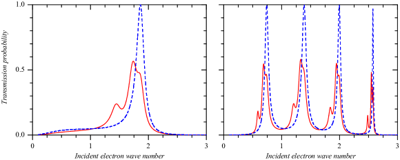
Figure 5: Same as figure 4, but for scattering of the edge-state electrons from two impurities doped into two sites of an A-type zPNR.

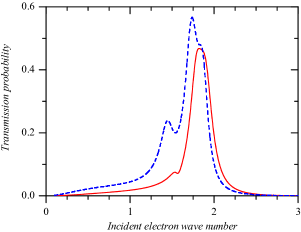
Figure 6: Comparison of the transmission probabilities for scattering of free electrons from impurities doped into two sites of a one dimensional chain (solid line) and scattering of the edge-state electrons from a zigzag chain in a phosphorene nanoribbon (dashed line). For both cases the initial spin state is $|\uparrow\downarrow\downarrow\rangle$, $m=0$ and $U^{\prime}=10$.

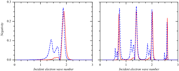
Figure 7: Negativity vs the incident electron wave number as a measure of the created entanglement due to the scattering of the free (edge-state) electrons from two spin impurities doped into two sites of a one-dimensional tight-binding chain (an edge zigzag chain of phospherene). Solid (red) and dashed (blue) lines are respectively for chain and phosphorene. The initial spin state in all the cases is $|\uparrow\downarrow\downarrow\rangle$. The left (right) panel is for $m=2~{}(m=5)$. For all the cases $U^{\prime}=10$.

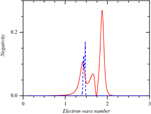
Figure 8: The created entanglement between two on-side magnetic impurities in an edge zigzag chain of phosphorene nanoribbon as a function of the incident electrons wave number. The initial state is $|\uparrow\downarrow\downarrow\rangle$, $m=2$, but $U^{\prime}=10$ (solid line) and $U^{\prime}=100$ (dashed line).

IV Results

In this section, in order to demonstrate the performance of the models discussed in the previous sections, several examples of the electron scattering-induced entanglement between the doped magnetic impurities are presented and discussed. In following discussions, it is assumed that the impurities are localized at sites labeled by $0$ and $m$ in a one-dimensional tightly bonded chain, and at sites $(0,0)$ and $(m,0)$ in the edge zigzag chain of a phosphorene nanoribbon. So, with $m$, the second impurity location is completely known in the both cases. Also, the strength of the scattering potential, $U$, is normalized to $U^{\prime}$, where $U^{\prime}=U/t$ for chain and $U^{\prime}=U/t^{\prime}$ for phosphorene with $t^{\prime}=2t_{1}t_{4}/t_{2}$.

Figure 4 presents the electron transmission probability for scattering of free traveling electrons along a one-dimensional tight-binding chain. The incident electrons scatter off two localized impurities at sites $0$ and $m$. The results are shown for $m=2$ and $m=5$ with initial spin states of $|\uparrow\downarrow\downarrow\rangle$ and $|\uparrow\uparrow\uparrow\rangle$. Strength of the normalized scattering potential, $U^{\prime}$, is set equal to 10.

As is seen from the figure, for the initial spin state in which all the three spins are in same direction, the behavior of the transmission probability is similar to what happens for scattering due to the on-site spinless interactions. In this case, for several values of the incident electron wave numbers, resonance occurs. The number of the resonance peaks are $m-1$ and their hight are equal to unit. With changing $U^{\prime}$ the number of the resonance peaks and their hight remain unchanged.

Also, for the initial spin state of $|\uparrow\downarrow\downarrow\rangle$, in which one of the spins is in opposite direction of the others, several resonance peaks are observed in the transition probability, but the hight of the peaks are smaller than that of the corresponding peaks for $|\uparrow\uparrow\uparrow\rangle$. For the initial spin state of $|\uparrow\downarrow\downarrow\rangle$, the electron transmission probability is a bit dependent on $U^{\prime}$ value.

A similar situation is investigated for scattering of the edge-state electrons from two on-site doped impurities into a A-type edge zigzag chain in a phosphorene nanoribbon. For this case, the changes of the electron transmission probability in terms of the incident electron wave number are presented in Fig. 5. As is seen from the figure, the behavior exhibited in this case is similar to what was observed for scattering from a one-dimensional chain. For the initial spin state with three spins in the same direction, the hight of the resonance peaks is unit but for other initial spin states this hight reduces considerably. The number of the resonance peaks in this case is also $m-1$. These facts confirm our assertion that the zigzag edge chains in phosphorene nanoribbons behaves like a one-dimensional tight-binding chain.

In figure 6, the changes of the electron transmission probabilities in terms of the the incident electron wave number for scattering of the free traveling electrons from the impurities in a one-dimensional tight-binding chain and for scattering of edge-state traveling electrons from the impurities in a phosphorene zigzag chain are compared. For both considered cases, $m=2$, $U^{\prime}=10$ and the initial spin state is assumed as $|\uparrow\downarrow\downarrow\rangle$. As is seen the graphs are very similar in overall futures, but the resonance peak for phosphorene is a little higher than that for chain. This is for the fact that the impurities in phosphorene are fixed on the edge sites, while the edge-state wave function slightly penetrates into the bulk.

The electron scattering leads to entanglement production between the spin impurities in the both specified cases. Negativity obtained using the partial density matrix $\rho_{23}$ is a measure of the produced entanglement. This measure is displayed as a function of the electron wave number in Fig. 7, for scattering of electrons in a chain and in a phosphorene nanoribbon. For all the cases, the initial state is $|\uparrow\downarrow\downarrow\rangle$ and $U^{\prime}=10$. The results are shown for $m=2$ and $m=5$.

Several points are remarkable from this figure. The resonance peaks are observable for the produced entanglement. In addition to the main resonance peaks, a number of the local small peaks are also seen in the resonance spectrum of the created correlation. Structure of these local peaks for phosphorene is more complex than that for chain, also these peaks for phosphorene are considerably higher than those of chain. This is for the fact that the edge-state wave function for phosphorene is more complicated than the considered wave function for chain. As previous, the number of the main resonance peaks is $m-1$ for both chain and nanoribbon. Overall aspects of the main peaks in phosphorene are similar to those in chain, however the phosphorene main peaks are usually a little higher than those of chain. In the resonance case the negativity tends to the considerable value of 0.3. This shows that the present model is very efficient in producing a considerable amount of entanglement.

In figure 8, we investigated the dependence of the created entanglement between the on-side impurities in the phosphorene nanoribbon on the normalized strength of the interaction potential $U^{\prime}$. To this end, the negativity is plotted as a function of the incident electron wave number for two values of $U^{\prime}$; $U^{\prime}=10$ and $U^{\prime}=100$. As is seen, with increasing $U^{\prime}$, the local peaks disappear and the main peaks becomes more sharper but their hight decreases. A similar behavior is also observable for the electron transmission probability. In fact, the increase in $U^{\prime}$ causes that the electron transmission probability becomes considerable only at certain specific resonance energies. As a result the produced entanglement between the impurities is significant only at theses resonance situations.

V Summary and Conclusions

We studied the scattering of the edge-state electrons, traveling along an edge zigzag chain of a phosphorene nanoribbon, from two magnetic impurities localized at two sites of this chain. It was shown that the situation is very similar to the scattering of free traveling electrons from a one-dimensional tight-binding chain with two on-side spin impurities. With a given initial wave state, the Lippmann-Schwinger equation, the tight-binding model and the Green’s function approach were employed to calculate the outgoing wave state, analytically. Using the provided model, the reflected and transmitted parts of the final wave state and their relevant partial density matrices were derived. Consequently, the reflection, and transmission probabilities and the negativity as a measure of the created entanglement between the impurities were calculated. Several examples were presented and discussed to show the performance of the suggested model. It was shown that, for certain resonance energies, both the electron transmission probability and the generated correlation between the magnetic impurities are considerable. The importance of the performed research is that it proposed a method for creating the entanglement between two magnetic impurities, which possibly can be realized using the experimental methods.

- (1) H. Liu, A. T. Neal, Z. Zhu, Z. Luo, X. Xu, D. Tomanek, and P. D. Ye, ACS Nano 8, 4033 (2014).
- (2) Alexandra Carvalho, Min Wang, Xi Zhu, Aleksandr S. Rodin, Haibin Su and Antonio H. Castro Neto, Nat. Rev. Mater. 1, 16061 (2016).
- (3) X. Ling, H. Wang, S. Huang, F. Xia, and M. S. Dresselhaus, Proc. Natl. Acad. Sci. (USA) 112, 4523 (2015).
- (4) A. S. Rodin, A. Carvalho, and A. H. Castro Neto, Phys. Rev. Lett. 112, 176801 (2014).
- (5) J. Qiao, X. Kong, Z. X. Hu, F. Yang, and W. Ji, Nat. Commun. 5, 4475 (2014).
- (6) D. Cakir, H. Sahin, and F. M. Peeters, Phys. Rev. B 90, 205421 (2014).
- (7) T. Low, R. Roldan, H. Wang, F. Xia, P. Avouris, L. M. Moreno, and F. Guinea, Phys. Rev. Lett. 113, 106802 (2014).
- (8) R. Fei and L. Yang, Nano Lett. 14, 2884 (2014).
- (9) S. Yuan, A. N. Rudenko, and M. I. Katsnelson, Phys. Rev. B 91, 115436 (2015).
- (10) M. Elahi, K. Khaliji, S.M. Tabatabaei, M. Pourfath and R. Asgari, Phys. Rev. B 91, 115412 (2015).
- (11) Qingyun Wu, Lei Shen, Ming Yang, Yongqing Cai, Zhigao Huang, and Yuan Ping Feng, Phys. Rev. B 92, 035436 (2015).
- (12) Ajanta Maity, Akansha Singh, Prasenji Sen, Aniruddha Kibey,Anjali Kshirsagar, and Dilip G. Kanhere, Phys. Rev. B 94, 075422 (2016).
- (13) Fang Xie, Zhi-Qiang Fan, Xiao-Jiao Zhang, Jian-Ping Liu, Hai-Yan Wang,Kun Liu, Ji-Hai Yu, Meng-Qiu Long, Organic Electronics 42, 21 (2017).
- (14) M. Ezawa, New Journal of Physics 16, 115004 (2014).
- (15) Z. Nourbakhsh and R. Asgari, arXiv:1803.00751(2018).
- (16) E. Ghanbari-Adivi, M. Soltani, and H. Ebtekarnasab, Eur. Phys. J. D 67, 118 (2013)
- (17) E. Ghanbari-Adivi, M. Soltani, and M. N. Sheikhali, Eur. Phys. J. D 69, 172 (2015)
- (18) E. Ghanbari-Adivi, M. Soltani, and M. Sheikhali, Quantum Inf. Process. 15, 2377 (2016)
- (19) E. N. Economou, Green’s function in quantum physics, Springer Verlag, Berlin (2006)
- (20) A. N. Rudenko, M. I. Katsnelson, Phys. Rev. B 89, 201408 (2014).