Convexity and Operational Interpretation of the
Quantum Information Bottleneck Function

Abstract

In classical information theory, the information bottleneck method (IBM) can be regarded as a method of lossy data compression which focusses on preserving meaningful (or relevant) information. As such it has of late gained a lot of attention, primarily for its applications in machine learning and neural networks. A quantum analogue of the IBM has recently been defined, and an attempt at providing an operational interpretation of the so-called quantum IB function as an optimal rate of an information-theoretic task, has recently been made by Salek et al. The interpretation given by these authors is however incomplete, as its proof is based on the conjecture that the quantum IB function is convex. Our first contribution is the proof of this conjecture.

Secondly, the expression for the rate function involves certain entropic quantities which occur explicitly in the very definition of the underlying information-theoretic task, thus making the latter somewhat contrived. We overcome this drawback by pointing out an alternative operational interpretation of it as the optimal rate of a bona fide information-theoretic task, namely that of quantum source coding with quantum side information at the decoder, which has recently been solved by Hsieh and Watanabe. We show that the quantum IB function characterizes the rate region of this task,

We similarly show that the related privacy funnel function is concave (both in the classical and quantum case). However, we comment that it is unlikely that the quantum privacy funnel function can characterize the optimal asymptotic rate of an information theoretic task, since even its classical version lacks a certain essential additivity property.

I Introduction

Consider a given pair of random variables $(X,Y)$ with joint probability distribution $p_{XY}$. In this paper, all random variables are considered to be discrete, taking values $x,y$ in finite alphabets ${\mathcal{X}}$ and ${\mathcal{Y}}$, respectively. Tishby et al. [1] introduced the notion of the meaningful or relevant information that $X$ provides about $Y$. They formalized this notion as a constrained optimization problem of finding the optimal compression of $X$ (to a random variable $W$, say) which still retains maximum information about $Y$. The authors of [1] named this problem Information Bottleneck since $W$ can be viewed as the result of squeezing the information that $X$ provides about $Y$ through a “bottleneck”. The information bottleneck can be regarded as a problem of lossy data compression for a source defined by the random variable $X$, in presence of side information given by $Y$. The standard theory of lossy data compression introduced by Shannon [2] is rate distortion theory, which deals with the trade-off between the rate of lossy compression and the average distortion of the distorted signal (see also [3, 4]). The Information Bottleneck Method (IBM) can be considered as a generalization of this theory, in which the distortion measure between $X$ and $W$ is determined by the joint distribution $p_{XY}$. This method has found numerous applications, e.g. in investigating deep neural networks [5, 6], video processing [7], clustering [8] and polar coding [9].

The constraint in the above-mentioned optimization problem, is given as a lower bound, say $I_{Y}$, on the mutual information, $I(Y;W)=H(Y)+H(W)-H(YW)$, since the latter is a measure of the information about $Y$ contained in $W$. Here $H(Y)$ denotes the Shannon entropy of $Y$, i.e. if $Y$ has a probability mass function $\{p(y)\}_{y\in{\mathcal{Y}}}$, where ${{\mathcal{Y}}}$ is a finite alphabet, then $H(Y)=-\sum_{y\in{\mathcal{Y}}}p(y)\log p(y)$. The rate function of the IBM, the so-called IB function, is a function of this bound and is given by

$$R(I_{Y}) =\min_{p(w|x)\atop{I(Y;W)\geq I_{Y}}}I(X^{\prime};W),\quad{\hbox{for}}\ I_{Y}\geq 0,$$ (1)

where $X^{\prime}=X$, and the minimization is over the set of conditional probabilities $\{p(w|x)\}$, with $w$ denoting values taken by the random variable $W$.

A dual quantity, which gives an expression for the information $I_{Y}$ as a function of the rate $R$, is given by

$$I_{Y}(R) =\max_{p(w|x)\atop{I(X^{\prime};W)\leq R}}I(Y;W),\quad{\hbox{for}}\ R\geq 0.$$ (2)

It was shown in [10, Lemma 10] that the optimization problems in (1) and (2) are indeed dual to each other, meaning that $R(I_{Y})$ and $I_{Y}(R)$ are equivalent quantities, in the sense that they define the same curve with switched axes for $0\leq I_{Y}\leq I(W;Y)$ and $0\leq R\leq R(I(W;Y))$. In other words, $R$ and $I_{Y}$ are functions inverse to each other.

As a matter of fact, in [11], the following closely related optimization problem was investigated:

$$F(a)=\min_{\begin{subarray}{c}p(w|x)\\ H(X|W)\geq a\end{subarray}}H(Y|W),$$ (3)

where $H(Y|W):=H(YW)-H(W)$ is the conditional entropy. It was furthermore shown that $F(a)$ is always convex. It can easily be seen that $I_{Y}(a)=H(Y)-F(H(X)-a)$; it follows that $I_{Y}(R)$ is concave and $R(I_{Y})$ is convex.

Operational interpretation of the classical IB function

An operational interpretation of the IB function is obtained by considering the function $\widehat{F}(a)=H(Y)-I_{Y}(a)$. More precisely, its interpretation follows from that of $\widehat{F}(a)$ via the so-called Wyner-Ahlswede-Körner (WAK) problem [12, 13]. The setting considered for the WAK problem is that of source coding with side information at the decoder. In this paper we will be concerned with a generalization of this task to the quantum setting, so let us review the WAK problem briefly.

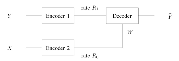
Figure 1: Schematic of the Wyner-Ahlswede-Körner problem.

The WAK problem concerns encoding information about one random variable such that it can be reconstructed using information about another (correlated) random variable. Let $X$ and $Y$ be two correlated random variables. One encodes $X$ and $Y$ separately, at rates $R_{0}$ and $R_{1}$, respectively. Both encodings are available to the decoder. A pair of rates $(R_{0},R_{1})$ is called achievable if it allows for exact reconstruction of $Y$ in the asymptotic i.i.d. setting. Since we do not aim to recover $X$, its encoding is considered as side information at the decoder provided by a helper. It was found independently in [12] and [13] that the minimal achievable rate $R_{1}$ under the constraint $R_{0}\leq a$ is given by $\widehat{F}(a)$.

II Quantum information bottleneck

A quantum generalization of the information bottleneck was first proposed by Grimsmo and Still [14]. They considered the following problem: let $\rho_{X}$ denote the state of a quantum system $X$, and let $\psi_{XR}$ denote its purification. The purifying reference system, $R$, is sent through a quantum channel, i.e. a linear completely positive trace-preserving (CPTP) map ${\mathcal{R}}:R\to Y$. It is only the information in $Y$ which is deemed important or relevant. The aim is to find an optimal encoding (i.e. compression) ${\mathcal{N}}:X\to M$ of $X$ into a quantum “memory” system $M$, which enables the retention of as much information about $Y$ as possible, without storing any unnecessary data. They quantified the information encoded about the initial data via the quantum mutual information $I(M;R)$, and the information available in $M$ about $Y$ by the quantum mutual information $I(M;Y)$. The optimal encoding is then the solution over an optimization problem in which $I(M;Y)$ is maximized over all possible channels, such that $I(M;R)$ is below a given threshold.

Formally, for a given bipartite quantum state $\rho_{XY}$, the quantum IB function, is defined through the following constrained optimization problem:

$$R_{q}(a) =\inf_{\operatorname{\mathcal{N}}^{X\to W}\atop{I(Y;W)_{\sigma}\geq a}}I(X^{\prime};W)_{\tilde{\tau}},\quad\text{for}\ a\geq 0,$$ (4)

where the optimization is over all linear CPTP maps $\operatorname{\mathcal{N}}^{X\to W}$ mapping states of $X$ to states of $W$, under the given constraint. In the above, ${\tilde{\tau}}_{X^{\prime}W}:=({\rm{id}}_{X^{\prime}}\otimes\operatorname{\mathcal{N}}^{X\to W})\tau_{X^{\prime}X}$, where $\tau_{X^{\prime}X}$ is a purification of $\rho_{X}$, and $\sigma_{WY}:=(\operatorname{\mathcal{N}}^{X\to W}\otimes{\rm{id}}_{Y})\rho_{XY}$. Hence $\rho_{X}=\operatorname{Tr}_{X^{\prime}}\tau_{X^{\prime}X}=\operatorname{Tr}_{Y}\rho_{XY}$. Here, $I(Y;W)_{\sigma}:=S(\sigma_{Y})+S(\sigma_{W})-S(\sigma_{YW})$ denotes the quantum mutual information, with $S(\sigma_{Y}):=-\operatorname{Tr}(\sigma_{Y}\log\sigma_{Y})$ being the von Neumann entropy.

However, the operational significance of this task remained unclear. Later, Salek et al. [15] attempted to give an operational interpretation to the quantum IB function. They showed that it is the optimal asymptotic rate of a certain information-theoretic task, under the assumption that the quantum IB function is convex. The task that they considered was the following constrained version of entanglement-assisted lossy data compression, in the communication paradigm, with a suitable choice of distortion measure. The state ($\rho_{X}$) to be compressed is in the possession of the sender (say, Alice), and is the reduced state of a bipartite state $\rho_{XY}$. Alice does not have access to the system $Y$. There is a noiseless classical channel between the her and the receiver (say, Bob). Alice and Bob also have prior shared entanglement. The relevant information that the state of the quantum system $X$ provides about that of $Y$ is quantified by the quantum mutual information $I(X;Y)_{\rho}$. Alice compresses $\rho_{X}$ and sends it through the noiseless classical channel to Bob, who then decompresses the data. Alice and Bob each use their share of entanglement in their respective compression and decompression tasks. The aim of the task is to find the optimal rate (in bits) of data compression under the constraint that the relevant information does not drop below a certain pre-assigned threshold.

We will complete Salek et al.’s work by showing in the following section that the quantum IB function is indeed convex, as they had conjectured.

At the same time, one might argue that the information-theoretic task considered is somewhat contrived, since it includes a constraint on an entropic function, namely a quantum mutual information, in its definition. Usually, the definition of an information-theoretic task is entirely operational, and the entropic quantities characterizing the optimal rates arise solely as a result of the computation. We will address this criticism by providing such an interpretation in section IV.

III Convexity of the QIB function

Our first result is the proof of the convexity of the quantum IB function, as conjectured in [15]. To do so, we start with the observation that the quantity $R_{q}(a)$ of Eq. (4) can be expressed equivalently as follows:

$$R_{q}(a) =\inf_{\operatorname{\mathcal{N}}^{X\to W}\atop{I(Y;W)_{\sigma}\geq a}}I(YR;W)_{\sigma},\quad\text{for}\ a\geq 0.$$ (5)

To see why, let $\psi_{XYR}$ be a purification of $\rho_{XY}$. Since it is also a purification of $\rho_{X}$, there must exist an isometry ${\mathcal{V}}:X^{\prime}\to YR$ such that

$$({\mathrm{id}}_{X}\otimes{\mathcal{V}}^{X^{\prime}\to YR})\tau_{XX^{\prime}}=\psi_{XYR}.$$ (6)

Then, defining $\sigma_{WYR}:=(\operatorname{\mathcal{N}}^{X\to W}\otimes{\mathrm{id}}_{YR})\psi_{XYR}$, by the invariance of the mutual information under isometries, and the fact that ${\tilde{\tau}}_{W}:=\operatorname{Tr}_{X^{\prime}}{\tilde{\tau}}_{X^{\prime}W}=\sigma_{W}$, with ${\tilde{\tau}}_{X^{\prime}W}$ defined as in Eq. (4), we have

$$I(X^{\prime};W)_{\tilde{\tau}}=I(YR;W)_{\sigma}.$$ (7)

The representation Eq. (5) has the benefit of referring to information quantities of the same tripartite state (rather than two different ones), both in the objective function and the optimization constraint.

Theorem 1

The quantum IB function $R_{q}(a)$ defined through Eq. (4), is convex, i.e.

$$R_{q}(\lambda a_{0}+(1-\lambda)a_{1}) \leq\lambda R_{q}(a_{0})+(1-\lambda)R_{q}(a_{1}),$$ (8)

for all $\lambda\in[0,1]$ and $a_{0},\,a_{1}\geq 0$.

Proof:

Let $\operatorname{\mathcal{N}}_{0}^{X\to W}$ and $\operatorname{\mathcal{N}}_{1}^{X\to W}$ be the optimizing channels in Eq. (5) for $a_{0}$ and $a_{1}$ respectively, such that $I(Y;W)_{\sigma_{0}}\geq a_{0}$ and $I(Y;W)_{\sigma_{1}}\geq a_{1}$, where for $i=0,1$,

$$\sigma_{i} =(\operatorname{\mathcal{N}}_{i}^{X\to W}\otimes{\mathrm{id}}_{YR})\psi_{XYR}.$$ (9)

Hence $R_{q}(a_{i})=I(YR;W)_{\sigma_{i}}$ for $i=0,1$. Next consider the flagged channel $\operatorname{\mathcal{N}}^{X\to WW^{\prime}}$, with a qubit $W^{\prime}$, defined as follows: for $\lambda\in[0,1]$, let

$$\operatorname{\mathcal{N}}^{X\to WW^{\prime}} :=\lambda\operatorname{\mathcal{N}}_{0}\otimes|0\rangle\!\langle 0|_{W^{\prime}}+\lambda\operatorname{\mathcal{N}}_{1}\otimes|1\rangle\!\langle 1|_{W^{\prime}},$$ (10)

Then $\sigma_{YRWW^{\prime}}:=(\operatorname{\mathcal{N}}^{X\to WW^{\prime}}\otimes{\mathrm{id}}_{YR})\psi_{XYR}$ is a block-diagonal state with diagonal blocks $\lambda\sigma_{0}^{WYR}$ and $(1-\lambda)\sigma_{1}^{WYR}$ respectively. Thus,

$$I(Y;WW^{\prime})_{\sigma} =\lambda I(Y;W)_{\sigma_{0}}+(1-\lambda)I(Y;W)_{\sigma_{1}}$$

$$\geq\lambda a_{0}+(1-\lambda)a_{1},\text{ and}$$ (11)

$$I(YR;WW^{\prime})_{\sigma} =\lambda I(YR;W)_{\sigma_{0}}+(1-\lambda)I(YR;W)_{\sigma_{1}}$$

$$=\lambda R_{q}(a_{0})+(1-\lambda)R_{q}(a_{1}).$$ (12)

Therefore,

$$R_{q}(\lambda a_{0}+(1-\lambda)a_{1})=\inf_{\operatorname{\mathcal{N}}^{X\to W}\atop{I(Y;W)\geq\lambda a_{0}+(1-\lambda)a_{1}}}I(YR;W)$$

$$\leq I(YR;WW^{\prime})_{\sigma}=\lambda R_{q}(a_{0})+(1-\lambda)R_{q}(a_{1}),$$ (13)

concluding the proof. ∎

This not only serves to complete the proof of the operational interpretation of the quantum IB function given in [15], but is also of independent interest.

IV Operational interpretation

We now show that the quantum IB function precisely characterizes the achievable rate region of a bona fide information theoretic task, namely, that of quantum source coding with quantum side information at the decoder [16], described below and summarized in Theorem 2.

The task: quantum Wyner-Ahlswede-Körner problem

Let us start by giving an explicit description of the task, which is a quantum version of the WAK problem, following the work of Hsieh and Watanabe [16]. It involves three parties Bob – the sender (or encoder), Charlie – the receiver (or decoder), and Alice – the helper. In contrast to the classical setting, one furthermore allows for prior shared entanglement between the helper and the decoder.

Suppose a source provides Alice (the helper) and Bob (the encoder) with the $X$ and $Y$ parts of a quantum state $\psi_{X^{n}Y^{n}R^{n}}=\left(\psi_{XYR}\right)^{\otimes n}$, respectively, with $R$ denoting an inaccessible, purifying reference system. Suppose, moreover, that Alice shares entanglement, given by the state $\Phi_{T_{X}T_{C}}$ with a third party, Charlie (the decoder), to whom she can send qubits via a system $C$, at a rate $Q_{X}=\frac{1}{n}{\log|C|}$. Bob, on the other hand, can send qubits to Charlie, via a system ${\widetilde{C}}$, at a rate $Q_{Y}=\frac{1}{n}\log|\widetilde{C}|$. Collaborating together, Charlie’s task is to decode $C$, $T_{C}$ and $\widetilde{C}$ to a high-fidelity approximation of $CT_{C}Y^{n}$ in the asymptotic limit ($n\to\infty$). The encoding maps used by Alice and Bob, and the decoding map used by Charlie, are all linear CPTP maps.

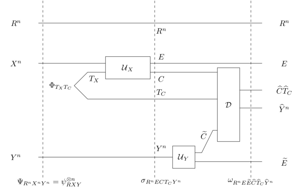
Figure 2: Schematic of the quantum source coding with side information task, the quantum version of the WAK problem.

In Fig. 2, we show a circuit diagram of the most general protocol. Alice’s encoding map ${\mathcal{E}}_{X}:X^{n}T_{X}\to C$ has a Stinespring isometry $\operatorname{\mathcal{U}}_{X}:X^{n}T_{X}\rightarrow CE$. Similarly, Bob’s encoding map ${\mathcal{E}}_{Y}:Y^{n}\to\widetilde{C}$ has a Stinespring isometry $\operatorname{\mathcal{U}}_{Y}:Y^{n}\rightarrow\widetilde{C}\widetilde{E}$. Finally, we denote Charlie’s decoding map as ${\mathcal{D}}:CT_{C}\widetilde{C}\to\widehat{C}\widehat{T}_{C}\widehat{Y}^{n}$; see Fig. 2. The objective is to ensure that the fidelity of the protocol satisfies

$$F_{n} :=\operatorname{Tr}\left(\sigma_{R^{n}ECT_{C}Y^{n}}\omega_{R^{n}E\widehat{C}\widehat{T}_{C}\widehat{Y}^{n}}\right)\to 1\text{ as }n\to\infty,$$ (14)

where

$$\sigma_{R^{n}ECT_{C}Y^{n}}:=\operatorname{\mathcal{U}}_{X}\otimes{\mathrm{id}}_{Y^{n}R^{n}T_{C}}(\psi_{X^{n}Y^{n}R^{n}}\otimes\Phi_{T_{X}T_{C}})$$ (15)

is the overall pure state after Alice’s encoding isometry, and

$$\omega {}_{R^{n}E\widehat{C}\widehat{T}_{C}\widehat{Y}^{n}}$$

$$:={\mathcal{D}}\otimes{\mathrm{id}}_{ER^{n}}\bigl{(}\operatorname{\mathcal{U}}_{X}\otimes{\mathcal{E}}_{Y}\otimes{\mathrm{id}}_{T_{C}R^{n}}(\psi_{X^{n}Y^{n}R^{n}}\otimes\Phi_{T_{X}T_{C}})\bigr{)},$$ (16)

which corresponds to $\operatorname{Tr}_{\widetilde{E}}\omega_{R^{n}E\widetilde{E}\widehat{C}\widehat{T}_{C}\widehat{Y}^{n}}$, with $\omega_{R^{n}E\widetilde{E}\widehat{C}\widehat{T}_{C}\widehat{Y}^{n}}$ the state on the right in Fig. 2. If there are encodings and decodings as above, for which Eq. (14) holds, i.e. the error incurred vanishes in the asymptotic limit, then we say that the corresponding rate pair $(Q_{X},Q_{Y})$ is achievable.

Observe that by definition and by the time sharing principle, the set of achievable rate pairs for a given source is closed, convex and extends to the above right of the $Q_{X}-Q_{Y}$ plane; see Fig. 3. Consequently, the achievable region in the plane is entirely described by its left-lower boundary, the graph of a convex and monotonically non-increasing function.

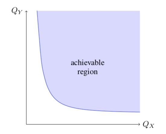
Figure 3: Schematic of the achievable rate region for the assisted source coding task. The achievable rate pairs $(Q_{X},Q_{Y})$ form a closed and convex set extending to the above right.

Theorem 2 (Hsieh/Watanabe [16, Thm. 7])

For a given state $\rho_{XY}$ with purification $\psi_{XYR}$, the rate pair $(Q_{X},Q_{Y})$ is achievable if and only if

$$Q_{Y}\geq\inf_{\operatorname{\mathcal{N}}^{X\to W}\atop{\frac{1}{2}I(W;YR)_{\sigma}\geq Q_{X}}}\frac{1}{2}I(Y;RV)_{\sigma},$$ (17)

where $\operatorname{\mathcal{U}}_{\operatorname{\mathcal{N}}}$ is the Stinespring isometry of $\operatorname{\mathcal{N}}^{X\to W}$ and $\sigma_{WVYR}:=(\operatorname{\mathcal{U}}_{\operatorname{\mathcal{N}}}\otimes{\mathrm{id}}_{YR})\psi_{XYR}$ In other words, the rate pair $(Q_{X},Q_{Y})$ is achievable if and only if

$$Q_{Y}\geq H(Y)-\frac{1}{2}I^{q}_{Y}(2Q_{X}),$$ (18)

where $I^{q}_{Y}(R_{q})$ is the inverse of $R_{q}(I^{q}_{Y})$. ∎

The proof of the achievability part of the theorem is illustrated in Fig. 4. It employs the following two basic protocols as building blocks: the Quantum Reverse Shannon Theorem (QRST) [17, 18], aka state splitting, and Fully quantum Slepian-Wolf (FQSW) [18], aka coherent state merging. For completeness, we provide the full proof in the appendix.

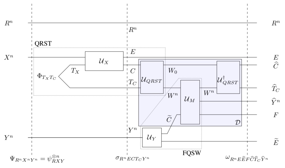
Figure 4: A schematic depiction of the protocol used to show achievability in the proof of Theorem 2. The blue box shows the different actions that compose the decoder ${\mathcal{D}}$. The dotted boxes mark the implementations of the QRST protocol and the FQSW protocol. In particular, $\operatorname{\mathcal{U}}_{QRST}:CT_{C}\to W^{n}W_{0}$ and $\operatorname{\mathcal{U}}_{M}:W^{n}\widetilde{C}\to W^{n}\widehat{Y}^{n}F$ denote the decoding unitary and isometry for QRST and FQSW, respectively.

V Privacy funnel

We can also define a quantum generalization of the so-called privacy funnel function, which is closely related to the information bottleneck function. The concept of privacy funnel was first introduced in [19], where the (classical) privacy funnel function is defined as

$$G(t) =\min_{p(w|x)\atop{I(X;W)\geq t}}I(Y;W),\quad\text{for}\ t\geq 0.$$ (19)

As for the IB function, we can also give a dual function:

$$P(a) =\max_{p(w|x)\atop{I(W;Y)\leq a}}I(X;W),\quad\text{for}\ a\geq 0.$$ (20)

The underlying motivation can be described as follows: Consider a party who is in possession of two correlated sets of data, some public data, $X$, which he is willing to disclose, and some private data, $Y$, which she would like to keep confidential. A second party (usually called an analyst), is granted access to all or parts of the public data, and could exploit the correlations between $X$ and $Y$ to infer information about the private data. The aim of the privacy funnel optimization is to minimize the private information leaked, while providing a sufficient amount of public information for the analyst to use.

In analogy to the information bottleneck, we can give a quantum version of the privacy funnel by considering the following quantity, cf. Eq. (5):

$$G_{q}(t) =\inf_{\operatorname{\mathcal{N}}^{X\to W}\atop{I(YR;W)_{\sigma}\geq t}}I(Y;W)_{\sigma},\quad\text{for}\ t\geq 0.$$ (21)

which again can be equivalently expressed in its dual form

$$P_{q}(a) =\sup_{\operatorname{\mathcal{N}}^{X\to W}\atop{I(Y;W)_{\sigma}\leq a}}I(YR;W)_{\sigma},\quad\text{for}\ a\geq 0.$$ (22)

Proposition 3

The classical and quantum privacy funnel functions, $G(t)$ and $G_{q}(t)$, defined through Eqs. (19) and (21) are convex, i.e. for all $\lambda\in[0,1]$ and $t_{0},t_{1}\geq 0$,

$$G(\lambda t_{0}+(1-\lambda)t_{1}) \leq\lambda G(t_{0})+(1-\lambda)G(t_{1}),$$ (23)

$$G_{q}(\lambda t_{0}+(1-\lambda)t_{1}) \leq\lambda G_{q}(t_{0})+(1-\lambda)G_{q}(t_{1}).$$ (24)

Proof:

The classical case was previously proven in [20]. The proof of the quantum version follows immediately from the same approach as that of Theorem 1. ∎

It would be interesting to find an operational interpretation of $G(t)$ or $G_{q}(t)$. Here, we will not attempt that, but only point out that it probably will not work along similar lines as we have seen for the information bottleneck function, i.e. as rates in an asymptotic i.i.d. setting. Indeed, in [20] it is shown that the classical privacy funnel function is convex and obeys the piecewise linear lower bound

$$G(t)\geq\max\{0,t-H(X|Y)\},$$ (25)

which is 0 up for t between 0 and $H(X|Y)$, and linear with slope 1 for t in the interval from $H(X|Y)$ to $H(X)$. It is also shown that $G(t)$ in general is different from this lower bound, namely even in the neighborhood of $t=0$ it is typically positive, because in [20] it is shown that the derivative at $t=0$ is typically positive. However, this is not the case for the privacy funnel function $G^{(n)}(t)$ of $X^{n}Y^{n}$, as $n\rightarrow\infty$.

Indeed, we claim that

$$G^{(\infty)}(t):=\inf_{n}\frac{1}{n}G^{(n)}(nt)=\max\{0,t-H(X|Y)\}.$$ (26)

Proof:

Note first that also $G^{(\infty)}(t)$ is convex, and that the lower bound from [20] still applies, $G^{(\infty)}(t)\geq\max\{0,t-H(X|Y)\}$. Hence, to show equality, it will be enough to prove that $G^{(\infty)}(H(X|Y))=0$. This follows from privacy amplification by random hashing [21] of $X^{n}$ with the eavesdropper’s information $Y^{n}$: It is possible to extract $W$ as a deterministic function of $X^{n}$, taking values in $\{0,1\}^{nR}$, such that $R$ converges to $H(X|Y)$, and at the same time $I(W;Y^{n})$ goes to $0$. ∎

Since information theoretic interpretations tend to address this i.i.d. limit, it seems unlikely that $G(t)$, rather than $G^{(\infty)}(t)$, can be interpreted in this vein. By analogy, we suspect that $G_{q}(t)$ has the same issues of non-additivity, but leave a thorough discussion of it to another occasion.

VI Numerics and examples

In this section we discuss some examples in order to give an intuition for the information bottleneck and privacy funnel functions and their properties. For better comparison, we choose to normalize the IB function in the following way (as is done in [15]):

$${\overline{R}}_{q}(a) =\inf_{\operatorname{\mathcal{N}}^{X\to W}\atop{\frac{I(Y;W)_{\rho}}{I(Y;X)_{\rho}}\geq a}}\frac{I(X^{\prime};W)_{\tilde{\tau}}}{I(X^{\prime};X)_{\tau}},\quad\text{for}\ a\geq 0.$$ (27)

As before,

$${\tilde{\tau}}_{X^{\prime}W} :=({\rm{id}}_{X^{\prime}}\otimes\operatorname{\mathcal{N}}^{X\to W})\tau_{X^{\prime}X},$$ (28)

where $\tau_{X^{\prime}X}$ is a purification of $\rho_{X}$, and $\sigma_{WY}:=(\operatorname{\mathcal{N}}^{X\to W}\otimes{\rm{id}}_{Y})\rho_{XY}$. This choice of normalization is simply motivated by the data-processing inequality for the mutual information.

\begin{overpic}[trim=170.71652pt 284.52756pt 162.18062pt 284.52756pt,clip,scale={0.8}]{ex3b02234.pdf} \put(-14.0,213.0){${\overline{R}}_{q}(a)$} \put(108.0,0.0){$a$} \end{overpic}

\begin{overpic}[trim=0.0pt 4.26773pt 540.60236pt 310.13486pt,clip,scale={0.8}]{ex3dim3.pdf} \put(-11.0,211.0){${\overline{R}}_{q}(a)$} \put(109.0,0.0){$a$} \end{overpic}

Figure 5: The normalized IB function for the example state $\rho_{XY}^{(3)}$, on the left with $p=0.2$ and on the right with $p=0.4$, each with different allowed dimension for the system $W$. The blue line is $|W|=2$, red is $|W|=3$ and black is $|W|=4$. The red and black line seem to be identical in both cases.

For the numerical examples, we use an improved version of the algorithm described in the supplemental material of [15]. We implemented two main features that are not present in the original code:

• In the code provided along with [15], not only is $|X|=|Y|=2$ fixed, but also $|W|=2$; we removed the latter restriction.

• We adapted the code to also evaluate the privacy funnel function.

Let us first focus on the implications of the first point. A priori the size of the system $W$ could be chosen arbitrarily big to aid the optimization. In the classical case it is known that choosing $|W|=|X|+2$ is always sufficient to reach the optimum [10]. However, in the quantum setting, such a bound is not known and constitutes an important open problem. Now, we can easily give an example where this does in fact play a role. Consider the state

$$\rho_{XY}^{(3)}=p|v\rangle\langle v|+(1-p)|w\rangle\langle w|,$$ (29)

with $|v\rangle=\frac{1}{\sqrt{2}}(|00\rangle+|11\rangle)$ and $|w\rangle=|11\rangle$ (this is also example state $\rho_{XY}^{(3)}$ in [15]).

In Fig. 5 the IB function for the above state is given for $p=0.2$ and $p=0.4$. The blue line corresponds to the example given in [15] with $|W|=2$. One can directly see that lower values can be achieved for $|W|>2$, but it also suggests that nothing can be gained from choosing $|W|>3$ (for this particular example).

Furthermore, this new example suggests that the non-differentiability at $a=0.5$ observed in [15] is rather a result of the $W$ system being too small. Interestingly, for a different example (state $\rho_{XY}^{(2)}$ in [15]) we do not find an advantage up to $|W|=16$ and the non-differentiable point remains. It might however be possible that $|W|$ simply needs to be chosen to be even larger.

Utilizing the second improvement in the algorithm, we can also plot the privacy funnel (PF) function and compare it with the IB function. Again we use a normalized function:

$${\overline{P}}_{q}(a) =\sup_{\operatorname{\mathcal{N}}^{X\to W}\atop{\frac{I(Y;W)_{\rho}}{I(Y;X)_{\rho}}\leq a}}\frac{I(X^{\prime};W)_{\tau}}{I(X^{\prime};X)_{\tau}},\quad\text{for}\ a\geq 0.$$ (30)

An example for $\rho_{XY}^{(3)}$ with $p=0.4$ can be seen in Fig. 6.

Another simple example is that of a pure state $\rho_{XY}=\psi_{XY}$. Here it is clear that the purification $\tau_{X^{\prime}X}$ is equivalent to $\psi_{XY}$ up to an isometry on the $Y$ system. Since this isometry commutes with the channel $\operatorname{\mathcal{N}}$, we immediately obtain $I(Y;W)_{\rho}=I(X^{\prime};W)_{\tau}$ and $I(Y;X)_{\rho}=I(X^{\prime};X)_{\tau}$, and therefore ${\overline{R}}_{q}(a)={\overline{P}}_{q}(a)=a$.

\begin{overpic}[trim=136.5733pt 290.21802pt 85.35826pt 290.21802pt,clip,scale={0.8}]{IBPF.pdf} \put(15.0,213.0){${\overline{R}}_{q}(a)$ and ${\overline{P}}_{q}(a)$} \put(170.0,0.0){$a$} \end{overpic}

Figure 6: The normalized IB and privacy funnel functions for $\rho_{XY}^{(3)}$ with $p=0.4$. The IB function is red, the privacy funnel function is blue. The solid lines use $|W|=3$ and the dashed ones $|W|=2$.

As a final example, we consider the case where $\rho_{XY}$ is a classical state, i.e.

$$\rho_{XY}=\sum_{x,y}p(x,y)|x\rangle\langle x|\otimes|y\rangle\langle y|$$ (31)

where $\{|x\rangle\}$ and $\{|y\rangle\}$ denote orthonormal bases associated with the systems $X$ and $Y$, respectively. In [14] it was shown that for this particular case a classical system $W$ is sufficient for achieving the optimum in the quantum IB function. It follows that the quantum IB function reduces to the classical IB function when the initial state $\rho_{XY}$ is classical. This allows us to verify the numerical algorithm we are using to compute the quantum IB function by the following example: Consider $X$ and $Y$ to be two binary random variables, with $X$ having a uniform distribution, and $Y$ resulting from the action of a binary symmetric channel, with crossover probability $\delta$, on $X$. This example comes with one particular advantage, that is we can give an analytical expression for the classical IB function. In [11] it was shown that in this case the following holds:

$$F(a)=h(h^{-1}(a)\star\delta),$$ (32)

where $F(a)$ is defined in Eq. (3), $h(x)$ is the binary entropy and $\star$ denotes the binary convolution. This is an important example as it plays a crucial role in the theory of classical and quantum information combining [22, 23]. Now, using the reasoning after Eq. (3), one can easily get an expression for the classical IB function to which we apply the same normalization as for the quantum function, denoting the result as ${\overline{R}}(a)$. Plotting values of the classical IB function obtained analytically, and the values of the quantum IB function obtained numerically, results in Fig. 7 and also serves to verify the used numerical algorithm.

The classical example furthermore exhibits an interesting behavior. Namely, we observe that ${\overline{R}}_{q}(1)=\frac{1}{2}$, which turns out to be the same for all classical states $\rho_{XY}$. In [15] it was suggested that this can be understood in terms of quantum teleportation. However, this property should rather be understood as an artifact of the normalization we used when defining ${\overline{R}}_{q}(a)$ and the fact that the system $W$ can be chosen to be classical. For the states defined in Eq. (28), note that $I(X^{\prime};X)_{\tau}=2H(X)_{\tau}$ as $\tau$ is a pure state. On the other hand, we can write $I(X^{\prime};W)_{\tilde{\tau}}=H(X^{\prime})_{\tilde{\tau}}-H(X^{\prime}|W)_{\tilde{\tau}}$ and since the conditional entropy is always positive for classical states (but not necessarily for quantum states), we get for this case $I(X^{\prime};W)_{\tilde{\tau}}\leq H(X^{\prime})_{\tilde{\tau}}=H(X)_{\tau}$. Applying both to Eq. (27) we get that for classical states $\rho_{XY}$ we have ${\overline{R}}_{q}(a)\leq\frac{1}{2}$.

Note, that, with the same reasoning, ${\overline{R}}_{q}(a)\leq\frac{1}{2}$ also holds for quantum states $\rho_{XY}$ when we restrict $W$ to be a classical system (as was previously obtained in [14], by considering the unnormalized function).

\begin{overpic}[trim=123.76965pt 290.21802pt 85.35826pt 290.21802pt,clip,scale={0.75}]{classical.pdf} \put(15.0,206.0){${\overline{R}}_{q}(a)$ and ${\overline{R}}(a)$} \put(170.0,-2.0){$a$} \end{overpic}

Figure 7: The normalized classical and quantum IB function for a classical state defined via a binary symmetric channel with $\delta=0.9$. The classical IB function is in yellow and the quantum IB function in black.

VII Conclusions

We have demonstrated the convexity of the quantum IB function, completing the proof of an operational interpretation for it proposed in [15]. Furthermore we provided a different interpretation coming from source coding with side information at the decoder, via prior work by Hsieh and Watanabe [16]. Along the way we gave an alternative formulation of the quantum IB function that might be useful for its further investigation.

Nevertheless, many open problems remain. These include the question whether entanglement is at all necessary in the source coding task, or if one can remove the requirement of exponentially limited amount of entanglement in the converse.

Some other questions are motivated by the properties we know of the classical IB function. For example, classically it is an easy consequence of Caratheodory’s theorem that the output dimension of the channel that we optimize over can be restricted to $|W|\leq|X|+2$, where $|X|$ is the dimension of the input system [10]. Finding an analogue of this for the quantum case would be extremely useful for the evaluation of the quantum IB function and for its practical application.

Furthermore, considering the variety of applications of the classical IB function it would be interesting to see which of them translate to the quantum setting. Finally, the classical IB function is closely related to entropic bounds on information combining, and our results might help to better understand their quantum generalization [23].

Appendix A Proof of Theorem 2

Here we give the complete proof of Theorem 2; it is essentially the proof found in [16], only that we provide a bit more detail in some places, and that our converse proof is based on a general additivity statement, showing also the additivity of the achievable rate region for a tensor product of two arbitrary sources.

The following two well-known protocols will be employed in the following to construct the achievability part of the proof.

(I) Quantum Reverse Shannon Theorem (QRST), aka state splitting [17, 18]:

Suppose two parties (say, Alice and Bob) are in different locations but share an unlimited amount of entanglement, and let $\operatorname{\mathcal{N}}^{A\to B}$ denote a quantum channel. With respect to an input source $\rho_{A}^{\otimes n}$ of Alice, the output of the channel $\operatorname{\mathcal{N}}^{\otimes n}$ can be simulated at Bob’s end, with asymptotically (in $n$) vanishing error, provided Alice sends qubits at the following rate to Bob:

$$\frac{1}{2}I(B;R)_{\omega},$$ (33)

where $\omega:={(\operatorname{\mathcal{N}}\otimes{\mathrm{id}}_{R})\psi^{\rho}_{AR}}$, with $\psi^{\rho}_{AR}$ being a purification of $\rho_{A}$.

In more detail, this means the following: Let ${\mathcal{U}}_{\operatorname{\mathcal{N}}}^{A\to BE}$ denote the Stinespring isometry of the quantum channel, with $E$ denoting the environment. Then, the initial state of the protocol is $\Psi_{A^{n}R^{n}}:=\left(\psi^{\rho}_{AR}\right)^{\otimes n}\otimes\Phi_{T_{A}T_{B}}$, where by $\Phi_{T_{A}T_{B}}$ we denote the entangled state initially shared between Alice and Bob. After execution of the protocol, for $n$ large enough, the purifying reference system $R^{n}$ remains unchanged, while with asymptotically vanishing error, Alice receives the environment system $E^{n}$, while Bob receives the system $B^{n}$ of the state $|\psi\rangle_{B^{n}E^{n}R^{n}}:=(|\psi\rangle_{BER})^{\otimes n}$, with $|\psi\rangle_{BER}={\mathcal{U}}_{\operatorname{\mathcal{N}}}^{A\to BE}|\psi^{\rho}\rangle_{AR}$.

(II) Fully Quantum Slepian-Wolf (FQSW), aka coherent state merging [18]:

Suppose two distant parties (say Bob and Charlie) share the state $\sigma_{B^{n}C^{n}}\equiv\sigma_{BC}^{\otimes n}$. Consider its purification $\varphi_{B^{n}C^{n}R^{n}}\equiv\varphi_{BCR}^{\otimes n}$, with $\varphi_{BCR}$ being a purification of $\sigma_{BC}$. Then by implementing the FQSW protocol, Bob can transmit the state of his system $B^{n}$ (and also the entanglement initially shared between $B^{n}$ and $R^{n}$), with asymptotically vanishing error, to Charlie, by sending qubits at a rate

$$\frac{1}{2}I(B;R)_{\varphi},$$

to him.

Proof Theorem 2.  (Achievability): This part of the proof follows directly by applying the previously described QRST and FQSW protocols (see also Fig. 4). Let $\rho_{X}:=\operatorname{Tr}_{YR}\psi_{XYR}$ and $\psi_{X^{n}Y^{n}R^{n}}:=\psi_{XYR}^{\otimes n}$. For $n$ large enough, by using the shared entangled state $\Phi_{T_{X}T_{C}}$ and employing the QRST protocol, Alice and Charlie can simulate the output of $n$ independent uses of an encoding map (i.e. a quantum channel) $\operatorname{\mathcal{N}}^{X\to W}$, corresponding to an input $\rho_{X}^{\otimes n}$, with asymptotically vanishing error, provided Alice sends qubits to Charlie, via a system $C$ at a rate $\frac{1}{2}I(W;RY)_{\omega}$, where $\omega:=(\operatorname{\mathcal{N}}^{X\to W}\otimes{\rm{id}}_{YR})\psi_{XYR}$. Once Charlie receives the system $C$ from Alice, the composite system in his possession is $\overline{C}:=CT_{C}$.

Next, by implementing the FQSW protocol on the tripartite state $\sigma_{R^{n}ECT_{C}Y^{n}}$, with $R^{n}E$, $CT_{C}$ and $Y^{n}$ being the three systems in the tripartition, Bob can transmit his system $Y^{n}$ to Charlie, with asymptotically vanishing error, by sending qubits to him at a rate $Q_{Y}=\frac{1}{2}I(Y;RE)_{\sigma}=\frac{1}{2}I(Y;RV)_{\sigma}$, where the equality follows since the system $E$ resulting from applying the FQSW protocol is identical to the purifying system $V$ of the simulated channel $\operatorname{\mathcal{N}}^{X\to W}$.

Minimizing over all possible encoding maps of Alice, yields the expression on the right hand side of (17), thus establishing it as an achievable rate of the specified task.

(Converse/Optimality): Consider the most general protocol under which Alice and Bob, by performing local operations and by sending qubits at a rate $Q_{X}$ and $Q_{Y}$, respectively, to Charlie, can transmit the states $C$, $T_{C}$ and $Y^{n}$ to him.

We assume that there are noiseless quantum channels between Alice and Charlie, and Bob and Charlie. Alice’s most general operation may be decomposed into two steps: (i) she locally generates a maximally entangled state $\Phi_{T_{X}T_{C}}$ and sends $T_{C}$ to Charlie; at the end of this step she has the systems $X^{n}T_{X}$, while Charlie has the system $T_{C}$; (ii) she then applies her encoding map, a CPTP map ${\mathcal{E}}^{X^{n}T_{X}\to C}$, whose Stinespring isometry we denote as $\operatorname{\mathcal{U}}_{{\mathcal{E}}}^{X^{n}T_{X}\to CE}$. Let

$$\sigma_{R^{n}ECT_{C}Y^{n}}:=\left(\operatorname{\mathcal{U}}_{{\mathcal{E}}}^{X^{n}T_{X}\to CE}\!\!\otimes{\mathrm{id}}_{Y^{n}R^{n}T_{C}}\!\right)\!(\psi_{X^{n}Y^{n}R^{n}}\!\otimes\!\Phi_{T_{X}T_{C}}).$$ (34)

In the above, $X^{n}=X_{1}X_{2}\ldots X_{n}$, $Y^{n}=Y_{1}Y_{2}\ldots Y_{n}$ and $R^{n}=R_{1}R_{2}\ldots R_{n}$.

The rate at which Alice transmits qubits to Charlie is $Q_{X}=\frac{1}{n}{\log|C|}$. Hence,

$$nQ_{X} \geq H(C)_{\sigma},$$

$$\geq\frac{1}{2}I(C;Y^{n}R^{n}T_{C})_{\sigma},$$

$$\geq\frac{1}{2}I(C;Y^{n}R^{n}|T_{C})_{\sigma},$$

$$=\frac{1}{2}I(CT_{C};Y^{n}R^{n})_{\sigma},$$

$$\equiv\frac{1}{2}I(\overline{C};Y^{n}R^{n})_{\sigma},$$ (35)

where $\overline{C}=CT_{C}$; observe that the above reasoning allows us to integrate the steps (i) and (ii) of Alice’s operation into a single CPTP map $\overline{{\mathcal{E}}}:X^{n}\longrightarrow\overline{C}$, acting as $\overline{{\mathcal{E}}}(\rho)=({\mathcal{E}}\otimes{\mathrm{id}}_{T_{C}})(\rho_{X^{n}Y^{n}}\otimes\Phi_{T_{X}T_{C}})$, where $\rho_{X^{n}Y^{n}}=\operatorname{Tr}_{R^{n}}\psi_{X^{n}Y^{n}R^{n}}$. Now, the first inequality follows because $H(C)\leq\log|C|$, the second inequality follows from the fact that for a pure state of a tripartite system $ABE$,

$$H(A)=\frac{1}{2}I(A;B)+\frac{1}{2}I(A;E)\geq\frac{1}{2}I(A;B),$$ (36)

the third inequality holds because of the chain rule

$$I(A;BC) =I(A;B)+I(A;C|B),$$ (37)

where for any tripartite state $\rho_{ABC}$, $I(A;C|B):=H(\rho_{AB})+H(\rho_{BC})-H(\rho_{B})-H(\rho_{ABC})$ denotes the conditional mutual information. The equality follows because $T_{C}$ is uncorrelated with $Y^{n}R^{n}$.

Suppose it suffices for Bob to transmit qubits at a rate $Q_{Y}=\frac{1}{n}{\log|{\widetilde{C}}|}$ to Charlie. Let $\operatorname{\mathcal{U}}^{Y^{n}\to{\widetilde{C}}\widetilde{E}}$ be a unitary that Bob performs, and

$$\omega_{R^{n}E{\widetilde{C}}\widetilde{E}}=({\mathrm{id}}_{R^{n}E}\otimes\operatorname{\mathcal{U}}^{Y^{n}\to{\widetilde{C}}\widetilde{E}})\sigma_{R^{n}EY^{n}}.$$

Then $\widetilde{E}$ must be decoupled from $R^{n}V$ in the asymptotic limit. This is because the fidelity criterion in Eq. (14) ensures that the final state $\omega_{R^{n}E\widehat{C}\widehat{T}_{C}\widehat{Y}^{n}}$ is close to a pure state. Indeed, the fidelity bound $F\left(\sigma_{R^{n}ECT_{C}Y^{n}},\omega_{R^{n}E\widehat{C}\widehat{T}_{C}\widehat{Y}^{n}}\right)^{2}\geq 1-\epsilon$ implies, by Uhlmann’s theorem, that there exists a state $\tau_{\widetilde{E}}$ such that

$$F\left(\sigma_{R^{n}ECT_{C}Y^{n}}\otimes\tau_{\widetilde{E}},\omega_{R^{n}E\widehat{C}\widehat{T}_{C}\widehat{Y}^{n}\widetilde{E}}\right)^{2}\geq 1-\epsilon,$$

which implies in particular that

$$F\left(\sigma_{R^{n}E}\otimes\tau_{\widetilde{E}},\omega_{R^{n}E\widetilde{E}}\right)^{2}\geq 1-\epsilon.$$

Using the well-known relations between fidelity and trace distance, this yields

$$\frac{1}{2}\left\|\sigma_{R^{n}E}\otimes\tau_{\widetilde{E}}-\omega_{R^{n}E\widetilde{E}}\right\|_{1}\leq\sqrt{\epsilon}.$$

Hence, by the Alicki-Fannes inequality regarding the continuity of the quantum conditional entropy [24, 25], for any $\delta>0$ and for large enough $n$,

$$\frac{1}{2}I(\widetilde{E};R^{n}E)_{\omega} \leq{n{\delta}}.$$ (38)

Namely,

$$\begin{split}I(\widetilde{E};R^{n}E)_{\omega}&=I(\widetilde{E};R^{n}E)_{\omega}-I(\widetilde{E};R^{n}E)_{\sigma\otimes\tau}\\ &\leq\bigl{|}S(\omega_{\widetilde{E}})-S(\tau_{\widetilde{E}})\bigr{|}\\ &\phantom{===}+\bigl{|}S(\widetilde{E}|R^{n}E)_{\omega}-S(\widetilde{E}|R^{n}E)_{\sigma\otimes\tau}\bigr{|}\\ &\leq 3\sqrt{\epsilon}\log|\widetilde{E}|+2(1+\sqrt{\epsilon})h\left(\frac{\sqrt{\epsilon}}{1+\sqrt{\epsilon}}\right),\end{split}$$

where $h(x)=-x\log x-(1-x)\log(1-x)$ is the binary entropy. To conclude this part of the argument, notice that w.l.o.g. $|\widetilde{E}|\leq|Y|^{n}|\widetilde{C}|\leq(|Y|2^{Q_{Y}})^{n}$, and so Eq. (38) holds with $\delta=(3\log|Y|+3Q_{Y})\sqrt{\epsilon}+\frac{4}{n}$, which can be made arbitrarily small for sufficiently large $n$.

Since $Q_{Y}=\frac{1}{n}{\log|{\widetilde{C}}|}$, we have

$$nQ_{Y} \geq H({\widetilde{C}})_{\omega},$$

$$\geq\frac{1}{2}I({\widetilde{C}};R^{n}E\widetilde{E})_{\omega},$$

$$\geq\frac{1}{2}I({\widetilde{C}};R^{n}E|\widetilde{E})_{\omega},$$

$$=\frac{1}{2}I({\widetilde{C}}\widetilde{E};R^{n}E)_{\omega}-\frac{1}{2}I(\widetilde{E};R^{n}E)_{\omega}$$

$$\geq\frac{1}{2}I({Y^{n}};R^{n}E)_{\sigma}-{n{\delta}},$$ (39)

where the first inequality follows because $H({\widetilde{C}})\leq\log|{\widetilde{C}}|$, the second inequality follows again from Eq. (36), the third inequality and the equality follow from the chain rule (37) and the last inequality follows from the fact that the mutual information is invariant under unitaries (note that the states of ${\widetilde{C}}\widetilde{E}$ and $Y^{n}$ are related by a unitary) and (38).

The final step is now to express the bounds (35) and (A) on the rates $Q_{X}$ and $Q_{Y}$ by single-letter expressions. To this end we define the following set for the pure state $\psi\equiv\psi_{XYR}$:

$$\begin{split}{\mathcal{T}}(\psi)&:=\bigl{\{}(Q_{X},Q_{Y}):\exists\,\operatorname{\mathcal{U}}^{X\to WV}\,\text{isometry s.t. }\bigr{.}\\ &\phantom{======}2Q_{X}\geq I(W;YR)_{\sigma},\,2Q_{Y}\geq I(Y;RV)_{\sigma},\\ &\phantom{======}\bigl{.}\sigma_{WVYR}:=(\operatorname{\mathcal{U}}^{X\to WV}\otimes{\mathrm{id}}_{YR})\psi_{XYR}\bigr{\}}.\end{split}$$ (40)

We show below that the set ${\mathcal{T}}(\psi)$ satisfies an additivity property: For any two states ${\psi^{(i)}}_{X_{i}Y_{i}R_{i}}$,

$${\mathcal{T}}(\psi^{(1)}\otimes\psi^{(2)})={\mathcal{T}}(\psi^{(1)})+{\mathcal{T}}(\psi^{(2)}),$$ (41)

where the $+$ on the r.h.s. refers to the Minkowski sum (i.e. element-wise sum) of two sets. Suppose that $(Q_{X},Q_{Y})\in{\mathcal{T}}(\psi^{(1)}\otimes\psi^{(2)})$, where $\psi^{(1)}$ (resp. $\psi^{(2)}$) is a pure state of a tripartite system $X_{1}Y_{1}R_{1}$ (resp. $X_{2}Y_{2}R_{2}$). Alice possesses the systems $X_{1}$ and $X_{2}$, while Bob possesses $Y_{1}$ and $Y_{2}$; here $R_{1}$ and $R_{2}$ denote inaccessible, purifying reference systems. The final composite pure state, resulting from the action of a Stinespring isometry $\operatorname{\mathcal{U}}^{X_{1}X_{2}\to WV}$, is then given by

$$\widetilde{\sigma}_{WVY_{1}Y_{2}R_{1}R_{2}}:=\left(\operatorname{\mathcal{U}}^{X_{1}X_{2}\to WV}\otimes{\mathrm{id}}_{Y_{1}Y_{2}R_{1}R_{2}}\right)(\psi^{(1)}\otimes\psi^{(2)}).$$ (42)

The $\supseteq$ direction follows directly from the fact that $(i)$ the set of all isometries $\operatorname{\mathcal{U}}^{X_{1}X_{2}\to WV}$ clearly also includes all those of the form $\operatorname{\mathcal{U}}^{X_{1}\to W_{1}V_{1}}\otimes\operatorname{\mathcal{U}}^{X_{2}\to W_{2}V_{2}}$, with $\operatorname{\mathcal{U}}^{X_{1}\to W_{1}V_{1}}$ and $\operatorname{\mathcal{U}}^{X_{2}\to W_{2}V_{2}}$ being isometries arising in the definitions of the sets ${\mathcal{T}}(\psi^{(1)})$ and ${\mathcal{T}}(\psi^{(2)})$, and $(ii)$ from the additivity of the mutual information. We will therefore concentrate on the $\subseteq$ direction.

By assumption, and using the chain rule Eq. (37), we obtain

$$2Q_{X_{1}X_{2}} \geq I(W;Y_{1}Y_{2}R_{1}R_{2})_{\widetilde{\sigma}},$$

$$=I(W;Y_{1}R_{1}|Y_{2}R_{2})_{\widetilde{\sigma}}+I(W;Y_{2}R_{2})_{\widetilde{\sigma}}$$

$$=I(Y_{1}R_{1};WY_{2}R_{2})_{\widetilde{\sigma}}+I(W;Y_{2}R_{2})_{\widetilde{\sigma}}$$

$$=:I(Y_{1}R_{1};W_{1})_{\widetilde{\sigma}}+I(Y_{2}R_{2};W_{2})_{\widetilde{\sigma}},$$ (43)

with $W_{1}:=WY_{2}R_{2}$ and $W_{2}:=W$.

Similarly, by using the chain rule (37) twice, the fact that the states of the systems $Y_{1}$ and $Y_{2}$ are uncorrelated (and hence $I(Y_{1};Y_{2})_{\sigma}=0$) and the data-processing inequality (with respect to partial trace) we obtain

$$2Q_{Y_{1}Y_{2}} \geq I(Y_{1}Y_{2};R_{1}R_{2}V)_{\widetilde{\sigma}},$$

$$=I(Y_{1};R_{1}R_{2}V)_{\widetilde{\sigma}}+I(Y_{2};R_{1}R_{2}V|Y_{1})_{\widetilde{\sigma}}$$

$$=I(Y_{1};R_{1}R_{2}V)_{\widetilde{\sigma}}+I(Y_{2};R_{1}R_{2}VY_{1})_{\widetilde{\sigma}}-I(Y_{1};Y_{2})_{\sigma}$$

$$\geq I(Y_{1};R_{1}V)_{\widetilde{\sigma}}+I(Y_{2};R_{1}R_{2}VY_{1})_{\widetilde{\sigma}}$$

$$=:I(Y_{1};R_{1}V_{1})_{\widetilde{\sigma}}+I(Y_{2};R_{2}V_{2})_{\widetilde{\sigma}},$$ (44)

with $V_{1}:=V$ and $V_{2}:=VR_{1}Y_{1}$.

The pure state $\widetilde{\sigma}$ of Eq. (42) of the composite system $WVY_{1}Y_{2}R_{1}R_{2}$ results from the action of the isometry $\operatorname{\mathcal{U}}^{X_{1}X_{2}\to WV}$ on $\psi^{(1)}\otimes\psi^{(2)}$. However, by the above definitions of the systems $W_{1}$, $W_{2}$, $V_{1}$ and $V_{2}$, it follows that one can construct two isometries $\mathcal{U}^{(i)}:X_{i}\rightarrow W_{i}V_{i}$, for $i=1,2$, which when acting solely on the pure state $\psi^{(1)}$ and $\psi^{(2)}$ respectively, yields pure states of this same composite system $WVY_{1}Y_{2}R_{1}R_{2}$. Let these resulting pure states be denoted as $\sigma^{(1)}$ and $\sigma^{(2)}$ respectively:

$$\sigma^{(1)}\equiv\sigma^{(1)}_{W_{1}V_{1}Y_{1}R_{1}} =(\operatorname{\mathcal{U}}^{(1)}\otimes{\mathrm{id}}_{Y_{1}R_{1}})\psi_{X_{1}Y_{1}R_{1}},$$

$$\sigma^{(2)}\equiv\sigma^{(2)}_{W_{2}V_{2}Y_{2}R_{2}} =(\operatorname{\mathcal{U}}^{(2)}\otimes{\mathrm{id}}_{Y_{2}R_{2}})\psi_{X_{2}Y_{2}R_{2}}.$$

Then the bounds (43) and (44) can be rewritten as

$$2Q_{X_{1}X_{2}} \geq I(Y_{1}R_{1};W_{1})_{\sigma^{(1)}}+I(Y_{2}R_{2};W_{2})_{\sigma^{(2)}},$$

$$2Q_{Y_{1}Y_{2}} \geq I(Y_{1};R_{1}V_{1})_{\sigma^{(1)}}+I(Y_{2};R_{2}V_{2})_{\sigma^{(2)}}.$$

However, by definition of the isometries $\operatorname{\mathcal{U}}^{(i)}$ for $i=1,2$, it follows that $I(Y_{i}R_{i};W_{i})_{\sigma^{(i)}}$ and $I(Y_{i};R_{i}V_{i})_{\sigma^{(i)}}$ are respectively valid lower bounds on $2Q_{X_{i}}$ and $2Q_{Y_{i}}$ for pairs $(Q_{X_{i}},Q_{Y_{i}})$ occurring in the sets ${\mathcal{T}}(\psi^{(i)})$.

Hence, we have

$${\mathcal{T}}(\psi^{(1)}\otimes\psi^{(2)})\subseteq{\mathcal{T}}(\psi^{(1)})+{\mathcal{T}}(\psi^{(2)}),$$

and we conclude the additivity property Eq. (41). As an immediate implication, we get by induction, choosing $\psi^{(1)}=\psi$ and $\psi^{(2)}=\psi^{\otimes(n-i)}$ for $i\in\{1,\dots,n-1\}$, that

$${\mathcal{T}}(\psi^{\otimes n})=n{\mathcal{T}}(\psi).$$ (45)

It follows, returning to the bounds (35) and (A), that there is an isometry ${\mathcal{U}}:X\longrightarrow VW$ such that

$$Q_{X} \geq\frac{1}{2}I(W;YR)_{\sigma},$$ (46)

$$Q_{Y} \geq\frac{1}{2}I(Y;RV)_{\sigma}-{{\delta}},$$ (47)

where $\sigma_{WVYR}$ is as in the statement of the theorem. Since $\delta$ becomes arbitrarily small for sufficiently large $n$, we obtain the desired bounds. $\blacksquare$

Remark 4

In the above proof we have used Eq. (41) only to show the single-letterization of the rate region in Theorem 2. Since the result is that ${\mathcal{T}}(\psi)$ is that rate region, the additivity relation (41) shows that the rate region of a product of two independent sources is the Minkowski sum of the individual rate regions.

References

• [1] N. Tishby, F. C. Pereira, and W. Bialek, “The information bottleneck method,” 2000, arXiv:physics/0004057.
• [2] C. E. Shannon, “Coding theorems for a discrete source with a fidelity criterion,” IRE Nat. Conv. Records, vol. 7, pp. 142–163, March 1959.
• [3] T. Berger, Rate distortion theory: A mathematical basis for data compression. Prentice-Hall, 1971.
• [4] T. M. Cover and J. A. Thomas, Elements of Information Theory. John Wiley & Sons, 2012.
• [5] N. Tishby and N. Zaslavsky, “Deep learning and the information bottleneck principle,” in Proc. IEEE Inf. Theory Workshop (ITW), 2015.
• [6] R. Shwartz-Ziv and N. Tishby, “Opening the black box of deep neural networks via information,” 2017, arXiv[cs.IT]:1703.00810.
• [7] W. H. Hsu, L. S. Kennedy, and S.-F. Chang, “Video search reranking via information bottleneck principle,” in Proc. 14th ACM Int’l Conf. Multimedia.ACM, 2006, pp. 35–44.
• [8] N. Slonim and N. Tishby, “Document clustering using word clusters via the information bottleneck method,” in Proc. 23rd Annual Int’l ACM SIGIR Conf. Res. Dev. Information Retrieval, 2000, pp. 208–215.
• [9] M. Stark, A. Shah, and G. Bauch, “Polar code construction using the information bottleneck method,” in Proc. IEEE Wireless Comm. Netw. Conf. Workshops (WCNCW), April 2018, pp. 7–12.
• [10] R. Gilad-Bachrach, A. Navot, and N. Tishby, “An information theoretic tradeoff between complexity and accuracy,” in Proc. Conf. Learning Theory and Kernel Machines, B. Schölkopf and M. K. Warmuth, Eds. LNAI, vol. 2777, Springer Verlag Berlin Heidelberg, 2003, pp. 595–609.
• [11] H. S. Witsenhausen and A. D. Wyner, “A conditional entropy bound for a pair of discrete random variables,” IEEE Trans. Inf. Theory, vol. 21, no. 5, pp. 493–501, 1975.
• [12] A. D. Wyner, “On source coding with side information at the decoder,” IEEE Trans. Inf. Theory, vol. 21, no. 3, pp. 294–300, May 1975.
• [13] R. Ahlswede and J. Körner, “Source coding with side information and a converse for degraded broadcast channels,” IEEE Trans. Inf. Theory, vol. 21, no. 6, pp. 629–637, November 1975.
• [14] A. L. Grimsmo and S. Still, “Quantum predictive filtering,” Phys. Rev. A, vol. 94, 012338, Jul 2016.
• [15] S. Salek, D. Cadamuro, P. Kammerlander, and K. Wiesner, “Quantum rate-distortion coding of relevant information,” 2017, arXiv[quant-ph]:1704.02903.
• [16] M.-H. Hsieh and S. Watanabe, “Channel Simulation and Coded Source Compression,” IEEE Trans. Inf. Theory, vol. 62, no. 11, pp. 6609–6619, 2016.
• [17] I. Devetak, “Triangle of dualities between quantum communication protocols,” Phys. Rev. Lett., vol. 97, 140503, 2006.
• [18] A. Abeyesinghe, I. Devetak, P. Hayden, and A. Winter, “The mother of all protocols: Restructuring quantum information’s family tree,” Proc. Roy. Soc. London A, vol. 465, pp. 2537–2563, June 2009.
• [19] A. Makhdoumi, S. Salamatian, N. Fawaz, and M. Médard, “From the information bottleneck to the privacy funnel,” in Proc. IEEE Inf. Theory Workshop (ITW), 2014, pp. 501–505.
• [20] F. P. Calmon, A. Makhdoumi, M. Médard, M. Varia, M. Christiansen, and K. R. Duffy, “Principal inertia components and applications,” IEEE Trans. Inf. Theory, vol. 63, no. 8, pp. 5011–5038, 2017.
• [21] C. H. Bennett, G. Brassard, C. Crépeau and U. M. Maurer, “Generalized privacy amplification,” IEEE Trans. Inf. Theory, vol. 41, no. 6, pp. 1915–1923, 1995.
• [22] A. D. Wyner and J. Ziv, “A theorem on the entropy of certain binary sequences and applications–I,” IEEE Trans. Inf. Theory, vol. 19, no. 6, pp. 769–772, 1973.
• [23] C. Hirche and D. Reeb, “Bounds on information combining with quantum side information,” IEEE Trans. Inf. Theory, vol. 64, no. 7, pp. 4739–4757, 2018.
• [24] R. Alicki and M. Fannes, “Continuity of quantum conditional information”, J. Phys. A: Math. Gen., vol. 37, no. 5, pp. L55–L57, 2004.
• [25] A. Winter, “Tight Uniform Continuity Bounds for Quantum Entropies: Conditional Entropy, Relative Entropy Distance and Energy Constraints”, Commun. Math. Phys., vol. 347, no. 1, pp. 291–313, 2016.