A necessary and sufficient condition for the stability of linear Hamiltonian systems with periodic coefficients

Abstract

Linear Hamiltonian systems with time-dependent coefficients are of importance to nonlinear Hamiltonian systems, accelerator physics, plasma physics, and quantum physics. It is shown that the solution map of a linear Hamiltonian system with time-dependent coefficients can be parameterized by an envelope matrix $w(t)$, which has a clear physical meaning and satisfies a nonlinear envelope matrix equation. It is proved that a linear Hamiltonian system with periodic coefficients is stable iff the envelope matrix equation admits a solution with periodic $\sqrt{w^{\dagger}w}$ and a suitable initial condition. The mathematical devices utilized in this theoretical development with significant physical implications are time-dependent canonical transformations, normal forms for stable symplectic matrices, and horizontal polar decomposition of symplectic matrices. These tools systematically decompose the dynamics of linear Hamiltonian systems with time-dependent coefficients, and are expected to be effective in other studies as well, such as those on quantum algorithms for classical Hamiltonian systems.

1 Introduction and main results

We consider the following $2n$-dimensional linear Hamiltonian system with periodic time-dependent coefficients,

$$\dot{z} =J\nabla H\thinspace,$$ (1)

$$J =\left(\begin{array}[]{cc}0&I_{n}\\ -I_{n}&0\end{array}\right)\,,$$ (4)

$$H =\frac{1}{2}z^{\dagger}Az\,,\,\,\,A=\left(\begin{array}[]{cc}\kappa\left(t\right)&R\left(t\right)\\ R\left(t\right)^{\dagger}&m^{-1}\left(t\right)\end{array}\right)\,.$$ (7)

Here, $z=\left(x_{1},...,x_{n,}\,p_{1},...,p_{n}\right)^{\dagger}$ are the phase space coordinates, $J$ is the $2n\times 2n$ standard symplectic matrix, and $\kappa(t),$ $R\left(t\right),$ and $m^{-1}\left(t\right)$ are periodic time-dependent $n\times n$ matrices with periodicity $T$. The matrices $\kappa(t)$ and $m^{-1}\left(t\right)$ are symmetric, and $m(t)$ is also invertible. Supper script “$\dagger$” denotes matrix transpose.

We are interested in the stability of the dynamics of system (1) at $t\rightarrow\infty$. The system is called stable if $\lim_{t\rightarrow\infty}z(t)$ is bounded for all initial conditions $z_{0}=z(t=0).$ The solution of system (1) can be specified by a solution map,

$$z(t)=M(t)z_{0}\,.$$ (8)

A matrix $M$ is called stable if $\lim_{l\rightarrow\infty}M^{l}$ is bounded, which is equivalent to the condition that $M$ is diagonalizable with all eigenvalues on the unit circle of the complex plane. In terms of the one-period solution map $M(T)$, system (1) is stable iff $M(T)$ is stable.

The main results of the paper are summarized in the following two theorems.

Theorem 1.

The solution map of linear Hamiltonian system (1) can be written as

$$M(t)=S^{-1}P^{-1}S_{0},$$ (9)

where

$$S \equiv\left(\begin{array}[]{cc}w^{\dagger-1}&0\\ (wR-\dot{w})m&w\end{array}\right)\,,$$ (12)

$$S_{0} \equiv S(t=0)\,,$$ (13)

$w(t)$ is a time-dependent $n\times n$ matrix satisfying the envelope equation

$$\frac{d}{dt}\left(\frac{dw}{dt}m-wRm\right) +\frac{dw}{dt}mR^{\dagger}+w\left(\kappa-RmR^{\dagger}\right)-\left(w^{\dagger}wmw^{\dagger}\right)^{-1}=0\,,$$ (14)

and $P(t)\in Sp(2n,\mathbb{R})\cap O(2n,\mathbb{R})$ is determined by

$$\dot{P}=P\left(\begin{array}[]{cc}0&-\mu\\ \mu&0\end{array}\right)\,,$$ (17)

$$\mu=\left(wmw^{\dagger}\right)^{-1}\,.$$ (18)

Theorem 2.

The linear Hamiltonian system (1) is stable iff the envelope equation (14) admits a solution $w(t)$ such that $S_{0}$ is symplectic and $|w|\equiv\sqrt{w^{\dagger}w}$ is periodic with periodicity $T.$

The solution map given in Theorem 1 is constructed using a time-dependent canonical transformation method. Note that Theorem 1 is valid regardless whether the coefficients of the Hamiltonian are periodic or not. Techniques of normal forms for stable symplectic matrices and horizontal polar decomposition for symplectic matrices are developed to prove Theorem 2. The results and techniques leading to Theorem 1 have been reported previously in the context of charged particle dynamics in a general focusing lattice (Qin and Davidson, 2009a, b; Qin et al., 2009, 2010; Chung et al., 2010; Qin and Davidson, 2011, 2013; Qin et al., 2013; Chung et al., 2013; Qin et al., 2014, 2015; Chung et al., 2015, 2016a, 2016b; Chung and Qin, 2018). These contents are included here for easy reference and self-consistency.

In Sec. 2, we will discuss the significance of the main results and their applications in physics. Section 3 describes the method of time-dependent canonical transformation, and Sec. 4 is devoted to the construction of the solution map as given in Theorem 1. The normal forms of stable symplectic matrices are presented in Sec. 5, and the horizontal polar decomposition of symplectic matrices is introduced in Sec. 6. The proof of Theorem 2 is completed in Sec. 7.

2 Significance and applications

Linear Hamiltonian systems with time-dependent coefficients (1) has many important applications in physics and mathematics. In accelerator physics, it describes charged particle dynamics in a periodic focusing lattice (Davidson and Qin, 2001). The dynamic properties, especially the stability properties, of the system to a large degree dictate the designs of beam transport systems and storage rings for modern accelerators. In the canonical quantization approach for quantum field theory, Schrödinger’s equation in the interaction picture, which is the starting point of Dyson’s expansion, S-matrix and Feynman diagrams, assumes the form of a linear Hamiltonian system with time-dependent coefficients. For nonlinear Hamiltonian dynamics, nonlinear periodic orbit is an important topic. The stability of nonlinear periodic orbits are described by linear Hamiltonian systems with periodic coefficients.

To illustrate the significance of the main results of this paper, we look at the implications of Theorems 1 and 2 for the special case of one degree of freedom with $m=1$, for which Hamilton’s equation (1) reduces to the harmonic oscillator equation with a periodic spring constant,

$$\ddot{x}+\kappa(t)x=0\,.$$ (19)

According to Theorem 1, the solution of Eq. (19) is

$$\left(\begin{array}[]{c}x\\ \dot{x}\end{array}\right) =M(t)\left(\begin{array}[]{c}x\\ \dot{x}\end{array}\right)_{0}\,.$$ (24)

$$M\left(t\right) =S^{-1}\left(\begin{array}[]{cc}\cos\phi&\sin\phi\\ -\sin\phi&\cos\phi\end{array}\right)S_{0}\,,$$ (27)

$$S =\left(\begin{array}[]{cc}w^{-1}&0\\ -\dot{w}&w\end{array}\right)\,,$$ (30)

$$\phi\left(t\right) =\int_{0}^{t}\dfrac{dt}{w^{2}}\,,$$ (31)

where the scalar envelope function $w\left(t\right)$ satisfies the nonlinear envelope equation

$$\ddot{w}+\kappa\left(t\right)w=w^{-3}\,.$$ (32)

This solution for Eq. (19) and the scalar envelope equation (32) were discovered by Courant and Snyder (Courant and Snyder, 1958) in the context of charged particle dynamics in one-dimensional periodic focusing lattices. The solution map given by Courant and Snyder (Courant and Snyder, 1958) is

$$M\left(t\right)=\left(\begin{array}[]{cc}\sqrt{\dfrac{\beta}{\beta_{0}}}\left[\cos\phi+\alpha_{0}\sin\phi\right]&\sqrt{\beta\beta_{0}}\sin\phi\\ -\dfrac{1+\alpha\alpha_{0}}{\sqrt{\beta\beta_{0}}}\sin\phi+\dfrac{\alpha_{0}-\alpha}{\sqrt{\beta\beta_{0}}}\cos\phi&\sqrt{\dfrac{\beta_{0}}{\beta}}\left[\cos\phi-\alpha\sin\phi\right]\end{array}\right)\,,$$ (33)

where the $\alpha$ and $\beta$ are time-dependent functions defined as $\alpha\left(t\right)=-w\dot{w}$ and $\beta\left(t\right)=w^{2}\left(t\right),$ and $\alpha_{0}$ and $\beta_{0}$ are initial conditions at $t=0.$ It equals the $M$ in the three-way splitting form in Eq. (27).

The scalar $w(t)$ is called the envelope because it encapsulates the slow dynamics of the envelope for the fast oscillation, when the variation time-scale of $\kappa(t)$ is slow compared with the period determined by $\kappa(t)$, i.e,

$$\left|\frac{d\kappa}{\kappa dt}\right|\ll\sqrt{\left|k\right|}\,.$$ (34)

Since the solution map gives the solution of the dynamics in terms of $w$, invariants of the dynamics can also be constructed. For example, the Courant-Synder invariant (Courant and Snyder, 1958) is

$$I_{CS}=\dfrac{x^{2}}{w^{2}}+\left(w\dot{x}-\dot{w}x\right)^{2}\,,$$ (35)

which was re-discovered by Lewis in classical and quantum settings (Lewis, 1968; Lewis and Riesenfeld, 1969) . The envelope equation is also known as the Ermakov-Milne-Pinney equation (Ermakov, 1880; Milne, 1930; Pinney, 1950), which has been utilized to study 1D time-dependent quantum systems (Lewis, 1968; Lewis and Riesenfeld, 1969; Morales, 1988; Monteoliva et al., 1994) and associated non-adiabatic Berry phases (Berry, 1985). Given that harmonic oscillator is the most important physics problem, it comes as no surprise that Eq. (19) had been independently examined many times from the same or different angles over the history (Qin and Davidson, 2006).

When specialized to the system with one degree of freedom (19), Theorem 2 asserts that the dynamics is stable iff the envelope equation (32) admits a periodic solution with periodicity $T$. The theorem emphasizes again the crucial role of the envelope $w$ in determining the dynamic properties of the system. The sufficiency is straightforward to establish. If $w(t)$ is periodic with $w(T)=w(0),$ then the one-period solution map is

$$M\left(T\right) =S_{0}^{-1}\left(\begin{array}[]{cc}\cos\phi&\sin\phi\\ -\sin\phi&\cos\phi\end{array}\right)S_{0}\,.$$ (38)

Thus,

$$M^{l}\left(T\right) =S_{0}^{-1}R^{l}(\phi)S_{0}\,,$$ (39)

$$R(\phi) =\left(\begin{array}[]{cc}\cos\phi&\sin\phi\\ -\sin\phi&\cos\phi\end{array}\right)\,,$$ (42)

and $\lim_{l\rightarrow\infty}M^{l}(T)$ is bounded, since $R^{l}(\phi)=R(l\phi)$ is a rotation in $\mathbb{R}^{2}$. The proof of sufficiency makes use of the splitting of $M$ in the form Eq. (27), which is the special case of Eq. (9) for one degree of freedom.

The necessity of Theorem 2 is difficult to establish, even for one degree of freedom. Actually, its proof for one degree of freedom is almost the same as that for higher dimensions, which is given in Sec. 7. For this purpose, two utilities are developed. The first pertains to the normal forms of stable symplectic matrices. It is given by Theorem 11, which states that a stable real symplectic matrix is similar to a direct sum of elements of $SO(2,\mathbb{R})$ by a real symplectic matrix. Given the fact that normal forms for symplectic matrices had been investigated by different authors (Long, 2002; Williamson, 1937; Burgoyne and Cushman, 1974; Laub and Meyer, 1974; Wimmer, 1991; Hörmander, 1995; Dragt, 2017), Theorem 11 might have been known previously. However, I have not been able to find it in the literature. A detailed proof of Theorem 11 is thus written out in Sec. 5 for easy reference and completeness. The second utility developed is the horizontal polar decomposition of symplectic matrices, given by Theorem 13. Akin to the situation of normal forms, Theorem 13 is built upon previous work, especially that by de Gosson (de Gosson, 2006) and Wolf (Wolf, 2004). The presentation in this paper clarifies some technical issues and confusions in terminology.

In the present study, Theorems 11 and 13 are presented as tools to prove Theorem 2. However, we promote their status to theorems for the importance of their own. They can be applied to study other problems as well, such as quantum algorithms for classical physics.

3 Method of time-dependent canonical transformation

In this section, we present the method of time-dependent canonical transformation in preparation for the proof of Theorem 1 in the next section. It is necessary to emphasize again that the results and techniques leading to Theorem 1 have been reported previously in the context of charged particle dynamics in a general focusing lattice (Qin and Davidson, 2009a, b; Qin et al., 2009, 2010; Chung et al., 2010; Qin and Davidson, 2011, 2013; Qin et al., 2013; Chung et al., 2013; Qin et al., 2014, 2015; Chung et al., 2015, 2016a, 2016b; Chung and Qin, 2018). These contents are included here for easy reference and self-consistency.

We introduce a time-dependent linear canonical transformation (Leach, 1977)

$$\tilde{z}=S\left(t\right)z\,,$$ (43)

such that in the new coordinate $\tilde{z},$ the transformed Hamiltonian has the form

$$\tilde{H}=\dfrac{1}{2}\tilde{z}^{\dagger}\tilde{A}\left(t\right)\tilde{z}\,,$$ (44)

where $\tilde{A}\left(t\right)$ is a targeted symmetric matrix. The transformation between $z$ and $\tilde{z}$ is canonical,

$$\dfrac{\partial\tilde{z}_{j}}{\partial z_{k}}J_{kl}\dfrac{\partial\tilde{z}_{j}}{\partial z_{l}}=J_{ij}\,\,\,\textrm{or}\,\,\,SJS^{\dagger}=J\,.$$ (45)

The matrix $S\left(t\right)$ that renders the time-dependent canonical transformation needs to satisfy a differential equation derived as follows. With the quadratic form of the Hamiltonian in Eq. (7), Hamilton’s equation (1) becomes

$$\dot{z}_{j} =J_{ij}\dfrac{\partial H}{\partial z_{j}}=\dfrac{1}{2}J_{ij}\left(\delta_{lj}A_{lm}z_{m}+z_{l}A_{lk}\delta_{kj}\right)=J_{ij}A_{jm}z_{m}\,,$$ (46)

or

$$\dot{z}=JAz\,.$$ (47)

Because we require that in $\tilde{z}$ the transformed Hamiltonian is given by Eq. (44), the following equation holds as well,

$$\dot{\tilde{z}}=J\tilde{A}\tilde{z}.$$ (48)

Using Eq. (43), we rewrite Eq. (48) as

$$\dot{\tilde{z}}=J\tilde{A}\tilde{z}=J\tilde{A}Sz\,.$$ (49)

Meanwhile, $\dot{\tilde{z}}$ can be directly calculated from Eq. (43) by taking a time-derivative,

$$\dot{\tilde{z}}=\dot{S}z+S\dot{z}=\left(\dot{S}+SJA\right)z\,.$$ (50)

Combining Eqs. (49) and (50) gives the differential equation for $S,$

$$\dot{S}=J\tilde{A}S-SJA\,.$$ (51)

Lemma 3.

The solution $S$ of Eq. (51) is always symplectic, if $S$ is symplectic at $t=0$.

Proof.

We follow Leach (Leach, 1977) and consider the dynamics of the matrix $K\equiv SJS^{\dagger},$

$$\dot{K} =\dot{S}JS^{\dagger}+SJ\dot{S}^{\dagger}$$

$$=2\left[\left(J\tilde{A}S-SJA\right)JS^{\dagger}+SJ\left(-S\tilde{A}J+AJS^{\dagger}\right)\right]$$

$$=2\left[J\tilde{A}SJS^{\dagger}-SJS^{\dagger}\tilde{A}J\right]=2\left[J\tilde{A}K-K\tilde{A}J\right]\,.$$ (52)

The dynamics of $K$ has a fixed point at $K=J.$ If $S(t=0)$ is symplectic, i.e., $K\left(t=0\right)=J,$ then $K=J$ for all $t$, and thus $S$ is symplectic for all $t.$

A more geometric proof can be given from the viewpoint of the flow of $S$ (see Fig. 1). Because $\tilde{A}$ is symmetric, $JJ\tilde{A}-\tilde{A}^{\dagger}JJ=0$ and $J\tilde{A}\in sp\left(2n,\mathbb{R}\right)$, the Lie algebra of $Sp\left(2n,\mathbb{R}\right).$ If $S\in Sp\left(2n,\mathbb{R}\right)$ at a given $t,$ then $J\tilde{A}S$ is in the tangent space of $Sp\left(2n,\mathbb{R}\right)$ at $S$, i.e., $J\tilde{A}S\in T_{S}SP\left(2n,\mathbb{R}\right).$ This can be seen by examining the Lie group right action

$$S:\,a\mapsto aS$$ (53)

for any $a$ in $Sp\left(2n,\mathbb{R}\right),$ and the associated tangent map

$$T_{S}:\ T_{a}Sp\left(2n,\mathbb{R}\right)\rightarrow T_{aS}Sp\left(2n,\mathbb{R}\right).$$ (54)

It is evident that $J\tilde{A}S$ is the image of the Lie algebra element $J\tilde{A}$ under the tangential map $T_{S},$ which means that $J\tilde{A}S$ is a “vector” tangential to the space of $Sp\left(2n,\mathbb{R}\right)$ at $S.$ The same argument applies to $SJA$ as well. Consequently, the right hand side of Eq. (51) is a vector field on $Sp\left(2n,\mathbb{R}\right)$. The $S$ dynamics will stay on the space of $Sp\left(2n,\mathbb{R}\right)$, if it does at $t=0.$ ∎

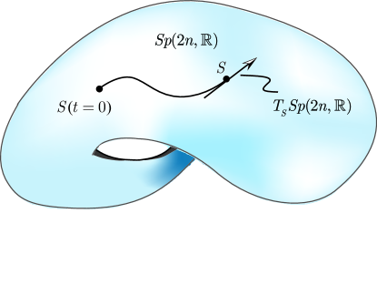
Figure 1: The space of the symplectic group $Sp\left(2n,\mathbb{R}\right)$ and the flow of $S$ on $Sp\left(2n,\mathbb{R}\right).$ At any given time, $J\tilde{A}S-SJA$ is tangential to $Sp\left(2n,\mathbb{R}\right),$ and the flow of $S$ according to Eq. (51) is always on $Sp\left(2n,\mathbb{R}\right).$

4 Proof of Theorem 1

We now apply the technique developed in Sec. 3 to prove Theorem 1. Our goal is to find a new coordinate system where the transformed Hamiltonian vanishes. This idea is identical to that in Hamilton-Jacobi theory. The goal is accomplished in two steps. First, we seek a coordinate transformation $\tilde{z}=Sz$ such that, in the $\tilde{z}$ coordinates, the Hamiltonian assumes the form

$$\bar{H}=\frac{1}{2}\tilde{z}^{\dagger}\tilde{A}\tilde{z}\,,\,\,\tilde{A}=\left(\begin{array}[]{cc}\mu(t)&0\\ 0&\mu(t)\end{array}\right)\,,$$ (55)

where $\mu(t)$ is a $n\times n$ matrix to be determined. Let the $2\times 2$ block form of $S$ is

$$S=\left(\begin{array}[]{cc}S_{1}&S_{2}\\ S_{3}&S_{4}\end{array}\right),$$ (56)

and split Eq. (51) into four $n\times n$ matrix equations,

$$\dot{S}_{1} =\mu S_{3}-S_{1}R^{\dagger}+S_{2}\kappa\,\,,$$ (57)

$$\dot{S}_{2} =\mu S_{4}-S_{1}m^{-1}+S_{2}R\,,$$ (58)

$$\dot{S}_{3} =-\mu S_{1}-S_{3}R^{\dagger}+S_{4}\kappa\,,$$ (59)

$$\dot{S}_{4} =-\mu S_{2}-S_{3}m^{-1}+S_{4}R\,.$$ (60)

Including $\mu(t),$ there are five $n\times n$ matrices unknown. The extra freedom is introduced by the to-be-determined $\mu(t)$. We choose $S_{2}\equiv 0$ to remove the freedom, and rename $S_{4}$ to be $w,$ i.e., $w\equiv S_{4}$. Equations (57)-(60) become

$$\dot{S}_{1} =\mu S_{3}-S_{1}R^{\dagger}\,,$$ (61)

$$S_{1} =\mu wm\,,$$ (62)

$$\dot{S}_{3} =-\mu S_{1}-S_{3}R^{\dagger}+w\kappa\,,$$ (63)

$$S_{3} =-\dot{w}m+wRm,$$ (64)

for matrices $S_{1}$, $S_{3}$, $w$ and $\mu$. Because $(S_{1},S_{2}=0,S_{3},S_{4}=w)$ describes a curve in $Sp\left(2n,\mathbb{R}\right),$ symplectic condition $S_{1}S_{4}^{\dagger}-S_{2}S_{3}^{\dagger}=I$ holds, which implies

$$S_{1}=w^{\dagger-1}\,.$$ (65)

From Eq. (62), we have

$$\mu=\left(wmw^{\dagger}\right)^{-1}.$$ (66)

Equation (61) is equivalent to another symplectic condition $S_{3}S_{4}^{\dagger}=S_{4}S_{3}^{\dagger}.$ Substituting Eqs. (64)-(66) into Eq. (63), we obtain the following matrix differential equation for the envelope matrix $w,$

$$\frac{d}{dt}\left(\frac{dw}{dt}m-wRm\right)+\frac{dw}{dt}mR^{\dagger}+w\left(\kappa-RmR^{\dagger}\right)-\left(w^{\dagger}wmw^{\dagger}\right)^{-1}=0\,.$$ (67)

This is the desired envelope equation in Theorem 1.

Once $w$ is solved for from the envelope equation, we can determine $S_{1}$ from Eq. (65) and $S_{3}$ from Eq. (64). In terms of the envelope matrix $w,$ the symplectic transformation $S$ and its inverse are given by

$$S =\left(\begin{array}[]{cc}w^{\dagger-1}&0\\ (wR-\dot{w})m&w\end{array}\right)\,,$$ (70)

$$S^{-1} =\left(\begin{array}[]{cc}w^{\dagger}&0\\ \left(w^{-1}\dot{w}-R\right)mw^{\dagger}&w^{-1}\end{array}\right)\,.$$ (73)

The second step is to use another coordinate transformation $\tilde{\tilde{z}}=P(t)\tilde{z}\,$ to transform $\tilde{H}$ into a vanishing Hamiltonian $\tilde{\tilde{H}}\equiv 0$ at all time, thereby rendering the dynamics trivial in the new coordinates. The determining equation for the transformation $P(t)$ is

$$\dot{P}=-PJ\tilde{A}=P\left(\begin{array}[]{cc}0&-\mu\\ \mu&0\end{array}\right)\,.$$ (74)

According to Lemma 3, the $P$ matrix satisfying Eq. (74) is symplectic because $J\tilde{A}\in sp(2n,\mathbb{R}).$ From $\mu=\mu^{\dagger}$, we know that $J\tilde{A}$ is also antisymmetric, i.e., $J\tilde{A}\in so(2n,\mathbb{R})$. Thus $J\tilde{A}\in sp(2n,\mathbb{R})\cap o(2n,\mathbb{R})$, and $P(t)$ is a curve in the group of $2n$-dimensional symplectic rotations, i.e., $P(t)\in Sp(2n,\mathbb{R})\cap O(2n,\mathbb{R})\backsimeq U(n)$, provided $P(t)$ starts from the group at $t=0.$ We call $P(t)$ the phase advance, an appropriate descriptor in light of the fact that $P(t)$ is a symplectic rotation. The Lie algebra element (infinitesimal generator) $-J\tilde{A}=\left(\begin{array}[]{cc}0&-\mu\\ \mu&0\end{array}\right)$ is the phase advance rate, and it is determined by the envelope matrix through Eq. (66). As an element in $Sp(2n,\mathbb{R})\cap O(2n,\mathbb{R})\backsimeq U(n)$, $P$ and its inverse must have the forms

$$P =\left(\begin{array}[]{cc}P_{1}&P_{2}\\ -P_{2}&P_{1}\end{array}\right)\,,$$ (77)

$$P^{-1} =P^{\dagger}=\left(\begin{array}[]{cc}P_{1}^{\dagger}&-P_{2}^{\dagger}\\ P_{2}^{\dagger}&P_{1}^{\dagger}\end{array}\right)\,.\,\,$$ (80)

Combining the two time-dependent canonical transformations, we have

$$\tilde{\tilde{z}}=G(t)z=P(t)S(t)z\,.$$ (81)

In the $\tilde{\tilde{z}}$ coordinates, because $\tilde{\tilde{H}}\equiv 0$, the dynamics is trivial, i.e., $\tilde{\tilde{z}}=const.$ This enables us to construct the solution map (8) as

$$M(t)=S^{-1}P^{-1}P_{0}S_{0}=\left(\begin{array}[]{cc}w^{\dagger}&0\\ \left(w^{-1}\dot{w}-R\right)mw^{\dagger}&w^{-1}\end{array}\right)P^{\dagger}\left(\begin{array}[]{cc}w^{-\dagger}&0\\ (wR-\dot{w})m&w\end{array}\right)_{0},$$ (82)

where subscript “0” denotes initial conditions at $t=0$, and $P_{0}$ is taken to be $I$ without loss of generality.

This completes the proof of Theorem (1).

The time-dependent canonical transformation can also be used to construct invariants of the dynamics. For any constant $2n\times 2n$ positive-definite matrix $\xi,$ the quantity

$$I_{\xi}=z^{\dagger}S^{\dagger}P^{\dagger}\xi PSz$$ (83)

is a constant of motion, since $\tilde{\tilde{z}}=PSz$ is a constant of motion. For the special case of $\xi=I,$ the phase advance $P$ in Eq. (83) drops out, and

$$I_{CS}\equiv z^{\dagger}S^{\dagger}Sz=z^{\dagger}\left(\begin{array}[]{cc}\gamma&\alpha\\ \alpha^{T}&\beta\end{array}\right)z\,,$$ (84)

where $\alpha,$ $\beta,$ and $\gamma$ are $2\times 2$ matrices defined by

$$\alpha \equiv w^{\dagger}S_{3}\,,$$ (85)

$$\beta \equiv w^{\dagger}w\,,$$ (86)

$$\gamma \equiv S_{3}^{\dagger}S_{3}+w^{-1}w^{-\dagger}\,.$$ (87)

Here, we use $I_{CS}$ to denote this special invariant because it is the invariant that generalizes the Courant-Snyder invariant (Courant and Snyder, 1958) (or Lewis invariant (Lewis, 1968; Lewis and Riesenfeld, 1969)) for one degree of freedom in Eq. (35).

5 Normal forms for stable symplectic matrices

In this section, normal forms for stable symplectic matrices are developed. We first list necessary definitions and facts related to the eigenvalues, eigenvector spaces, and root-vector spaces of symplectic matrices. Lemmas 4-10 are given without proofs, which can be found in the textbooks by Long (Long, 2002), Ekeland (Ekeland, 1990), and Yakubovich and Starzhinskii (Yakubovich and Starzhinskii, 1975).

The set of eigenvalues of a matrix $M$ is denoted by

$$\sigma(M)=\left\{\lambda|\det(I\lambda-M)=0\right\},$$ (88)

and the unit circle on the complex plane $\mathbb{C}$ is denoted by $U.$

Lemma 4.

For a symplectic matrix $M\in Sp(2n,\mathbb{R}),$ its eigenvalue space $\sigma(M)$ is symmetric with respect to the real axis and the unit circle $U$, i.e., if $\lambda_{0}\in\sigma(M),$ then $\bar{\lambda}_{0},$$\lambda_{0}^{-1}\in\sigma(M).$

The symmetry of $\sigma(M)$ with respect to the real axis is not specific to symplectic matrices. It is true for all real matrices. For a $\lambda\in\sigma(M)$, denote the eigenvector space by $V_{\lambda}(M)$ and the root-vector space by $E_{\lambda}(M)$,

$$V_{\lambda}(M) \equiv\textrm{ker}(M-\lambda I)\subset\mathbb{C}^{2n},$$ (89)

$$E_{\lambda}(M) \equiv\cup_{k\geq 1}\textrm{ker}(M-\lambda I)^{k}\subset\mathbb{C}^{2n}.$$ (90)

The dimension of $V_{\lambda}(M)$ is the geometric multiplicity of $\lambda,$ denoted by $Mult_{G\lambda}(M)$, and the dimension of $E_{\lambda}(M)$ is the algebraic multiplicity of $\lambda,$ denoted by $Mult_{A\lambda}(M)$. A subspace $V\subset\mathbb{C}^{2n}$ is an invariant subspace if $MV\subset\mathbb{C}^{2n}$. An invariant subspace is irreducible if it is not a direct sum of two non-trivial invariant subspaces. For every $\lambda$, the root-vector space $E_{\lambda}(M)$ is an invariant subspace, and a direct sum of irreducible subspaces. On the other hand, every irreducible subspace of $M$ is contained in one of the root-vector spaces. An eigenvalue $\lambda$ is simple if $Mult_{G\lambda}(M)=$$Mult_{A\lambda}(M)=1$. An eigenvalue $\lambda$ is semi-simple, if $E_{\lambda}(M)$ is a direct sum of one-dimensional irreducible invariant subspaces only, which is equivalent to that all elementary divisors of $\lambda$ are simple. When $\lambda$ is semi-simple, the eigenvector space $V_{\lambda}(M)$ is at its maximum dimension. It has fulfilled its obligation to provide enough eigenvectors for the purpose of diagonalizing $M$, even though $Mult_{G\lambda}(M)=$$Mult_{A\lambda}(M)$ could be larger than $1$. If $M$ is not diagonalizable, other eigenvalues have to be blamed.

For any two vectors $\psi$ and $\phi$ in $\mathbb{C}^{2n},$ the Krein product is

$$\left\langle\psi,\phi\right\rangle_{G}\equiv\left\langle G\psi,\phi\right\rangle=-\phi^{*}iJ\psi,$$ (91)

where $G=-iJ$ and $\phi^{*}=\bar{\phi}^{\dagger}$ is the Hermitian transpose of $\phi.$ Obviously,

$$\left\langle\psi,\phi\right\rangle_{G}=\overline{\left\langle\phi,\psi\right\rangle_{G}}\,.$$ (92)

For a vector $\psi$ in $\mathbb{C}^{2n},$ it Krein amplitude is defined to be $\left\langle\psi,\psi\right\rangle_{G}$, the sign of which is the Krein signature of $\psi.$

Two vectors $\psi$ and $\phi$ in $\mathbb{C}^{2n}$ are G-orthogonal if $\left\langle\psi,\phi\right\rangle_{G}=0.$ Two subspaces $V_{1}$ and $V_{1}$ are G-orthogonal if $\left\langle\psi_{1},\psi_{2}\right\rangle_{G}=0$ for any $\psi_{1}\in V_{1}$ and $\psi_{2}\in V_{2}.$ A subspace is G-isotropic if it is G-orthogonal to itself.

Krein amplitude has a clear physical meaning. The one-period solution map $M(T)$ according to Eq. (82) can be expressed as

$$M(T)=\exp(J\hat{A}T)\,,$$ (93)

where $\hat{A}$ is an effective matrix representing the averaged effect by $A$ in one period. In physics, an eigenvector $\psi\in V_{\lambda}(M)$ is known as an eigenmode, and the jargon of eigen-frequency $\omega$, defined by $\exp(-i\omega T)=\lambda$, is preferred. An eigenmode $\psi$ of $M(T)$ is also an eigenmode of $J\hat{A}$,

$$J\hat{A}\psi=-i\omega\psi\,.$$ (94)

The Krein amplitude of $\psi$ is

$$\left\langle\psi,\psi\right\rangle_{G}=-i\psi^{*}J\psi=-\frac{\psi^{*}\hat{A}\psi}{\omega}=-2\frac{\hat{H}}{\omega}\,,$$ (95)

which is proportional to the negative of the action of the eigenmode, i.e., the time integral of the effective energy over one period. Because the ratio between $\left\langle\psi,\psi\right\rangle_{G}$ and $\hat{H}/\omega$ is an unimportant constant, we can identify the Krein amplitude with the action of the eigenmode (Zhang et al., 2016, 2017, 2018).

The following lemma gives a necessary condition for an eigenvalue on the unit circle to be non-semi-simple.

Lemma 5.

For a $\lambda\in\sigma(M)\cap U$ with at least one multiple elementary divisor, there exists $\psi\in E_{\lambda}(M)$ such that $\left\langle\psi,\psi\right\rangle_{G}=0$ .

Lemma 6.

For two eigenvalues $\lambda$ and $\mu$, the eigenvector spaces $V_{\lambda}$ and $V_{\mu}$ are G-orthogonal if $\lambda\bar{\mu}\neq 1.$

It is remarkable that the G-orthogonality can be established for the root-vector spaces as well.

Lemma 7.

For two eigenvalues $\lambda$ and $\mu$, the root-vector spaces $E_{\lambda}$ and $E_{\mu}$ are G-orthogonal if $\lambda\bar{\mu}\neq 1.$

Lemma 7 implies for any $\lambda\in\sigma(M)\cap U,$ $E_{\lambda}$ is G-orthogonal to $E_{\mu}$ when $\mu\neq\lambda.$ As a consequence, $\mathbb{C}^{2n}$ has the following G-orthogonal decomposition (Long, 2002)

$$\mathbb{C}^{2n} =\left(\oplus_{\lambda\in\sigma(M)\cap U}E_{\lambda}(M)\right)\oplus F(M)\,,$$ (96)

where

$$F(M)=\oplus_{\lambda\in\sigma(M)\backslash U}E_{\lambda}(M)\,$$ (97)

is the direct sum of the root-vector spaces for all eigenvalues off the unit circle. Note that root-vector spaces for different eigenvalues off the unit circle are not G-orthogonal in general.

Lemma 8.

For a $\lambda\in\sigma(M)\cap U$, $E_{\lambda}(M)$ is an invariant subspace of $G=-iJ.$ Furthermore, the restriction of $G$ on $E_{\lambda}(M)$ is non-degenerate, i.e., for $x$ and $y$ in $E_{\lambda}(M)$, $\left\langle x,y\right\rangle_{G}=0$ for all $y$ implies that $x=0.$

As an operator on $\mathbb{C}^{2n}$, $G=-iJ$ is Hermitian, i.e., $\left(-iJ\right)^{*}=-iJ$. It is also non-degenerate because $\text{det}(G)\neq 0$. Since a Hermitian matrix is diagonalizable and its eigenvalues are all real, there exists a G-orthogonal basis for $\mathbb{C}^{2n}$.

By Lemma 8, the restriction of $G$ on $E_{\lambda}(M)$ for $\lambda\in\sigma(M)\cap U$ is a non-degenerate Hermitian operator, which implies $G|_{E_{\lambda}(M)}$ is diagonalizable with non-zero eigenvalues. Similar to the situation for $\mathbb{C}^{2n}$, the space of $E_{\lambda}(M)$ admits a G-orthogonal base. Let the dimension of of $E_{\lambda}(M)$ is $m$, and $p$ and $q$ are the numbers of positive and negative eigenvalues of $G|_{E_{\lambda}(M)}$ respectively. The pair $(p,q)$ is known as the Krein type of $\lambda.$ Obviously, $p+q=m.$ If $q=0$, $\lambda$ is Krein-positive, and if $p=0$, $\lambda$ is Krein-negative. An eigenvalue $\lambda$ is Krein-definite, if it is either Krein-positive or Krein-negative. Otherwise, $\lambda$ is Krein-indefinite or of mixed type.

Lemma 9.

For a $\lambda\in\sigma(M)\cap U$ and any $P\in Sp(2n,\mathbb{R}),$ the geometric and algebraic multiplicities and Krein type of $\lambda$ are identical for $P^{-1}MP$ and $M.$

Lemma 10.

(a) For any $x\in\mathbb{C}^{2n}$, $\left\langle Gx,x\right\rangle=-\left\langle G\bar{x},\bar{x}\right\rangle.$

(b) If $\lambda\in\sigma(M)\cap U$ has Krein type $(p,q)$, then $\bar{\lambda}$ has Krein type $(q,p)$. In particular, if $1$ or $-1$ is an eigenvalue of $M$, its Krein type is $(p,p)$ for some $p\in\mathbb{N}$.

The $\diamond$-product of two square matrices introduced by Long (Long, 2002) is an indispensable tool in the manipulations of symplectic matrices. Let $M_{1}$ be a $2i\times 2i$ matrix and $M_{2}$ a $2j\times 2j$ matrix in the square block form,

$$M_{1}=\left(\begin{array}[]{cc}A_{1}&B_{1}\\ C_{1}&D_{1}\end{array}\right)\,,\,\,\,\,M_{2}=\left(\begin{array}[]{cc}A_{2}&B_{2}\\ C_{2}&D_{2}\end{array}\right)\,.$$ (98)

The $\diamond$-product of $M_{1}$ and $M_{2}$ is defined to be a $2(i+j)\times 2(i+j)$ matrix as

$$M_{1}\diamond M_{2}=\left(\begin{array}[]{cccc}A_{1}&0&B_{1}&0\\ 0&A_{2}&0&B_{2}\\ C_{1}&0&D_{1}&0\\ 0&C_{2}&0&D_{2}\end{array}\right)\,.$$ (99)

The $\diamond$-product defined here is compatible with the standard symplectic matrix defined in Eq. (4). The $\diamond$-product of two symplectic matrices is symplectic (Long, 2002). It can be viewed as a direct sum of two matrix vectors to form a matrix vector in higher dimension. The following theorem is the main result of this section, which establishes the normal form for a stable symplectic matrix.

Theorem 11.

For a symplectic matrix $M\in Sp(2n,\mathbb{R})$, it is stable iff it is similar to a direct sum of elements in $SO(2,\mathbb{R})$ by a symplectic matrix, i.e., there exist a $N=R(\theta_{1})\diamond R(\theta_{2})...\diamond R(\theta_{n})$ and a $F\in Sp(2n,\mathbb{R})$ such that

$$M=FNF^{-1},$$ (100)

where $\theta_{j}\in\mathbb{R}$ and

$$R(\theta_{j})=\left(\begin{array}[]{cc}\cos\theta_{j}&\sin\theta_{j}\\ -\sin\theta_{j}&\cos\theta_{j}\end{array}\right)\in SO(2,\mathbb{R}).$$ (101)

Proof.

Recall that stability of $M$ means that $M$ is diagonalizable and all eigenvalues of $M$ locate on the unit circle $U$ of the complex plane. It is straightforward to verify that $N=R(\theta_{1})\diamond R(\theta_{2})...\diamond R(\theta_{n})\in Sp(2n,\mathbb{R})\cap O(2n,\mathbb{R})\backsimeq U(n).$ Since a unitary matrix is stable, the sufficiency is obvious.

For necessity, assume that $M\in Sp(2n,\mathbb{R})$ is stable. First, let’s construct a G-orthonormal basis $(\psi_{l},\psi_{-l})\,,\,l=1,2,...,n,$ for $\mathbb{C}^{2n}$, which by definition satisfies the following conditions for $1\leq l,m\leq n$,

$$M\psi_{l} =\lambda_{l}\psi_{l}\,,$$ (102)

$$\psi_{-l} =\bar{\psi}_{l}\,,$$ (103)

$$\left\langle G\psi_{l},\psi_{m}\right\rangle =\delta_{lm\,,}$$ (104)

$$\left\langle G\psi_{-l},\psi_{-m}\right\rangle =-\delta_{lm\,,}$$ (105)

$$\left\langle G\psi_{l},\psi_{-m}\right\rangle =0\,,$$ (106)

where $\left(\lambda_{l},\psi_{l}\right)$ is a pair of eigenvalue and eigenvector, so is $\left(\bar{\lambda}_{l},\psi_{-l}\right)$. Thus this G-orthonormal basis $(\psi_{l},\psi_{-l})\,\,(l=1,2,...,n)$ for $\mathbb{C}^{2n}$ consists of eigenvectors of $M$, with appropriately chosen labels. There are in total $2n$ eigenvectors. Because $M$ is stable, every eigenvalue of $M$ is on the unit circle $U$ and is either simple or semi-simple, and for every $\lambda\in\sigma(M)$, the eigenvector space $V_{\lambda}(M)$ is identical to the root-vector space $E_{\lambda}(M).$ The simple and semi-simple cases need to be treated differently.

Case a). For a simple eigenvalue $\lambda$ on $U$, $V_{\lambda}(M)=E_{\lambda}(M)$ is one-dimensional. Denote the eigenvector by $\psi_{\lambda}$. According to Lemma 7, $\psi_{\lambda}$ is G-orthogonal to any other eigenvector or root-vector of $M.$ By Lemma 8, $\left\langle\psi_{\lambda},\psi_{\lambda}\right\rangle_{G}\neq 0.$ Without losing generality, we can let $\left\langle\psi_{\lambda},\psi_{\lambda}\right\rangle_{G}=1$ or $-1$. Now, for every simple $\lambda$ on $U$, $\bar{\lambda}$ is in $\sigma(M)\cap U$ and $\bar{\lambda}\neq\lambda$. Furthermore, $\bar{\lambda}$ is also simple with opposition Krein signature, and the corresponding eigenvector $\psi_{\bar{\lambda}}$ is G-orthogonal to all other eigenvectors or root-vectors. All the eigenvectors corresponding to simple eigenvalues pair up nicely in this manner. It is natural to denote them by $\left(\psi_{l},\psi_{-l}\right),\,1\leq l\leq n_{s}$, where $2n_{s}$ is the total number of simple eigenvalues and $l$ is the index for the simple eigenvalues. The pair of eigenvectors $\left(\psi_{l},\psi_{-l}\right)$ correspond to the pair of eigenvalues $(\lambda_{l},\bar{\lambda}_{l}),$ where $\psi_{l}$ is the eigenvector with positive Krein signature, and $\psi_{-l}$ with the negative Krein signature. Therefore, $\left(\psi_{l},\psi_{-l}\right),\,1\leq l\leq n_{s}$, form a G-orthonormal basis satisfying Eqs. (102)-(106), for the subspace spanned by the eigenvectors of simple eigenvalues on the unit circle $U.$

Case b). For a semi-simple eigenvalue $\mu$ on $U$, the subspace $V_{\mu}(M)=E_{\mu}(M)$ is two-dimensional or higher. Since $G$ is Hermitian on $E_{\mu}(M),$ it can be diagonalized using a proper basis $\psi_{\mu}^{i},$ $i=1,...,m_{\mu}$, on $E_{\mu}(M),$ where $m_{\mu}$ is the multiplicity of $\mu.$ By Lemma 8, the restriction of $G$ on $E_{\mu}(M)$ is non-degenerate. The eigenvalues of $G$ is either positive or negative. Let the Krein type of $\mu$ is $(p,q)$ with $p+q=m_{\mu}.$ Lemma 10 asserts that the Krein type of $\bar{\mu}$ is $(q,p),$ with $\psi_{\bar{\mu}}^{i}=\bar{\psi}_{\mu}^{i}.$

Case b1). When $\mu\neq\pm 1,$ $\mu\neq\bar{\mu}$ and $E_{\mu}(M)$ is G-orthogonal to $E_{\bar{\mu}}(M).$ We can thus pair up $\psi_{\mu}^{i}$ and $\psi_{\bar{\mu}}^{i}$ for $i=1,...,m_{\mu}$ to form a G-orthonormal basis satisfying Eqs. (102)-(106) for the subspace $E_{\mu}(M)\oplus E_{\bar{\mu}}(M).$

Case b2). When $\mu=\pm 1,$ $E_{\mu}(M)=E_{\bar{\mu}}(M)$ and $p=q=m_{\mu}/2$. In this case, we can construct a G-orthonormal base of $E_{\mu}(M)$ in the following way. Let $\psi_{\mu}^{i},$ $i=1,...,p,$ be eigenvectors with positive Krein signatures. Then according to Lemma 10, $\bar{\psi}_{\mu}^{i},$ $i=1,...,p,$ will have negative Krein signatures. Note also that $\left(\psi_{\mu}^{i},\bar{\psi}_{\mu}^{i}\right),$ $i=1,...,p$, diagonalize $G$ on $E_{\mu}(M).$ Thus, the pairs $\left(\psi_{\mu}^{i},\bar{\psi}_{\mu}^{i}\right),$ $i=1,...,p$, make up a G-orthonormal base satisfying Eqs. (102)-(106) for the subspace $E_{\mu}(M)=E_{\bar{\mu}}(M)$.

Assembling the eigenvector pairs from Cases a), b1), b2) in the order presented, we obtain the G-orthonormal base $(\psi_{l},\psi_{-l}),\,l=1,2,...,n,$ for $\mathbb{C}^{2n}$ satisfying Eqs. (102)-(106). Note that the eigenvalues $\lambda_{l}$ $(1\leq l\leq n_{s})$ are simple and distinct, whereas the eigenvalues $\lambda_{l}$ $(n_{s}+1\leq l\leq n)$ are semi-simple, and each eigenvalue may appear several times in the sequence.

Now, we explicitly build the normal form of Eq. (100) using the G-orthonormal base $(\psi_{l},\psi_{-l}),\,l=1,2,...,n$. Let

$$\psi_{l}=\xi_{l}+\sqrt{-1}\eta_{l}\,,\,\,\lambda_{l}=c_{l}+\sqrt{-1}s_{l}\,,$$ (107)

where $\xi_{l}$, $\eta_{l}\in\mathbb{R}^{2n}$, $c_{l}=\cos\theta_{l},$ $s_{l}=\sin\theta_{l},$ and $0\leq\theta_{l}<2\pi$. In terms of this set of real variables, $M\psi_{l}=\lambda_{l}\psi_{l}$ is

$$M\xi_{l} =c_{l}\xi_{l}-s_{l}\eta_{l}\,,$$ (108)

$$M\eta_{l} =c_{l}\eta_{l}+s_{l}\xi_{l}\,.$$ (109)

The G-orthonormal conditions (104)-(106) are equivalent to

$$\left\langle J\xi_{l},\xi_{m}\right\rangle =0\,,$$ (110)

$$\left\langle J\eta_{l},\eta_{m}\right\rangle =0\,,$$ (111)

$$\left\langle J\xi_{l},\eta_{m}\right\rangle =\eta_{m}^{\dagger}J\xi_{l}=-\delta_{lm}/2\,,$$ (112)

$$\left\langle J\eta_{l},\xi_{m}\right\rangle =\xi_{m}^{\dagger}J\eta_{l}=\delta_{lm}/2\,.$$ (113)

We now prove that the matrix $F$ in Eq. (100) in given by

$$F=\sqrt{2}\left(\xi_{1},\xi_{2},...,\xi_{n},\eta_{1},\eta_{2},...,\eta_{n}\right)\,.$$ (114)

The fact that $F\in Sp(2n,\mathbb{R})$ is shown by direct calculation,

$$F^{\dagger}JF =2\left(\begin{array}[]{c}\xi_{1}^{\dagger}\\ \vdots\\ \xi_{n}^{\dagger}\\ \eta_{1}^{\dagger}\\ \vdots\\ \eta_{n}^{\dagger}\end{array}\right)J\left(\xi_{1},\xi_{2},...,\xi_{n},\eta_{1},\eta_{2},...,\eta_{n}\right)$$ (121)

$$=2\left(\begin{array}[]{cccccc}\xi_{1}^{\dagger}J\xi_{1}&\ldots&\xi_{1}^{\dagger}J\xi_{n}&\xi_{1}^{\dagger}J\eta_{1}&\cdots&\xi_{1}^{\dagger}J\eta_{n}\\ \vdots&\ddots&\vdots&\vdots&\ddots&\vdots\\ \xi_{1}^{\dagger}J\xi_{1}&\ldots&\xi_{1}^{\dagger}J\xi_{n}&\xi_{1}^{\dagger}J\eta_{1}&\cdots&\xi_{1}^{\dagger}J\eta_{n}\\ \eta_{1}^{\dagger}J\xi_{1}&\ldots&\eta_{1}^{\dagger}J\xi_{n}&\eta_{1}^{\dagger}J\eta_{1}&\cdots&\eta_{1}^{\dagger}J\eta_{n}\\ \vdots&\ddots&\vdots&\vdots&\ddots&\vdots\\ \eta_{n}^{\dagger}J\xi_{1}&\ldots&\eta_{n}^{\dagger}J\xi_{n}&\eta_{n}^{\dagger}J\eta_{1}&\cdots&\eta_{n}^{\dagger}J\eta_{n}\end{array}\right)$$ (128)

$$=J\,,$$ (129)

where Eqs. (110)-(113) are used in the last equal sign. The last step is to show that $N=F^{-1}MF=-JF^{\dagger}JMF$ is of the form $R(\theta_{1})\diamond R(\theta_{2})...\diamond R(\theta_{n})$, again by direct calculation. From Eqs. (108) and (109), we have

$$MF =\sqrt{2}\left(M\xi_{1},...,M\xi_{n},M\eta_{1},...,M\eta_{n}\right)$$

$$=\sqrt{2}\left(c_{1}\xi_{1}-s_{1}\eta_{1},...,c_{n}\xi_{n}-s_{n}\eta_{n},s_{1}\xi_{1}+c_{1}\eta_{1},...,s_{n}\xi_{n}+c_{n}\eta_{n}\right)\,.$$ (130)

Then,

$$N =-JF^{\dagger}JMF$$

$$=-2J\left(\begin{array}[]{c}\xi_{1}^{\dagger}\\ \vdots\\ \xi_{n}^{\dagger}\\ \eta_{1}^{\dagger}\\ \vdots\\ \eta_{n}^{\dagger}\end{array}\right)J\left(c_{1}\xi_{1}-s_{1}\eta_{1},...,c_{n}\xi_{n}-s_{n}\eta_{n},s_{1}\xi_{1}+c_{1}\eta_{1},...,s_{n}\xi_{n}+c_{n}\eta_{n}\right)$$ (137)

$$=-2J\left(\begin{array}[]{cccccc}\xi_{1}^{\dagger}J\left(\xi_{1}c_{1}-\eta_{1}s_{1}\right)&\ldots&\xi_{1}^{\dagger}J\left(\xi_{n}c_{n}-\eta_{n}s_{n}\right)&\xi_{1}^{\dagger}J\left(\xi_{1}s_{1}+\eta_{1}c_{1}\right)&\ldots&\xi_{1}^{\dagger}J\left(\xi_{n}s_{n}+\eta_{n}c_{n}\right)\\ \vdots&\ddots&\vdots&\vdots&\ddots&\vdots\\ \xi_{n}^{\dagger}J\left(\xi_{1}c_{1}-\eta_{1}s_{1}\right)&\ldots&\xi_{n}^{\dagger}J\left(\xi_{n}c_{n}-\eta_{n}s_{n}\right)&\xi_{n}^{\dagger}J\left(\xi_{1}s_{1}+\eta_{1}c_{1}\right)&\ldots&\xi_{n}^{\dagger}J\left(\xi_{n}s_{n}+\eta_{n}c_{n}\right)\\ \eta_{1}^{\dagger}J\left(\xi_{1}c_{1}-\eta_{1}s_{1}\right)&\ldots&\eta_{1}^{\dagger}J\left(\xi_{n}c_{n}-\eta_{n}s_{n}\right)&\eta_{1}^{\dagger}J\left(\xi_{1}s_{1}+\eta_{1}c_{1}\right)&\ldots&\eta_{1}^{\dagger}J\left(\xi_{n}s_{n}+\eta_{n}c_{n}\right)\\ \vdots&\ddots&\vdots&\vdots&\ddots&\vdots\\ \eta_{n}^{\dagger}J\left(\xi_{1}c_{1}-\eta_{1}s_{1}\right)&\ldots&\eta_{n}^{\dagger}J\left(\xi_{n}c_{n}-\eta_{n}s_{n}\right)&\eta_{n}^{\dagger}J\left(\xi_{1}s_{1}+\eta_{1}c_{1}\right)&\ldots&\eta_{n}^{\dagger}J\left(\xi_{n}s_{n}+\eta_{n}c_{n}\right)\end{array}\right)$$ (144)

$$=-J\left(\begin{array}[]{cccccc}-s_{1}&0&0&c_{1}&0&0\\ 0&\ddots&0&0&\ddots&0\\ 0&0&-s_{n}&0&0&c_{n}\\ -c_{1}&0&0&-s_{1}&0&0\\ 0&\ddots&&0&\ddots&0\\ 0&0&-c_{n}&0&0&-s_{n}\end{array}\right)=\left(\begin{array}[]{cccccc}c_{1}&0&0&s_{1}&0&0\\ 0&\ddots&0&0&\ddots&0\\ 0&0&c_{n}&0&0&s_{n}\\ -s_{1}&0&0&c_{1}&0&0\\ 0&\ddots&0&0&\ddots&0\\ 0&0&-s_{n}&0&0&c_{n}\end{array}\right)$$ (157)

$$=R(\theta_{1})\diamond...\diamond R(\theta_{n})\,,$$ (158)

where Eqs. (110)-(113) are used again in the 4th equal sign. ∎

6 Horizontal polar decomposition of symplectic matrices

In this section, we develop the second tool, horizontal polar decomposition of symplectic matrices, for the purpose of proving Theorem 2. Judging from its name, horizontal polar decomposition bears some resemblance to the familiar matrix polar decomposition. The adjective “horizontal” is of course related to the natures of even-dimensional symplectic vector spaces. To understand its construction, we start from Lagrangian subspaces (de Gosson, 2006).

The standard symplectic matrix $J$ given by Eq. (4) defines a 2-form on $\mathbb{R}^{2n}$,

$$\sigma(z_{1},z_{2})=z_{2}^{\dagger}Jz_{1}\,.$$ (159)

The space $\mathbb{R}^{2n}$ equipped with $\sigma$ is called the standard symplectic space $\left(\mathbb{R}^{2n},\sigma\right).$

Recall that a subspace $l\subset$$\left(\mathbb{R}^{2n},\sigma\right)$ is called a Lagrangian plane or Lagrangian subspace if it has dimension $n$ and $\sigma(z_{1},z_{2})=0$ for all $z_{1},z_{2}\in l.$ The space of all Lagrangian planes is the Lagrangian Grassmannian denoted by $Lag(2n).$ Two special Lagrangian planes are the horizontal plan $l_{x}=\mathbb{R}^{n}\times 0$ and the vertical plane $l_{p}=0\times\mathbb{R}^{n}$. Symplectic matrices act on $Lag(2n)$, i.e., for $M\in Sp(2n,\mathbb{R})$ and $l\in Lag(2n),$ $Ml\in Lag(2n).$ The following lemma highlights the role of the subgroup $Sp(2n,\mathbb{R})\cap O(2n,\mathbb{R})\backsimeq U(n)$ in the action of symplectic group on the Lagrangian Grassmannian.

Lemma 12.

The action of $Sp(2n,\mathbb{R})\cap O(2n,\mathbb{R})\backsimeq U(n)$ on $Lag(2n)$ is transitive, i.e., for every pairs of $\left\{l_{1},l_{2}\right\}\subset Lag(2n),$ there exists a $u\in Sp(2n,\mathbb{R})\cap O(2n,\mathbb{R})\backsimeq U(n)$ such that $l_{2}=ul_{1}.$

The lemma can be proved by establishing othor-symplectic bases for $\left(\mathbb{R}^{2n},\sigma\right)$ over $l_{1}$ and $l_{2}$. See Ref. (de Gosson, 2006) for details. For a given $l\in Lag(2n),$ all $S\in Sp(2n,\mathbb{R})$ that satisfy $Sl=l$ form a subgroup. It is called the stabilizer or isotropy subgroup of $l,$ and is denoted by $St(l).$ For the vertical Lagrangian subsapce $l_{p}=0\times\mathbb{R}^{n},$ its stabilizer must be of the form

$$S=\left(\begin{array}[]{cc}L&0\\ Q&D\end{array}\right)\,.$$ (160)

Furthermore, the symplectic condition requires that $L^{\dagger}Q$ is symmetric and $D=L^{\dagger-1}$, which reduce $S$ to

$$S=\left(\begin{array}[]{cc}L&0\\ Q&L^{\dagger-1}\end{array}\right)=\left(\begin{array}[]{cc}I&0\\ P&I\end{array}\right)\left(\begin{array}[]{cc}L&0\\ 0&L^{\dagger-1}\end{array}\right)\,,$$ (161)

where $P=QL^{-1}$ is symmetric. For any $M\in Sp(2n,\mathbb{R})$, let’s consider the Lagrangian subspaces $M^{-1}l_{p}$ and $l_{p}$. By Lemma 12, there must exit a $u\in Sp(2n,\mathbb{R})\cap O(2n,\mathbb{R})\backsimeq U(n)$ such that $M^{-1}l_{p}=ul_{p},$ which implies $u^{-1}M^{-1}\in St(l_{p}),$ or, there must exist a $S\in St(l_{p})$ such that $M^{-1}=uS.$ Equivalently, there must exist a $u^{\prime}\in Sp(2n,\mathbb{R})\cap O(2n,\mathbb{R})\backsimeq U(n)$ and a $S^{\prime}\in St(l_{p})$ such that $M=u^{\prime}S^{\prime}.$ Since $S^{\prime}$ must have the form in Eq. (161), we conclude that $M$ can always be decomposed as

$$M=\left(\begin{array}[]{cc}X&Y\\ -Y&X\end{array}\right)\left(\begin{array}[]{cc}L&0\\ Q&L^{\dagger-1}\end{array}\right)\,,$$ (162)

where $L^{\dagger}Q$ is symmetric. Following de Gosson (de Gosson, 2006), this decomposition is called pre-Iwasawa decomposition. The justification of this terminology will be given shortly. One important fact to realize is that the pre-Iwasawa decomposition of a symplectic matrix by $Sp(2n,\mathbb{R})\cap O(2n,\mathbb{R})\backsimeq U(n)$ and $St(l_{p})$ is not unique. For any given pre-Iwasawa decomposition $M=uS$ with $u\in U(n)$ and $S\in St(l_{p}),$ a family of decompositions can be constructed using $O(n,\mathbb{R})$ as $M=u^{\prime}S^{\prime},$ where

$$u^{\prime} =ug^{-1}\in Sp(2n,\mathbb{R})\cap O(2n,\mathbb{R})\backsimeq U(n)\,,$$ (163)

$$S^{\prime} =gS\in St(l_{p})\,,$$ (164)

$$g =\left(\begin{array}[]{cc}c&0\\ 0&c\end{array}\right)\,,\,\,\,c\in O(n,\mathbb{R})\,.$$ (167)

This family of pre-Iwasawa decompositions is generated by a $O(n,\mathbb{R})$ gauge freedom. One way to fix the gauge freedom is to demand $L$ to be positive-definite. Different choice of $c\in O(n,\mathbb{R})$ in the family of pre-Iwasawa decomposition corresponds to different $L$ in Eq. (162). Since the polar decomposition of a matrix into a positive matrix and a rotation is unique, the pre-Iwasawa decomposition is unique when the $n\times n$ matrix $L$ is required to be positive-definite. Because $L$ corresponds to the horizontal components of $z$, such a requirement demands horizontal positive-definiteness. We call this special pre-Iwasawa decomposition horizontal polar decomposition of a symplectic matrix. Vertical polar decomposition can be defined similarly.

Theorem 13.

(Horizontal polar decomposition) A symplectic matrix $M\in Sp(2n,\mathbb{R})$ can be uniquely decomposed as

$$M=\left(\begin{array}[]{cc}X&Y\\ -Y&X\end{array}\right)\left(\begin{array}[]{cc}L&0\\ Q&L^{-1}\end{array}\right)\,,$$ (168)

where $\left(\begin{array}[]{cc}X&Y\\ -Y&X\end{array}\right)\in Sp(2n,\mathbb{R})\cap O(2n,\mathbb{R})\backsimeq U(n)$, $L$ is positive-definite, and $L^{\dagger}Q$ is symmetric.

Proof.

The existence of the decomposition has been established by the pre-Iwasawa decomposition derived above. We only need to prove the uniqueness. Assume there are two horizontal polar decompositions, $M=uS=u^{\prime}S^{\prime}.$ We have $SS^{\prime-1}=u^{-1}u^{\prime}\in Sp(2n,\mathbb{R})\cap O(2n,\mathbb{R})\backsimeq U(n),$ or,

$$\left(\begin{array}[]{cc}L&0\\ Q&L^{-1}\end{array}\right)\left(\begin{array}[]{cc}L^{\prime-1}&0\\ -Q^{\prime\dagger}&L^{\prime}\end{array}\right)=\left(\begin{array}[]{cc}LL^{\prime-1}&0\\ QL^{\prime-1}-L^{-1}Q^{\prime\dagger}&L^{-1}L^{\prime}\end{array}\right)=\left(\begin{array}[]{cc}A&B\\ -B&A\end{array}\right)\,.$$ (169)

Then, $LL^{\prime-1}=L^{-1}L^{\prime}$, or, $L^{2}=L^{\prime 2}.$ Since $L$ and $L^{\prime}$ are positive-definite, $L=L^{\prime}.$ In addition, $QL^{\prime-1}=L^{-1}Q^{\prime\dagger},$ i.e., $LQ=Q^{\prime\dagger}L^{\prime},$ which gives $Q=Q^{\prime},$ considering the symplectic condition $Q^{\prime\dagger}L^{\prime}=L^{\prime}Q^{\prime}.$ ∎

Similar to the standard polar decomposition of an invertible square matrix, there is an explicit formula for the horizontal polar decomposition of a symplectic matrix in terms of its block components.

Corollary 14.

The horizontal polar decomposition of a symplectic matrix

$$M=\left(\begin{array}[]{cc}A&B\\ C&D\end{array}\right)$$ (170)

is given by

$$M =\left(\begin{array}[]{cc}X&Y\\ -Y&X\end{array}\right)\left(\begin{array}[]{cc}L&0\\ Q&L^{-1}\end{array}\right)\,,$$ (175)

$$X =DL\,,\,\,\,Y=BL\,,$$ (176)

$$L =\left(B^{\dagger}B+D^{\dagger}D\right)^{-1/2}\,,$$ (177)

$$Q =L(B^{\dagger}A+D^{\dagger}C)\,.$$ (178)

Proof.

Carrying out the matrix multiplication on the right-hand-side of Eq. (175), we have, block by block,

$$A =XL+YQ\,,$$ (179)

$$C =-YL+XQ$$ (180)

$$B =YL^{-1}\,,\,\,\,D=XL^{-1}\,.$$ (181)

From Eq. (181), we have Eq. (176) and

$$B^{\dagger}B+D^{\dagger}D=L^{-1}(X^{\dagger}X+Y^{\dagger}Y)L^{-1}=L^{-2},$$ (182)

where use is made of $X^{\dagger}X+Y^{\dagger}Y=I.$ Since $L$ is positive-definite, it’s square-root is unique, and Eq. (177) follows. Equations (176) and (177) confirm that $\left(\begin{array}[]{cc}X&Y\\ -Y&X\end{array}\right)$ indeed belongs to $U(n).$ Summing $X^{\dagger}$Eq. (180) and $Y^{\dagger}$Eq. (179) gives

$$X^{\dagger}C+Y^{\dagger}A=\left(Y^{\dagger}X-X^{\dagger}Y\right)L+\left(Y^{\dagger}Y+X^{\dagger}X\right)Q=Q\,,$$ (183)

which proves Eq. (178). It is straightforward to verify that Eqs. (179) and (180) hold when $X$, $Y,$ $L,$ $Q$ are specified by Eqs. (176)-(178) . ∎

Horizontal polar decomposition is not the only choice to fix the $O(n,\mathbb{R})$ gauge freedom in the pre-Iwasawa decomposition. Another possibility is to require $L$ assume the form of

$$L=\left(\begin{array}[]{cccc}e^{\alpha_{1}}&l_{12}&\ldots&l_{1n}\\ 0&e^{\alpha_{2}}&\ldots&l_{2n}\\ 0&0&\ddots&\vdots\\ 0&0&0&e^{\alpha_{n}}\end{array}\right)\,.$$ (184)

Under this restriction, the decomposition is unique and this is the well-known Iwasawa decomposition for symplectic matrices. The Iwasawa decomposition is a general result for all Lie groups (Iwasawa, 1949). However, it is not found relevant to the present study, except that it justify the terminology of pre-Iwasawa decomposition in the form of Eq. (162) (de Gosson, 2006).

7 Proof of Theorem 2

We are now ready to prove Theorem 2, by invoking the normal forms for stable symplectic matrices and horizontal polar decomposition for symplectic matrices.

The sufficiency of Theorem 2 follows from the expression of the solution map given by Eq. (9) for system (1) in Theorem 1, and the associated gauge freedom. For the matrix $S$ at $t=0,$ consider the gauge transformation induced by a $c_{0}\in O(n,\mathbb{R}),$

$$\tilde{S}_{0} =g_{0}S_{0}=\left(\begin{array}[]{cc}\tilde{w}_{o}^{\dagger-1}&0\\ (\tilde{w}_{0}R-\dot{\tilde{w}}_{0})m&\tilde{w}_{0}\end{array}\right)\,,$$ (187)

$$g_{0} =\left(\begin{array}[]{cc}c_{0}&0\\ 0&c_{0}\end{array}\right)\in Sp(2n,\mathbb{R})\cap O(2n,\mathbb{R})\backsimeq U(n)\,,$$ (190)

$$\tilde{w}_{0} =c_{0}w_{0}\,,\,\,\,w_{0}=w(t=0)\,.$$ (191)

Specifically, we select $c_{0}=\sqrt{w_{0}^{\dagger}w_{0}}w_{0}^{-1}$ such that $\tilde{w}_{0}=\sqrt{w_{0}^{\dagger}w_{0}}$ is positive-definite. Clearly, the gauge transformation amounts to the polar decomposition of $w_{0}$ and makes $\tilde{S}_{0}$ horizontally positive-definite. A similar gauge transformation is applied at $t=T$ using $c_{T}=\sqrt{w_{T}^{\dagger}w_{T}}w_{T}^{-1}$,

$$\tilde{S}_{T} =g_{T}S_{T}=\left(\begin{array}[]{cc}\tilde{w}_{T}^{\dagger-1}&0\\ (\tilde{w}_{T}R-\dot{\tilde{w}}_{T})m&\tilde{w}_{T}\end{array}\right)\,,$$ (194)

$$g_{T} =\left(\begin{array}[]{cc}c_{T}&0\\ 0&c_{T}\end{array}\right)\in Sp(2n,\mathbb{R})\cap O(2n,\mathbb{R})\backsimeq U(n)\,,$$ (197)

$$\tilde{w}_{T} =c_{T}w_{T}\,,\,\,\,w_{T}=w(t=T)\,.$$ (198)

With these two gauge transformations at $t=0$ and $T$, the one-period solution map for system (1) is

$$M(T)=\tilde{S}_{T}^{-1}g_{T}P_{T}g_{0}^{-1}\tilde{S}_{0}\,.$$ (199)

If the envelope equation (14) admits a solution $w(t)$ such that $w_{T}^{\dagger}w_{T}=w_{0}^{\dagger}w_{0}$ and $S_{0}$ is symplectic, then $M(T)$ is stable because

$$M^{l}(T)=\tilde{S}_{0}^{-1}\left(g_{T}P_{T}g_{0}^{-1}\right)^{l}\tilde{S}_{0}\,$$ (200)

and $g_{T}P_{T}g_{0}^{-1}\in Sp(2n,\mathbb{R})\cap O(2n,\mathbb{R})\backsimeq U(n).$ The sufficiency of Theorem 2 is proved.

For necessity, assume $M(T)$ is stable. By Theorem 11, $M(T)$ can be written as

$$M(T)=F^{-1}NF\,,$$ (201)

where $N=R(\theta_{1})\diamond R(\theta_{2})...\diamond R(\theta_{n})\in Sp(2n,\mathbb{R})\cap O(2n,\mathbb{R})\backsimeq U(n)$ and $F\in Sp(2n,\mathbb{R})$. Let the horizontal polar decomposition of $F$ is

$$F=P_{F}S_{F}\,.$$ (202)

Thus,

$$M(T)=S_{F}^{-1}P_{F}^{-1}NP_{F}S_{F}\,.$$ (203)

We choose initial conditions $w_{0}$ and $\dot{w}_{0}$ such that

$$\tilde{S}_{0}=S_{0}=\left(\begin{array}[]{cc}w_{o}^{\dagger-1}&0\\ (w_{0}R-\dot{w}_{0})m&w_{0}\end{array}\right)=S_{F}\,,$$ (204)

which can always be accomplished as $m$ is invertible. Note that both $S_{F}$ and $S_{0}$ belong to $St(l_{p})$ and are horizontally positive-definite. This choice of initial conditions $w_{0}$ and $\dot{w}_{0}$ uniquely determines the dynamics of the envelope matrix $w(t)$ as well as the solution map,

$$M(T)=\tilde{S}_{T}^{-1}g_{T}P_{T}S_{0}=\tilde{S}_{T}^{-1}g_{T}P_{T}S_{F}\,.$$ (205)

Equations (203) and (205) show that

$$\tilde{S}_{T}^{-1}g_{T}P_{T}=S_{F}^{-1}P_{F}^{-1}NP_{F}\,,$$ (206)

or

$$(g_{T}P_{T})^{-1}\tilde{S}_{T}=(P_{F}^{-1}NP_{F})^{-1}S_{F}\,.$$ (207)

By construction in Eq. (194), $\tilde{S}_{T}$ belongs to $St(l_{p})$ and is horizontally positive-definite. In addition, both $(g_{T}P_{T})^{-1}$ and $(P_{F}^{-1}NP_{F})^{-1}$ are in $Sp(2n,\mathbb{R})\cap O(2n,\mathbb{R})\backsimeq U(n).$ By the uniqueness of horizontal polar decomposition,

$$\tilde{S}_{T}=S_{F}=S_{0}=\tilde{S}_{0}\,.$$ (208)

Therefore, the envelope matrix $w(t)$ determined by the initial conditions $w_{0}$ and $\dot{w}_{0}$ satisfy the requirement that $\sqrt{w^{\dagger}w}$ is periodic with periodicity $T$ and $S_{0}$ is symplectic.

This completes the proof of Theorem 2.

8 Conclusions and future work

Linear Hamiltonian systems with periodic coefficients have many important applications in physics and nonlinear Hamiltonian dynamics. One of the key issues is the stability of the systems. In this paper, we have established in Theorem 2 a necessary and sufficient condition for the stability of the systems, in terms of solutions of an associated matrix envelope equation. The envelope matrix governed by the envelope equation plays a central role in determining the dynamic properties of the linear Hamiltonian systems. Specifically, the envelope matrix is the most important building block of the solution map given by Theorem 1; it encapsulates the slow dynamics of the envelope of the fast oscillation, when the dynamics has a time-scale separation; it also controls how the fast dynamics evolves.

Three tools are utilized in the study. The method of time-dependent canonical transformation is used to construct the solution map and derive the envelope equation. The normal forms for stable symplectic matrices (Theorem 11) and horizontal polar decomposition for symplectic matrices (Theorem 13) are developed to prove the necessary and sufficient condition for stability. These tools systematically decompose the dynamics of linear Hamiltonian systems with time-dependent coefficients, and are expected to be effective in other studies as well, such as those on quantum algorithms for classical Hamiltonian systems. Relevant results will be reported in future publications.

References

• Qin and Davidson (2009a) H. Qin and R. C. Davidson, Physical Review Special Topics - Accelerators and Beams 12, 064001 (2009a).
• Qin and Davidson (2009b) H. Qin and R. C. Davidson, Physics of Plasmas 16, 050705 (2009b).
• Qin et al. (2009) H. Qin, M. Chung,  and R. C. Davidson, Physical Review Letters 103, 224802 (2009).
• Qin et al. (2010) H. Qin, R. C. Davidson,  and B. G. Logan, Physical Review Letters 104, 254801 (2010).
• Chung et al. (2010) M. Chung, H. Qin,  and R. C. Davidson, Physics of Plasmas 17, 084502 (2010).
• Qin and Davidson (2011) H. Qin and R. C. Davidson, Physics of Plasmas 18, 056708 (2011).
• Qin and Davidson (2013) H. Qin and R. C. Davidson, Physical Review Letters 110, 064803 (2013).
• Qin et al. (2013) H. Qin, R. C. Davidson, M. Chung,  and J. W. Burby, Physical Review Letters 111, 104801 (2013).
• Chung et al. (2013) M. Chung, H. Qin, E. P. Gilson,  and R. C. Davidson, Physics of Plasmas 20, 083121 (2013).
• Qin et al. (2014) H. Qin, R. C. Davidson, J. W. Burby,  and M. Chung, Physical Review Special Topics - Accelerators and Beams 17, 044001 (2014).
• Qin et al. (2015) H. Qin, M. Chung, R. C. Davidson,  and J. W. Burby, Physics of Plasmas 22 (2015).
• Chung et al. (2015) M. Chung, H. Qin, L. Groening, R. C.Davidson,  and C. Xiao, Physics of Plasmas 22, 013109 (2015).
• Chung et al. (2016a) M. Chung, H. Qin,  and R. C. Davidson, Physics of Plasmas 23, 074507 (2016a).
• Chung et al. (2016b) M. Chung, H. Qin, R. C. Davidson, L. Groening,  and C. Xiao, Physical Review Letters 117, 224801 (2016b).
• Chung and Qin (2018) M. Chung and H. Qin, Physics of Plasmas 25, 011605 (2018).
• Davidson and Qin (2001) R. C. Davidson and H. Qin, Physics of Intense Charged Particle Beams in High Energy Accelerators (Imperial College Press and World Scientific, Singapore, 2001).
• Courant and Snyder (1958) E. Courant and H. Snyder, Annals of Physics 3, 1 (1958).
• Lewis (1968) H. R. Lewis, Journal of Mathematical Physics 9, 1976 (1968).
• Lewis and Riesenfeld (1969) H. R. Lewis and W. B. Riesenfeld, Journal of Mathematical Physics 10, 1458 (1969).
• Ermakov (1880) V. Ermakov, Univ. Izv. Kiev 20, 1 (1880).
• Milne (1930) W. E. Milne, Physical Review 35, 863 (1930).
• Pinney (1950) E. Pinney, Proceedings of the American Mathematical Society 1, 681 (1950).
• Morales (1988) D. A. Morales, Journal of Physics A: Mathematical and General 21, L889 (1988).
• Monteoliva et al. (1994) D. B. Monteoliva, H. J. Korsch,  and J. A. Nunez, Journal of Physics A: Mathematical and General 27, 6897 (1994).
• Berry (1985) M. V. Berry, Journal of Physics A: Mathematical and General 18, 15 (1985).
• Qin and Davidson (2006) H. Qin and R. C. Davidson, Physical Review Special Topics - Accelerators and Beams 9, 054001 (2006).
• Long (2002) Y. Long, Index theory for symplectic paths with applications (Birkhäuser, Basel, 2002).
• Williamson (1937) J. Williamson, American Journal of Mathematics 59, 599 (1937).
• Burgoyne and Cushman (1974) N. Burgoyne and R. Cushman, Celestial mechanics 8, 435 (1974).
• Laub and Meyer (1974) A. J. Laub and K. Meyer, Celestial Mechanics 9, 213 (1974).
• Wimmer (1991) H. K. Wimmer, Linear Algebra and its Applications 147, 411 (1991).
• Hörmander (1995) L. Hörmander, Mathematische Zeitschrift 219, 413 (1995).
• Dragt (2017) A. J. Dragt, Lie Methods for Nonlinear Dynamics with Applications to Accelerator Physics (In preparation, 2017).
• de Gosson (2006) M. de Gosson, Symplectic Geometry and Quantum Mechanics (Birkhäuser Verlag, Basel, 2006).
• Wolf (2004) K. B. Wolf, “Geometric optics on phase space,”  (Springer, Berlin, 2004) pp. 173–177.
• Leach (1977) P. Leach, Journal of Mathematical Physics 18, 1608 (1977).
• Ekeland (1990) I. Ekeland, Convexity methods in Hamiltonian mechanics (Springer-Verlag, Berlin, 1990).
• Yakubovich and Starzhinskii (1975) V. Yakubovich and V. Starzhinskii, Linear Differential Equations with Periodic Coefficients, Vol. I (Wiley, New York, 1975).
• Zhang et al. (2016) R. Zhang, H. Qin, R. C. Davidson, J. Liu,  and J. Xiao, Physics of Plasmas 23, 072111 (2016).
• Zhang et al. (2017) R. Zhang, H. Qin, Y. Shi, J. Liu,  and J. Xiao,   (2017), http://arxiv.org/abs/1711.08248v2 .
• Zhang et al. (2018) R. Zhang, H. Qin, J. Xiao,  and J. Liu,   (2018), http://arxiv.org/abs/1801.01676v3 .
• Iwasawa (1949) K. Iwasawa, Annals of Mathematics 50, 507 (1949).