Towards Two-Dimensional Sequence to Sequence Model in Neural Machine Translation

Abstract

This work investigates an alternative model for neural machine translation (NMT) and proposes a novel architecture, where we employ a multi-dimensional long short-term memory (MDLSTM) for translation modeling. In the state-of-the-art methods, source and target sentences are treated as one-dimensional sequences over time, while we view translation as a two-dimensional (2D) mapping using an MDLSTM layer to define the correspondence between source and target words. We extend beyond the current sequence to sequence backbone NMT models to a 2D structure in which the source and target sentences are aligned with each other in a 2D grid. Our proposed topology shows consistent improvements over attention-based sequence to sequence model on two WMT 2017 tasks, German$\leftrightarrow$English.

1 Introduction

The widely used state-of-the-art neural machine translation (NMT) systems are based on an encoder-decoder architecture equipped with attention layer(s). The encoder and the decoder can be constructed using recurrent neural networks (RNNs), especially long-short term memory (LSTM) Bahdanau et al. (2014); Wu et al. (2016), convolutional neural networks (CNNs) Gehring et al. (2017), self-attention units Vaswani et al. (2017), or a combination of them Chen et al. (2018). In all these architectures, source and target sentences are handled separately as a one-dimensional sequence over time. Then, an attention mechanism (additive, multiplicative or multihead) is incorporated into the decoder to selectively focus on individual parts of the source sentence.

One of the weaknesses of such models is that the encoder states are computed only once at the beginning and are left untouched with respect to the target histories. In this case, at every decoding step, the same set of vectors are read repeatedly. Hence, the attention mechanism is limited in its ability to effectively model the coverage of the source sentence. By providing the encoder states with the greater capacity to remember what has been generated and what needs to be translated, we believe that we can alleviate the coverage problems such as over- and under-translation.

One solution is to assimilate the context from both source and target sentences jointly and to align them in a two-dimensional grid. Two-dimensional LSTM (2DLSTM) is able to process data with complex interdependencies in a 2D space Graves (2012).

To incorporate the solution, in this work, we propose a novel architecture based on the 2DLSTM unit, which enables the computation of the encoding of the source sentence as a function of the previously generated target words. We treat translation as a 2D mapping. One dimension processes the source sentence, and the other dimension generates the target words. Each time a target word is generated, its representation is used to compute a hidden state sequence that models the source sentence encoding. In principle, by updating the encoder states across the second dimension using the target history, the 2DLSTM captures the coverage concepts internally by its cell states.

2 Related Works

MDLSTM Graves (2008, 2012) has been successfully used in handwriting recognition (HWR) to automatically extract features from raw images which are inherently two-dimensional Graves and Schmidhuber (2008); Leifert et al. (2016a); Voigtlaender et al. (2016). Voigtlaender et al. (2016) explore a larger MDLSTM for deeper and wider architectures using an implementation for the graphical processing unit (GPU). It has also been applied to automatic speech recognition (ASR) where a 2DLSTM scans the input over both time and frequency jointly Li et al. (2016); Sainath and Li (2016). As an alternative architecture to the concept of MDLSTM, Kalchbrenner et al. (2015) propose a grid LSTM that is a network of LSTM cells arranged in a multidimensional grid, in which the cells are communicating between layers as well as time recurrences. Li et al. (2017) also apply the grid LSTM architecture for the endpoint detection task in ASR.

This work, for the first time, presents an end-to-end 2D neural model where we process the source and the target words jointly by a 2DLSTM layer.

3 Two-Dimensional LSTM

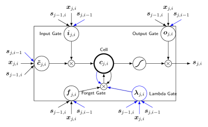
Figure 1: 2DLSTM unit. The additional links vs. standard LSTM are marked in blue.

The 2DLSTM has been introduced by Graves (2008) as a generalization of standard LSTM. Figure 1 illustrates one of the stable variants proposed by Leifert et al. (2016b). A 2DLSTM unit processes a 2D sequential data $x\in\mathbb{R}^{J\times I}$ of arbitrary lengths, $J$ and $I$. At time step $(j,i)$, the computation of its cell depends on both vertical ${s}_{j,i-1}$ and horizontal hidden states ${s}_{j-1,i}$ (see Equations 1–5). Similar to the LSTM cell, it maintains some state information in an internal cell state ${c}_{j,i}$. Besides the input ${i}_{j,i}$, the forget ${f}_{j,i}$ and the output ${o}_{j,i}$ gates that all control information flows, 2DLSTM employs an extra lambda gate ${\lambda}_{j,i}$. As written in Equ. 5, its activation is computed analogously to the other gates. The lambda gate is used to weight the two predecessor cells ${c}_{j-1,i}$ and ${c}_{j,i-1}$ before passing them through the forget gate (Equation 3). $g$ and $\sigma$ are the $\tanh$ and the sigmoid functions. $V$s, $W$s and $U$s are the weight matrices.

In order to train a 2DLSTM unit, back-propagation through time (BPTT) is performed over two dimensions Graves (2008, 2012). Thus, the gradient is passed backwards from the time step $(J,I)$ to $(1,1)$, the origin. More details, as well as the derivations of the gradients, can be found in Graves (2008).

$${i}_{j,i} =\sigma\Big{(}W_{1}{x}_{j,i}+U_{1}{s}_{j-1,i}+V_{1}{s}_{j,i-1}\Big{)}$$ (1)

$${f}_{j,i} =\sigma\Big{(}W_{2}{x}_{j,i}+U_{2}{s}_{j-1,i}+V_{2}{s}_{j,i-1}\Big{)}$$ (2)

$${o}_{j,i} =\sigma\Big{(}W_{3}{x}_{j,i}+U_{3}{s}_{j-1,i}+V_{3}{s}_{j,i-1}\Big{)}$$ (3)

$${\tilde{c}}_{j,i} =g\Big{(}W_{4}{x}_{j,i}+U_{4}{s}_{j-1,i}+V_{4}{s}_{j,i-1}\Big{)}$$ (4)

$${\lambda}_{j,i} =\sigma\Big{(}W_{5}{x}_{j,i}+U_{5}{s}_{j-1,i}+V_{5}{s}_{j,i-1}\Big{)}$$ (5)

$${c}_{j,i} ={f}_{j,i}\circ\big{[}{\lambda}_{j,i}\circ{c}_{j-1,i}+(1-{\lambda}_{j,i})\circ{c}_{j,i-1}\big{]}$$

$$\phantom{==}+{\tilde{c}}_{j,i}\circ{i}_{j,i}$$ (6)

$${s}_{j,i} =g\left({c}_{j,i}\right)\circ{o}_{j,i}$$ (7)

4 Two-Dimensional Sequence to Sequence Model

We aim to apply a 2DLSTM to map the source and the target sequences into a 2D space as shown in Figure 2. We call this architecture, the two-dimensional sequence to sequence (2D-seq2seq) model.

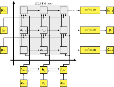
Figure 2: Two-dimensional sequence to sequence model (2D-seq2seq).

Given a source sequence $x_{1}^{J}=x_{1},\ldots,x_{J}$ and a target sequence $y_{1}^{I}=y_{1},\ldots,y_{I}$, we scan the source sequence from left to right and the target sequence from bottom to top as shown in Figure 2. In the 2D-seq2seq model, one dimension of the 2DLSTM (horizontal-axis in the figure) serves as the encoder and another (vertical axis) plays the role of the decoder. As a pre-step before the 2DLSTM, in order to have the whole source context, a bidirectional LSTM scans the input words once from left to right and once from right to left to compute a sequence of encoder states ${h}_{1}^{J}={h}_{1},\ldots,{h}_{J}$. At time step $(j,i)$, the 2DLSTM receives both encoder state, ${h}_{j}$, and the last target embedding vector, ${y}_{i-1}$, as an input. It repeatedly updates the source information, ${h}_{1}^{J}$, while generating new target word, ${y}_{i}$. The state of the 2DLSTM is computed as follows.

$${s}_{j,i}=\psi\Big{(}W\big{[}{h}_{j};{y}_{i-1}\big{]},U{s}_{j-1,i},V{s}_{j,i-1}\Big{)}$$ (8)

where $\psi$ stands for the 2DLSTM as a function. At each decoder step, once the whole source sequence is processed from $1$ to $J$, the last hidden state of the 2DLSTM, ${s}_{J,i}$, is used as the context vector. It means, at time step $i$, ${t}_{i}={s}_{J,i}$. In order to generate the next target word, ${y}_{i}$, a transformation followed by a softmax operation is applied. Therefore:

$$p_{i}(y_{i}=w|y_{1}^{i-1},x_{1}^{J})=\frac{\exp(W_{o}{t}_{iw})}{\sum_{v=1}^{|V_{t}|}\exp(W_{o}{t}_{iv})}$$ (9)

where $W_{o}$ and $|V_{t}|$ are the weight matrix and the target vocabulary respectively.

4.1 Training versus Decoding

One practical concern that should be noticed is the difference between the training and the decoding. Since the whole target sequence is known during training, all states of the 2DLSTM can be computed once at the beginning. Slices of it can then be used during the forward and backward training passes. In theory, the complexity of training is $\mathcal{O}(JI)$. But, in practice, the training computation can be optimally parallelized to take linear time Voigtlaender et al. (2016). During the decoding, only the already generated target words are available. Thus, either all 2DLSTM states have to be recomputed, or it has to be extended by an additional row at every time step $i$ that cause higher complexity.

Models Hidden Size De$\to$En En$\to$De devset newstest2016 newstest2017 devset newstest2016 newstest2017 Ppl Bleu Ter Bleu Ter Ppl Bleu Ter Bleu Ter 1 attention n=500 7.3 31.9 48.6 27.5 53.1 7.0 27.0 53.9 22.1 60.5 2 2D-seq2seq 6.5 32.6 47.8 28.2 52.7 6.1 27.5 53.8 22.4 60.6 3 + weighting 6.5 32.3 47.1 27.9 51.7 6.3 27.5 53.3 22.4 60.0 1 attention n=1000 6.4 33.1 47.5 29.0 51.9 6.5 27.4 53.9 22.9 60.2 2 2D-seq2seq 5.7 33.7 46.9 29.3 51.9 5.3 28.9 52.6 23.2 59.5 3 + weighting 6.1 32.7 47.1 28.0 51.9 5.7 27.8 53.0 22.7 60.0 4 coverage n=1000 6.3 33.1 47.5 28.7 51.9 5.8 28.6 52.4 23.0 59.4 5 fertility 6.2 33.4 46.9 28.9 51.6 5.8 28.4 52.1 23.2 59.1

Table 1: Bleu [%] and Ter [%] on the test sets and perplexity (Ppl) on the development set.

5 Experiments

We have done the experiments on the WMT 2017 German$\to$English and English$\to$German news tasks consisting of $4.6$M training samples collected from the well-known data sets Europarl-v7, News-Commentary-v10 and Common-Crawl. We use newstest2015 as our development set and newstest2016 and -2017 as our test sets, which contain $2169$, $2999$ and $3004$ sentences respectively. No synthetic data and no additional features are used. Our goal is to keep the baseline model simple and standard to compare methods rather that advancing the state-of-the-art systems.

After tokenization and true-casing using Moses toolkit Koehn et al. (2007), byte pair encoding (BPE) Sennrich et al. (2016) is used jointly with $20$k merge operations. We remove sentences longer than $50$ subwords and batch them together with a batch size of $50$. All models are trained from scratch by the Adam optimizer Kingma and Ba (2014), dropout of $30\%$ Srivastava et al. (2014) and the norm of the gradient is clipped with the threshold of $1$. The final models are the average of the $4$ best checkpoints of a single run based on the perplexity on the development set Junczys-Dowmunt et al. (2016). Decoding is performed using beam search of size $12$, without ensemble of various networks.

We have used our in-house implementation of the NMT system which relies on Theano Bastien et al. (2012) and Blocks Merriënboer et al. (2015). Our implementation of 2DLSTM is based on CUDA code adapted from Voigtlaender et al. (2016); Zeyer et al. (2018), leveraging some speedup.

The models are evaluated using case-sensitive Bleu Papineni et al. (2002) computed by mteval-v13a and case-sensitive Ter Snover et al. (2006) using tercom. We also report perplexities on the development set.

Attention Model: the attention based sequence to sequence model Bahdanau et al. (2014) is selected as our baseline that performs quite well. The model consists of one layer bidirectional encoder and a unidirectional decoder with an additive attention mechanism. All words are projected into a $500$-dimensional embedding on both sides. To explore the performance of the models with respect to hidden size, we try LSTMs Hochreiter and Schmidhuber (1997) with both $500$ and $1000$ nodes.

2D-Seq2Seq Model: we apply the same embedding size of that of the attention model. The 2DLSTM, as well as the bidirectional LSTM layer, are structured using the same number of nodes ($500$ or $1000$). The 2D-seq2seq model is trained with the learning rate of $0.0005$ vs. $0.001$ for the attention model.

Translation Performance: in the first set of experiments, we compare the 2D-seq2seq model with the attention sequence to sequence model. The results are shown in Table 1 in the rows $1$ and $2$. As it is seen, for size $n=500$, the 2D-seq2seq model outperforms the standard attention model on average by $0.7\%$ Bleu and $0.6\%$ Ter on De$\to$En, $0.4\%$ Bleu and no improvements in Ter on En$\to$De. The model is also superior for larger hidden size ($n=1000$) on average by $0.5\%$ Bleu and $0.3\%$ Ter on De$\to$En, $0.9\%$ Bleu and $1.0\%$ Ter on En$\to$De. In both cases, the perplexity of the 2D-seq2seq model is lower compared to that of the attention model.

The 2D-seq2seq topology is analogous to the bidirectional encoder-decoder model without attention. To examine whether the 2DLSTM reduces the need of attention, in the second set of experiments, we equip our model with a weighted sum of 2DLSTM states, ${t}_{i}$, over $j$ positions to dynamically select the most relevant information. In other words:

$$\gamma_{j,i} =\underset{j}{softmax}\Big{(}{v}^{T}\tanh\big{(}W{s}_{j,i}\big{)}\Big{)}$$ (10)

$${t}_{i} =\sum_{j=1}^{J}\gamma_{j,i}{s}_{j,i}$$ (11)

In these equations, $\gamma_{j,i}$ is the normalized weight over source positions, ${s}_{j,i}$ is the 2DLSTM states and $W$ and $v$ are weight matrices. As the results shown in the Table 1 in the rows $2$ and $3$, adding an additional weighting layer on top of the 2DLSTM layer does not help in terms of Bleu and rarely helps in Ter.

By updating the encoder states across the second dimension with respect to the target history, the 2D-seq2seq model can internally indicate which source words have already been translated and where it should focus next. Therefore, it reduces the risk of over- and under-translation. To examine our assumption, we compare the 2D-seq2seq model with two NMT models where the concepts such as fertility and coverage have been addressed Tu et al. (2016); Cohn et al. (2016).

source HP beschäftigte zum Ende des Geschäftsjahres 2013/14 noch rund 302.000 Mitarbeiter. reference At the end of the 2013/14 business year HP still employed around 302,000 staff. attention At the end of the financial year, HP employed some 302,000 employees at the end of the financial year of 2013/14. 2D-seq2seq HP still employs about 302,000 people at the end of the financial year 2013/14. coverage HP employed around 302,000 employees at the end of the fiscal year 2013/14. fertility HP employed some 302,000 people at the end of the fiscal year 2013/14.

Table 2: An example of over-translation.

Coverage Model: in the coverage model, we feed back the last alignments from the time step $i-1$ to compute the attention weight at time step $i$. Therefore, in the coverage model, we redefine the attention weight, $\alpha_{i,j}$, as:

$$\alpha_{i,j}=a\big{(}s_{i-1},h_{j},{\alpha}_{i-1,j}\big{)}$$ (12)

where $a$ is an attention function followed by the softmax. $h_{j}$ and $s_{i-1}$ are the the encoder and the previous decoder states respectively. In our experiments, we use additive attention similar to Bahdanau et al. (2014).

Fertility Model: in the fertility model, we feed back the sum of the alignments over the past decoder steps to indicate how much attention has been given to the source position $j$ up to step $i$ and divide it over the fertility of source word at position $j$. This term depends on the encoder states and it varies if the word is used in a different context Tu et al. (2016).

$$\beta_{i,j}=\frac{1}{N\cdot\sigma({\upsilon}^{\top}_{\phi}\cdot{h_{j}})}\sum_{k=1}^{i-1}\alpha_{i,j}$$ (13)

$$\alpha_{i,j}=a\big{(}s_{i-1},h_{j},{\beta}_{i,j}\big{)}$$ (14)

where $N$ specifies the maximum value for the fertility which set to 2 in our experiments. $\upsilon_{\phi}$ is a weight vector.

As it is seen in Table 1, rows $2$, $4$ and $5$, our proposed model is $0.3\%$ Bleu ahead and $0.3\%$ Ter worse compared to the fertility approach and slightly better compared to the coverage one. We note, the fertility and coverage models were trained using embedding size of $620$.

We have also qualitatively verified the coverage issue in Table 2 by showing an example from the test set. Without the knowledge of which source words have already been translated, the attention layer is at risk of attending to the same positions multiple times. This could lead to over-translation. Similarly, under-translation could be occur when the attention model rarely focusing at the corresponding source positions. As shown in the example, the 2DLSTM can internally track which source positions have already contributed to the target generation.

Speed: we have also compared the models in terms of speed on a single GPU training. In general, the training and decoding speed of the 2D-seq2seq model is $791$ and $0.7$ words/s respectively compared to those of standard attention model which is $2944$ and $48$ words/s. The computation of the added weighting mechanism is negligible in this case. This is still an initial architecture which indicates the necessity of multi-GPU usage. We also expect to speedup the decoding phase by avoiding the unnecessary recomputation of previous 2DLSTM states. In the current implementation, at each target step, we re-compute the 2DLSTM states from time step $0$ to $i-1$, while we only need to store the states from the last step $i-1$. This does not influence our results, as it is purely an implementation issue, not algorithm. However, decoding will still be slower than the training. One suggestion for further speedup of training phase is applying truncated BPTT on both directions to reduce the number of updates.

The 2DLSTM can be simply combined with self-attention layers Vaswani et al. (2017) in the encoder and the decoder for better context representation as well as RNMT+ Chen et al. (2018) that is composed of standard LSTMs. We believe that 2D-seq2seq model can be potentially applied to the other applications where sequence to sequence modeling is helpful.

6 Conclusion and Future Works

We have introduced a novel 2D sequence to sequence model (2D-seq2seq), a network that applies a 2DLSTM unit to read both the source and the target sentences jointly. Hence, in each decoding step, the network implicitly updates the source representation conditioned on the generated target words so far. The experimental results show that we outperform the attention model on two WMT 2017 translation tasks. We have also shown that our model implicitly handles the coverage issue.

As future work, we aim to develop a bidirectional 2DLSTM and consider stacking up 2DLSTMs for a deeper model. We consider the results promising and try more language pairs and fine-tune the hyperparameters.

References

- Bahdanau et al. (2014) Dzmitry Bahdanau, Kyunghyun Cho, and Yoshua Bengio. 2014. Neural machine translation by jointly learning to align and translate. CoRR, abs/1409.0473.
- Bastien et al. (2012) Frédéric Bastien, Pascal Lamblin, Razvan Pascanu, James Bergstra, Ian J. Goodfellow, Arnaud Bergeron, Nicolas Bouchard, and Yoshua Bengio. 2012. Theano: new features and speed improvements. Deep Learning and Unsupervised Feature Learning NIPS 2012 Workshop.
- Chen et al. (2018) Mia Xu Chen, Orhan Firat, Ankur Bapna, Melvin Johnson, Wolfgang Macherey, George Foster, Llion Jones, Niki Parmar, Mike Schuster, Zhifeng Chen, Yonghui Wu, and Macduff Hughes. 2018. The best of both worlds: Combining recent advances in neural machine translation. CoRR, abs/1804.09849.
- Cohn et al. (2016) Trevor Cohn, Cong Duy Vu Hoang, Ekaterina Vymolova, Kaisheng Yao, Chris Dyer, and Gholamreza Haffari. 2016. Incorporating structural alignment biases into an attentional neural translation model. In NAACL HLT 2016, The 2016 Conference of the North American Chapter of the Association for Computational Linguistics: Human Language Technologies, San Diego California, USA, June 12-17, 2016, pages 876–885.
- Gehring et al. (2017) Jonas Gehring, Michael Auli, David Grangier, Denis Yarats, and Yann N. Dauphin. 2017. Convolutional sequence to sequence learning. In Proceedings of the 34th International Conference on Machine Learning, ICML 2017, Sydney, NSW, Australia, 6-11 August 2017, pages 1243–1252.
- Graves (2008) Alex Graves. 2008. Supervised sequence labelling with recurrent neural networks. Ph.D. thesis, Technical University Munich.
- Graves (2012) Alex Graves. 2012. Supervised Sequence Labelling with Recurrent Neural Networks, volume 385 of Studies in Computational Intelligence. Springer.
- Graves and Schmidhuber (2008) Alex Graves and Jürgen Schmidhuber. 2008. Offline handwriting recognition with multidimensional recurrent neural networks. In Advances in Neural Information Processing Systems 21, Proceedings of the Twenty-Second Annual Conference on Neural Information Processing Systems, Vancouver, British Columbia, Canada, December 8-11, 2008, pages 545–552.
- Hochreiter and Schmidhuber (1997) Sepp Hochreiter and Jürgen Schmidhuber. 1997. Long short-term memory. Neural Computation, 9(8):1735–1780.
- Junczys-Dowmunt et al. (2016) Marcin Junczys-Dowmunt, Tomasz Dwojak, and Rico Sennrich. 2016. The AMU-UEDIN submission to the WMT16 news translation task: Attention-based NMT models as feature functions in phrase-based SMT. In Proceedings of the First Conference on Machine Translation, WMT 2016, Germany, pages 319–325.
- Kalchbrenner et al. (2015) Nal Kalchbrenner, Ivo Danihelka, and Alex Graves. 2015. Grid long short-term memory. CoRR, abs/1507.01526.
- Kingma and Ba (2014) Diederik P. Kingma and Jimmy Ba. 2014. Adam: A method for stochastic optimization. CoRR, abs/1412.6980.
- Koehn et al. (2007) Philipp Koehn, Hieu Hoang, Alexandra Birch, Chris Callison-Burch, Marcello Federico, Nicola Bertoldi, Brooke Cowan, Wade Shen, Christine Moran, Richard Zens, Chris Dyer, Ondrej Bojar, Alexandra Constantin, and Evan Herbst. 2007. Moses: Open source toolkit for statistical machine translation. In ACL 2007, Proceedings of the 45th Annual Meeting of the Association for Computational Linguistics, June 23-30, 2007, Prague, Czech Republic.
- Leifert et al. (2016a) Gundram Leifert, Tobias Strauß, Tobias Grüning, and Roger Labahn. 2016a. Citlab ARGUS for historical handwritten documents. CoRR, abs/1605.08412.
- Leifert et al. (2016b) Gundram Leifert, Tobias Strauß, Tobias Grüning, Welf Wustlich, and Roger Labahn. 2016b. Cells in multidimensional recurrent neural networks. The Journal of Machine Learning Research, 17(1):3313–3349.
- Li et al. (2017) Bo Li, Carolina Parada, Gabor Simko, Shuo yiin Chang, and Tara Sainath. 2017. Endpoint detection using grid long short-term memory networks for streaming speech recognition. In In Proc. Interspeech 2017.
- Li et al. (2016) Jinyu Li, Abdelrahman Mohamed, Geoffrey Zweig, and Yifan Gong. 2016. Exploring multidimensional lstms for large vocabulary ASR. In 2016 IEEE International Conference on Acoustics, Speech and Signal Processing, ICASSP 2016, Shanghai, China, March 20-25, 2016, pages 4940–4944.
- Merriënboer et al. (2015) Bart Merriënboer, Dzmitry Bahdanau, Vincent Dumoulin, Dmitriy Serdyuk, David Warde-Farley, Jan Chorowski, and Yoshua Bengio. 2015. Blocks and fuel: Frameworks for deep learning.
- Papineni et al. (2002) Kishore Papineni, Salim Roukos, Todd Ward, and Wei-Jing Zhu. 2002. Bleu: a Method for Automatic Evaluation of Machine Translation. In Proceedings of the 41st Annual Meeting of the Association for Computational Linguistics, pages 311–318, Philadelphia, Pennsylvania, USA.
- Sainath and Li (2016) Tara N. Sainath and Bo Li. 2016. Modeling time-frequency patterns with LSTM vs. convolutional architectures for LVCSR tasks. In Interspeech 2016, 17th Annual Conference of the International Speech Communication Association, San Francisco, CA, USA, September 8-12, 2016, pages 813–817.
- Sennrich et al. (2016) Rico Sennrich, Barry Haddow, and Alexandra Birch. 2016. Neural machine translation of rare words with subword units. In Proceedings of the 54th Annual Meeting of the Association for Computational Linguistics, ACL 2016, August 7-12, 2016, Berlin, Germany, Volume 1: Long Papers.
- Snover et al. (2006) Matthew Snover, Bonnie Dorr, Richard Schwartz, Linnea Micciulla, and John Makhoul. 2006. A Study of Translation Edit Rate with Targeted Human Annotation. In Proceedings of the 7th Conference of the Association for Machine Translation in the Americas, pages 223–231, Cambridge, Massachusetts, USA.
- Srivastava et al. (2014) Nitish Srivastava, Geoffrey E. Hinton, Alex Krizhevsky, Ilya Sutskever, and Ruslan Salakhutdinov. 2014. Dropout: a simple way to prevent neural networks from overfitting. Journal of Machine Learning Research, 15(1):1929–1958.
- Tu et al. (2016) Zhaopeng Tu, Zhengdong Lu, Yang Liu, Xiaohua Liu, and Hang Li. 2016. Modeling coverage for neural machine translation. In Proceedings of the 54th Annual Meeting of the Association for Computational Linguistics, ACL 2016, August 7-12, 2016, Berlin, Germany, Volume 1: Long Papers.
- Vaswani et al. (2017) Ashish Vaswani, Noam Shazeer, Niki Parmar, Jakob Uszkoreit, Llion Jones, Aidan N. Gomez, Lukasz Kaiser, and Illia Polosukhin. 2017. Attention is all you need. In Advances in Neural Information Processing Systems 30: Annual Conference on Neural Information Processing Systems 2017, 4-9 December 2017, Long Beach, CA, USA, pages 6000–6010.
- Voigtlaender et al. (2016) Paul Voigtlaender, Patrick Doetsch, and Hermann Ney. 2016. Handwriting recognition with large multidimensional long short-term memory recurrent neural networks. In 15th International Conference on Frontiers in Handwriting Recognition, ICFHR 2016, Shenzhen, China, October 23-26, 2016, pages 228–233.
- Wu et al. (2016) Yonghui Wu, Mike Schuster, Zhifeng Chen, Quoc V. Le, Mohammad Norouzi, Wolfgang Macherey, Maxim Krikun, Yuan Cao, Qin Gao, Klaus Macherey, Jeff Klingner, Apurva Shah, Melvin Johnson, Xiaobing Liu, Lukasz Kaiser, Stephan Gouws, Yoshikiyo Kato, Taku Kudo, Hideto Kazawa, Keith Stevens, George Kurian, Nishant Patil, Wei Wang, Cliff Young, Jason Smith, Jason Riesa, Alex Rudnick, Oriol Vinyals, Greg Corrado, Macduff Hughes, and Jeffrey Dean. 2016. Google’s neural machine translation system: Bridging the gap between human and machine translation. CoRR, abs/1609.08144.
- Zeyer et al. (2018) Albert Zeyer, Tamer Alkhouli, and Hermann Ney. 2018. RETURNN as a generic flexible neural toolkit with application to translation and speech recognition. In Proceedings of ACL 2018, Melbourne, Australia, July 15-20, 2018, System Demonstrations, pages 128–133.