Positional Cartesian Genetic Programming

Abstract

Cartesian Genetic Programming (CGP) has many modifications across a variety of implementations, such as recursive connections and node weights. Alternative genetic operators have also been proposed for CGP, but have not been fully studied. In this work, we present a new form of genetic programming based on a floating point representation. In this new form of CGP, called Positional CGP, node positions are evolved. This allows for the evaluation of many different genetic operators while allowing for previous CGP improvements like recurrency. Using nine benchmark problems from three different classes, we evaluate the optimal parameters for CGP and PCGP, including novel genetic operators.

1 Introduction

Cartesian Genetic Programming (CGP) is a form of Genetic Programming (GP) where program components are represented as functional nodes in on two dimensional grid. [Miller, 2011] Connections between these nodes are made based on their Cartesian coordinates and create a final computational structure. The node coordinates, the function of each node, and occasionally function parameters or node weights are encoded in a genome which is evolved using a $1+\lambda$ EA.

Originally created for circuit design, CGP has since been shown to have impressive results in image processing [Harding et al., 2013], creating neural networks [Khan et al., 2011] [Miller and Wilson, 2017], and playing video games [Wilson et al., 2018]. It can create understandable computational structures which illuminate solutions to the computational problems used as evolutionary fitness metrics. For example, in [Wilson et al., 2018], simple programs with constant or oscillatory behavior were generated by CGP, demonstrating effective strategies for certain video games. Despite their simplicity, many were competitive with or better than state of the art artificial agents.

CGP is an instance of graph-based GP, an attractive representation for computational structures given that they can reuse subgraph components and are used in many areas of computer science and engineering. In this work, we use ideas from other forms of graph-based GP to design new mutation and crossover methods for CGP. We also examine improvements to CGP that have been proposed, evaluating them as hyper-parameters and using a parameter search to determine when they are effective. These genetic operators and CGP enhancements are all evaluated as hyper-parameters on nine different benchmark problems, with three problems from each of the domains of classification, regression, and reinforcement learning.

Some of the new genetic operators are made possible by using a floating point representation of the CGP genome, as is done in [Clegg et al., 2007], with the addition of ’snapping’ connections which form connections to their nearest target node. Beyond enabling certain genetic operators, this representation allows for the evolution of the node positions itself, adding a new dimension to the CGP evolution. We term this representation Positional Cartesian Genetic Programming (PCGP) and evaluate it using the same hyper-parameter search used to evaluate CGP.

2 Cartesian Genetic Programming

In its original formulation, CGP nodes are arranged in a rectangular grid of $R$ rows and $C$ columns [Miller and Thomson, 2000]. Nodes are allowed to connect to any node from previous columns based on a connectivity parameter $L$ which sets the number of columns back a node can connect to; for example, if $L=1$, nodes could connect to the previous column only. In this paper, as in others, $R=1$, meaning that all nodes are arranged in a single row.

In this work, a floating point representation of CGP is used. A similar representation was previously used in [Clegg et al., 2007], but involved translation from the traditional integer CGP representation to floating point. Here, floats are used throughout. All genes are floating point numbers in $[0.0,1.0]$, which correspond to the connections of each node $n$, $x_{n}$ and $y_{n}$, the node function $f_{n}$, and a parameter gene $c_{n}$ which can be used for node weights or as a part of the function. Nodes are evenly spaced in one dimension between 0 and 1, with equal space around each node. Connections are formed by converting the connection genes $x_{n}$ and $y_{n}$ to coordinates by multiplying the genes by the node position, and then “snapping” these branches to the nearest node. An example of this process is shown in Figure 1.

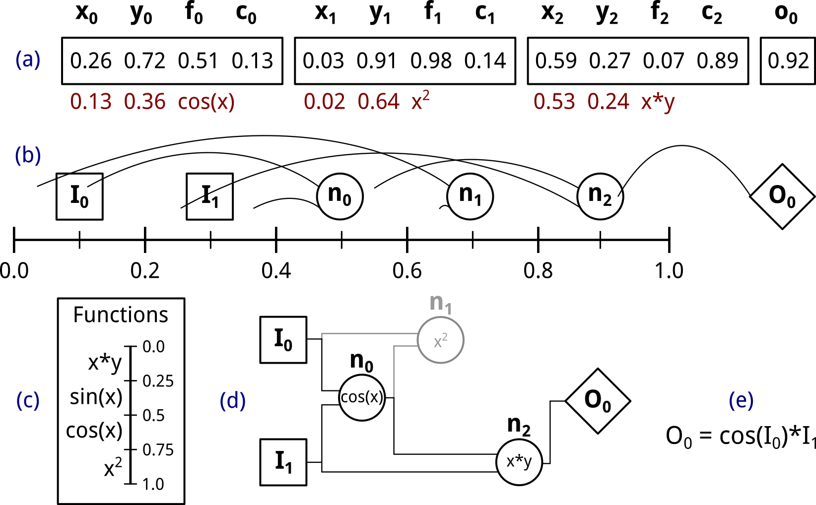
Figure 1: Translation of a floating point CGP genome into a program. The genome (a) is converted into positions and functions. The positions are informed by multiplying the connection genes, $x_{n}$ and $y_{n}$, by the position of the nodes, shown in (b). The functions are found by indexing the function gene $f_{n}$ in the Functions table (c). The resultant graph (d) is formed by “snapping” each connection to the closest node. As no output path uses $n_{1}$, this node is inactive or “junk”. Finally, the graph can be read as a simple program (e).

Each program output has a corresponding gene which connects to a node in the graph. The output gene $o_{n}$ specifies a connection which then “snaps” to the nearest node. By following connections back from the program outputs, an output program graph can be constructed. In practice, only a small portion of the nodes described by a CGP chromosome will be connected to its output program graph. These nodes which are used are called “active” nodes here, whereas nodes that are not connected to the output program graph are referred to as “inactive” or “junk” nodes. While these nodes do not actively contribute to the program’s output, they have been shown to aid evolutionary search [Miller and Smith, 2006], [Vassilev and Miller, 2000], [Yu and Miller, 2001].

Two established CGP modifications are explored in this work: recurrent CGP and node weights. In recurrent CGP [Turner and Miller, 2014] (RCGP), a recurrency parameter was introduced to express the likelihood of creating a recurrent connection; when $r=0$, standard CGP connections were maintained, but $r$ could be increased by the user to create recurrent programs. This work uses a slight modification of the meaning of $r$, but the idea remains the same. Here, the final connection position is modified by r:

$$p_{x_{n}}=x_{n}(r(1.0-p_{n})+p_{n})$$ (1)

where $p_{n}$ is the position of node $n$, $x_{n}$ is its connection gene, and $p_{x_{n}}$ is the position of the final connection. When $r=0.0$, this is as in standard floating point CGP, as presented in Figure 1, where $p_{x_{n}}=x_{n}p_{n}$. when $r=1.0$, the connection positions are simply the gene values, $p_{x_{n}}=x_{n}$. An example of this is shown in Figure 2. $r$ in this work therefore indicates the end of the possible range of connections for a node, from that node’s position $p_{n}$ to the end of the positional space, 1.0.

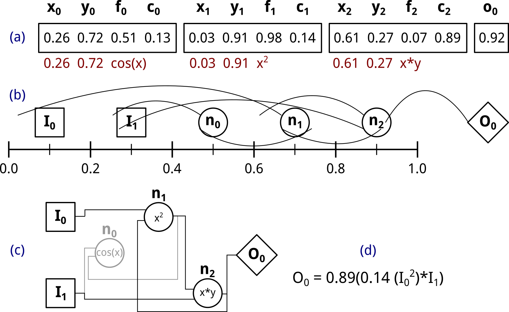
Figure 2: The same genome (a) as in Figure 1, but using a recurrency of $r=1.0$ and node weights $w=1$. The recurrency parameter changes the connection position calculation and allows nodes to connect to downstream nodes on their right (b). The output program graph (c) can then have recursive connections. Here, node weights are also used, modifying the final program (d).

In Figure 2, node weights are also used. In this scheme, the output of each node is multiplied by its parameter gene $c_{n}$. This CGP modification has allowed for differentiable CGP [Izzo et al., 2017] and is referred to in this work by the binary hyper-parameter $w$, which is true ($w=1$) when weights are used.

3 Positional Cartesian Genetic Programming

With floating point CGP as a base, Positional CGP introduces a small modification which allows for many possibilities. Each node also has a position gene, $p_{n}$, which determines the position of the node, instead of spacing each node equally between 0.0 and 1.0. In CGP, a connection has equal probability of connecting to each node previous to its parent. In PCGP, this probability is evolved based on the positions of each node.

Evolving the node positions complicates the role of the inputs, however. In SM-CGP, where it also isn’t certain the graph will include inputs, program input is a function which nodes can choose [Harding et al., 2010]. In this work, we chose to place input in an evolved space to the left of the linear node space, ensuring that nodes form connections to inputs while allowing the inputs to also form their own connection distributions through evolution. Each inputs has a positional gene, $i_{n}$, which is multiplied by a hyper-parameter which determines the start of the input space, $I_{start}$. This input position gene is initialized like all other genes, randomly in a uniform distribution in [0.0, 1.0]. Node position calculation is modified with $I_{start}$ to contain the entire space, including the input space:

$$p_{x_{n}}=x_{n}((r(1.0-p_{n})+p_{n})-I_{start})+I_{start}$$ (2)

When $I_{start}=-1.0$, as in Figure 3, the input space is large and nodes have a high probability of connecting directly to inputs. As this is not desirable for complex programs, the $I_{start}$ parameter was tested in the following experiments.

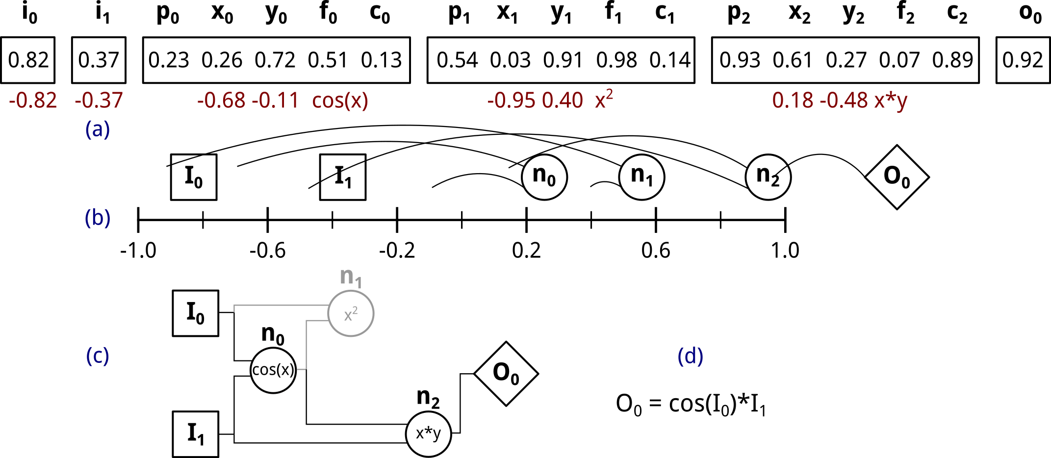
Figure 3: A PCGP genome (a), including input $i_{n}$ and positional $p_{n}$ genes. These are translated to input and node positions (b) and connection positions “snap” to the nearest node, as in floating point CGP. As in CGP, a resultant graph (c) and output program (d) are then extracted.

Due to the evolution of the positions, it is highly likely that no two nodes occupy the same position, even between different genomes. Furthermore, over evolution, nodes which are connected can have positional genes and connection genes which are highly related. Finally, a node’s connection positions depend only on that node’s position, which is in its genes, and not on the node’s placement in the genome or other nodes in the network. This allows node genes to be exportable; the same genes in a different individual will form connections in the same place. If multiple genes are exported together, entire sections of the graph can be migrated between individuals. In PCGP, nodes can be added or removed from a genome without disturbing the existing connection scheme, unlike in CGP, where a node addition and deletion causes a shift in all downstream node positions. This is the inspiration for the following study, where graph based operators from other forms of GP are used in PCGP.

4 Genetic operators

GP has numerous genetic operators defined across its many implementations. Genetic mutation and single point crossover have been used extensively, but tree-based GP also mutates and crosses specific parts of a genome. Autoconstructive evolution introduced many operators as part of a program modification instruction set [Spector, 2002]. Evolution of artificial neural networks (ANN) [Stanley and Miikkulainen, 2002] and gene regulatory networks (GRN) [Cussat-Blanc et al., 2015] provide examples of genetic operators especially suited for genomes that encode graphs, which is relevant to both CGP and PCGP. Parallel distributed GP (PDGP) was inspired by ANNs and included a subgraph addition mutation and a subgraph crossover method called subgraph active-active node (SAAN) [Poli et al., 1997]. A comparison of different crossover operators and ideal parameters for these methods is presented in [Husa and Kalkreuth, 2018]. Here we define multiple genetic operators for both CGP and PCGP drawn from other GP methods, ANN evolution, and GRN evolution. Operators are defined in bold and common methods used by multiple operators are defined in italics.

4.1 Mutation

First, we define common methods used by multiple operators. We use the term “computational nodes” to refer to CGP or PCGP nodes which are neither inputs nor outputs.

Node addition: $m_{\delta}size_{min}$ computational nodes with random genes are added to the end of the genome. In PCGP, these are then sorted into the genome based on position.

Node deletion: $m_{\delta}size_{min}$ computational nodes are randomly selected from the genome and removed. In the event that there are fewer than $m_{\delta}size_{min}$ computational nodes, all computational nodes are removed.

Subgraph addition: $m_{\delta}size_{min}$ computational nodes are added to the genome. The position, function, and parameter genes are randomly chosen, but connection genes are selected randomly out from a pool. For each new node $i$, this pool composed of all other new nodes with position $p<p_{i}$. An equal number of randomly selected computational and input nodes with $p<p_{i}$ are also added to the pool from the parent chromosome. By fixing the connection genes, the new genetic material is guaranteed to either contain new subgraphs or to create a subgraph with existing nodes. Due to the requirement of knowing exact node positions for connection, this operation is available only in PCGP.

Subgraph deletion: The parent genome is evaluated into functional trees, both those which result in a final output (active) and those which don’t (inactive or junk). A tree with more than 1 computational node is chosen randomly and up to $m_{delta}size{min}$ computational nodes are removed from it.

These methods are used in the following three mutation operators:

(1) Gene mutation: In CGP and PCGP, each gene of the computational nodes has a $m_{node}$ chance of being replace by a new random value in $[0.0,1.0]$. Outputs are similarly mutated with a $m_{output}$ chance. In PCGP only, the positions of the inputs are mutated with a $m_{input}$ chance. If $m_{active}$ is true, this mutation is repeated until a gene in an active node is mutated [Goldman and Punch, 2013].

(2) Mixed node mutate: A random method between gene mutation, node addition, and node deletion is chosen according to $m_{modify}$ and the size of the parent genome. A random number $r$ is chosen in $[0.0,1.0]$. If $r$ is less than $m_{modify}$, gene mutation is selected. If $r$ is less than $m_{modify}+m_{add}$, node addition is selected. Otherwise, node deletion is selected. $m_{add}$ is calculated based on the number of nodes in the parent genome, $n$:

$$m_{add}=\frac{(n-size_{min})(1-m_{modify})}{size_{max}-size_{min}}$$

(3) Mixed subgraph mutate: Following the same logic as mixed node mutate, a method between gene mutation, subgraph addition, and subgraph deletion is chosen according to $m_{modify}$ and the size of the parent genome.

4.2 Crossover

For CGP, three crossover methods have been defined: single point, random node, and proportional. As PCGP allows for program structure to be preserved during genetic transfer and contains additional genetic material in the form of positions, further crossover methods can be defined: aligned node, output graph, and subgraph.

(1) Single point crossover: In this classic crossover operator, a single point in the two parent genomes is selected randomly. The genetic material before this point is taken randomly from one parent and the genetic material after this points is taken from the other parent. In CGP and PCGP, the point is constrained to the beginning of a node’s genetic material.

(2) Random node crossover: Nodes are randomly selected equally from both parents. A child is constructed using randomly selected input and output genes from both parents, the selected computational node genes from the first parent, then finally the selected computational node genes from the second parent. The ordering of the genetic material is important for CGP, but in PCGP the nodes and their corresponding genes are ordered by their position.

(3) Aligned node crossover: This operator is only applicable for PCGP. Nodes are first paired from each parent based on position proximity, This operator then follows the same method as random node crossover, however nodes are randomly chosen from their position aligned pairs.

(4) Proportional crossover: This operator was previously explored in [Clegg et al., 2007]. The child’s genetic material $C$, up to the minimum size of both parents ($A$ and $B$), is combined using a vector of randomly chosen weights, $w$:

$$C_{i}=(1-w_{i})A_{i}+w_{i}B_{i}\leavevmode\nobreak\ \leavevmode\nobreak\ \forall i$$ (3)

If one parent genome was longer than the other, the remaining genetic material is appended to the end of the child genome.

(5) Output graph crossover: Outputs from each parent are randomly selected for the child genome. For each selected output, the full functional graph resulting in this output is computed, and the set of all computational nodes in the selected output graphs for each parent is used to construct the child genome. Functional arity is ignored in this output trace, meaning that inactive genetic material from 1-arity functions will be passed on to the child genome. Otherwise, this operator only takes active nodes from each parent. If an input is used in only one parent’s selected output graph, it is passed on to the child directly. Otherwise, each input is randomly selected from both parents. As this operator assumes that the functional graph directly corresponds to the transferred genetic material, it is only available in PCGP.

(6) Subgraph crossover: Similarly to output graph crossover, the functional graphs from the parent genomes are computed. However, in this operator, active and inactive subgraphs from both parents are randomly selected equally. Input and output genes are selected randomly from both parents. As with output graph crossover, this operator is only applicable to PCGP.

5 Experiments

Parameter	type	range
mutation	c	genetic, mixed node, mixed subgraph
crossover	c	single point, proportional, random node, aligned node, output graph, subgraph
$\lambda$ (population)	i	[1, 10]
GA population	c	20, 40, 60, 80, 100, 120, 140, 160, 200
$I_{start}$	r	[-1.0, -0.1]
$r$	r	[0.0, 1.0]
$w$	c	true, false
$m_{active}$	c	true, false
$m_{input}$	r	[0.0, 1.0]
$m_{output}$	r	[0.1, 1.0]
$m_{node}$	r	[0.1, 1.0]
$m_{\delta}$	r	[0.1, 0.5]
$m_{modify}$	r	[0.1, 0.9]
$GA_{elitism}$	r	[0.0, 0.8]
$GA_{crossover}$	r	[0.1, 1.0]
$GA_{mutation}$	r	[0.1, 1.0]

Table 1: Ranges used in irace. The different range types are choice (c), integer (i), and real-valued (r). The precision for real-valued parameters was 0.1.

To explore the utility of these different genetic operators in CGP and PCGP, a parameter study is done using irace [López-ibáñez et al., 2016]. irace is an automatic algorithm configuration package which selects from ranges of parameters and explores the parameter space efficiently by focusing on high performing parameter sets in a method known as racing.

The different genetic operators are parameterized and included with all CGP and PCGP parameters for irace optimization. A $1+\lambda$ EA and a GA are used, and the necessary parameters for the two are also optimized. The GA includes the parameters $GA_{elitism}$, determining the number of top individuals retained each generation, $GA_{crossover}$, the percentage of new individuals produced by crossover, and $GA_{mutation}$, the percentage of individuals produced by mutation. If these three sum to less than 1.0, random tournament winners are added to the population unmodified. CGP and PCGP are evaluated separately, and each is evaluated on an EA and GA separately, creating four different parameter optimization cases.

These four cases are evaluated using nine benchmarks: three classification problems, three regression problems, and three reinforcement learning or control problems. The classification and regression problems are from the UCI machine learning repository . The classification problems are the breast cancer, diabetes, and glass datasets, which are standard problems in classification and represent different challenges in classification. The regression datasets are abalone, wine quality, and forest fire area, which are also standard benchmark sets. The reinforcement learning tasks are three locomotion tasks from the PyBullet library [Coumans and Bai, 2018]. In these tasks, a robotic ant, cheetah, and humanoid must be controlled to walk as far as possible from the starting point.

	$e_{0}$			$e_{1}$			$e_{2}$
	$1+\lambda$			$1+\lambda$			GA
	CGP			PCGP			CGP
class	C	R	RL	C	R	RL	C	R	RL
mutation	node	gene	gene	gene	node	node	gene	gene	gene
crossover							sp	sp	sp
population	4	9	4	6	3	8	20	120	200
$I_{start}$				-0.5	-0.5	-0.5
$r$	0.2	0.1	0.6	0.5	0.4	0.1	0.4	0.1	0.8
$w$	0	0	1	0	0	1	0	0	0
$m_{active}$	1	1	0	0	0	0	0	1	1
$m_{input}$				0.1	0	0.3
$m_{output}$	0.2	0.1	0.3	0.3	0.2	0.8	0.1	0.5	0.3
$m_{node}$	0.1	0.1	0.1	0.1	0.1	0.2	0.2	0.1	0.1
$m_{\delta}$	0.4				0.2	0.2
$m_{modify}$	0.6				0.9	0.5
$GA_{elitism}$							0.1	0.2	0.1
$GA_{crossover}$							0.2	0.2	0.2
$GA_{mutation}$							0.3	0.6	0.2
	$e_{3}$			$e_{4}$			$e_{5}$
	GA			$1+\lambda$			GA
	PCGP			CGP			CGP
class	C	R	RL	all			all
mutation	gene	gene	node		gene			gene
crossover	prop	prop	output					prop
population	120	80	200		5			50
$I_{start}$	-0.9	-0.2	-0.3
$r$	0.5	0.1	0.2		0.0			0.0
$w$	0	0	1		0			0
$m_{active}$	0	1	1		0			0
$m_{input}$	0	0	0.2
$m_{output}$	0.2	0.4	0.3		0.1			0.2
$m_{node}$	0.1	0.1	0.4		0.1			0.2
$m_{delta}$			0.3
$m_{modify}$			0.4
$GA_{elitism}$	0.2	0.4	0.4					0.04
$GA_{crossover}$	0.1	0.2	0.5					0.5
$GA_{mutation}$	0.7	0.4	0.1					1.0

Table 2: The optimized parameter sets, $e_{0}$ through $e_{3}$, found by irace, and the default parameter sets $e_{4}$ and $e_{5}$. The different problem types are classification (C), regression (R), and reinforcement learning (RL). The mutation methods used are genetic mutation (gene) and mixed node mutation (node). The crossover methods used are single point (sp), proportional (prop), and output graph (output).

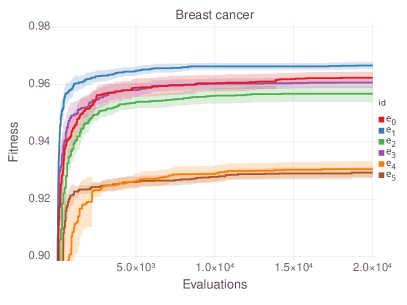
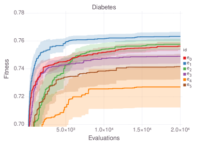
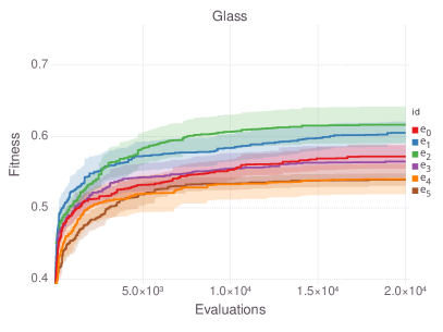
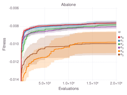
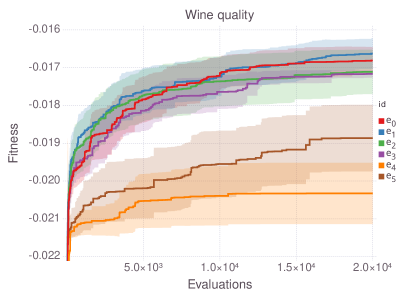
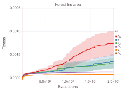
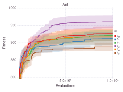
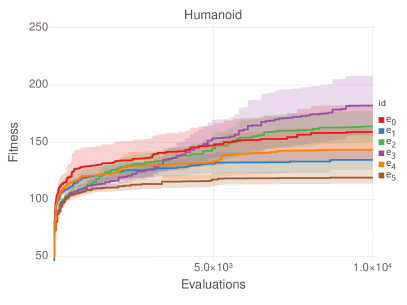
Figure 4: Comparison of the different methods on eight of the nine problems. Cheetah locomotion is omitted for space, due to similar results for all tested methods. Lines show the average of the best individuals and ribbons show one standard deviation from 20 trials.

6 Method comparison

First, we compare the four different methods, $1+\lambda$ EA and a GA, using both CGP and PCGP, using the best parameters found by irace for the set of three problems of each type. The optimized methods are compared to the default parameters of CGP, $e_{4}$ and the parameters reported in [Clegg et al., 2007], $e_{5}$, as it is a similar work which uses crossover and a floating point representation. The crossover rate was chosen based on the results from [Clegg et al., 2007], although that work includes an interesting study of a variable crossover rate, which was not implemented for these experiments. The optimized and default parameters are presented in Table 2.

These parameters were used in 20 evolutions on each of the nine problems. To compare the different population sizes and methods, the results are compared based on the number of fitness evaluations, not by generation. For the classification and regression problems, each evolution was run for 20000 evaluations and 10000 for the RL problems, as these problems were far more computationally expensive. The computational budget in terms of nodes was also considered; as some methods have a variable genome size, allowing them to increase their computational limit in a way static methods cannot, the variable methods were constrained to $[0.5,1.5]$ of the genome size for the static methods.

Overall, the results, displayed in Figure 4, show that the optimized parameter sets perform better than the two default parameter sets, $e_{4}$ and $e_{5}$. Between the four optimized methods, there is no clear winner. $e_{1}$, the $1+\lambda$ PCGP EA, is superior on two of the classification problems, but not on the other problems, especially RL, where it is the worst of the optimized methods. $e_{3}$, the PCGP GA, is superior on two of the RL problems, but performs badly on classification and regression.

It is worth noting that, while the GA methods $e_{2}$ and $e_{3}$ don’t always perform the best, their results are competitive with the $1+\lambda$ EA methods. While this comparison is based on number of fitness evaluations, the GA has the advantage of massive parallelization that the EA doesn’t. In the GA, a generation of up to 200 individuals can be evaluated in parallel, giving similar results to the EA methods in a fraction of the time.

The main conclusion that can be drawn from this comparison is that the choice of method, and the parameters of the chosen method, can greatly improve CGP performance. To better understand appropriate parameters, therefore, we next analyze the full results from irace, beyond the best individual used in these comparisons.

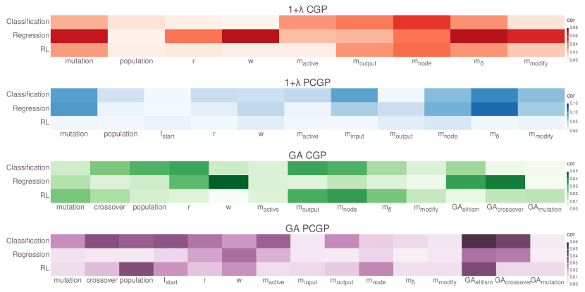
Figure 5: Correlation of all parameters with evolutionary fitness, using all parameter sets explored by irace. Each color represents a different method, and the color intensity represents the correlation with fitness for that parameter. Correlations are divided by problem class (classification, regression, and RL), using the final fitness results from all problems in the specific class

.

7 Parameter study

Finally, we explore the parameter choices produced by irace. The top 20 parameters, called expert parameter sets, for each method are displayed for the different class types in Figure 6 and Figure 7, and the correlation between each parameter and evolutionary fitness is shown in Figure 5. In Figure 6 and Figure 7, all parameters are represented as values between 0.0 and 1.0. To achieve this, the mutation operators were ordered as [genetic, mixed node, mixed subtree], being [0.0, 0.5, 1.0], and the crossover operators were ordered [single point, proportional, random node, aligned node, output graph, subgraph], being [0.0, 0.2, 0.4, 0.6, 0.8, 1.0]. The population parameter represents $\frac{\lambda}{10}$ for the $1+\lambda$ EA and $\frac{population}{200}$ for the GA. Finally, $I_{start}$ is represented as $1+I_{start}$.

For CGP with the $1+\lambda$ EA, there is a clear preference for gene mutation over mixed node mutation across all problems. Mutation rates are important, and most expert parameters have a slightly higher output mutation rate than node mutation rate, with $m_{output}$ reaching as high as 0.5 in many experts. Node weights, $w$, especially have an impact for regression, where they should not be used. Active mutation, $m_{active}$, appears useful mostly for classification and regression and isn’t correlated with fitness for RL tasks. Finally, $\lambda$ appears to have little effect on the outcome, and $r$ appears to impact the result only in the case of regression tasks, when it should be low.

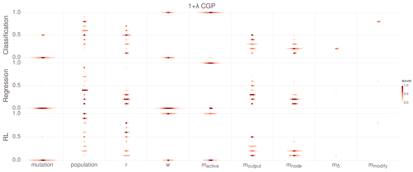
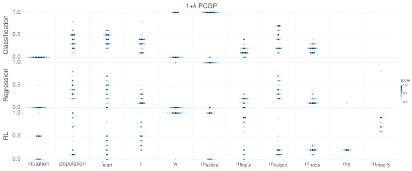
Figure 6: Parameters for the top 20 $1+\lambda$ EA configurations, for CGP and PCGP

The expert parameter results for PCGP with the $1+\lambda$ EA are similar to that with CGP. Gene mutation is a clear winner, using a higher mutation rate for outputs than inputs and nodes. $\lambda$, $I_{start}$, and $r$ aren’t strongly correlated with fitness. Node weights appear useful in RL problems but are detrimental in classification and regression problems, and active mutation appears generally useful. An interesting difference in $1+\lambda$ EA PCGP is the prevalence of mixed node mutation in expert parameter sets for RL problems. However, due to a high $m_{modify}$ of these parameter sets, the main functional mutation in these expert sets remained a gene modification mutation, with rare node addition and deletion events.

For CGP, the expert parameters for a GA are very similar to the $1+\lambda$ CGP EA expert parameters. Population is much more important than in the $1+\lambda$ EA, with medium to large populations (100 to 200 individuals) showing an advantage in classification and regression problems. Genetic mutation is the clear choice for a mutation operator, while crossover is split between single point for classification and proportional for regression and RL. Elitism is rather high, reaching 50% in some expert sets. Crossover rates are low, except in the case of classification, where it has little bearing on the final outcome.

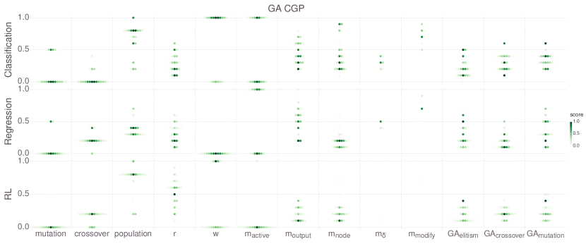
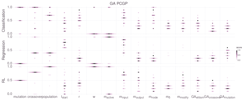
Figure 7: Parameters for the top 20 GA configurations, for CGP and PCGP.

The parameter results for PCGP when using a GA are very interesting and different from all other sets. Here, we see usage of the other mutation and crossover operators; classification prefers mixed subtree mutation and subgraph crossover, regression uses gene mutation and random node crossover, and RL uses mixed node mutation with output graph crossover. The population is somewhat problem dependent, but is especially important in RL, where large populations are favorable. Node weights are highly preferred in RL, but not in regression or classification. Elitism has a large impact on the final fitness, although the values for RL and classification are spread almost evenly between 0.1 and 0.5.

Considering the success of $e_{3}$ on the RL problems, the PCGP GA parameters show that output graph crossover and node-based mutation can be viable strategies for PCGP evolution. It’s notable also that subgraph crossover was used in expert regression sets and favored in classification, showing that graph-based operations can be useful generally. The RL problems have outputs corresponding to the control of different limbs, which may offer more modularity than the different classes of classification.

8 Conclusion

Positional CGP opens the possibility of doing graph operations during CGP evolution. The experiments in this work demonstrate that there is the potential for improvement of CGP’s evolution, even if no single method proposed is universally dominant. The possibilities in improving CGP evolution are expanded by PCGP, and more work is needed to explore these potential improvements.

Some of the parameters explored in this work are at the level of evolution and require global coordination. Others, such as $r$, $I_{start}$, $w$, etc, could be included at the level of the genome. Even the choice of CGP or PCGP could be a binary parameter within the genome, deciding if the positional genes are used or not. This would allow an individual optimization of the hyper-parameters and reduce the burden of parameter choice.

The global parameters could also benefit from dynamic change over evolution. In [Clegg et al., 2007], a variable crossover rate which begins high and reduces to 0 as the population converges is used. Adaptive mutation rates have also been proven to increase search for the $1+(\lambda,\lambda)$ EA [Doerr and Doerr, 2018] and could benefit CGP.

Other methods of evolution are also made possible by this work. CMA-ES could easily be used to evolve floating point CGP or PCGP. In [Harding et al., 2013], an island-based $1+\lambda$ EA is used. The graph-based crossover methods presented in this work might the integration of experts in that scheme. In [Zaefferer et al., 2018], multiple distance metrics for GP are evaluated. These could be used in CGP or PCGP to introduce speciation to the GA, achieving a similar effect to the island-based model.

Finally, this work offers a guide to CGP configuration, including parameters for a successful GA evolution, which has not been the standard for CGP. Given the quality of the results attained by CGP, the benefits of parallelism could be used to solve many problems to which GP has yet to be applied.

Acknowledgments

This work is supported by ANR-11-LABX-0040-CIMI, within programme ANR-11-IDEX-0002-02.

References

- [Clegg et al., 2007] Clegg, J., Walker, J. A., and Miller, J. F. (2007). A new crossover technique for Cartesian genetic programming. In Proceedings of the 9th annual conference on Genetic and evolutionary computation - GECCO ’07, page 1580, New York, New York, USA. ACM Press.
- [Coumans and Bai, 2018] Coumans, E. and Bai, Y. (2016–2018). Pybullet, a python module for physics simulation for games, robotics and machine learning. http://pybullet.org.
- [Cussat-Blanc et al., 2015] Cussat-Blanc, S., Harrington, K., and Pollack, J. (2015). Gene regulatory network evolution through augmenting topologies. IEEE Transactions on Evolutionary Computation, 19(6):823–837.
- [Doerr and Doerr, 2018] Doerr, B. and Doerr, C. (2018). Optimal static and self-adjusting parameter choices for the genetic algorithm. Algorithmica, 80(5):1658–1709.
- [Goldman and Punch, 2013] Goldman, B. W. and Punch, W. F. (2013). Reducing wasted evaluations in cartesian genetic programming. In European Conference on Genetic Programming, pages 61–72. Springer.
- [Harding et al., 2010] Harding, S., Banzhaf, W., and Miller, J. F. (2010). A Survey of Self Modifying Cartesian Genetic Programming. Genetic Programming Theory and Practice VIII, 8:91–107.
- [Harding et al., 2013] Harding, S., Leitner, J., and Schmidhuber, J. (2013). Cartesian genetic programming for image processing. In Genetic programming theory and practice X, pages 31–44. Springer.
- [Husa and Kalkreuth, 2018] Husa, J. and Kalkreuth, R. (2018). A comparative study on crossover in cartesian genetic programming. In European Conference on Genetic Programming, pages 203–219. Springer.
- [Izzo et al., 2017] Izzo, D., Biscani, F., and Mereta, A. (2017). Differentiable genetic programming. In European Conference on Genetic Programming, pages 35–51. Springer.
- [Khan et al., 2011] Khan, G. M., Miller, J. F., and Halliday, D. M. (2011). Evolution of cartesian genetic programs for development of learning neural architecture. Evolutionary computation, 19(3):469–523.
- [López-ibáñez et al., 2016] López-ibáñez, M., Dubois-lacoste, J., Pérez, L., Birattari, M., and Stützle, T. (2016). The irace package : Iterated racing for automatic algorithm configuration. 3:43–58.
- [Miller, 2011] Miller, J. F. (2011). Cartesian Genetic Programming. Natural Computing Series. Springer Berlin Heidelberg, Berlin, Heidelberg.
- [Miller and Smith, 2006] Miller, J. F. and Smith, S. L. (2006). Redundancy and computational efficiency in Cartesian Genetic Programming. IEEE Trans. on Evolutionary Computation, 10(2):167–174.
- [Miller and Thomson, 2000] Miller, J. F. and Thomson, P. (2000). Cartesian genetic programming. In Proc. European Conf. on Genetic Programming, volume 10802 of LNCS, pages 121–132.
- [Miller and Wilson, 2017] Miller, J. F. and Wilson, D. G. (2017). A developmental artificial neural network model for solving multiple problems. In Proceedings of the Genetic and Evolutionary Computation Conference Companion, pages 69–70. ACM.
- [Poli et al., 1997] Poli, R. et al. (1997). Evolution of graph-like programs with parallel distributed genetic programming. In ICGA, pages 346–353. Citeseer.
- [Spector, 2002] Spector, L. E. E. (2002). Genetic Programming and Autoconstructive Evolution with the Push Programming Language. pages 7–40.
- [Stanley and Miikkulainen, 2002] Stanley, K. O. and Miikkulainen, R. (2002). Evolving neural networks through augmenting topologies. Evolutionary computation, 10(2):99–127.
- [Turner and Miller, 2014] Turner, A. J. and Miller, J. F. (2014). Recurrent cartesian genetic programming. In Proc. Parallel Problem Solving from Nature, pages 476–486.
- [Vassilev and Miller, 2000] Vassilev, V. K. and Miller, J. F. (2000). The Advantages of Landscape Neutrality in Digital Circuit Evolution. In Proc. Int. Conf. on Evolvable Systems, volume 1801 of LNCS, pages 252–263. Springer Verlag.
- [Wilson et al., 2018] Wilson, D. G., Cussat-Blanc, S., Luga, H., and Miller, J. F. (2018). Evolving simple programs for playing atari games. In Proceedings of the Genetic and Evolutionary Computation Conference. ACM.
- [Yu and Miller, 2001] Yu, T. and Miller, J. F. (2001). Neutrality and the Evolvability of Boolean function landscape. In Proc. European Conference on Genetic Programming, volume 2038 of LNCS, pages 204–217.
- [Zaefferer et al., 2018] Zaefferer, M., Stork, J., Flasch, O., and Bartz-Beielstein, T. (2018). Linear combination of distance measures for surrogate models in genetic programming. In International Conference on Parallel Problem Solving from Nature, pages 220–231. Springer.