Distributions of Pseudo-Redshifts and Durations (Observed and Intrinsic) of Fermi GRBs

Abstract

Ever since the insightful analysis of the durations of gamma-ray bursts (GRBs) by Kouveliotou et al. (1993), GRBs have most often been classified into two populations: “short bursts" (shorter than 2.0 seconds) and “long bursts" (longer than 2.0 seconds). However, recent works have suggested the existence of an intermediate population in the bursts observed by the Swift satellite. Moreover, some researchers have questioned the universality of the 2.0-second dividing line between short and long bursts: some bursts may be short but actually result from collapsars, the physical mechanism behind normally long bursts, and some long ones may originate from mergers, the usual progenitors of short GRBs.

In this work, we focus on GRBs detected by the Fermi satellite (which has a much higher detection rate than Swift and other burst-detecting satellites) and study the distribution of their durations measured in the observer’s reference frame and, for those with known redshifts, in the bursts’ reference frames. However, there are relatively few bursts with measured redshifts, and this makes an accurate study difficult. To overcome this problem, we follow Zhang and Wang (2018) and determine a “pseudo-redshift" from the correlation relation between the luminosity $L_{p}$ and the energy $E_{p}$, both of which are calculated at the peak of the flux. Interestingly, we find that the uncertainties in the quantities observed and used in the determination of pseudo-redshifts, do affect the precision of the individual results significantly, but they keep the distribution of pseudo-redshifts very similar to that of the actual ones and thus allow us to use pseudo-redshifts for our statistical study. We briefly present the advantages and disadvantages of using pseudo-redshifts in this context.

We use the reduced chi-square and the maximization of the log-likelihood to statistically analyze the distribution of Fermi GRB durations. Both methods show that the distribution of the observed (measured) and the intrinsic (source/rest frame) bursts durations are better represented by two groups/populations, rather than three.

Keywords Gamma-rays: bursts, theory, observations; Methods: data Analysis, statistical, chi-square test, likelihood.

1 Introduction

Gamma-ray bursts (GRBs) are the most energetic electromagnetic events known in the cosmos. They have been studied in depth since their discovery in the late 1960’s (first reported by Klebesadel et al. (1973)). While the cosmological (extra-galactic) origin of the GRBs is well established (since it was confirmed by the spatially isotropic distribution of bursts detected by the CGRO/BATSE instrument in the 1990’s and from the redshift measurements, starting with Metzger et al. (1997)), questions about their sources and their physical nature remain incompletely resolved. It is, however, commonly assumed that GRBs result from different, heterogeneous populations and characteristics (see, most recently, Zhang et al. (2014); Shahmoradi and Nemiroff (2015); Chattopadhyay and Maitra (2017)).

Various descriptive and statistical studies have been conducted using GRB data obtained with instruments that work in several bands of the electromagnetic spectrum. The duration of a burst is one of the most commonly used parameters for classifying and characterizing gamma-ray bursts (from Kouveliotou et al. (1993) to Zitouni et al. (2015); Tarnopolski (2015a, 2016a, 2016b, 2016c); Kulkarni and Desai (2017); Zhang and Wang (2018)). Burst durations are most often defined by $T_{90}$, the time interval over which 90% of the total fluence (integrated flux, minus the background) is recorded (Kouveliotou et al., 1993; Koshut et al., 1995)

Most of the statistical studies on the distribution of $T_{90}$ durations are consistent with the existence of two populations of bursts, but a relatively small number of works have found in the data indications that a third, intermediate group might exist (Horváth (1998); Balastegui et al. (2001); Chattopadhyay et al. (2007); Horváth et al. (2008); Zitouni et al. (2015); Zhang et al. (2016); Kulkarni and Desai (2017)). The existence of two different populations is now fully confirmed: a consensus exists on the hypernova-collapsar nature of long bursts, and with the August 2017 observational confirmation of a merger of two neutron stars (via the detection of both gravitational waves and electromagnetic radiation from a short GRB, GW/GRB170817 – Abbott et al. (2017a, b)), the merger nature of short bursts appears to now be firmly established. Still, a third (intermediate) population is not totally rejected.

In this work, we wish to explore the distribution of Fermi GRB durations, using the data published on its website (von Kienlin et al., 2014; Narayana Bhat et al., 2016). In particular, we seek to investigate the intrinsic durations, $T_{90}^{r}$, i.e. as they would appear in the bursts’ own source frames, that is before the durations are dilated due to the cosmological expansion effects. Such an investigation requires the knowledge of both the observer-measured durations and the redshifts of the bursts.

The Fermi GRB database contains more than 2,200 events, of which about 15% are short bursts ($T^{Obs}_{90}<2.0$ s). They all have observer-measured durations, but only about 6% of them have redshifts obtained by measurements. To overcome this limitation, we use the correlation relation between the luminosity at the peak of the photon flux, $L_{p}$, and the photon energy at the peak, $E_{p}$, to determine a “pseudo-redshift". For this, we have two correlation relations: one for long bursts obtained by Yonetoku et al. (2004, 2010), and the other for short bursts obtained by Tsutsui et al. (2013) and Zhang and Wang (2018). We validate this procedure of obtaining reasonably correct “redshifts" by comparing the pseudo-redshifts obtained from the correlation relation with those that are available from measurements. In the process, we note that the substantial uncertainties over $L_{p}$ and $E_{p}$ have a significant impact on individual pseudo-redshift values but do not affect the overall redshift distributions. This allows us to confidently use pseudo-redshifts to study the distribution of intrinsic durations of bursts.

2 Study of observed distributions

We must take a number of necessary precautions in the selection of our burst sample, e.g. that the photon flux be above the Fermi threshold ($P_{th}\simeq\,0.75$ photons cm^-2 s^-1), and that the energy $E_{p}$ be in the Fermi-detection interval [8 keV, 1000 keV] (Narayana Bhat et al., 2016). Additionally, bursts that lack some data or have quantities given with large uncertainties must be eliminated. This precaution will be explained later.

2.1 Distribution of observed durations of Fermi GRBs

There are 2239 bursts observed by Fermi/GBM: 368 short ones ($T^{Obs}_{90}<2.0\leavevmode\nobreak\ s$) and 1870 long ones ($T^{Obs}_{90}>2.0\leavevmode\nobreak\ s$) up to 13 January 2018 (a single burst, GRB 090626707, has no reported duration). The distribution of the observed durations of this sample (of 2238 GRBs) is shown in Figure (1). We fit this data/distribution using two methods: by minimization of the reduced chi-square function, $\chi^{2}_{r}$, and by maximization of the log-likelihood function. The reduced chi-square function is defined by:

$$\chi^{2}_{r}=\frac{\sum_{i}^{n}(O_{i}-E_{i})^{2}}{Dof},$$ (1)

where n is the total number of bins; $O_{i}$ and $E_{i}$ are, respectively, the observed and expected numbers of bursts in the i-th bin; Dof is the number of degrees of freedom, $Dof=n-k$, where k is the number of independent fitting parameters (Andrae et al., 2010). The results of the $\chi^{2}_{r}$ minimization method are presented in Figure (1); the parameters of each fit are given in the two corresponding sub-figures. Based on the $\chi^{2}_{r}$ values, fits using two groups/populations and three groups/populations are equally good.

The second statistical method (maximizing the log-likelihood function) is based on the function $L(x;\theta)$, defined by:

$$L(x;\theta)=\prod_{i}^{n}f(x_{i};\theta),$$ (2)

where $f(x_{i};\theta)$ is the probability density associated with the measured data $x_{i}$, and $\theta$ denotes the parameters for the model. This method finds the values of the model parameters $\theta$ that maximize the likelihood function $L(x;\theta)$. Simply put, this selects the parameter values that make the data most probable. In practice, it is often convenient to work with the natural logarithm of the likelihood function, thus referred to as “log-likelihood", $\ln{L}$.

Using both methods, we have studied the distribution of durations by representing it with weighted sum of two or three Gaussian functions:

$$f(\log{T_{90}^{Obs}})=\sum_{i}^{n}\leavevmode\nobreak\ \frac{f_{i}}{\sigma_{i}\sqrt{2\pi}}\leavevmode\nobreak\ exp(-\frac{1}{2}(\frac{\log{T_{90}^{Obs}}-\mu_{i}}{\sigma_{i}})^{2}),$$ (3)

where the parameters $f_{i}$, $\mu_{i}$, and $\sigma_{i}$ characterize the group $i$ from 1 to $n$, $n$ being the number of groups, $f_{i}$ representing a weight of the $i^{th}$ component or group, with $\sum\limits_{i=1}^{n}f_{i}=1$.

To calculate the number of bursts ‘Count(j)’ in each channel j, of width ‘binw’, we use the following expression:

$$Count(j)=\sum_{i}^{N}\leavevmode\nobreak\ A_{i}\leavevmode\nobreak\ exp(-\frac{1}{2}(\frac{\log{T_{90,j}^{Obs}}-\mu_{i}}{\sigma_{i}})^{2}),$$ (4)

where the constant $A_{i}$ is calculated by: $N\times binw\times\frac{f_{i}}{\sigma_{i}\sqrt{2\pi}}$, N being the total number of GRBs.

For the log-likelihood method, we have employed two information criteria to estimate the quality of one model over another: the Akaike Information Criterion (AIC) and the Bayesian Information Criterion (BIC), which are estimators of the relative quality of statistical models for a given set of data (Akaike, 1974; Schwarz, 1978; Kass and Raftery, 1995; Burnham and Anderson, 2004). Thus, AIC and BIC provide means for model selection. They are defined by:

$$AIC = 2\,k-2\ln{L},$$ (5)

$$BIC = k\ln{N}-2\ln{L},$$ (6)

The model with the lowest BIC or AIC is preferred. The results of the maximum likelihood method are presented in Table (1). Both the AIC and the BIC show that the three-group model does not produce any improvement over the two-group model. The parameters of each model are summarized in the two corresponding sub-tables.

In Figure (1), we plot the curves corresponding to the results obtained using the $\chi^{2}_{r}$ minimization method (dotted lines) and the curves corresponding to the results obtained using the log-likelihood method (solid lines). This result concords with the recent works of Tarnopolski (2015a) and Kulkarni and Desai (2017).

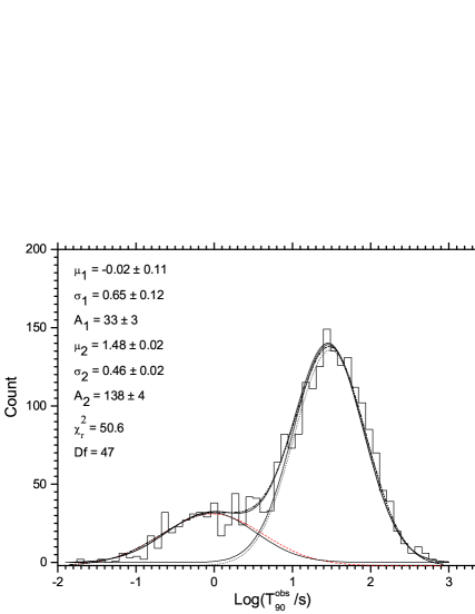
Fig. 1 : Observed Duration distribution of 2238 Fermi’s GRBs. The parameters A, $\mu$, and $\sigma$ characterize the Gaussian fit. N=2238 GRBs and the bin width is 0.09. The dotted lines correspond to the results of the $\chi^{2}_{r}$ method and the continuous lines correspond to the results obtained by log-likelihood method.

Although the $\chi^{2}_{r}$ minimization method depends strongly on the number of bins used (Huja et al., 2009; Tarnopolski, 2015a), it does give a good fit, similar to what is obtained using the log-likelihood function method. This is due to the large number of data points, which exceeds 2000, and the appropriate density of the data.

Table 1 : The distribution of the observed durations of 2238 Fermi GRBs represented by two and three Gaussian functions (two and three GRB groups). The parameters presented here are all defined in the main text.

	Two groups
i	1	2
f	$0.225\pm 0.005$	$0.775\pm 0.005$
$\mu$	$-0.04^{+0.22}_{-0.16}$	$1.46^{+0.07}_{-0.04}$
$\sigma$	$0.57^{+0.11}_{-0.03}$	$0.45^{+0.02}_{-0.03}$
$\ln{L}$	-2383.3
BIC	4805.2
AIC	4776.6
k	5

		Three groups
i	1	2	3
f	$0.13\pm 0.05$	$0.15\pm 0.13$	$0.72\pm 0.07$
$\mu$	$-0.29\pm 0.04$	$0.60^{+0.1}_{-0.4}$	$1.49\pm 0.07$
$\sigma$	$0.47^{+0.17}_{-0.05}$	$0.62\pm 0.13$	$0.44\pm 0.01$
$\ln{L}$	-2382.14
BIC	4825.99
AIC	4780.28
k	8

In a second step, we note that due to the uncertainties on $T_{90}^{Obs}$, bursts near the value of 2.0 s might be short or long, and thus the number of short Fermi/GBM bursts may vary between 289 and 451, and the number of long bursts may vary between 1787 and 1949. We thus limit ourselves to the 1787 bursts that are most probably long and the 289 ones that are most probably short. We eliminated 162 bursts in total, of which 151 were originally “short”, due to their large uncertainties, which made them potentially belong to either group. This procedure of strongly separating the two groups is done in order to estimate the intervals that cover the majority of the values of the spectra parameters ($\alpha$, $\beta$ and $E_{p}$) for each population, if we consider a two-group model. We use those intervals in our subsequent calculations in cases where the values of the spectral parameters given by the NASA website are tainted with a large uncertainty.

After applying the last filter, we plot in Figure (2) the distribution of durations of the remaining 2076 bursts. The fits are again obtained using both the minimization of the chi-square function and the maximization of the log-likelihood function (Table 2). A very slight difference is noted between the results from the two methods. We note that after removing the doubtful bursts, we obtain two populations that are clearly separate.

Fig. 2 : Observed Fermi/GBM durations of selected 2076 Fermi GRBs. The bin width is 0.09.

Table 2 : Central value, $\mu$, and variance $\sigma^{2}$ of the distribution of 2076’s Fermi duration. Here we use the same definitions as in Table (1).

	Two groups
i	1	2
f	0.139	0.861
$\mu$	-0.399	1.443
$\sigma$	0.377	0.453
$\ln{L}$	-2041.50
BIC	4121.20
AIC	4093.0
k	5

2.2 Fermi Distribution of $E_{p}$, $\alpha$ and $\beta$

Band et al. (1993) assumed that the spectrum of the gamma burst can be described by a function composed of two parts:

$N(E)=N_{0}\times$

$$\left\{\begin{split}&(\frac{E}{100\leavevmode\nobreak\ keV})^{\alpha}\exp(-\frac{E}{E_{0}})&,E\leq E_{b}\\ &(\frac{E_{b}}{100\leavevmode\nobreak\ keV})^{\alpha-\beta}\exp{[\beta-\alpha](\frac{E}{100\leavevmode\nobreak\ keV})^{\beta}}&,E>E_{b}\end{split}\right\}.$$ (7)

where $E_{b}=(\alpha-\beta)E_{0}$ and $E_{0}=\frac{E_{p}^{Obs}}{\alpha+2}$. $N(E)$ has units of photons $s^{-1}$ $keV^{-1}$ $cm^{-2}$.

We seek the values of $E_{p}^{obs}$, $\alpha$ and $\beta$ for the two samples of gamma-ray bursts that we selected above (those consisting of 289 short SGRBs and 1787 long LGRBs). Out of the 289 SGRBs, we find 238 with definite spectral parameters. Out of the 1787 LGRBs, 1605 have definite spectral parameters. We present the distributions of these quantities (as probability density functions, PDF) in Figures (3) and (4). In these graphical representations, we apply no filter.

We note that for the two types of bursts, the values of $\alpha$ generally fall in the range $(-2,2)$, while the values of $\beta$ are less than $-1$. The lowest values of $\beta$ can go beyond $-10$ ($20\%$ of the 238 SGRBs and $30\%$ of the 1605 LGRBs). The distributions of $E_{p}$ values as presented graphically in Figures (3) and (4) show that around $95\%$ of the bursts have $E_{p}$ energies in the range $[8,1000]$ keV.

In the calculations that we subsequently perform, we consider values for $\alpha$, $\beta$, and $E_{p}$ as shown in Table (3) for all groups/populations (short, intermediate, or long). These intervals have been adopted by taking into account the figures (3) and (4) as well as the limits from BATSE given in the catalog 5B (Goldstein et al., 2013) so that the resulting distributions are centered around the modes; for $E_{p}$ we take the Fermi detection range. The choice of our intervals, which are very close to those presented in the data of the fifth catalog of BATSE cover the majority of the bursts.

Table 3 : Ranges of the spectral parameters $\alpha$, $\beta$, and $E_{p}$, with their uncertainties.

parameter	Interval
$\alpha\pm\Delta\alpha$	[-2.0 , 1.0]
$\beta\pm\Delta\beta$	[-4.5 , -1.0]
$E_{p}\pm\Delta E_{p}(keV)$	[8 , 1000]

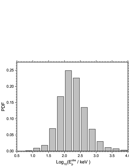
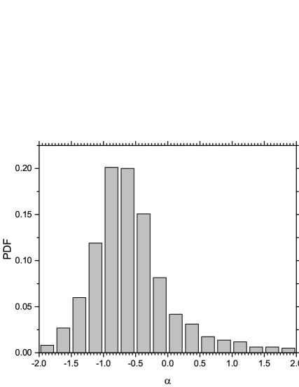
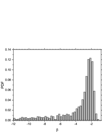
Fig. 3 : Distributions of $E_{p}^{obs}$, $\alpha$ and $\beta$ for a sample composed of 1605 Fermi LGRBs.

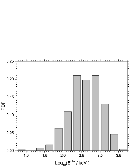
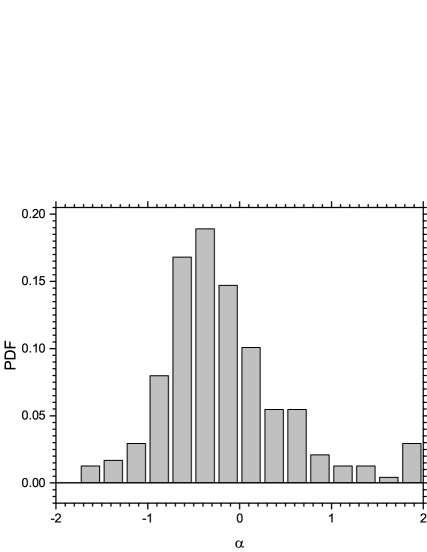
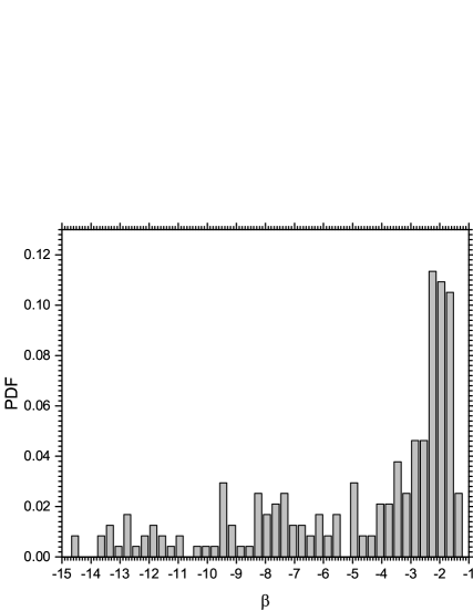
Fig. 4 : Distributions of $E_{p}^{obs}$, $\alpha$ and $\beta$ for a sample composed of 238 Fermi SGRBs.

3 Determination of Pseudo-Redshifts

As mentioned above, to address the dearth of redshifts and give ourselves a way to investigate intrinsic burst durations, we use correlation relations to determine pseudo-redshifts. This idea has been proposed and used several times in the past (e.g. (Atteia, 2003; Kocevski and Liang, 2003; Ghirlanda et al., 2005; Guidorzi, 2005; Guidorzi et al., 2006; Tsutsui et al., 2008, 2013; Zhang and Wang, 2018)). We delineate the method succinctly in the following sub-section.

3.1 Can correlation relations give correct redshifts?

We use a sample of Fermi bursts with known redshifts to assess the extent to which the correlation relations of Yonetoku et al. (2004, 2010) for long bursts and that of Tsutsui et al. (2013) for short bursts can produce correct redshifts.

The luminosity at the peak of the flux can be calculated using:

$${}\frac{L_{p}}{erg\leavevmode\nobreak\ s^{-1}}=4\pi D_{L}^{2}(z)\leavevmode\nobreak\ F_{\gamma}\leavevmode\nobreak\ k_{c},$$ (8)

where $L_{p}$ is k-corrected with the method developed by Bloom et al. (2001), and $k_{c}$ is the proper k-correction factor (Yonetoku et al., 2004; Rossi et al., 2008; Elliott et al., 2012; Zitouni et al., 2014) defined by:

$$k_{c}=\frac{\int_{E_{1}/(1+z)}^{E_{2}/(1+z)}EN(E)dE.}{\int_{E_{min}}^{E_{max}}EN(E)dE.},$$ (9)

where $[E_{1}=1\,keV;E_{2}=10^{4}\,keV]$ is the gamma radiation band in the source’s frame and $[E_{min}=8keV;E_{max}=10^{3}keV]$ is Fermi-detection interval.

The peak energy flux, denoted by $F_{\gamma}$ and calculated in $\mathrm{erg\,cm^{-2}\,s^{-1}}$, is calculated numerically through the following equation:

$$F_{\gamma}=\int_{E_{min}}^{E_{max}}EN(E)dE.$$ (10)

$D_{L}(z)$ is the luminosity distance, which is expressed by the following equation:

$$D_{L}=\frac{(1+z)c}{H_{0}}\int_{0}^{z}\frac{dz^{\prime}}{\sqrt{\Omega_{M}(1+z^{\prime})^{3}+\Omega_{\Lambda}}}.$$ (11)

$D_{L}(z)$ depends on the cosmological parameters $H_{0}$, $\Omega_{m}$, and $\Omega_{\Lambda}$. We consider a flat universe, where the values of these parameters are $70\leavevmode\nobreak\ km\,s^{-1}\,Mpc^{-1}$, 0.3, and 0.7.

For long bursts, the Yonetoku relation (Yonetoku et al., 2010) that we use is:

$${}\frac{L_{p}}{erg\leavevmode\nobreak\ s^{-1}}=10^{52.97}\leavevmode\nobreak\ [\frac{E_{p}^{obs}(1+z)}{774.5\leavevmode\nobreak\ keV}]^{1.60},$$ (12)

where $E_{p}^{obs}$ is the photon energy at the peak of the spectrum, measured in keV, and $E_{p}=E_{p}^{obs}(1+z)$ is the peak energy in the source’s frame.

For short bursts, the correlation relation (Tsutsui et al., 2013) that we use is (in the source frame):

$${}\frac{L_{p}}{erg\leavevmode\nobreak\ s^{-1}}=10^{52.29\pm 0.07}\leavevmode\nobreak\ [\frac{E_{p}^{obs}(1+z)}{774.5\leavevmode\nobreak\ keV}]^{1.59\pm 0.11}.$$ (13)

In order to validate these correlation relations and their capacity to determine redshifts, we use a sample of 117 Fermi bursts with known redshifts, which we give in Table (LABEL:tab3). A systematic and thorough search for redshifts of Fermi GRBs, including GCN telegrams, gave us 134 cases. This will surely increase in the future. The 134 GRBs were reduced to 117 bursts because the energy $E_{p}^{Obs}$ was sometimes outside of the Fermi detectors’ range $[8,1000]$ keV. The bursts that we eliminated are listed in Table (5).

Table 5 : 17 GRBs eliminated due to their $E_{p}^{Obs}$ falling outside of the Fermi detectors’ range $[8,1000]$ keV.

Name	z	$E_{b}^{Obs}$
		keV
GRB160623209	0.367	1032.9
GRB140809133	0.041	1078.76
GRB130215063	0.579	1210.92
GRB170604603	1.329	1285.12
GRB120711115	1.4	1357
GRB090902462	1.82	2152
GRB150120123	0.46	$<$10
GRB101213451	0.414
GRB171010792	0.3285
GRB090519881	3.85
GRB171222684	2.409
GRB100413732	4.0
GRB080905705	2.374
GRB120712571	4.1745
GRB170903534	0.886
GRB090510016	0.903
GRB171020813	1.87

We start by calculating the ratio of the luminosity $L_{p}$, which is obtained by using the relation (8), and the luminosity obtained using the correlation relations (12) or (13). This ratio, which we denote by $R_{L}$, is plotted in Figure (5) as a function of the redshift z. This was obtained using the data for $E_{p}^{Obs}$, $\alpha$, and $\beta$ found on the Fermi website.

When the ranges of the spectral parameters given in Table (3) are taken into account, our sample further reduces to 61 GRBs.

The quantity $R_{L}$ represents the quality of the correlation relation as a function of the redshift, the ideal situation being for $R_{L}=1.$ $R_{L}$ shows substantial dispersion in the data, although the data does show a correlation between the luminosity $L_{p}$ and the energy $E_{p}$ measured in the source frame. In Figure (5), we present $\log{R_{L}}$ vs. the redshift for the 61 GRBs (top panel), and a histogram of $\log{R_{L}}$ (bottom panel). We note that 55 points out of 61 (i.e. almost 90%) have an $R_{L}$ between 0.1 and 10. More than 67% of bursts have an $R_{L}$ between 0.3 and 3. The values of $\log{R_{L}}$ are given in Table (LABEL:tab3).

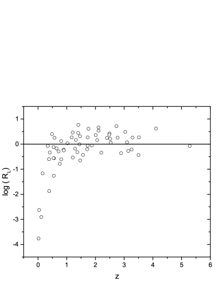
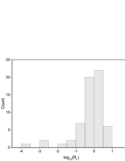
Fig. 5 : Top: $\log{R_{L}}$ (defined in the text) as a function of the redshift z for 61 GRBs. Bottom: Histogram of $\log{R_{L}}$. The values of $\log{R_{L}}$ are given in Table (LABEL:tab3).

It is also useful to study the evolution of the brightness in terms of the redshift for the 61 GRBs. We present this evolution graphically in Figure (6). This can also be analytically expressed by the following relation:

$$\frac{L_{p}}{10^{52.2\pm 0.1}\leavevmode\nobreak\ erg\,s^{-1}}=z^{2.0\pm 0.2}.$$ (14)

The evolution of the luminosity $L_{p}$ in terms of the redshift $z$ is important to note. For this relation, there is no difference between long and short bursts. The two bursts that are far from the “cloud” are GRB130427324 and GRB160625945; they have the two highest photon fluxes (523 $ph.\,cm^{-2}\,s^{-1}$ and 206 $ph.\,cm^{-2}\,s^{-1}$). It is then possible to use this relation to infer pseudo-redshifts. In other references, e.g. Lloyd-Ronning et al. (2002); Goldstein (2012); Salvaterra et al. (2012); Geng and Huang (2013); Zhang et al. (2014), a correlation is sought between $L_{p}$ and (1 + z) instead of z. We do not find the same slope at low redshift, but our results are in agreement at high redshifts. We do not focus on this issue, as it is not important in our present subject.

Fig. 6 : $L_{p}$ versus z for 61 Fermi GRBs with known redshifts. The values of $\log{R_{L}}$ are given in Table (LABEL:tab3).

As previously noted, our procedure for determining the pseudo-redshift, noted $z_{cal}$, is based on solving the equation (8)=(12) for long bursts and (8)=(13) for short bursts. We have followed the same approach as Zhang and Wang (2018).

To assess our method for the determination of pseudo-redshifts, we compare the values we determine ($z_{cal}$) with the measured redshift values ($z_{obs}$) for the sample of 61 GRBs. For that, we calculate the relative error, $\frac{\Delta z}{z}=\frac{\mid z_{cal}-z_{obs}\mid}{z_{obs}}$, for each burst, then we represent by a histogram (Fig.7) the number of cases having a relative uncertainty lower than a certain limit, which we vary from 0 to 1. We note that for a relative uncertainty less than 0.5, we get 31 redshifts out of 61, i.e. $\sim$ 51 %. Two-thirds of the pseudo-redshifts have a relative uncertainty of less than 0.70. This rather large error fraction is due to the large dispersion of the data ($\alpha$, $\beta$, $E_{p}$, and $P_{obs}$, the photon flux). In Fig. (8) we have plotted $z_{cal}$ vs. $z_{obs}$ for the 43 GRBs that have a relative uncertainty $\Delta z/z$ less than 80%.

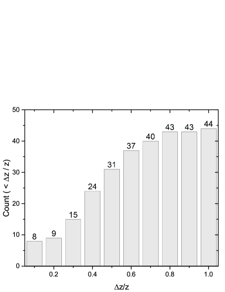
Fig. 7 : $\frac{\Delta z}{z}=\frac{|z_{cal}-z_{obs}|}{z_{obs}}$. ‘Count’ represents the cumulative number of GRBs that have a $\frac{\Delta z}{z}$ below the limit shown on the abscissa axis. Here we have used the sample of 61 GRBs.

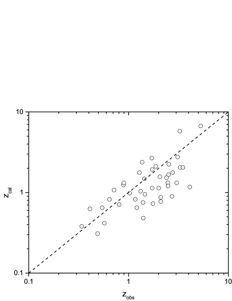
Fig. 8 : $z_{cal}$ vs. $z_{obs}$ for the 43 GRBs with $\frac{\Delta z}{z}<0.8$.

3.2 Redshift determination of Fermi GRBs

With the above validity tests of the method used to infer pseudo-redshifts, we adopt our calculated values as statistically valid substitutes for the actual redshifts $z$ for Fermi GRBs. We then take all the bursts recorded by the Fermi satellite since (the first one on) 14 July 2008 (GRB080714086) and up until 11 February 2018 (GRB180211754) (von Kienlin et al., 2014; Narayana Bhat et al., 2016) without any imposed condition.

This new sample comprises 2266 GRBs: 378 short ones and 1888 long ones. 243 GRBs lack one or more measured spectral parameter(s). Taking into account the ranges given in Table (3) for the spectral parameters eliminates more than 1000 GRBs.

When trying to obtain pseudo-redshifts, in a few cases the relevant equation has no solution, as the burst’s parameters ($\alpha,\beta,E_{p}$) and the flux place it far from the correlation line. In the end, we could determine pseudo-redshifts for 1017 GRBs (144 SGRBs and 873 LGRBs). However, we stress that while the values of the obtained pseudo-redshifts have large uncertainties and dispersions, their distribution conforms to that of the measured values (see also Fiore et al., 2007; Coward et al., 2013; Kanaan and de Freitas Pacheco, 2013; Wang and Dai, 2014). We plot the distribution of pseudo-redshifts in Figure (9) to show that it indeed concords with the distributions presented in previous works (Guetta and Piran, 2005; Bagoly et al., 2008; Jakobsson et al., 2012; Herbel et al., 2017). This important remark allows us to use the values of the pseudo-redshifts thus obtained in statistical studies, especially when the number of bursts is large, such as in our case. We should also stress, however, that the pseudo-redshifts thus obtained cannot be used for individual bursts, due to the large uncertainties that taint their determination.

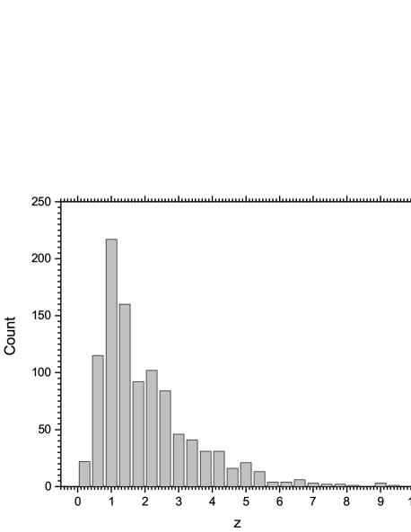
Fig. 9 : Pseudo-redshift distribution for 1017 Fermi GRBs. The bin width is 0.4.

We have also performed a validation of the results we have obtained for peudo-redshifts by the study of the Amati relation ($\frac{E_{p,r}}{keV}=K(\frac{E_{iso}}{10^{52}\leavevmode\nobreak\ erg})^{m}$). This is shown graphically in Figure (10).

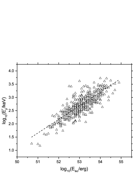
Fig. 10 : Amati relation for 873 Fermi long GRBs. The dashed line represents a linear fit given by the equation: $\log{(E_{p}^{r}/keV)}=(-24.6\pm 0.6)+(0.515\pm 0.012)\log{(E_{iso}/erg)}$

We obtain values for K and m that are close to those that we obtained in our previous work, which we conducted on Swift/BAT bursts (Zitouni et al., 2014). In Table (6); we also compare our results with the original ones of Amati et al. (2002), which were obtained using a sample consisting of only 9 bursts. Many works have produced parameters for the Amati relation, e.g. (Amati et al., 2008, 2009; Capozziello and Izzo, 2010). Our results are in very good agreement with all these works, particularly with regard to the slope $m$, which is generally given with good precision.

Table 6 : $E_{iso}-E_{p,r}$ correlation. Ref.1: Zitouni et al. (2014), Ref.2: Amati et al. (2002)

	This work	Ref.1	Ref.2
K	$151^{+2}_{-5}$	$141^{+18}_{-15}$	$\sim 95$
m	$0.515\pm 0.012$	$0.45\pm 0.10$	$0.52\pm 0.06$

4 Intrinsic Duration Distribution

In this section we determine the intrinsic (source frame) durations $T^{r}_{90}$ of Fermi GRBs, using the pseudo-redshifts obtained from the correlation relations. We study the distribution of $\log{(T^{r}_{90})}$, as had been done for the BATSE, Swift, and Fermi bursts (Zitouni et al., 2015; Shahmoradi and Nemiroff, 2015; Tarnopolski, 2016c; Zhang et al., 2016; Kulkarni and Desai, 2017).

The distribution of the intrinsic duration is studied in the same approach that we applied to the distribution of the observed durations. Indeed, we use the two statistical evaluation methods, namely the method of minimization of the $\chi^{2}_{r}$ function and the method of the maximization of the log-likelihood function.

The results of the log-likelihood method are presented in Table (7). The (previously defined) AIC and BIC both favor the two-group model over that of three groups. The parameters of each model are given in the two corresponding sub-tables. Figure (11) shows the results of the two statistical evaluations methods: those of the $\chi^{2}_{r}$ minimization method are shown by dotted lines, and those of the log-likelihood method are shown by continuous lines.

The two groups/populations have the following parameters: the durations of the peak bursts are (in the source frames): $0.24^{+0.19}_{-0.05}\leavevmode\nobreak\ s$ and $8.7^{+1.1}_{-1.8}\leavevmode\nobreak\ s$, respectively, and the logarithmic standard deviations are: $\sigma_{1}=0.44$ and $\sigma_{2}=0.50$ , respectively (Table 8). These values are calculated from the results of the likelihood method presented in the table ( ref tab6N).

Along with results from previous works (Zhang and Choi (2008) and, most recently, Zitouni et al. (2015)), and while we note some differences in the centroid values of the two populations between various works, we can state that this (and other) analysis(es) confirm(s) the existence of two populations of bursts as intrinsic and thus probably of inherently physical origin. The numbers of short and long bursts recorded by each instrument may be due to the time response of the detectors. Depending on the trigger criteria, some gamma-ray detectors may be more responsive to one class (LGRBs) over another (SGRBs) (Hakkila et al., 2003; Shahmoradi and Nemiroff, 2015).

Fig. 11 : Intrinsic duration distribution of 1017 Fermi GRBs. The parameters A, $\mu$, and $\sigma$ characterize the Gaussian fit. The bin width is 0.09.

Table 7 : The distribution of intrinsic durations of 1017 Fermi GRBs represented by two and three Gaussian functions (two and three groups of GRBs). The parameters presented here are all defined in the main text.

	Two groups
i	1	2
f	$0.136\pm 0.02$	$0.864\pm 0.02$
$\mu$	$-0.62^{+0.25}_{-0.10}$	$0.94^{+0.05}_{-0.04}$
$\sigma$	$0.442\pm 0.079$	$0.464\pm 0.022$
$\ln{L}$	-1055.239
BIC	2145.101
AIC	2120.478
k	5

		Three groups
i	1	2	3
f	$0.03^{+0.02}_{-0.01}$	$0.10^{+0.04}_{-0.02}$	$0.87^{+0.03}_{-0.06}$
$\mu$	$-1.03^{+0.06}_{-0.07}$	$-0.44^{+0.07}_{-0.06}$	$0.98^{+0.02}_{-0.05}$
$\sigma$	$0.36\pm 0.07$	$0.37\pm 0.09$	$0.497\pm 0.020$
$\ln{L}$	-1055.742
BIC	2166.882
AIC	2127.485
k	8

Table 8 : Position values of the centroids in the intrinsic duration distributions. Ref.1: Zitouni et al. (2015), Ref.2: Zhang and Choi (2008). $G_{1}$ and $G_{2}$ are the statistical parameters corresponding to the two groups/populations (SGRBs and LGRBs).

	This work	Ref.1	Ref.2
$G_{1}$	$0.24^{+0.19}_{-0.05}$	$0.13^{+0.05}_{-0.03}$	0.13
$G_{2}$	$8.7^{+1.1}_{-1.8}$	$16.4^{+1.2}_{-1.1}$	12.30

5 Results and conclusion

In this work, we have studied the distribution of the durations of Fermi gamma-ray bursts in their source frames as well as in the observer’s frame. To obtain the intrinsic (source frame) durations, we have assumed the validity of the correlation relations between the luminosity $L_{p}$ at the spectral peak and the energy $E_{p}$ at the flux peak. This assumption is needed in order to determine the pseudo-redshift of each burst, which then allows us to infer the burst’s duration in its source frame. However, while such pseudo-redshifts are often tainted by substantial uncertainties, their distribution remains close to that of the measured redshifts. This remark, coupled with the large number of bursts used in our study, encourages us to confidently use the pseudo-redshifts in studying the distributions of the bursts’ durations in their source frames. It is worth mentioning that the distributions of spectral parameters ($\alpha$, $\beta$ and $E_{p}^{Obs}$), which are used to infer peudo-redshifts from the correlation relations between $L_{p}$ and $E_{p}$, must give the same distribution as the measured redshifts. This is indeed the case when we assume the validity of the correlation relations.

In order to compare the distributions of the observed (measured) and intrinsic durations, we have determined pseudo-redshifts for 1017 bursts: 144 SGRBs and 873 LGRBs. The distribution of the observed durations of these bursts is shown in Figure (12) (the dashed lines). The fits (with Gaussian functions) were obtained by using the maximization of the log-likelihood function $\ln{L}$; here we adopt the two-group model for this comparison. The parameters describing the two groups/populations are given in Figure (12). The borderline between the two groups is in the interval [1.7, 2.5] s. Our results are in good agreement with the conclusions drawn by Bromberg et al. (2013) and Tarnopolski (2015b) for Fermi bursts. They confirm the separation between the two groups/populations around 2 seconds.

The distribution of intrinsic durations of the same sample is shown in the same figure (12) (the continuous lines). Likewise, the fit is obtained by maximization of the log-likelihood function. We find that two groups/populations of bursts characterize the distribution of durations quite well and are intrinsically separate.

We also note that the observed and intrinsic distributions are very similar, with a shift to the right ($2.0$ s compared to $1.0$ s) for the observed durations, due to the time dilation produced by the redshift/expansion of the universe. This is consistent with what was found by Tarnopolski (2016b) and Tarnopolski (2016c). The shift found here may be slightly different than what was found in those works, but that may be ascribed to different detector characteristics (Fermi vs. Swift/BAT).

Our analysis indicates that Fermi bursts can be represented by two groups/populations. The possibility of a third one had been raised in previous works (see Zitouni et al. (2014) and references therein) at least in some databases (Swift/BAT but not BATSE). We find that a third component is not needed to describe the Fermi GRB durations. Thus the issue of detector characteristics seems to be the main factor in this regard, as we had suggested (Zitouni et al. (2014)).

Finally, the 2.0-second dividing line (for observed durations) also seems to be somewhat arbitrary and detector/instrument-dependent; for intrinsic durations, a separation around 1.0 second seems to apply, with this value being largely approximate.

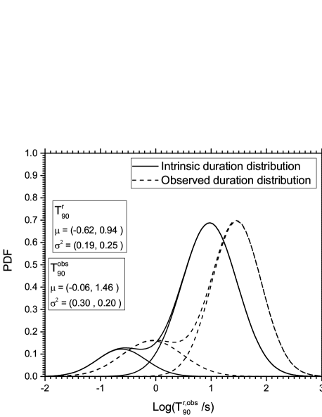
Fig. 12 : Density of the function of distribution of observed and intrinsic durations. The sample used here is composed of 1017 Fermi GRBS.

Acknowledgements The research reported in this publication was supported by the Mohammed Bin Rashid Space Centre (MBRSC), Dubai, UAE, under Grant ID number 201603.SS.AUS. The authors also acknowledge the use of the online Fermi/GBM table compiled by von Kienlin et al. (2014) and Narayana Bhat et al. (2016). HZ wishes to thank the American University of Sharjah (UAE) for hosting him for two weeks, during which part of this work was conducted. The authors thank the anonymous referee for very useful comments, which led to significant improvements of the paper.

Table 4 : Data for the 117 Fermi GRBs that were used to validate the determination of pseudo-redshifts. 61 GRBs are used in our calculations, the remaining 56 GRBs are eliminated because of their spectral parameters which are found outside the chosen intervals. $F_{\gamma}$ and $L_{p}$ are calculated in this work.

GRB	$z_{obs}$	$T_{90}^{obs}$	$E_{p}^{obs}$	$\alpha$	$\beta$	$\log{(F_{\gamma})}$	$\log{(L_{p})}$	$\log(R_{L})$	$z_{cal}$
		(s)	(keV)			($erg\,cm^{-2}\,s^{-1}$)	($erg\,s^{-1}$)
GRB170705115	2.01	22.78	167 $\pm$ 15	-0.694 $\pm$ 0.09	-2.44 $\pm$ 0.25	-5.5	53.03	0.36	1.14
GRB170607971	0.557	22.59	131 $\pm$ 27	-1.18 $\pm$ 0.13	-2.13 $\pm$ 0.2	-5.8	51.48	-0.562	1.20
GRB170405777	3.51	78.59	324 $\pm$ 41	-0.674 $\pm$ 0.07	-2.25 $\pm$ 0.32	-5.5	53.68	0.268	2.05
GRB170214649	2.53	122.88	455 $\pm$ 74	-0.695 $\pm$ 0.07	-1.96 $\pm$ 0.12	-5.4	53.53	0.057	2.24
GRB160821937	0.16	1.09	125 $\pm$ 76	-0.663 $\pm$ 0.65	-2.41 $\pm$ 1.11	-6	49.97	-1.167	0.67
GRB160625945	1.406	454.67	594 $\pm$ 15	-0.502 $\pm$ 0.01	-2.05 $\pm$ 0.02	-4.2	54.16	0.767	0.48
GRB160509374	1.17	369.67	345 $\pm$ 14	-0.752 $\pm$ 0.02	-2.25 $\pm$ 0.06	-4.8	53.21	0.267	0.82
GRB151111356	3.5	46.34	108 $\pm$ 44	0.311 $\pm$ 1.15	-2.77 $\pm$ 1.78	-6.9	52.21	-0.437	11.06
GRB151027166	0.81	123.39	224 $\pm$ 46	-0.855 $\pm$ 0.11	-2.05 $\pm$ 0.17	-5.8	51.91	-0.608	2.18
GRB150821406	0.755	103.43	291 $\pm$ 52	-0.843 $\pm$ 0.09	-2.13 $\pm$ 0.21	-5.7	51.89	-0.787	2.76
GRB150514774	0.807	10.81	55 $\pm$ 4	-0.765 $\pm$ 0.15	-2.77 $\pm$ 0.19	-5.9	51.66	0.12	0.71
GRB150403913	2.06	22.27	509 $\pm$ 34	-0.672 $\pm$ 0.03	-2.19 $\pm$ 0.08	-5	53.61	0.155	1.57
GRB150314205	1.758	10.69	298 $\pm$ 9	-0.406 $\pm$ 0.03	-2.54 $\pm$ 0.08	-4.8	53.62	0.61	0.73
GRB141121414	1.47	3.84	144 $\pm$ 36	0.538 $\pm$ 0.71	-2.4 $\pm$ 0.66	-6.4	51.78	-0.65	5.44
GRB141004973	0.573	2.56	31 $\pm$ 10	0.43 $\pm$ 1.47	-1.88 $\pm$ 0.07	-6	51.31	0.25	0.42
GRB140907672	1.21	35.84	101 $\pm$ 20	-0.511 $\pm$ 0.32	-2.7 $\pm$ 0.73	-6.4	51.57	-0.534	3.01
GRB140817293	0.018	16.13	132 $\pm$ 21	-0.464 $\pm$ 0.24	-2.67 $\pm$ 0.45	-5.9	47.99	-3.763	1.82
GRB140808038	3.29	4.48	144 $\pm$ 14	-0.107 $\pm$ 0.17	-3.01 $\pm$ 0.62	-5.9	53.07	0.262	2.05
GRB140801792	1.32	7.17	122 $\pm$ 4	0.045 $\pm$ 0.08	-4.05 $\pm$ 0.8	-5.6	52.44	0.167	1.04
GRB140703026	3.14	83.97	232 $\pm$ 69	-0.699 $\pm$ 0.21	-2.34 $\pm$ 0.66	-6.2	52.85	-0.273	6.31
GRB140508128	1.027	44.29	369 $\pm$ 20	-0.55 $\pm$ 0.04	-2.37 $\pm$ 0.09	-4.9	52.98	0.034	0.98
GRB140506880	0.889	64.13	138 $\pm$ 21	-0.484 $\pm$ 0.21	-2.43 $\pm$ 0.25	-5.7	51.99	-0.218	1.24
GRB140423356	3.26	95.23	176 $\pm$ 86	-0.486 $\pm$ 0.46	-2.06 $\pm$ 0.51	-6.3	52.74	-0.214	5.77
GRB140304557	5.283	31.23	165 $\pm$ 92	-0.56 $\pm$ 0.53	-2.06 $\pm$ 0.57	-6.4	53.1	-0.075	6.69
GRB140213807	1.208	18.62	84 $\pm$ 3	-0.844 $\pm$ 0.06	-2.89 $\pm$ 0.17	-5.5	52.44	0.461	0.65
GRB140206304	2.73	27.26	112 $\pm$ 7	0.641 $\pm$ 0.21	-2.5 $\pm$ 0.12	-5.6	53.26	0.718	0.90
GRB131231198	0.644	31.23	313 $\pm$ 11	-0.792 $\pm$ 0.02	-2.66 $\pm$ 0.11	-4.8	52.52	-0.17	0.82
GRB131108862	2.4	18.18	333 $\pm$ 35	-0.598 $\pm$ 0.07	-1.94 $\pm$ 0.07	-5.3	53.48	0.245	1.53
GRB131011741	1.874	77.06	168 $\pm$ 88	-0.472 $\pm$ 0.43	-1.63 $\pm$ 0.12	-6.1	52.59	-0.054	2.11
GRB130518580	2.488	48.58	467 $\pm$ 31	-0.75 $\pm$ 0.03	-2.15 $\pm$ 0.07	-4.9	53.91	0.424	1.20
GRB130427324	0.34	138.24	718 $\pm$ 6	-0.454 $\pm$ 0.01	-3.13 $\pm$ 0.04	-3.7	53.05	-0.072	0.38
GRB121031949	0.113	242.44	300 $\pm$ 98	-0.693 $\pm$ 0.21	-2.74 $\pm$ 1.97	-6.1	49.48	-2.905	10.12
GRB120922939	3.1	182.28	65 $\pm$ 24	-1.047 $\pm$ 0.62	-2.48 $\pm$ 0.61	-6.7	52.3	0.07	2.76
GRB120716712	2.48	237.06	106 $\pm$ 17	-0.389 $\pm$ 0.22	-2.14 $\pm$ 0.17	-6	52.83	0.374	1.31
GRB120119170	1.728	55.3	274 $\pm$ 32	-0.842 $\pm$ 0.06	-2.35 $\pm$ 0.24	-5.5	52.88	-0.066	1.93
GRB111228657	0.716	99.84	95 $\pm$ 12	-1.374 $\pm$ 0.08	-2.73 $\pm$ 0.51	-5.9	51.6	-0.289	1.07
GRB111107035	2.893	12.03	129 $\pm$ 76	-0.649 $\pm$ 0.73	-2.55 $\pm$ 1.63	-6.6	52.31	-0.36	6.69
GRB110721200	0.382	21.82	225 $\pm$ 18	-0.64 $\pm$ 0.05	-1.93 $\pm$ 0.04	-5.2	51.73	-0.6	0.84
GRB110213220	1.46	34.3	81 $\pm$ 10	-1.059 $\pm$ 0.13	-2.67 $\pm$ 0.37	-5.9	52.34	0.311	0.95
GRB101219686	0.552	51.01	87 $\pm$ 23	0.496 $\pm$ 0.98	-2.64 $\pm$ 0.85	-6.6	50.5	-1.261	4.05
GRB100906576	1.727	110.59	146 $\pm$ 25	-0.603 $\pm$ 0.16	-2.14 $\pm$ 0.16	-5.7	52.78	0.268	1.15
GRB100814160	1.44	150.53	128 $\pm$ 29	0.911 $\pm$ 0.72	-1.84 $\pm$ 0.14	-6	52.33	-0.007	1.48
GRB100728439	2.106	10.24	63 $\pm$ 21	-0.178 $\pm$ 0.62	-1.84 $\pm$ 0.12	-6.1	52.55	0.535	0.87
GRB100728095	1.567	165.38	446 $\pm$ 56	-0.454 $\pm$ 0.09	-2.47 $\pm$ 0.38	-5.5	52.81	-0.429	3.60
GRB100724029	1.288	114.69	472 $\pm$ 39	-0.67 $\pm$ 0.04	-2 $\pm$ 0.07	-5.2	53.02	-0.179	1.77
GRB100615083	1.398	37.38	48 $\pm$ 7	0.311 $\pm$ 0.5	-2.12 $\pm$ 0.1	-6.1	52.09	0.445	0.75
GRB100414097	1.368	26.5	478 $\pm$ 40	-0.724 $\pm$ 0.04	-2.52 $\pm$ 0.26	-5.3	52.92	-0.318	2.38
GRB100216422	0.038	0.19	510 $\pm$ 382	0.036 $\pm$ 0.82	-1.72 $\pm$ 0.28	-5.6	49.4	-2.624	1.01
GRB100206563	0.41	0.18	566 $\pm$ 117	-0.222 $\pm$ 0.18	-2.38 $\pm$ 0.45	-5	51.97	-0.336	0.63
GRB091127976	0.49	8.7	55 $\pm$ 2	-0.509 $\pm$ 0.08	-2.27 $\pm$ 0.03	-5.3	51.81	0.4	0.31
GRB091020900	1.71	24.26	240 $\pm$ 143	-0.912 $\pm$ 0.26	-1.68 $\pm$ 0.09	-5.9	52.65	-0.202	2.68
GRB091003191	0.897	20.22	390 $\pm$ 25	-0.596 $\pm$ 0.04	-2.33 $\pm$ 0.11	-5.1	52.69	-0.252	1.32
GRB090926181	2.106	13.76	349 $\pm$ 9	-0.464 $\pm$ 0.02	-2.7 $\pm$ 0.1	-4.7	53.87	0.664	0.77
GRB090618353	0.54	112.39	426 $\pm$ 24	-0.958 $\pm$ 0.03	-2.87 $\pm$ 0.26	-4.9	52.29	-0.56	1.17
GRB090516353	4.109	123.07	70 $\pm$ 50	-0.555 $\pm$ 0.92	-1.79 $\pm$ 0.15	-6.3	53.05	0.621	1.16
GRB090424592	0.544	14.14	187 $\pm$ 6	-0.843 $\pm$ 0.02	-2.94 $\pm$ 0.16	-5	52.17	-0.119	0.65
GRB081222204	2.77	18.88	167 $\pm$ 19	-0.735 $\pm$ 0.09	-2.59 $\pm$ 0.38	-5.8	53.08	0.257	1.77
GRB081121858	2.512	41.98	192 $\pm$ 66	-0.195 $\pm$ 0.44	-1.76 $\pm$ 0.1	-5.8	53.08	0.209	1.67
GRB081025349	0.39	22.53	406 $\pm$ 122	-0.415 $\pm$ 0.22	-2.77 $\pm$ 2.21	-6	50.87	-1.875	0.02
GRB081028538	3.038	13.31	64 $\pm$ 9	0.171 $\pm$ 0.45	-2.48 $\pm$ 0.24	-6.2	52.7	0.49	1.32
GRB080804972	2.205	24.7	163 $\pm$ 32	-0.189 $\pm$ 0.28	-2.8 $\pm$ 1.14	-6.3	52.35	-0.342	4.42
GRB170817529	0.01	2.05	177 $\pm$ 99	1.728 $\pm$ 2.99	-2.47 $\pm$ 1.47
GRB170714049	0.793	0.22	487 $\pm$ 127	0.539 $\pm$ 0.68	-17.62 $\pm$ 5840000
GRB170428136	0.454	30.46	131 $\pm$ 42	-0.568 $\pm$ 0.39	-7.53 $\pm$ 1366.51
GRB170113420	1.968	49.15	235 $\pm$ 574	-1.354 $\pm$ 0.71	-1.96 $\pm$ 0.72
GRB161129300	0.645	36.1	276 $\pm$ 59	-0.878 $\pm$ 0.14	-13.78 $\pm$ 1630000
GRB161117066	1.549	122.18	71 $\pm$ 7	-0.813 $\pm$ 0.18	4.06 $\pm$ 29.21
GRB161017745	2.013	32.26	417 $\pm$ 138	-1.23 $\pm$ 0.14	-5.1 $\pm$ 123.83
GRB161014522	2.823	36.61	202 $\pm$ 27	-0.518 $\pm$ 0.13	-11.96 $\pm$ 154897.1
GRB161001045	0.891	2.24	442 $\pm$ 57	-0.726 $\pm$ 0.09	-13.31 $\pm$ 349696
GRB160804065	0.736	131.59	87 $\pm$ 59	-1.019 $\pm$ 0.42	-2.03 $\pm$ 3.25
GRB160624477	0.483	0.45	678 $\pm$ 258	0.115 $\pm$ 0.59	-19.11 $\pm$ 39570000
GRB160314473	0.727	1.66	709 $\pm$ 989	-1.181 $\pm$ 0.33	-5.12 $\pm$ 226.2
GRB160228034	1.64	16.13	16 $\pm$ 119	-0.589 $\pm$ 35.32	-1.9 $\pm$ 0.2
GRB160227831	2.38	7.68	511 $\pm$ 36	-0.347 $\pm$ 0.07	-18.63 $\pm$ 21200000
GRB150727793	0.313	49.41	86 $\pm$ 54	1.732 $\pm$ 3.6	-1.7 $\pm$ 0.19
GRB150512432	0.104	123.14	219 $\pm$ 36	-0.776 $\pm$ 0.15	-11.29 $\pm$ 84293.06
GRB150424403	0.3	36.1	148 $\pm$ 53	-1.049 $\pm$ 0.25	-3.49 $\pm$ 8.65
GRB150301818	1.517	13.31	174 $\pm$ 37	-0.952 $\pm$ 0.17	-8.47 $\pm$ 5166.64
GRB150101641	0.134	0.08	23 $\pm$ 5	1.161 $\pm$ 2.95	-1.6 $\pm$ 1.08
GRB141225959	0.915	56.32	145 $\pm$ 47	1.021 $\pm$ 1.12	-1.95 $\pm$ 0.27
GRB141221338	1.452	23.81	321 $\pm$ 114	-1.075 $\pm$ 0.15	-6.32 $\pm$ 663.11
GRB141220252	1.32	7.62	215 $\pm$ 13	-0.525 $\pm$ 0.07	-6.88 $\pm$ 114.6
GRB141118678	0.108	4.35	317 $\pm$ 41	-0.536 $\pm$ 0.12	-13.97 $\pm$ 789873.6
GRB140606133	0.384	22.78	881 $\pm$ 350	-1.268 $\pm$ 0.06	0.28 $\pm$ 5.54
GRB140512814	0.725	147.97	575 $\pm$ 95	-1 $\pm$ 0.06	-4.37 $\pm$ 15.75
GRB140311885	4.954	72.19	353 $\pm$ 290	-1.138 $\pm$ 0.3	-6.96 $\pm$ 4223.74
GRB140219824	0.12	77.06	32 $\pm$ 19	1.534 $\pm$ 3.98	-1.76 $\pm$ 0.15
GRB131105087	1.686	112.64	453 $\pm$ 76	-1.032 $\pm$ 0.06	-16.38 $\pm$ 14810000
GRB131004904	0.717	1.15	144 $\pm$ 90	-1.254 $\pm$ 0.46	-19.41 $\pm$ 3.146e+09
GRB130925173	0.347	215.56	94 $\pm$ 12	-1.305 $\pm$ 0.12	-6.4 $\pm$ 270.65
GRB130702004	0.145	58.88	13 $\pm$ 54	2.078 $\pm$ 85.25	-1.75 $\pm$ 0.05
GRB130612141	2.006	7.42	23 $\pm$ 7	4.747 $\pm$ 7.92	-2.15 $\pm$ 0.18
GRB130610133	2.092	21.76	150 $\pm$ 56	-1.089 $\pm$ 0.3	-18 $\pm$ 679300000
GRB130420313	1.297	104.96	59 $\pm$ 6	-0.03 $\pm$ 0.58	-21.3 $\pm$ 425600000
GRB121211574	1.023	5.63	111 $\pm$ 45	-0.645 $\pm$ 0.54	-3 $\pm$ 3.08
GRB121128212	2.2	17.34	115 $\pm$ 7	-0.459 $\pm$ 0.11	-15.64 $\pm$ 2160000
GRB121123421	2.7	102.34	164 $\pm$ 26	-0.384 $\pm$ 0.26	-8.77 $\pm$ 2722.15
GRB120909070	3.93	112.07	705 $\pm$ 361	-0.912 $\pm$ 0.16	-2.75 $\pm$ 3.13
GRB120907017	0.97	5.76	134 $\pm$ 43	-0.936 $\pm$ 0.3	-8.88 $\pm$ 12518.22
GRB120811649	2.671	14.34	33 $\pm$ 6	4.591 $\pm$ 4.37	-2.23 $\pm$ 0.16
GRB120729456	0.8	25.47	27 $\pm$ 234	-0.053 $\pm$ 38.57	-1.63 $\pm$ 0.08
GRB120118709	2.943	37.83	67 $\pm$ 13	-0.932 $\pm$ 0.35	-5.94 $\pm$ 145.97
GRB110818860	3.36	67.07	55 $\pm$ 34	1.246 $\pm$ 2.92	-1.64 $\pm$ 0.12
GRB110128073	2.339	12.16	323 $\pm$ 207	-0.899 $\pm$ 0.34	-13.28 $\pm$ 2544000
GRB110106893	0.618	35.52	354 $\pm$ 306	-1.187 $\pm$ 0.28	-7.38 $\pm$ 7202.92
GRB100816026	0.805	2.04	132 $\pm$ 24	-0.13 $\pm$ 0.33	2.17 $\pm$ 1.39
GRB091024372	1.092	93.95	652 $\pm$ 972	-1.209 $\pm$ 0.42	-2.66 $\pm$ 4.39
GRB090927422	1.37	0.51	96 $\pm$ 15	2 $\pm$ 1.56	-10.93 $\pm$ 2663.18
GRB090926914	1.24	55.55	111 $\pm$ 14	-0.121 $\pm$ 0.32	-6.25 $\pm$ 76.75
GRB090423330	8	7.17	80 $\pm$ 21	-0.616 $\pm$ 0.54	-7.86 $\pm$ 1923.03
GRB090328401	0.736	61.7	458 $\pm$ 35	-0.784 $\pm$ 0.04	-4.45 $\pm$ 7.14
GRB090102122	1.547	26.62	378 $\pm$ 23	-0.274 $\pm$ 0.07	-7.32 $\pm$ 157.82
GRB081008832	1.969	150.01	173 $\pm$ 49	-0.662 $\pm$ 0.3	-12.3 $\pm$ 434886.5
GRB080928628	1.69	14.34	83 $\pm$ 33	-1.139 $\pm$ 0.45	-2.92 $\pm$ 2.52
GRB080916406	0.689	46.34	241 $\pm$ 37	-0.428 $\pm$ 0.17	-4.83 $\pm$ 20.44
GRB080810549	3.35	107.46	735 $\pm$ 489	-1.18 $\pm$ 0.14	-2.43 $\pm$ 1.75

References

- Abbott et al. (2017a) Abbott, B.P., Abbott, R., Abbott, T.D., Acernese, F., Ackley, K., Adams, C., Adams, T., Addesso, P., Adhikari, R.X., Adya, V.B., et al.: Astrophys. J. Lett. 848, 13 (2017a). 1710.05834. doi:10.3847/2041-8213/aa920c
- Abbott et al. (2017b) Abbott, B.P., Abbott, R., Abbott, T.D., Acernese, F., Ackley, K., Adams, C., Adams, T., Addesso, P., Adhikari, R.X., Adya, V.B., et al.: Astrophys. J. Lett. 848, 12 (2017b). 1710.05833. doi:10.3847/2041-8213/aa91c9
- Akaike (1974) Akaike, H.: IEEE Transactions on Automatic Control 19, 716 (1974)
- Amati et al. (2009) Amati, L., Frontera, F., Guidorzi, C.: Astron. Astrophys. 508, 173 (2009). 0907.0384. doi:10.1051/0004-6361/200912788
- Amati et al. (2002) Amati, L., Frontera, F., Tavani, M., in’t Zand, J.J.M., Antonelli, A., Costa, E., Feroci, M., Guidorzi, C., Heise, J., Masetti, N., Montanari, E., Nicastro, L., Palazzi, E., Pian, E., Piro, L., Soffitta, P.: Astron. Astrophys. 390, 81 (2002). arXiv:astro-ph/0205230. doi:10.1051 /0004-6361:20020722
- Amati et al. (2008) Amati, L., Guidorzi, C., Frontera, F., Della Valle, M., Finelli, F., Landi, R., Montanari, E.: Mon. Not. R. Astron. Soc. 391, 577 (2008). 0805.0377. doi:10.1111/j.1365-2966.2008.13943.x
- Andrae et al. (2010) Andrae, R., Schulze-Hartung, T., Melchior, P.: ArXiv e-prints (2010). 1012.3754
- Atteia (2003) Atteia, J.-L.: Astron. Astrophys. 407, 1 (2003). astro-ph/0304327. doi:10.1051/0004-6361:20030958
- Bagoly et al. (2008) Bagoly, Z., Balázs, L., Horváth, I., Kelemen, J., Mészáros, A., Veres, P., Tusnády, G.: In: Huang, Y.-F., Dai, Z.-G., Zhang, B. (eds.) American Institute of Physics Conference Series. American Institute of Physics Conference Series, vol. 1065, p. 119 (2008). 0901.0103. doi:10.1063/1.3027895
- Balastegui et al. (2001) Balastegui, A., Ruiz-Lapuente, P., Canal, R.: Mon. Not. R. Astron. Soc. 328, 283 (2001). astro-ph/0108272. doi:10.1046/j.1365-8711.2001.04888.x
- Band et al. (1993) Band, D., Matteson, J., Ford, L., Schaefer, B., Palmer, D., Teegarden, B., Cline, T., Briggs, M., Paciesas, W., Pendleton, G., Fishman, G., Kouveliotou, C., Meegan, C., Wilson, R., Lestrade, P.: Astrophys. J. 413, 281 (1993). doi:10.1086/172995
- Bloom et al. (2001) Bloom, J.S., Frail, D.A., Sari, R.: Astron. J. 121, 2879 (2001). astro-ph/0102371. doi:10.1086/321093
- Bromberg et al. (2013) Bromberg, O., Nakar, E., Piran, T., Sari, R.: Astrophys. J. 764, 179 (2013). 1210.0068. doi:10.1088/0004-637X/764/2/179
- Burnham and Anderson (2004) Burnham, K.P., Anderson, D.R.: Sociological Methods & Research 33(2), 261 (2004). doi:10.1177 / 0049124104268644
- Capozziello and Izzo (2010) Capozziello, S., Izzo, L.: Astron. Astrophys. 519, 73 (2010). 1003.5319. doi:10.1051/0004-6361/201014522
- Chattopadhyay and Maitra (2017) Chattopadhyay, S., Maitra, R.: Mon. Not. R. Astron. Soc. 469, 3374 (2017). 1703.07338. doi:10.1093/mnras/stx1024
- Chattopadhyay et al. (2007) Chattopadhyay, T., Misra, R., Chattopadhyay, A.K., Naskar, M.: Astrophys. J. 667, 1017 (2007). 0705.4020. doi:10.1086/520317
- Coward et al. (2013) Coward, D.M., Howell, E.J., Branchesi, M., Stratta, G., Guetta, D., Gendre, B., Macpherson, D.: Mon. Not. R. Astron. Soc. 432, 2141 (2013). 1210.2488. doi:10.1093/mnras/stt537
- Elliott et al. (2012) Elliott, J., Greiner, J., Khochfar, S., Schady, P., Johnson, J.L., Rau, A.: Astron. Astrophys. 539, 113 (2012). 1202.1225. doi:10.1051/0004-6361/201118561
- Fiore et al. (2007) Fiore, F., Guetta, D., Piranomonte, S., D’Elia, V., Antonelli, L.A.: Astron. Astrophys. 470, 515 (2007). 0704.2189
- Geng and Huang (2013) Geng, J.J., Huang, Y.F.: Astrophys. J. 764, 75 (2013). 1212.4340. doi:10.1088/0004-637X/764/1/75
- Ghirlanda et al. (2005) Ghirlanda, G., Ghisellini, G., Firmani, C.: Mon. Not. R. Astron. Soc. 361, 10 (2005). astro-ph/0502186. doi:10.1111/ j.1745-3933.2005.00053.x
- Goldstein et al. (2013) Goldstein, A., Preece, R.D., Mallozzi, R.S., Briggs, M.S., Fishman, G.J., Kouveliotou, C., Pacieses, W.S., Burgess, J.M.: Astrophys. J. Suppl. 208, 21 (2013). 1311.7135. doi:10.1088/0067-0049/208/2/21
- Goldstein (2012) Goldstein, A.: The use of the bulk properties of gamma-ray burst prompt emission spectra for the study of cosmology. PhD thesis (2012). https://search.proquest.com/docview/1286783946?accountid=192290
- Guetta and Piran (2005) Guetta, D., Piran, T.: Astron. Astrophys. 435, 421 (2005). astro-ph/0407429. doi:10.1051/0004-6361:20041702
- Guidorzi (2005) Guidorzi, C.: Mon. Not. R. Astron. Soc. 364, 163 (2005). astro-ph/0508483. doi:10.1111/j.1365-2966.2005.09545.x
- Guidorzi et al. (2006) Guidorzi, C., Frontera, F., Montanari, E., Rossi, F., Amati, L., Gomboc, A., Mundell, C.G.: Mon. Not. R. Astron. Soc. 371, 843 (2006). astro-ph/0606526. doi:10.1111/j.1365-2966.2006.10717.x
- Hakkila et al. (2003) Hakkila, J., Giblin, T.W., Roiger, R.J., Haglin, D.J., Paciesas, W.S., Meegan, C.A.: Astrophys. J. 582, 320 (2003). astro-ph/0209073. doi:10.1086/344568
- Herbel et al. (2017) Herbel, J., Kacprzak, T., Amara, A., Refregier, A., Bruderer, C., Nicola, A.: J. Cosmol. Astropart. Phys. 8, 035 (2017). 1705.05386. doi:10.1088/1475-7516/2017/08/035
- Horváth (1998) Horváth, I.: Astrophys. J. 508, 757 (1998). astro-ph/ 9803077. doi:10.1086/306416
- Horváth et al. (2008) Horváth, I., Balázs, L.G., Bagoly, Z., Veres, P.: Astron. Astrophys. 489, 1 (2008). 0808.1067. doi:10.1051/0004-6361:200810269
- Huja et al. (2009) Huja, D., Mészáros, A., Řípa, J.: Astron. Astrophys. 504, 67 (2009). 0905.4821. doi:10.1051/0004-6361/200809802
- Jakobsson et al. (2012) Jakobsson, P., Hjorth, J., Malesani, D., Chapman, R., Fynbo, J.P.U., Tanvir, N.R., Milvang, B., Vreeswijk, P.M., Letawe, G., Starling, R.L.C.: Astrophys. J. 752, 62 (2012). 1205.3490. doi:10.1088/0004-637X/752/1/62
- Kanaan and de Freitas Pacheco (2013) Kanaan, C., de Freitas Pacheco, J.A.: Astron. Astrophys. 559, 64 (2013). 1309.1399. doi:10.1051/0004-6361 /201321963
- Kass and Raftery (1995) Kass, R.E., Raftery, A.E.: Journal of the American Statistical Association 90(430), 773 (1995). doi:10.1080/ 01621459.1995.10476572
- Klebesadel et al. (1973) Klebesadel, R.W., Strong, I.B., Olson, R.A.: Astrophys. J. Lett. 182, 85 (1973). doi:10.1086/181225
- Kocevski and Liang (2003) Kocevski, D., Liang, E.: Astrophys. J. 594, 385 (2003). astro-ph/0207052. doi:10.1086/376868
- Koshut et al. (1995) Koshut, T.M., Paciesas, W.S., Kouveliotou, C., van Paradijs, J., Pendleton, G.N., Fishman, G.J., Meegan, C.A.: In: American Astronomical Society Meeting Abstracts #186. Bulletin of the American Astronomical Society, vol. 27, p. 886 (1995)
- Kouveliotou et al. (1993) Kouveliotou, C., Meegan, C.A., Fishman, G.J., Bhat, N.P., Briggs, M.S., Koshut, T.M., Paciesas, W.S., Pendleton, G.N.: Astrophys. J. Lett. 413, 101 (1993). doi:10.1086/186969
- Kulkarni and Desai (2017) Kulkarni, S., Desai, S.: Astrophys. Space Sci. 362, 70 (2017). 1612.08235. doi:10.1007/s10509-017-3047-6
- Lloyd-Ronning et al. (2002) Lloyd-Ronning, N.M., Fryer, C.L., Ramirez-Ruiz, E.: Astrophys. J. 574, 554 (2002). astro-ph/0108200. doi:10.1086 /341059
- Metzger et al. (1997) Metzger, M.R., Djorgovski, S.G., Kulkarni, S.R., Steidel, C.C., Adelberger, K.L., Frail, D.A., Costa, E., Frontera, F.: Nature 387, 878 (1997). doi:10.1038/43132
- Narayana Bhat et al. (2016) Narayana Bhat, P., Meegan, C.A., von Kienlin, A., Paciesas, W.S., Briggs, M.S., Burgess, J.M., Burns, E., Chaplin, V., Cleveland, W.H., Collazzi, A.C., Connaughton, V., Diekmann, A.M., Fitzpatrick, G., Gibby, M.H., Giles, M.M., Goldstein, A.M., Greiner, J., Jenke, P.A., Kippen, R.M., Kouveliotou, C., Mailyan, B., McBreen, S., Pelassa, V., Preece, R.D., Roberts, O.J., Sparke, L.S., Stanbro, M., Veres, P., Wilson-Hodge, C.A., Xiong, S., Younes, G., Yu, H.-F., Zhang, B.: Astrophys. J. Suppl. Ser. 223, 28 (2016). 1603.07612. doi:10.3847/0067-0049/223/2/28
- Rossi et al. (2008) Rossi, F., Guidorzi, C., Amati, L., Frontera, F., Romano, P., Campana, S., Chincarini, G., Montanari, E., Moretti, A., Tagliaferri, G.: Mon. Not. R. Astron. Soc. 388, 1284 (2008). 0802.0471. doi:10.1111/j.1365-2966.2008.13476.x
- Salvaterra et al. (2012) Salvaterra, R., Campana, S., Vergani, S.D., Covino, S., D’Avanzo, P., Fugazza, D., Ghirlanda, G., Ghisellini, G., Melandri, A., Nava, L., Sbarufatti, B., Flores, H., Piranomonte, S., Tagliaferri, G.: Astrophys. J. 749, 68 (2012). 1112.1700. doi:10.1088/0004-637X/749/1/68
- Schwarz (1978) Schwarz, G.: Ann. Statist. 6(2), 461 (1978). doi:10.1214 /aos/1176344136
- Shahmoradi and Nemiroff (2015) Shahmoradi, A., Nemiroff, R.J.: Mon. Not. R. Astron. Soc. 451, 126 (2015). 1412.5630. doi:10.1093/mnras/stv714
- Tarnopolski (2015a) Tarnopolski, M.: Astron. Astrophys. 581, 29 (2015a). 1506.07324
- Tarnopolski (2015b) Tarnopolski, M.: Astrophys. Space Sci. 359, 20 (2015b). 1506.07862. doi:10.1007/s10509-015-2473-6
- Tarnopolski (2016a) Tarnopolski, M.: Mon. Not. R. Astron. Soc. 458, 2024 (2016a). 1506.07801. doi:10.1093/mnras/stw429
- Tarnopolski (2016b) Tarnopolski, M.: Astrophys. Space Sci. 361, 125 (2016b). 1602.02363. doi:10.1007/s10509-016-2687-2
- Tarnopolski (2016c) Tarnopolski, M.: New Astron. 46, 54 (2016c). 1511.08925. doi:10.1016/j.newast.2015.12.006
- Tsutsui et al. (2008) Tsutsui, R., Nakamura, T., Yonetoku, D., Murakami, T., Tanabe, S., Kodama, Y.: In: Galassi, M., Palmer, D., Fenimore, E. (eds.) American Institute of Physics Conference Series. American Institute of Physics Conference Series, vol. 1000, p. 28 (2008). 0710.5864. doi:10.1063/ 1.2943466
- Tsutsui et al. (2013) Tsutsui, R., Yonetoku, D., Nakamura, T., Takahashi, K., Morihara, Y.: Mon. Not. R. Astron. Soc. 431, 1398 (2013). 1208.0429. doi:10.1093/mnras/stt262
- von Kienlin et al. (2014) von Kienlin, A., Meegan, C.A., Paciesas, W.S., Bhat, P.N., Bissaldi, E., Briggs, M.S., Burgess, J.M., Byrne, D., Chaplin, V., Cleveland, W., Connaughton, V., Collazzi, A.C., Fitzpatrick, G., Foley, S., Gibby, M., Giles, M., Goldstein, A., Greiner, J., Gruber, D., Guiriec, S., van der Horst, A.J., Kouveliotou, C., Layden, E., McBreen, S., McGlynn, S., Pelassa, V., Preece, R.D., Rau, A., Tierney, D., Wilson-Hodge, C.A., Xiong, S., Younes, G., Yu, H.-F.: Astrophys. J. Suppl. Ser. 211, 13 (2014). 1401.5080. doi:10.1088/0067-0049/211/1/13
- Wang and Dai (2014) Wang, F.Y., Dai, Z.G.: Astrophys. J. Suppl. Ser. 213, 15 (2014). 1406.0568. doi:10.1088/0067-0049/213/1/15
- Yonetoku et al. (2004) Yonetoku, D., Murakami, T., Nakamura, T., Yamazaki, R., Inoue, A.K., Ioka, K.: Astrophys. J. 609, 935 (2004). astro-ph/0309217. doi:10.1086/421285
- Yonetoku et al. (2010) Yonetoku, D., Murakami, T., Tsutsui, R., Nakamura, T., Morihara, Y., Takahashi, K.: Publ. Astron. Soc. Jpn. 62, 1495 (2010). 1201.2745. doi:10.1093/pasj/62.6.1495
- Zhang et al. (2014) Zhang, B.-B., Zhang, B., Murase, K., Connaughton, V., Briggs, M.S.: The Astrophysical Journal 787(1), 66 (2014)
- Zhang and Wang (2018) Zhang, G.Q., Wang, F.Y.: Astrophys. J. 852, 1 (2018). 1711.08206. doi:10.3847/1538-4357/aa9ce5
- Zhang and Choi (2008) Zhang, Z.-B., Choi, C.-S.: Astron. Astrophys. 484, 293 (2008). 0708.4049. doi:10.1051/0004-6361:20079210
- Zhang et al. (2014) Zhang, Z.B., Liu, H.C., Jiang, L.Y., Chen, D.Y.: Journal of Astrophysics and Astronomy 35, 561 (2014). doi:10.1007/s12036-014-9287-8
- Zhang et al. (2016) Zhang, Z.-B., Yang, E.-B., Choi, C.-S., Chang, H.-Y.: Mon. Not. R. Astron. Soc. 462, 3243 (2016). doi:10.1093/mnras /stw1835
- Zitouni et al. (2014) Zitouni, H., Guessoum, N., Azzam, W.J.: Astrophys. Space Sci. 351, 267 (2014). 1611.05732. doi:10.1007/s10509-014-1839-5
- Zitouni et al. (2015) Zitouni, H., Guessoum, N., Azzam, W.J., Mochkovitch, R.: Astrophys. Space Sci. 357, 7 (2015). 1611.08907. doi:10.1007/s10509-015-2311-x