On extending the Painlevé test to the one-dimensional Vlasov equation
1. Case of one simple pole

Abstract

An analysis of possible extension of the Painlevé test, to encompass the one-dimensional Vlasov equation, is performed. The extending requires a nontrivial generalization of the test. The proposed singularity analysis provides classification of the solutions possessing the Painlevé property by the order and number of pole surfaces. The compatibility conditions for the Laurent series have the form of an overdetermined system of 1st order differential equations, which themselves need a compatibility condition. This eventually leads to constraints which implicitly yield a family of solutions. The complete calculation is provided for the case of one simple order pole. The solutions describe evolution of plasmas in a uniform electric field.

I Introduction

The Vlasov equation is the most important equation in the kinetic description of plasmas. With smooth initial conditions, it describes evolution of the one-particle (electron, ion) distribution functions in high-temperature or low density plasmas. Even its simplest one-dimensional electrostatic form is nontrivial.

Only a few situations are known in which the nonlinear Vlasov-Poisson system may be solved explicitly BGK ; Waterb ; DrSe . We try a new method which yields classification of meromorphic solutions of the one-dimensional Vlasov-Poisson system and leads to explicit solutions in some simplest cases. The method is based on the singularity analysis. It is similar to the well-known Painlevé (P-) test, which is usually performed to distinguish between the integrable and non-integrable ordinary and partial differential equations (ODE and PDE), without actually solving the equations. The author was motivated by the question whether the P-test may be generalized to encompass the Vlasov equation and what useful outcome can be provided by the possible generalization.

The one-dimensional (1D) one-component (electron) Vlasov-Poisson system may be written as

$$\partial_{t}f+v\,\partial_{x}f+a\,\partial_{v}f=0,$$ (1)

$$\partial_{x}a=\omega_{p}^{2}\,\left(\int dv\,f-1\right),$$

where $f(x,v,t)$ is the distribution function of the electrons, normalized to the length of the container $L$ in the one-particle phase (postion-veolcity) space $(x,v)$, the subscripts $x,v,t$ denote differentiation; $a(x,t)=-e\,E(x,t)/m$ is the acceleration which the electrons (of mass $m$ and charge $-e$) gain in the self-consistent electric field $E$, while $\omega_{p}$ is the electron plasma frequency.

$$\omega_{p}^{2}=4\pi n_{0}e^{2}/m~{}\text{(cgs),}\quad\text{or }~{}\omega_{p}^{2}=n_{0}e^{2}/(\varepsilon_{0}m)~{}\text{(SI)}.$$ (2)

$n_{0}$, being the average electron density, $\varepsilon_{0}$ the permittivity of the vacuum. For simplicity, we have concentrated on singly charged ions. Introduction of the ion charge does not bring much new.

For three dimensional (3D) counterpart of (1), the $x$ and $v$ derivatives are replaced by 3D gradients in the respective spaces, and their products with $v$ and $a$ by the respective dot products.

The one-dimensional Vlasov equation may describe situations in which the deviation from equilibrium is limited to one dimension. It also describes the dynamics of the guiding centers of electron gyroscopic motion in very strong constant magnetic fields.

The usual goal of the P-test: distinction between integrable and non-integrable equations or between regular and chaotic behavior of their solutions does not apply to the Vlasov equation, because the equation definitely has chaotic solutions, even in one dimension. In principle, the Vlasov equation can describe complete dynamics of any classical system if the initial condition is a sum of Dirac’s deltas (then the equation is known as the Klimontovich equation Klim ). Nevertheless the singularity analysis of the equation may provide interesting information about the classes of solutions which pass the integrability test.

A brief reminder: The Painlevé (P-) test is a shorthand name of a test for the P-property. The property applies to ODE and PDE; it is defined as absence of branch points and some essential singular points (or manifolds for PDE) which are “movable”, i.e. their position depends on the initial or boundary conditions. The allowed movable singularities are poles and such essential singular points which do not introduce multivaluedness (see Conte ; CM for details).

The classical P-test Sonia ; ARS ; WTC relies on looking for solutions, extended to complex independent variables, in a form of the Laurent series about a hypothetic movable pole (a movable pole-manifold for PDE’s). Then coefficients of the series are calculated in a recurrent way.

The recurrence relations are linear algebraic equations or systems of the linear algebraic equations. At the indices where these equations are underdetermined (the determinant is zero and the equations are consistent), the arbitrary constants (functions for PDE’s) provide the first integrals.

The classical P-test has its shortcomings (a problem already raised by Painlevé Conte ). Firstly, it is local: it examines the properties of the solution in the neighborhood of a movable singularity. Therefore it provides only the necessary condition for the P-property. A proof of convergence of the Laurent series is difficult and therefore hardly ever done. Secondly, the test does not examine solutions which have no poles: a negative initial exponent is assumed in the Laurent series (this exclusion of nonnegative initial exponents can be reduced to nonnegative integers less than the degree of the equations). These shortcomings will also be possessed by its modification for the Vlasov equation. As the equation (1) is integro-differential the test additionally requires an assumption of global meromorphy of the solution in the velocity space. In this aspect the Vlasov equation is more demanding than equations containing integration over a parameter, analyzed in PG1 .

For the purpose of the analysis, we make several technical simplifications. First, we analyze the system in the thermodynamic limit, assuming that the plasma is neutral and cold at infinity. Second, the description is non-relativistic, so that $v\in\mathbb{R}$. Third, the analysis will be performed for the Vlasov equation written in terms of distribution which is cumulative in the position space. We define $F(x,v,t)$ by

$$f(x,v,t)=F_{x}(x,v,t)+h(v),$$ (3)

where $h(v)$ represents the velocity distribution of the uniform ion background. It is an analytic approximation of the Dirac delta: the ions are assumed to constitute an immobile uniform neutralizing background. This way $F$ may be interpreted as the position-cumulative phase-space distribution of the net charge. In terms of this distribution, we can write the Vlasov-Poisson system (1) as a single equation

$$F_{xt}+v\,F_{xx}+\omega_{p}^{2}\left(\int\limits_{-\infty}^{\infty}F(x,v^{\prime},t)dv^{\prime}\right)\,[F_{xv}+h^{\prime}(v)]=0.$$ (4)

This equation, extended to complex $x,v,t$ will be the object of our singularity analysis.

Fourth, the equation of the movable singularity $\Phi(x,v,t)=0$ is written as solved with respect to $v$, so that the expansion variable in the Laurent series is

$$\Phi(x,v,t)=v-\phi(x,t)$$ (5)

(“Kruskal gauge”).

In the further calculation we assume the following notation:
The numerical subscripts number the consecutive terms of the expansion. The numerical superscript adjacent to a symbol refers to numbering of the poles of the solution in one, say upper, complex half-plane of $v$. As before, the alphabetic subscripts denote differentiation; they are separated by a comma from a numerical subscript if they occur together.

While considering the behavior of the solution in the neighborhood of a particular $j$-th pole surface $v-\phi^{j}(x,t)=0$, most of the analysis will be performed in the Lagrangian variables $\xi^{j},\tau^{j}$ such that

$$x(\xi^{j},\tau^{j})=\xi^{j}+\int_{0}^{\tau^{j}}d\tau^{\prime}\,\varphi(\xi^{j},\tau^{\prime})$$

$$t=\tau^{j},$$ (6)

where $\varphi^{j}(\xi^{j},\tau^{j})=\phi^{j}(x(\xi^{j},\tau^{j}),\tau^{j})$.

Description in terms of the Lagrangian variables has proven useful in several works Infeld1 ; Infeld2 . It also significantly simplifies our equations. In the Lagrangian variables the partial derivatives are respectively

$$\partial_{\xi^{j}}=x_{\xi^{j}}\partial_{x}$$

$$\partial_{\tau^{j}}=\partial_{t}+\varphi^{j}\partial_{x}$$ (7)

(although all the $\tau^{j}$ are equal to $t$, the derivatives with respect to them differ, which justifies supplying the variable $\tau$ with the superscript).

In the above equations, the integrations play the role of antiderivatives in a neighborhood of a given pole, thus the calculation remains local in time. For the purpose of deriving special solutions, we have specified the lower limit of integration as zero, which identifies $\xi$ with the initial value of $x$. The replacement of zero by another value is trivial.

II The singularity analysis of the one-dimensional Vlasov equation

II.1 General properties

In this section we extend the Painlevé test to the Vlasov equation. In addition to the above mentioned assumption of global meromorphy in $v$, the extension differs from its original in several aspects. At each pole surface:

1. In the lowest-order we obtain an equation which we call the dispersion relation, instead of the initial power and its coefficient. The “Kruskal gauge” $\Phi(x,v,t)=v-\phi(x,t)$ proves to be the most natural approach, which immediately yields the integral in (1) by residua.

2. Once the dispersion relation is satisfied, all indices are resonant, so the sum of coefficients at the dominant power is identically zero. Therefore the coefficients cannot be calculated by solving algebraic equations like in the usual Painlevé test. We get first-order differential equations instead.

3. Still each of the coefficients $F_{n}$ of the expansion can be calculated, by solving a relation of order $n+1$.

4. Although the recurrence relations are differential, one resonant index occurs at each pole like in the classical P-test. For that index, the coefficient at the calculated expansion coefficient vanishes.

5. The recurrence relations together with the dispersion relation always constitute an overdetermined system. The compatibility conditions impose constraints on the singularity manifold. Determining them is one of the more difficult aspects of the task, because the system, though linear in the expansion coefficients, is nonlinear with respect to the manifold variable.

Details

1. The Laurent series about the $j$-th pole of order $p_{j}$ reads

$$F(x,v,t)=[v-\phi^{j}(x,t)]^{p^{j}}\sum\limits_{n=0}^{\infty}{F^{j}}_{n}(x,t)[v-\phi^{j}(x,t)]^{n}$$ (8)

This equation is substituted to (4). If we assume that $p^{j}<0$ for each $j$, then we may perform the integration in (4) by residua. Let the contour be a half-circle based on a large segment of the real axis and closed far away at $\mathop{\mathfrak{\mathrm{Im}\,}}v>0$ so as to encircle all the poles. We obtain

$$2\pi i\,\omega_{p}^{2}\,{F^{j}}_{-p^{j}-1}=\sum_{k=1}^{m}({\phi^{k}},_{t}+{\phi^{k}}{\phi^{k}},_{x})=a(x,t)$$ (9)

The rationale behind calling it a dispersion relation lies in the analogy with the Fourier analysis of linear PDE. Like in the Fourier analysis (mutatis mutandis), the same expansion (8) applied to a linear equation yields a multiplier on each differentiation (here it is proportional to $\Phi^{-1}$). If we substituted such an expansion to a linear PDE, this would result in a constraint on $\Phi$ (and its derivatives), analogous to the relation between the frequency and wave vector(s) in the Fourier analysis. However, the Vlasov equation is nonlinear, which manifests itself in the dependence of the relation on the unknown function through its expansion coefficient ${F^{j}}_{-p^{j}-1}$.

Equation (9) (as well as the further equations) may be written in a compact form if we use the Lagrangian variables (I). The dispersion relation (9) reads simply

$$2\pi i\,\omega_{p}^{2}\,{F^{j}}_{-p^{j}-1}=\sum_{k=1}^{m}x^{k}_{\tau^{k}\tau^{k}}=a(x,t),$$ (10)

which shows why the coefficients ${F^{j}}_{-p^{j}-1}$ at a given $(x,t)$ have the same value for all poles $j$. Simply the coefficients are equal (up to a common constant) to the electron acceleration caused by the electric field at the same point $x$. The singularity manifolds undergo the same acceleration. This makes them characteristic manifolds of the equation (1) and would exclude their use in the classical P-test. Still they remain useful in our scheme, especially for deriving new solutions.

2. and 3. The recurrence formulae look identically for all the poles, so we skip the pole numbering below. Unlike the traditional P-test, here all terms in the algebraic equation for $F_{n}$ vanish in the $n$-th relation, provided that the dispersion relation (9) is satisfied. Therefore, in order to obtain the consecutive coefficients $F_{k},~{}k=0,1,...$, we have to proceed to the higher order. Instead of $F_{n}$, the $n\!-\!1$-th term of the expansion, $F_{n-1}$ is given by an equation at the order $n$. Moreover it is a first-order differential rather than algebraic equation. It reads

$$-(p+n-1)\partial_{\tau}\left(x_{\xi}^{-(p+n-1)}x_{\xi\tau}F_{n-1}\right)=-\partial_{\tau}\left(x_{\xi}^{-(p+n-1)}F_{n-2,\xi}\right)$$

$$+\left(p\!+\!n\!-\!2\right)x_{\xi}^{-(p+n-1)}\partial_{\xi}\left(x_{\xi}^{-1}x_{\xi\tau}F_{n-2}\right)+x_{\xi}^{-(p+n-1)}\partial_{\xi}\left(x_{\xi}^{-1}F_{n-3,\xi}\right)$$ (11)

The equation is apparently an ODE in $\tau$. It may be easily integrated, producing a first integral $C_{n}(\xi)$ at each order $n$.

4. and 5. Apart of the above, for each pole the recurrence relations have one resonant index $n=1-p$, where the l.h.s. turns into zero. This resonance is compatible provided that the r.h.s. is zero for this value of $n$. Thus the system of recurrence relations (II.1) is always overdetermined. If the number of poles in the upper complex half-plane is $m$, then it involves the coefficients ${F^{j}}_{-p-1}$ and the trajectories $x^{j},~{}j=1,...,m$, in $3m$ relations: $m$ dispersion relations (10), $m$ recurrence relations at $n=-p$, and $m$ compatibility conditions imposed on the recurrence relations at $n=-p+1$ (the $p$ might be different for each pole, which we here skipped for clarity of notation). After elimination of the coefficients ${F^{j}}_{-p-1}$, this yields $2m$ constraints on $m$ trajectories $x^{j}(\xi,\tau)$, which in turn require $m$ compatibility conditions. When all these conditions are satisfied, the other coefficients are uniquely determined by the recurrence relations.

Once we get the singularity trajectories $x^{j}(\xi,\tau)$, we do not have to sum up the Laurent series to obtain the solution. The dispersion relation yields the acceleration $a(x,t)=x_{\tau\tau}\left(\xi\left(x,t\right),\tau\left(x,t\right)\right)$. When $a$ is known, the Vlasov equation becomes linear and we can solve it readily by the method of characteristics. This makes the extension of the P-test a potential source of new solutions to the Vlasov equation.

The singularity analysis of the Vlasov equation provides classification of its solutions by the number and multiplicity of the poles. On the other hand, it does not apply to the solutions with no poles, like the Maxwellian velocity distribution.

In uncomplicated cases the singularity analysis helps to find the solutions explicitly. Below we consider the case of simple (first order) poles.

II.2 Simple poles

When all poles are simple, the integrated recurrence relations (II.1) read for each pole (whose index $j$ is omitted)

$$(2-n){x_{\xi}}^{2-n}x_{\xi\tau}F_{n-1}= -{x_{\xi}}^{2-n}F_{n-2,\xi}-(3-n)\int_{0}^{\tau}d\tau^{\prime}\,{x_{\xi}}^{2-n}\partial_{\xi}({x_{\xi}}^{-1}x_{\xi\tau}F_{n-2})~{}~{}~{}~{}$$

$$+\int_{0}^{\tau}d\tau^{\prime}\,{x_{\xi}}^{2-n}\partial_{\xi}({x_{\xi}}^{-1}F_{n-3,\xi})+C_{n}(\xi)$$ (12)

where all the functions in the integrands are calculated at $(\xi,\tau^{\prime})$.

It follows from (II.2) that all the constraints are imposed on ${F^{j}}_{0}$. This way, if we have $m$ poles, ${F^{j}}_{0}$ are given by

• $m$ dispersion relations (10);

• $m$ recurrence relations (II.2) for $n=1$ (the superscript $j$ at all the variables and the subscript 1 at $C$ are omitted)

  $$x_{\xi}x_{\xi\tau}F_{0}=C(\xi);$$ (13)

• $m$ compatibility conditions for the recurrence relation at the resonant index $n=2$. Each condition may be integrated once over $\xi$ to yield (also without the superscript $j$)

  $$[\partial_{\tau}+{x_{\xi}}^{-1}x_{\xi\tau}]F_{0}=Z(\tau),$$ (14)

  where $Z$ is a $\tau$-dependent first integral.

The system (10,13,14) consists of $3m$ equations with $2m$ unknown functions: $m$ functions ${F^{j}}_{0}$ and m Lagrangian trajectories $x^{j}$. Hence it has to satisfy $m$ mixed-derivative compatibility conditions.

Calculation of the compatibility conditions, which is straightforward for linear equations, requires more effort for nonlinear PDE. In this article we concentrate on the case of one simple pole.

II.3 Solution for one simple pole

In this case the system (10,13,14) consists of 3 equations with two unknown functions. After a cumbersome, though straightforward calculation, we obtain a condition of the form

$$\sqrt{C(\xi)}A(x_{\tau},T(\tau))=0.$$ (15)

In (15), $T$ is a $\tau$-only dependent first integral, while $A$ is an algebraic expression in its variables. Hence either $C=0$, or $x_{\tau}$ is a function of $\tau$ only, independent of $\xi$. For $C=0$, equation (13) also requires $x_{\xi\tau}=0$, except for the trivial case of no electric field, i.e. stationary solution $x_{\tau\tau}=0$. There is one exception, due to the fact that $x_{\tau}$ occurs in (15) accompanied by the factor $Z(\tau)$ or its derivatives: if $Z\equiv 0$, then the variable $x_{\tau}$ vanishes from the expression (15) and the condition is imposed on the first integrals only. Further straightforward calculation shows that in this case $x_{\tau\tau}$, although not necessarily zero, has to be independent of $\xi$ (uniform electric field, which entails local neutrality of the plasma). Eventually we obtain the general solution for $x(\xi,\tau)$ (and consequently for the singularity trajectories $\varphi=x_{\tau}$). If we impose the initial condition $x(\xi,0)=\xi$, the solution reads

$$x(\xi,\tau)=\xi u+2\pi i\omega_{p}^{2}v_{0}\tau_{0}^{3}\left[1+u\,(\ln\,u-1)\right]+v_{1}\tau,$$ (16)

where $u=1+\tau/\tau_{0}$ while $\tau_{0}$, $v_{0}$ and $v_{1}$ are arbitrary constants. The constant $v_{0}$ arises as the value of the first integral $C(\xi)$ defined in (13). Its reduction to a constant is a necessary condition of compatibility. An example of such trajectories is shown in Fig. 1.

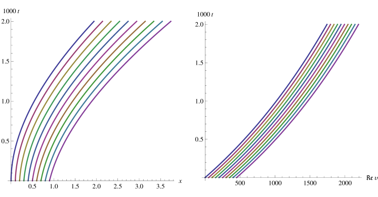
Figure 1: Example of the trajectories: The left diagram shows the trajectories $x(\xi,\tau)$, the right one the corresponding real parts of the singularities $v=\varphi(\xi,\tau)$ for incrementing values of the initial position $\mathop{\mathfrak{Re}}\xi$. The other parameters are $v_{0}=-i,~{}v_{1}=0.001,~{}\tau_{0}=0.002,~{}\omega_{p}=10^{4}$. The imaginary part of the velocity $\mathop{\mathfrak{Im}}(\xi)/\tau_{0}$ remains constant throughout the evolution.

The corresponding singularity manifold $v-\varphi(\xi,\tau)=0$ may be obtained from $\varphi=x_{\tau}$

$$\varphi(\xi,\tau)=\xi/\tau_{0}+2\pi i\omega_{p}^{2}v_{0}\tau_{0}^{2}\ln u+v_{1}$$ (17)

The acceleration due to the electric field is fading

$$a(x,\tau)=x_{\tau\tau}\bigl{(}\xi(x,t),\tau\bigr{)}=\frac{2\pi i\omega_{p}^{2}v_{0}\tau_{0}^{2}}{\tau_{0}+\tau}.$$ (18)

It is independent of $\xi$ (and consequently of $x$) which means that the electric field is spatially uniform all the time.

Finally, the residuum $F_{0}$ of the solution $F$, at the pole surface $v=\varphi(\xi,\tau)=\phi(x,t)$, is equal to $a(x,t)$, up to a constant factor

$$F_{0}(\xi,\tau)=v_{0}\tau_{0}^{2}/(\tau_{0}+\tau)$$ (19)

The singularity at $\tau=-\tau_{0}$ does not belong to the family of those solvable with respect to $v$. It is harmless if $\tau_{0}>0$ and we consider only solutions for $\mathop{\mathfrak{Re}}(\tau)>0$. The calculation is local in $\xi$ and $\tau$ and may leave $\tau=\tau_{0}$ outside the considered singularity manifold.

The solution for $F$ may be obtained on the basis of the $x_{\tau\tau}$ calculated in (18), as the acceleration is the same $a(x,t)$ for the singularity trajectory and all the other electron trajectories. By the method of characteristics we obtain in a straightforward way

$$F(x,v,t)=F\bigl{(}x\!-\!vt\!-\!2\pi i\omega_{p}^{2}\tau_{0}^{3}v_{0}\,[\ln(1\!+\!t/\tau_{0})-t/\tau_{0}],\,v\!-\!2\pi i\omega_{p}^{2}\tau_{0}^{2}v_{0}\ln(1\!+\!t/\tau_{0}),0\bigr{)},$$ (20)

assuming that the initial conditions are set out at $t=\tau=0$ (please note that the constants $x_{0}$, $\tau_{0}$ and $v_{0}$ are not the initial values of $x$, $\tau$ and $x_{\tau}$).

To comply with the assumption of the first order pole, we have to limit the initial conditions to those having a pole at $v=\varphi(x,0)$ in the upper half-plane. The physical sense of $F(x,v,t)$ requires a symmetric (complex conjugate) second pole in the lower half-plane. An example of such initial conditions could be the Cauchy distribution in $v$

$$\frac{1}{\pi}\,\frac{\gamma}{(v-v_{C})^{2}+\gamma^{2}},$$ (21)

where the center-of-mass velocity $v_{C}=0$ if the plasma as a whole is at rest, while $\pm i\gamma$ are positions of the poles. Then $\gamma=\pm\mathop{\mathfrak{Im}}(\xi/\tau_{0})$.

The initial spatial dependence of $F$ is not limited in principle, except that the integral of $F$ over velocity has to be independent of $x$, to ensure uniformity of the electric field. The physical sense of $F$ as the cumulative distribution in $x$ requires that it be a positive and non-decreasing function of $x$ for all $v$. It follows from (20) that an initially uniform (in space) distribution $F$ remains spatially uniform throughout the evolution. Thus no spontaneous breaking of the translational symmetry occurs.

Conclusions

The singularity analysis may be performed for the Vlasov equation, though the analysis is not the typical P-test.

For the one-dimensional Vlasov equation, the method provides classification of solutions which are globally meromorphic in the velocity space and free of movable branching in the position and time, except for the constant-time singularity $t=-\tau_{0}$.

The common acceleration $a(x,t)$ at a given point $x$ and moment $t$ can be calculated, provided that we find the trajectories of the poles $v={x^{j}}_{\tau^{j}}(\xi^{j},\tau^{j})$, where $\xi^{j},~{}\tau^{j}$ are the Lagrangian coordinates given by (I). Then the solution of the Vlasov equation may be obtained by the method of characteristics.

The system of equations determining the Eulerian from Lagrangian coordinates is an overdetermined system. The solutions satisfying the P-test are selected by the compatibility condition.

In case of simple poles, all the constraints are imposed on the lowest-order coefficient ${F^{j}}_{0}(\xi^{j},\tau^{j})$.

The simplest case of one simple pole in the upper complex half-plane ($\mathop{\mathfrak{Im}}{v}>0$) may easily be solved explicitly. The solution corresponds to a uniform electric field. An initially uniform solution remains uniform throughout the evolution, however the method works also for nonuniform initial distributions. In all these cases the characteristics are free from crossings, thus the initial position of the trajectory can be uniquely determined, given their actual position and time, from equation (I).

Obviously the case of the uniform electric field could have been solved without the P-test machine. However the method also works for more complex situations, with greater number of poles. The compatibility condition provides an extra equation, which restricts the class of solutions and may facilitate solving the equations. The case of more than one pole will be discussed in the next paper.

The method requires that the solution has poles in the velocity space. Therefore it does not cover the important Maxwellian distribution.

References

- (1) Bernstein, I.B., Greene, J.M., and Kruskal, M.D., Exact Nonlinear Plasma Oscillations, 1957, Phys. Rev., 108, 546–550.
- (2) Roberts, K.V. and Berk H.L. 1967, Nonlinear evolution of a two-stream instability, Phys. Rev. Lett. 19, 297–301.
- (3) Dorozhkina, D.S., and Semenov, V.E., Exact Solution of Vlasov Equations for Quasineutral Expansion of Plasma Bunch into Vacuum, Phys. Rev. Lett. 81, 2691–2694.
- (4) Klimontovich, Yu. L., 1983, The Kinetic Theory of Electromagnetic Processes, Springer New York.
- (5) Conte R. (1999) The Painlevé approach to nonlinear ordinary differential equations, chapter 3, 77–180 in The Painlevé Property One Century Later, ed. R. Conte, New York, Springer Verlag.
- (6) Conte R. and Musette M. (2008) The Painlevé Handbook, Dordrecht, Springer.
- (7) Kovalevski, S. V., 1889, Sur le problème de la rotation d’un corps solide autour d’un point fixe, Acta Math. 12, 177–232.
- (8) Ablowitz M. J., Ramani A. and Segur H. (1980) A connection between nonlinear evolution equations and ordinary differential equations of P-type J. Math. Phys. 21 715–721 and 1006–1015.
- (9) Weiss J., Tabor M. and Carnevale G., 1983, The Painlevé property for partial differential equations, J. Math. Phys. 24 522–526.
- (10) Goldstein, P.P., 1987, Testing the Painlev property of the Maxwell-Bloch and reduced Maxwell-Bloch equations, Phys. Lett. A 121, 11–14.
- (11) Infeld, E. and Rowlands, G., Lagrangian Picture of Plasma Physics, Polish Scientific Publishers PWN, Warsaw 1998, reprinted from J. Tech. Phys. 38, 607–645, and 39, 3–35.
- (12) Infeld, E. and Rowlands, G, Nonlinear Oscillations in a Warm Plasma, 1987, Phys. Rev. Lett. 58, 2063–2066; and 1988, Simple Model for the Nonlinar Evolution of the Rayleigh-Taylor Instability, Phys. Rev. Lett. 60, 2273–2275.