Distinguishing Legendrian knots with trivial orientation-preserving symmetry group

Abstract.

In a recent work of I. Dynnikov and M. Prasolov a new method of comparing Legendrian knots is proposed. In general, to apply the method requires a lot of technical work. In particular, one needs to search all rectangular diagrams of surfaces realizing certain dividing configurations. In this paper, it is shown that, in the case when the orientation-preserving symmetry group of the knot is trivial, this exhaustive search is not needed, which simplifies the procedure considerably. This allows one to distinguish Legendrian knots in certain cases when the computation of the known algebraic invariants is infeasible or not informative. In particular, it is disproved here that when $A\subset\mathbb{R}^{3}$ is an annulus tangent to the standard contact structure along $\partial A$, then the two components of $\partial A$ are always equivalent Legendrian knots. A candidate counterexample was proposed recently by I. Dynnikov and M. Prasolov, but the proof of the fact that the two components of $\partial A$ are not Legendrian equivalent was not given. Now this work is accomplished. It is also shown here that the problem of comparing two Legendrian knots having the same topological type is algorithmically solvable provided that the orientation-preserving symmetry group of these knots is trivial.

Introduction

Deciding whether or knot two Legendrian knots in $\mathbb{S}^{3}$ having the same classical invariants (see definitions below) are Legendrian isotopic is not an easy task in general. There are two major tools used for classification of Legendrian knots of a fixed topological type: Legendrian knot invariants having algebraic nature (see Chekanov [3], Eliashberg [13], Fuchs [21], Ng [35, 36], Ozsváth–Szabó–Thurston [37], Pushkar’–Chekanov [38]), and Giroux’s convex surfaces endowed with the characteristic foliation (see Eliashberg–Fraser [14, 15], Etnyre–Honda [16], Etnyre–LaFountain–Tosun [17], Etnyre–Ng–Vértesi [18], Etnyre–Vértesi [19]).

The Legendrian knot atlas by W. Chongchitmate and L. Ng [5] summarizes the classification results for Legendrian knots having arc index at most $9$. As one can see from [5] there are still many gaps in the classification even for knots with a small arc index/crossing number. Namely, there are many pairs of Legendrian knot types which are conjectured to be distinct but are not distinguished by means of the existing methods.

The works [9, 10] by I. Dynnikov and M. Prasolov propose a new combinatorial technique for dealing with Giroux’s convex surfaces. This includes a combinatorial presentation of convex surfaces in $\mathbb{S}^{3}$ and a method that allows, in certain cases, to decide whether or not a convex surface with a prescribed topological structure of the dividing set exists.

The method of [9, 10] is useful for distinguishing Legendrian knots, but it requires, in each individual case, a substantial amount of technical work and a smart choice of a Giroux’s convex surface whose boundary contains one of the knots under examination.

In the present paper we show that there is a way to make this smart choice in the case when the examined knots have no topological (orientation-preserving) symmetries, so that the remaining technical work described in [10] becomes unnecessary as the result is known in advance. This makes the procedure completely algorithmic and allows us, in particular, to distinguish two specific Legendrian knots for which computation of the known algebraic invariants is infeasible due to the large complexity of the knot presentations.

The two knots in question are of interest due to the fact that they cobound an annulus embedded in $\mathbb{S}^{3}$ and have zero relative Thurston–Bennequin and rotation invariants. They were proposed in [9] as a candidate counterexample to the claim of [27] that the two boundary components of such an annulus must be Legendrian isotopic.

The main technical result of this paper was announced by us in [11] without complete proof. In [7] the method of this paper is used to show that one can compare transverse link types in a similar fashion provided that the orientation-preserving symmetry group of the links is trivial. In a forthcoming paper by I. Dynnikov and M. Prasolov it will be shown how to drop the no symmetry assumption and to produce algorithms for comparing Legendrian and transverse link types in the general case.

The paper is organized as follows. In Section 1 we recall the definition of a Legendrian knot, and introduce the basic notation. In Section 2 we discuss annuli with Legendrian boundary whose components have zero relative Thurston–Bennequin number. In Section 3 we define the orientation-preserving symmetry group of a knot and introduce some $\mathbb{S}^{3}$-related notation. In Section 4 we recall the definition of a rectangular diagram of a knot and discuss the relation of rectangular diagrams to Legendrian knots. Section 5 discusses rectangular diagrams of surfaces. Here we describe the smart choice of a surface mentioned above (Lemma 5.1). In Section 6 we prove the triviality of the orientation-preserving symmetry group of the concrete knots that are discussed in the paper (modulo the proof of hyperbolicity of the two complicated knots cobounding an annulus but not Legendrian equivalent, which is postponed till Section 8). In Section 7 we prove a number of statements about the non-equivalence of the considered Legendrian knots.

Acknowledgement

The work is supported by the Russian Science Foundation under grant 19-11-00151.

1. Legendrian knots

All general statements about knots in this paper can be extended to many-component links. To simplify the exposition, we omit the corresponding formulations, which are pretty obvious but sometimes slightly more complicated.

All knots in this paper are assumed to be oriented. The knot obtained from a knot $K$ by reversing the orientation is denoted by $-K$.

Definition 1.1.

Let $\xi$ be a contact structure in the three-space $\mathbb{R}^{3}$, that is, a smooth $2$-plane distribution that locally has the form $\ker\alpha$, where $\alpha$ is a differential $1$-form such that $\alpha\wedge d\alpha$ does not vanish. A smooth curve $\gamma$ in $\mathbb{R}^{3}$ is called $\xi$-Legendrian if it is tangent to $\xi$ at every point $p\in\gamma$.

A $\xi$-Legendrian knot is a knot in $\mathbb{R}^{3}$ which is a $\xi$-Legendrian curve. Two $\xi$-Legendrian knots $K$ and $K^{\prime}$ are said to be equivalent if there is a diffeomorphism $\varphi:\mathbb{R}^{3}\rightarrow\mathbb{R}^{3}$ preserving $\xi$ such that $\varphi(K)=K^{\prime}$ (this is equivalent to saying that there is an isotopy from $K$ to $K^{\prime}$ through Legendrian knots).

The contact structure $\xi_{+}=\ker(x\,dy+dz)$, where $x,y,z$ are the coordinates in $\mathbb{R}^{3}$, will be referred to as the standard contact structure. If $\xi=\xi_{+}$ we often abbreviate ‘$\xi$-Legendrian’ to ‘Legendrian’.

In this paper we also deal with the following contact structure, which is a mirror image of $\xi_{+}$:

$$\xi_{-}=\ker(x\,dy-dz).$$

We denote by $r_{-},r_{\medvert}:\mathbb{R}^{3}\rightarrow\mathbb{R}^{3}$ the orthogonal reflections in the $xy$- and $xz$-planes, respectively: $r_{-}(x,y,z)=(x,y,-z)$, $r_{\medvert}(x,y,z)=(x,-y,z)$. Clearly, if $K$ is a $\xi_{+}$-Legendrian knot, then $r_{-}(K)$ and $r_{\medvert}(K)$ are $\xi_{-}$-Legendrian knots, and vice versa. It is also clear that the contact structures $\xi_{+}$ and $\xi_{-}$ are invariant under the transformation $r_{-}\circ r_{\medvert}:(x,y,z)\mapsto(x,-y,-z)$ (however, if the contact structures are endowed with an orientation, then the latter is flipped).

It is well known that a Legendrian knot in $\mathbb{R}^{3}$ is uniquely recovered from its front projection, which is defined as the projection to the $yz$-plane along the $x$-axis, provided that this projection is generic (a projection is generic if it has only finitely many cusps and only double self-intersections, which are also required to be disjoint from cusps). Note that a front projection always has cusps, since the tangent line to the projection cannot be parallel to the $z$-axis. Note also that at every double point of the projection the arc having smaller slope $dz/dy$ is overpassing.

An example of a generic front projection is shown in Figure 1.

Figure 1. Front projection of a Legendrian knot

There are two well known integer invariants of Legendrian knots called Thurston–Bennequin number and rotation number. We recall their definitions.

Definition 1.2.

The Thurston–Bennequin number $\mathop{tb}\nolimits(K)$ of a Legendrian knot $K$ having generic front projection is defined as

$$\mathop{tb}\nolimits(K)=w(K)-c(K)/2,$$

where $w(K)$ is the writhe of the projection (that is, the algebraic number of double points), and $c(K)$ is the total number of cusps of the projection.

Definition 1.3.

A cusp of a front projection is said to be oriented up if the outgoing arc appears above the incoming one, and oriented down otherwise (see Figure 2).

oriented up		oriented down

Figure 2. Cusps oriented up and down

The rotation number $r(K)$ of a Legendrian knot $K$ having generic front projection is defined as

$$r(K)=(c_{\mathrm{down}}(K)-c_{\mathrm{up}}(K))/2,$$

where $c_{\mathrm{down}}(K)$ (respectively, $c_{\mathrm{up}}(K)$) is the number of cusps of the front projection of $K$ oriented down (respectively, up).

For instance, if $K$ is the Legendrian knot shown in Figure 1, then $\mathop{tb}\nolimits(K)=-10$, $r(K)=1$.

The topological meaning of $\mathop{tb}\nolimits$ and $r$ is as follows. Let $v$ be a normal vector field to $\xi$. Then $\mathop{tb}\nolimits(K)$ is the linking number $\mathop{lk}\nolimits(K,K^{\prime})$, where $K^{\prime}$ is obtained from $K$ by a small shift along $v$. The rotation number $r(K)$ is equal to the degree of the map $K\rightarrow\mathbb{S}^{1}$ defined in a local parametrization $(x(t),y(t),z(t))$ of $K$ by $(x,y,z)\mapsto(\dot{x},\dot{y})/\sqrt{\dot{x}^{2}+\dot{y}^{2}}$.

If $K$ is a Legendrian knot, then by the classical invariants of $K$ one means the topological type of $K$ together with $\mathop{tb}\nolimits(K)$ and $r(K)$.

Sometimes the classical invariants determine the equivalence class of a Legendrian knot completely (in which case the knot is said to be Legendrian simple). This occurs, for instance, when $K$ is an unknot [14, 15], a figure eight knot, or a torus knot [16]. But many examples of Legendrian non-simple knots are known.

Definition 1.4.

Let $K$, $K^{\prime}$ be Legendrian knots. We say that $K^{\prime}$ is obtained from $K$ by a positive stabilization (respectively, negative stabilization), and $K$ is obtained from $K^{\prime}$ by a positive destabilization (respectively, negative destabilization), if there are Legendrian knots $K^{\prime\prime}$, $K^{\prime\prime\prime}$ equivalent to $K$ and $K^{\prime}$, respectively, such that the front projection of $K^{\prime\prime\prime}$ is obtained from the front projection of $K^{\prime\prime}$ by a local modification shown in Figure 3(a) (respectively, Figure 3(b)).

(a)		(b)

Figure 3. Stabilizations and destabilizations of Legendrian knots: (a) positive; (b) negative

A positive (respectively, negative) stabilization shifts the $(\mathop{tb}\nolimits,r)$ pair of the Legendrian knot by $(-1,1)$ (respectively, by $(-1,-1)$), so stabilizations and destabilizations always change the equivalence class of a Legendrian knot. If $K$ is a Legendrian knot we denote by $S_{+}(K)$ (respectively, $S_{-}(K)$) the result of a positive (respectively, negative) stabilization applied to $K$.

One can see that the equivalence class of the Legendrian knot $S_{+}(K)$ is well defined. If $\mathscr{L}$ is an equivalence class of Legendrian knots, then by $S_{+}(\mathscr{L})$ (respectively, $S_{-}(\mathscr{L})$) we denote the class $\{S_{+}(K):K\in\mathscr{L}\}$ (respectively, $\{S_{-}(K):K\in\mathscr{L}\}$).

Remark 1.1.

In the case of links having more than one component, the result of a stabilization, viewed up to Legendrian equivalence, depends on which component of the link the modification shown in Figure 3 is applied to, so the notation should be refined accordingly.

As shown in [20] any two Legendrian knots that have the same topological type can be obtained from one another by a sequence of stabilizations and destabilizations.

Definition 1.5.

If $K$ is a $\xi_{+}$-Legendrian or $\xi_{-}$-Legendrian knot then the image of $K$ under the transformation $r_{-}\circ r_{\medvert}$ is called the Legendrian mirror of $K$ and denoted by $\mu(K)$.

Note that in terms of the respective front projections Legendrian mirroring is just a rotation by $\pi$ around the origin. It preserves the Thurston–Bennequin number of the knot and reverses the sign of its rotation number. Thus, if $K$ is a Legendrian knot with $r(K)=0$, then $K$ and $\mu(K)$ have the same classical invariants. However, it happens pretty often in this case that $\mu(K)$ and $K$ are not equivalent Legendrian knots (see examples in Section 7).

Similarly, if $K$ is a Legendrian knot whose topological type is invertible, then $-\mu(K)$ and $K$ have the same classical invariants, but may not be equivalent Legendrian knots.

Definition 1.6.

If $K$ is a $\xi_{-}$-Legendrian knot, the Thurston–Bennequin and rotation numbers of $K$, as well as positive and negative stabilizations, are defined by using the mirror image $r_{\medvert}(K)$ as follows:

$$\mathop{tb}\nolimits(K)=\mathop{tb}\nolimits(r_{\medvert}(K)),\quad r(K)=r(r_{\medvert}(K)),\quad S_{+}(K)=r_{\medvert}\bigl{(}S_{+}(r_{\medvert}(K))\bigr{)},\quad S_{-}(K)=r_{\medvert}\bigl{(}S_{-}(r_{\medvert}(K))\bigr{)}.$$

2. Annuli

Definition 2.1.

Let $K$ be a Legendrian knot, and let $F$ be an oriented compact surface embedded in $\mathbb{R}^{3}$ such that $K\subset\partial F$ and the orientation of $K$ agrees with the induced orientation of $\partial F$. Let also $v$ be a normal vector field to $\xi_{+}$. By the Thurston–Bennequin number of $K$ relative to $F$ denoted $\mathop{tb}\nolimits(K;F)$ we call the intersection index of $F$ with a knot obtained from $K$ by a small shift along $v$.

If $F$ is an arbitrary compact surface embedded in $\mathbb{R}^{3}$ such that $K\subset\partial F$, then $\mathop{tb}\nolimits(K;F)$ is defined as $\mathop{tb}\nolimits(K;F^{\prime})$, where $F^{\prime}$ is the appropriately oriented intersection of a small tubular neighborhood $U$ of $K$ with $F$ (the shift of $K$ along $v$ should then be chosen so small that the shifted knot does not escape from $U$).

Let $K$ be a Legendrian knot, and let $F\subset\mathbb{R}^{3}$ be a compact surface such that $K\subset\partial F$. It is elementary to see that the following three conditions are equivalent:

1. $\mathop{tb}\nolimits(K;F)=0$;

2. $F$ is isotopic relative to $K$ to a surface $F^{\prime}$ such that $F^{\prime}$ is tangent to $\xi_{+}$ along $K$;

3. $F$ is isotopic relative to $K$ to a surface $F^{\prime}$ such that $F^{\prime}$ is transverse to $\xi_{+}$ along $K$.

In 3-dimensional contact topology, Giroux’s convex surfaces play a fundamental role [24, 25, 26]. Especially important are convex annuli with Legendrian boundary and relative Thurston–Bennequin numbers of both boundary component equal to zero, since, vaguely speaking, any closed convex surface, viewed up to isotopy in the class of convex surfaces, can be build up from such annuli by gluing along a Legendrian graph.

Let $A\subset\mathbb{R}^{3}$ be an annulus with boundary consisting of two Legendrian knots $K_{1}$ and $K_{2}$ such that $\mathop{tb}\nolimits(K_{1};A)=\mathop{tb}\nolimits(K_{2};A)=0$, $\partial A=K_{1}\cup(-K_{2})$. Then the knots $K_{1}$ and $K_{2}$ have the same classical invariants, and it is natural to ask whether they must always be equivalent as Legendrian knots.

A quick look at this problem reveals no obvious reason why $K_{1}$ and $K_{2}$ must be equivalent, but constructing a counterexample appears to be tricky.

Theorem 8.1 of [27], which is given without a complete proof, implies that $K_{1}$ and $K_{2}$ are always equivalent Legendrian knots even in a more general situation in which $\mathbb{R}^{3}$ is replaced by an arbitrary tight contact $3$-manifold.

However, counterexamples to this more general claim appeared earlier in a work of P. Ghiggini [23] (without a special emphasis on the phenomenon), the simplest of which is as follows. Endow the three-dimensional torus $\mathbb{T}^{3}=(\mathbb{R}/\mathbb{Z})^{3}$ with the contact structure $\xi=\ker\bigl{(}\sin(2\pi z)\,dx+\cos(2\pi z)\,dy\bigr{)}$, and take for $A$ the annulus $(\mathbb{R}/\mathbb{Z})\times\{0\}\times[0;1/2]$. This annulus is clearly tangent to $\xi$ along $\partial A$, but the boundary components are not Legendrian isotopic according to [23, Proposition 7.1] (the fact that $(\mathbb{T}^{3},\xi)$ is a tight contact manifold was established earlier by E. Giroux).

In this example, and in similar ones from [23], any connected component of $\partial A$ can be taken to the other by a contactomorphism of $(\mathbb{T}^{3},\xi)$. So, it is important here that the group of contactomorphisms of $(\mathbb{T}^{3},\xi)$ is disconnected, which is not the case for the standard contact structure on $\mathbb{R}^{3}$. Another feature of this example is that the boundary components of $A$ are not null-homologous.

The following statement shows that the assertion of [27, Theorem 8.1] is false in the case of $\mathbb{R}^{3}$, too.

Theorem 2.1.

There exists an oriented annulus $A\subset\mathbb{R}^{3}$ with boundary $\partial A=K_{1}\cup(-K_{2})$ such that $K_{1}$ and $K_{2}$ are nonequivalent Legendrian knots having zero Thurston–Bennequin number relative to $A$.

The proof is by producing an explicit example, and the example we use here is proposed by I. Dynnikov and M. Prasolov in [9]. Front projections of the Legendrian knots from this example are shown in Figure 4. It is shown in [9] that they cobound an embedded annulus such that $\mathop{tb}\nolimits(K_{1};A)=\mathop{tb}\nolimits(K_{2};A)=0$, and it has been remaining unproved that $K_{1}$ and $K_{2}$ are not Legendrian equivalent.

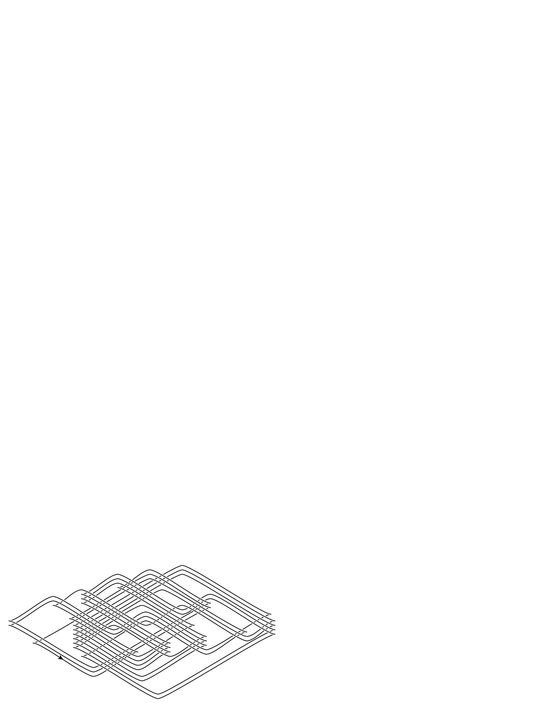
Figure 4. Nonequivalent Legendrian knots $K_{1}$ and $K_{2}$ cobounding an annulus $A$ such that $\mathop{tb}\nolimits(K_{1};A)=\mathop{tb}\nolimits(K_{2};A)=0$, $\partial A=K_{1}\cup(-K_{2})$

The proof of Theorem 2.1 is given in Section 7.

3. $\mathbb{S}^{3}$ settings. The orientation-preserving symmetry group

By $\mathbb{S}^{3}$ we denote the unit $3$-sphere in $\mathbb{R}^{4}$, which we identify with the group $SU(2)$ in the standard way. We use the following parametrization of this group:

$$(\theta,\varphi,\tau)\mapsto\begin{pmatrix}\cos(\pi\tau/2)e^{\mathbbm{i}\varphi}&\sin(\pi\tau/2)e^{\mathbbm{i}\theta}\\ -\sin(\pi\tau/2)e^{-\mathbbm{i}\theta}&\cos(\pi\tau/2)e^{-\mathbbm{i}\varphi}\end{pmatrix},$$

where $(\theta,\varphi,\tau)\in(\mathbb{R}/(2\pi\mathbb{Z}))\times(\mathbb{R}/(2\pi\mathbb{Z}))\times[0;1]$. The coordinate system $(\theta,\varphi,\tau)$ can also be viewed as the one coming from the join construction $\mathbb{S}^{3}\cong\mathbb{S}^{1}*\mathbb{S}^{1}$, with $\theta$ the coordinate on $\mathbb{S}^{1}_{\tau=1}$, and $\varphi$ on $\mathbb{S}^{1}_{\tau=0}$. Let $\alpha_{+}$ be the following right-invariant $1$-form on $\mathbb{S}^{3}\cong SU(2)$:

$$\alpha_{+}(X)=\frac{1}{2}\mathop{tr}\nolimits\left(X^{-1}\begin{pmatrix}\mathbbm{i}&0\\ 0&-\mathbbm{i}\end{pmatrix}dX\right)=\sin^{2}\Bigl{(}\frac{\pi\tau}{2}\Bigr{)}\,d\theta+\cos^{2}\Bigl{(}\frac{\pi\tau}{2}\Bigr{)}\,d\varphi.$$

It is known (see [22]) that, for any point $p\in\mathbb{S}^{3}$, there is a diffeomorphism $\phi$ from $\mathbb{R}^{3}$ to $\mathbb{S}^{3}\setminus\{p\}$ that takes the contact structure $\xi_{+}$ to the one defined by $\alpha_{+}$, that is, to $\ker\alpha_{+}$. For this reason, the latter is denoted by $\xi_{+}$, too. Two Legendrian knots in $\mathbb{R}^{3}$ are equivalent if and only if so are their images under $\phi$ in $\mathbb{S}^{3}$. We will switch between the $\mathbb{R}^{3}$ and $\mathbb{S}^{3}$ settings depending on which is more suitable in the current context. The $\mathbb{R}^{3}$ settings are usually more visual, but sometimes are not appropriate. In particular, the definition of the knot symmetry group given below requires the $\mathbb{S}^{3}$ settings.

Definition 3.1.

Let $K$ be a smooth knot in $\mathbb{S}^{3}$. Denote by $\mathrm{Diff}^{*}(\mathbb{S}^{3};K)$ the group of diffeomorphisms of $\mathbb{S}^{3}$ preserving the orientation of $\mathbb{S}^{3}$ and the orientation of $K$, and by $\mathrm{Diff}^{*}_{0}(\mathbb{S}^{3};K)$ the connected component of this group containing the identity. The group $\mathrm{Diff}^{*}(\mathbb{S}^{3};K)/\mathrm{Diff}^{*}_{0}(\mathbb{S}^{3};K)$ is called the orientation-preserving symmetry group of $K$ and denoted $\mathrm{Sym^{*}}(K)$.

Clearly the group $\mathrm{Sym^{*}}(K)$ depends only on the topological type of $K$. In this paper we are dealing with knots $K$ for which $\mathrm{Sym^{*}}(K)$ is a trivial group.

In the $\mathbb{S}^{3}$ settings, we also define the mirror image $\xi_{-}$ of $\xi_{+}$ as

$$\xi_{-}=\ker\left(\sin^{2}\Bigl{(}\frac{\pi\tau}{2}\Bigr{)}\,d\theta-\cos^{2}\Bigl{(}\frac{\pi\tau}{2}\Bigr{)}\,d\varphi\right).$$

4. Rectangular diagrams of knots

We denote by $\mathbb{T}^{2}$ the two-dimensional torus $\mathbb{S}^{1}\times\mathbb{S}^{1}$, and by $\theta$ and $\varphi$ the angular coordinates on the first and the second $\mathbb{S}^{1}$ factor, respectively.

Definition 4.1.

An oriented rectangular diagram of a link is a finite subset $R\subset\mathbb{T}^{2}$ with an assignment ‘$+$’ or ‘$-$’ to every point in $R$ such that every meridian $\{\theta\}\times\mathbb{S}^{1}$ and every longitude $\mathbb{S}^{1}\times\{\varphi\}$ contains either no or exactly two points from $R$, and in the latter case one of the points is assigned ‘$+$’ and the other ‘$-$’. The points in $R$ are called vertices of $R$, and the pairs $\{u,v\}\subset R$ such that $\theta(u)=\theta(v)$ (respectively, $\varphi(u)=\varphi(v)$) are called vertical edges (respectively, horizontal edges) of $R$.

A rectangular diagram of a link is defined similarly, without assignment ‘$+$’ or ‘$-$’ to vertices.

An (oriented) rectangular diagram $R$ of a link is called an (oriented) rectangular diagram of a knot if it is connected in the sense that, for any two vertices $v,v^{\prime}\in R$, there exists a sequence $v_{0}=v,v_{1},v_{2},\ldots,v_{k}=v^{\prime}$ of vertices of $R$ such that any pair $v_{i-1},v_{i}$ of successive elements in it is an edge of $R$.

From the combinatorial point of view, oriented rectangular diagrams of links are the same thing as grid diagrams [32] viewed up to cyclic permutations of rows and columns. They are also nearly the same thing as arc-presentations (see [6]).

Convention.

In this paper we mostly work with oriented knots and knot diagrams. For brevity, unless a rectangular diagram is explicitly specified as unoriented it is assumed to be oriented.

With every rectangular diagram of a knot $R$ one associates a knot, denoted $\widehat{R}$, in $\mathbb{S}^{3}$ as follows. For a vertex $v\in R$ denote by $\widehat{v}$ the image of the arc $v\times[0;1]$ in $\mathbb{S}^{3}\cong\mathbb{S}^{1}*\mathbb{S}^{1}=(\mathbb{T}^{2}\times[0;1])/{\sim}$ oriented from $0$ to $1$ if $v$ is assigned ‘$+$’, and from $1$ to $0$ otherwise. The knot $\widehat{R}$ is by definition $\bigcup_{v\in V}\widehat{v}$.

To get a planar diagram of a knot in $\mathbb{R}^{3}$ equivalent to $\widehat{R}$ one can proceed a follows. Cut the torus $\mathbb{T}^{2}$ along a meridian and a longitude not passing through a vertex of $R$ to get a square. For every edge $\{u,v\}$ of $R$ join $u$ and $v$ by a straight line segment, and let vertical segments overpass horizontal ones at every crossing point. Vertical edges are oriented from ‘$+$’ to ‘$-$’, and the horizontal ones from ‘$-$’ to ‘$+$’, see Figure 5.

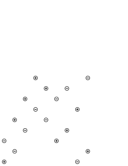
Figure 5. A rectangular diagram of a knot and the corresponding planar diagram

One can show (see [6]) that the obtained planar diagram represents a knot equivalent to $\widehat{R}$.

For two distinct points $x,y\in\mathbb{S}^{1}$ we denote by $[x;y]$ the arc of $\mathbb{S}^{1}$ such that, with respect to the standard orientation of $\mathbb{S}^{1}$, it has the starting point at $x$, and the end point at $y$.

Definition 4.2.

Let $R_{1}$ and $R_{2}$ be rectangular diagrams of a knot such that, for some $\theta_{1},\theta_{2},\varphi_{1},\varphi_{2}\in\mathbb{S}^{1}$, the following holds:

1. $\theta_{1}\neq\theta_{2}$, $\varphi_{1}\neq\varphi_{2}$;

2. the symmetric difference $R_{1}\triangle R_{2}$ is $\{\theta_{1},\theta_{2}\}\times\{\varphi_{1},\varphi_{2}\}$;

3. $R_{1}\triangle R_{2}$ contains an edge of one of the diagrams $R_{1}$, $R_{2}$;

4. none of $R_{1}$ and $R_{2}$ is a subset of the other;

5. the intersection of the rectangle $[\theta_{1};\theta_{2}]\times[\varphi_{1};\varphi_{2}]$ with $R_{1}\cup R_{2}$ consists of its vertices, that is, $\{\theta_{1},\theta_{2}\}\times\{\varphi_{1},\varphi_{2}\}$;

6. each $v\in R_{1}\cap R_{2}$ is assigned the same sign in $R_{1}$ as in $R_{2}$.

Then we say that the passage $R_{1}\mapsto R_{2}$ is an elementary move.

An elementary move $R_{1}\mapsto R_{2}$ is called:

• an exchange move if $|R_{1}|=|R_{2}|$,

• a stabilization move if $|R_{2}|=|R_{1}|+2$, and

• a destabilization move if $|R_{2}|=|R_{1}|-2$,

where $|R|$ denotes the number of vertices of $R$.

We distinguish two types and four oriented types of stabilizations and destabilizations as follows.

Definition 4.3.

Let $R_{1}\mapsto R_{2}$ be a stabilization, and let $\theta_{1},\theta_{2},\varphi_{1},\varphi_{2}$ be as in Definition 4.2. Denote by $V$ the set of vertices of the rectangle $[\theta_{1};\theta_{2}]\times[\varphi_{1};\varphi_{2}]$. We say that the stabilization $R_{1}\mapsto R_{2}$ and the destabilization $R_{2}\mapsto R_{1}$ are of type I (respectively, of type II) if $R_{1}\cap V\in\{(\theta_{1},\varphi_{1}),(\theta_{2},\varphi_{2})\}$ (respectively, $R_{1}\cap V\in\{(\theta_{1},\varphi_{2}),(\theta_{2},\varphi_{1})\}$).

Let $\varphi_{0}\in\{\varphi_{1},\varphi_{2}\}$ be such that $\{\theta_{1},\theta_{2}\}\times\{\varphi_{0}\}\subset R_{2}$. The stabilization $R_{1}\mapsto R_{2}$ and the destabilization $R_{2}\mapsto R_{1}$ are of oriented type $\overrightarrow{\mathrm{I}}$ (respectively, of oriented type $\overrightarrow{\mathrm{II}}$) if they are of type I (respectively, of type II) and $(\theta_{2},\varphi_{0})$ is a positive vertex of $R_{2}$. The stabilization $R_{1}\mapsto R_{2}$ and the destabilization $R_{2}\mapsto R_{1}$ are of oriented type $\overleftarrow{\mathrm{I}}$ (respectively, of oriented type $\overleftarrow{\mathrm{II}}$) if they are of type I (respectively, of type II) and $(\theta_{2},\varphi_{0})$ is a negative vertex of $R_{2}$.

Our notation for stabilization types follows [8]. The correspondence with the notation of [37] is as follows:

notation of [8] $\overrightarrow{\mathrm{I}}$ $\overleftarrow{\mathrm{I}}$ $\overrightarrow{\mathrm{II}}$ $\overleftarrow{\mathrm{II}}$ notation of [37] X:NE, O:SW X:SW, O:NE X:SE, O:NW X:NW, O:SE

With every rectangular diagram of a knot $R$ we associate an equivalence class $\mathscr{L}_{+}(R)$ of $\xi_{+}$-Legendrian knots and an equivalence class $\mathscr{L}_{-}(R)$ of $\xi_{-}$-Legendrian knots as follows. The front projection of a representative of $\mathscr{L}_{+}(R)$ (respectively, of $\mathscr{L}_{-}(R)$) is obtained from $R$ in the following three steps: (1) produce a conventional planar diagram from $R$ as described above; (2) rotate it counterclockwise (respectively, clockwise) by any angle between $0$ and $\pi/2$; (3) smooth out. See Figure 6 for an example.

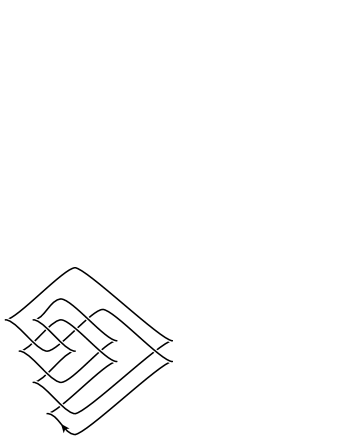
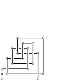
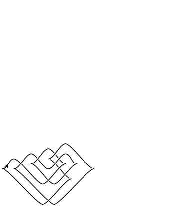
a representative of $\mathscr{L}_{+}(R)$		$R$		a representative of $\mathscr{L}_{-}(R)$

Figure 6. Legendrian knots associated with a rectangular diagram of a knot

Theorem 4.1 ([37]).

Let $R_{1}$ and $R_{2}$ be rectangular diagrams of a knot. The classes $\mathscr{L}_{+}(R_{1})$ and $\mathscr{L}_{+}(R_{2})$ (respectively, $\mathscr{L}_{-}(R_{1})$ and $\mathscr{L}_{-}(R_{2})$) coincide if and only if the diagrams $R_{1}$ and $R_{2}$ are related by a finite sequence of elementary moves in which all stabilizations and destabilizations are of type I (respectively, of type II).

Moreover, if $R_{1}\mapsto R_{2}$ is a stabilization of oriented type $T$, then

$$\mathscr{L}_{-}(R_{2})=\left\{\begin{aligned} S_{-}(\mathscr{L}_{-}(R_{1})),\quad&\text{if }T=\overleftarrow{\mathrm{I}},\\ S_{+}(\mathscr{L}_{-}(R_{1})),\quad&\text{if }T=\overrightarrow{\mathrm{I}},\end{aligned}\right.\hskip 28.45274pt\mathscr{L}_{+}(R_{2})=\left\{\begin{aligned} S_{+}(\mathscr{L}_{+}(R_{1})),\quad&\text{if }T=\overleftarrow{\mathrm{II}},\\ S_{-}(\mathscr{L}_{+}(R_{1})),\quad&\text{if }T=\overrightarrow{\mathrm{II}}.\end{aligned}\right.$$

The following is the key result of the present work.

Theorem 4.2.

Let $K$ be a knot with trivial orientation-preserving symmetry group, and let $R_{1}$ and $R_{2}$ be rectangular diagrams of knots isotopic to $K$. Then the following two conditions are equivalent:

1. we have $\mathscr{L}_{+}(R_{1})=\mathscr{L}_{+}(R_{2})$ and $\mathscr{L}_{-}(R_{1})=\mathscr{L}_{-}(R_{2})$;

2. the diagram $R_{2}$ can be obtained from $R_{1}$ by a sequence of exchange moves.

The proof is given in the next section.

5. Rectangular diagrams of surfaces

Here we recall some definitions from [9, 10].

By a rectangle we mean a subset $r\subset\mathbb{T}^{2}$ of the form $[\theta_{1};\theta_{2}]\times[\varphi_{1};\varphi_{2}]$. Two rectangles $r_{1}$, $r_{2}$ are said to be compatible if their intersection satisfies one of the following:

1. $r_{1}\cap r_{2}$ is empty;

2. $r_{1}\cap r_{2}$ is a subset of vertices of $r_{1}$ (equivalently: of $r_{2}$);

3. $r_{1}\cap r_{2}$ is a rectangle disjoint from the vertices of both rectangles $r_{1}$ and $r_{2}$.

Definition 5.1.

A rectangular diagram of a surface is a collection $\Pi=\{r_{1},\ldots,r_{k}\}$ of pairwise compatible rectangles in $\mathbb{T}^{2}$ such that every meridian $\{\theta\}\times\mathbb{S}^{1}$ and every longitude $\mathbb{S}^{1}\times\{\varphi\}$ of the torus contains at most two free vertices, where by a free vertex we mean a point that is a vertex of exactly one rectangle in $\Pi$.

The set of all free vertices of $\Pi$ is called the boundary of $\Pi$ and denoted by $\partial\Pi$.

One can see that the boundary of a rectangular diagram of a surface is an unoriented rectangular diagram of a link. In particular, for any rectangle $r$, the boundary of $\{r\}$ is the set of vertices of $r$, and $\widehat{\partial\{r\}}$ is an unknot.

With every rectangular diagram of a surface $\Pi$ one associates a $C^{1}$-smooth surface $\widehat{\Pi}\subset\mathbb{S}^{3}$ with piecewise smooth boundary, as we now describe.

By the torus projection we mean the map $\mathfrak{t}:\mathbb{S}^{3}\setminus\bigl{(}\mathbb{S}^{1}_{\tau=1}\cup\mathbb{S}^{1}_{\tau=0}\bigr{)}\rightarrow\mathbb{T}^{2}$ defined by $(\theta,\varphi,\tau)\mapsto(\theta,\varphi)$. With every rectangle $r\subset\mathbb{T}^{2}$ one can associate a disc $\widehat{r}\subset\mathbb{S}^{3}$ having the form of a curved quadrilateral contained in $\overline{\mathfrak{t}^{-1}(r)}$ and spanning the loop $\widehat{\partial\{r\}}$ so that the following conditions hold:

1. for each rectangle $r$, the restriction of $\mathfrak{t}$ to the interior of $\widehat{r}$ is a one-to-one map onto the interior or $r$;

2. if $r_{1}$ and $r_{2}$ are compatible rectangles, then the interiors of $\widehat{r}_{1}$ and $\widehat{r}_{2}$ are disjoint;

3. if $r=[\theta_{1};\theta_{2}]\times[\varphi_{1};\varphi_{2}]$, then $\widehat{r}$ is tangent to $\xi_{+}$ along the sides $\widehat{(\theta_{1},\varphi_{2})}$ and $\widehat{(\theta_{2},\varphi_{1})}$, and to $\xi_{-}$ along the sides $\widehat{(\theta_{1},\varphi_{1})}$ and $\widehat{(\theta_{2},\varphi_{2})}$.

An explicit way to define the discs $\widehat{r}$, which are referred to as tiles, is given in [9, Subsection 2.3].

The surface $\widehat{\Pi}$ associated with a rectangular diagram of a surface $\Pi$ is then defined as

$$\widehat{\Pi}=\bigcup_{r\in\Pi}\widehat{r}.$$

One can show that we have $\partial\widehat{\Pi}=\widehat{\partial\Pi}$ and, for any connected component $R$ of $\partial\Pi$, the relative Thurston–Bennequin number $\mathop{tb}\nolimits_{+}(\widehat{R};\widehat{\Pi})$ (respectively, $\mathop{tb}\nolimits_{-}(\widehat{R};\widehat{\Pi})$) equals minus half the number of vertices of $R$ which are bottom-right or top-left (respectively, bottom-left or top-right) vertices of some rectangles of $\Pi$.

On every rectangular diagram of a surface $\Pi$ we introduce two binary relations, $\udotdot$ and $\ddotdot$, that keep the information about which vertices are shared between two rectangles from $\Pi$. Namely, if $r_{1},r_{2}\in\Pi$, then $r_{1}\udotdot r_{2}$ means that $r_{1}$ and $r_{2}$ have the form

$$r_{1}=[\theta_{1};\theta_{2}]\times[\varphi_{1};\varphi_{2}],\quad r_{2}=[\theta_{2};\theta_{3}]\times[\varphi_{2};\varphi_{3}],$$

and $r_{1}\ddotdot r_{2}$ means that $r_{1}$ and $r_{2}$ have the form

$$r_{1}=[\theta_{1};\theta_{2}]\times[\varphi_{2};\varphi_{3}],\quad r_{2}=[\theta_{2};\theta_{3}]\times[\varphi_{1};\varphi_{2}].$$

Proposition 5.1.

Let $R_{1}$ and $R_{2}$ be rectangular diagrams of a knot such that the knots $\widehat{R}_{1}$ and $\widehat{R}_{2}$ are topologically equivalent and have trivial orientation-preserving symmetry group. Suppose that $\mathscr{L}_{+}(R_{1})=\mathscr{L}_{+}(R_{2})$ and $\mathscr{L}_{-}(R_{1})=\mathscr{L}_{-}(R_{2})$.

Then, for any rectangular diagram of a surface $\Pi=\{r_{1},\ldots,r_{m}\}$ such that $R_{1}\subset\partial\Pi$, there exists a rectangular diagram of a surface $\Pi^{\prime}=\{r_{1}^{\prime},\ldots,r_{m}^{\prime}\}$ and a rectangular diagram of a knot $R_{2}^{\prime}$ such that:

1. $R_{2}$ and $R_{2}^{\prime}$ are related by a sequence of exchange moves;

2. there exists an orientation preserving self-homeomorphism of $\mathbb{S}^{3}$ that takes $\widehat{R}_{1}$ to $\widehat{R}_{2}^{\prime}$, and $\widehat{r}_{i}$ to $\widehat{r}_{i}^{\prime}$, $i=1,\ldots,m$;

3. $r_{i}\udotdot r_{j}\Leftrightarrow r_{i}^{\prime}\udotdot r_{j}^{\prime}$, $r_{i}\ddotdot r_{j}\Leftrightarrow r_{i}^{\prime}\ddotdot r_{j}^{\prime}$.

Proof.

This statement is a consequence of the results of [10, Section 2], namely, of Theorems 2.1 and 2.2, as we will now see. The reader is referred to [10, Section 2] for the terminology that we use here.

Denote by $D=(\delta_{+},\delta_{-})$ a canonic dividing configuration of $\widehat{\Pi}$. By hypothesis we have $\mathop{tb}\nolimits_{+}(R_{1})=\mathop{tb}\nolimits_{+}(R_{2})$ and $\mathop{tb}\nolimits_{-}(R_{1})=\mathop{tb}\nolimits_{-}(R_{2})$, which implies that $\widehat{\Pi}$ is both $+$-compatible and $-$-compatible with $R_{2}$. By [10, Theorem 2.1] there exist a proper $+$-realization $(\Pi_{+},\phi_{+})$ of $\delta_{+}$ and a proper $-$-realization $(\Pi_{-},\phi_{-})$ of $\delta_{-}$ at $R_{2}$.

Since the orientation-preserving symmetry group of $\widehat{R}_{2}$ is trivial there is an isotopy from $\phi_{+}$ to $\phi_{-}$ preserving $\widehat{R}_{2}$. One can clearly find a $-$-realization $(\Pi_{-},\phi_{-}^{\prime})$ at $R_{2}$ of an abstract dividing set equivalent to $\delta_{-}$ such that there be an isotopy from $\phi_{+}$ to $\phi_{-}^{\prime}$ that fixes $\widehat{R}_{2}$ pointwise.

By [10, Theorem 2.2] this implies the existence of a proper realization $(\Pi^{\prime},\phi)$ of $D$ and a rectangular diagram of a knot $R_{2}^{\prime}$ obtained from $R_{2}$ by a sequence of exchange moves, and such that $\phi(\widehat{R}_{1})=\widehat{R}_{2}^{\prime}$, which is just a reformulation of the assertion of Proposition 5.1. ∎

Definition 5.2.

Two rectangular diagrams of a surface (or of a knot) are said to be combinatorially equivalent if one can be taken to the other by a homeomorphism $\mathbb{T}^{2}\rightarrow\mathbb{T}^{2}\cong\mathbb{S}^{1}\times\mathbb{S}^{1}$ of the form $f\times g$, where $f$ and $g$ are orientation preserving homeomorphisms of the circle $\mathbb{S}^{1}$.

Let $\Pi$ be a rectangular diagram of a surface. The relations $\udotdot$ and $\ddotdot$ on $\Pi$ defined above constitute what is called in [10] the (equivalence class of a) dividing code of $\Pi$. In other words, two diagrams $\Pi_{1}$ and $\Pi_{2}$ have equivalent dividing codes if there is a bijection $\Pi_{1}\rightarrow\Pi_{2}$ that preserves the relations $\udotdot$ and $\ddotdot$. In general, this does not imply that the diagrams $\Pi_{1}$ and $\Pi_{2}$ are combinatorially equivalent (see [10, Figure 2.2] for an example).

Lemma 5.1.

For any rectangular diagram of a link $R$, there exists a rectangular diagram of a surface $\Pi$ such that the following holds:

1. $R\subset\partial\Pi$;

2. whenever a rectangular diagram of a surface $\Pi^{\prime}$ has the same dividing code as $\Pi$ has, the diagrams $\Pi$ and $\Pi^{\prime}$ are combinatorially equivalent.

Proof.

For simplicity we assume that $R$ is connected. In the case of a many-component link the proof is essentially the same, but a cosmetic change of notation is needed.

Let

$$(\theta_{1},\varphi_{1}),\ (\theta_{1},\varphi_{2}),\ (\theta_{2},\varphi_{2}),\ldots,(\theta_{n-1},\varphi_{n}),\ (\theta_{n},\varphi_{n}),\ (\theta_{n},\varphi_{1})$$

be the vertices of $R$. We put $\theta_{0}=\theta_{n}$ and $\varphi_{0}=\varphi_{n}$.

Pick an $\varepsilon>0$ not larger than the length of any of the intervals $[\theta_{i};\theta_{j}]$ and $[\varphi_{i};\varphi_{j}]$, $i\neq j$. For $i\in\{1,2,\ldots,n\}$ and $j\in\{0,1,2,3,4,5\}$ denote:

$$\theta_{i,j}=\theta_{i}+\frac{j\varepsilon}{6},\quad\varphi_{i,j}=\varphi_{i}+\frac{j\varepsilon}{6}.$$

The sought-for diagram $\Pi$ is constructed in the following four steps illustrated in Figure 7.

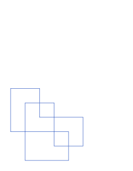
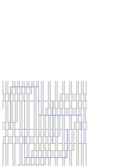
Figure 7. Constructing the diagram $\Pi$ in the proof of Lemma 5.1

Step 1. Put

$$\Pi_{1}=\{[\theta_{i,0};\theta_{i,3}]\times[\varphi_{i,3};\varphi_{i+1,0}],[\theta_{i,3};\theta_{i+1,0}]\times[\varphi_{i+1,0};\varphi_{i+1,3}]\}_{i=0,1,\ldots,n}.$$

Step 2. A rectangular diagram of a surface is uniquely defined by the union of its rectangles. Define $\Pi_{2}$ so that

$$\bigcup_{r\in\Pi_{2}}r=\overline{\bigcup_{r\in\Pi_{1}}r\,\setminus\bigcup_{r,r^{\prime}\in\Pi_{1};\,r\neq r^{\prime}}(r\cap r^{\prime})}.$$

Step 3. Define $\Pi_{3}$ by

$$\bigcup_{r\in\Pi_{3}}r=\overline{\bigcup_{r\in\Pi_{2}}r\,\triangle\bigcup_{i=1}^{n}\bigl{(}([\theta_{i,1};\theta_{i,2}]\cup[\theta_{i,4};\theta_{i,5}])\times\mathbb{S}^{1}\bigr{)}}.$$

Step 4. Finally, $\Pi$ is defined by

$$\bigcup_{r\in\Pi}r=\overline{\bigcup_{r\in\Pi_{3}}r\,\triangle\bigcup_{i=1}^{n}\bigl{(}\mathbb{S}^{1}\times([\varphi_{i,1};\varphi_{i,2}]\cup[\varphi_{i,4};\varphi_{i,5}])\bigr{)}}.$$

One can see that $R\subset\partial\Pi_{1}=\partial\Pi_{2}=\partial\Pi_{3}=\partial\Pi$. We claim that the combinatorial type of $\Pi$ is uniquely recovered from the dividing code of $\Pi$.

Indeed, suppose we have forgotten the values of $\theta_{i,j}$ and $\varphi_{i,j}$, and keep only the information about which pairs $(\theta_{i,j},\varphi_{i^{\prime},j^{\prime}})$ are vertices of which rectangles in $\Pi$ (this information is extracted from the dividing code).

For any $i\in\{1,2,\ldots,n\}$ and $j\in\{1,2,4,5\}$ the point $(\theta_{i,j},\varphi_{1,1})$ is a vertex of some rectangle in $\Pi$. Hence the cyclic order on $\{\theta_{i,j}\}_{i\in\{1,2,\ldots,n\};\,j\in\{1,2,4,5\}}\subset\mathbb{S}^{1}$ is prescribed by the dividing code.

For each $i\in\{1,2,\ldots,n\}$, we denote by $i^{-}$ the unique element of $\{1,2,\ldots,n\}$ such that $(\theta_{i^{-}};\theta_{i})\times\mathbb{S}^{1}$ does not contain vertices of $R$. One can see that for any $i\in\{1,2,\ldots,n\}$ there exist $j,j^{\prime}\in\{1,2,\ldots,n\}$ such that $(\theta_{i^{-},5},\varphi_{j,1})$, $(\theta_{i,0},\varphi_{j,1})$, $(\theta_{i,1},\varphi_{j,1})$, $(\theta_{i,2},\varphi_{j^{\prime},1})$, $(\theta_{i,3},\varphi_{j^{\prime},1})$, $(\theta_{i,4},\varphi_{j^{\prime},1})$ are vertices of some rectangles in $\Pi$. This prescribes the cyclic order on $\{\theta_{i^{-},5},\theta_{i,0},\theta_{i,1}\}$ and $\{\theta_{i,2},\theta_{i,3},\theta_{i,4}\}$ for any $i$. Therefore, the cyclic order on $\{\theta_{i,j}\}_{i\in\{1,2,\ldots,n\};\,j\in\{0,1,2,3,4,5\}}$ is completely determined by the dividing code.

Similarly, completely determined by the dividing code is the cyclic order on $\{\varphi_{i,j}\}_{i\in\{1,2,\ldots,n\};\,j\in\{0,1,2,3,4,5\}}$, and hence so is the combinatorial type of $\Pi$. ∎

Proof of Theorem 4.2.

By Lemma 5.1 we can find a rectangular diagram of a surface $\Pi$ such that $R_{1}\subset\partial\Pi$ and the combinatorial type of $\Pi$ is determined by the dividing code of $\Pi$. We pick such $\Pi$ and apply Proposition 5.1. Since the combinatorial type of $\Pi$ is determined by the dividing code of $\Pi$, we may strengthen the assertion of Proposition 5.1 in this case by claiming additionally that $\Pi^{\prime}=\Pi$ and $R_{2}^{\prime}=R_{1}$, which implies the assertion of the theorem. ∎

6. Triviality of the orientation-preserving symmetry groups of some knots

We use Rolfsen’s knot notation [39]. Knots with crossing number $\leqslant 10$ are well-studied (see [29, 30]), and the existing results about them imply the following.

Proposition 6.1.

The orientation-preserving symmetry group of each of the knots $9_{42}$, $9_{43}$, $9_{44}$, $9_{45}$, $10_{128}$, and $10_{160}$ is trivial.

The concrete sources for this statement are as follows. All the knots listed in Proposition 6.1 are known to be invertible (this can be seen from their pictures in [39]), so the assertion is equivalent to saying that the symmetry group of each of the knots is $\mathbb{Z}_{2}$.

The knots $9_{42}$, $9_{43}$, $9_{44}$, $9_{45}$ and $10_{128}$ are Montesinos knots (these are introduced in [33]):

$$9_{42}=K\Bigl{(}\frac{2}{5},\frac{1}{3},\frac{-1}{2}\Bigr{)},\ 9_{43}=K\Bigl{(}\frac{3}{5},\frac{1}{3},\frac{-1}{2}\Bigr{)},\ 9_{44}=K\Bigl{(}\frac{2}{5},\frac{2}{3},\frac{-1}{2}\Bigr{)},\ 9_{45}=K\Bigl{(}\frac{3}{5},\frac{2}{3},\frac{-1}{2}\Bigr{)},\ 10_{128}=K\Bigl{(}\frac{3}{7},\frac{1}{3},\frac{-1}{2}\Bigr{)}.$$

The knots $9_{42}$, $9_{43}$, $9_{44}$, $9_{45}$ are elliptic Montesinos knots, for which the symmetry group is computed by M. Sakuma [40]. The symmetry group of the knot $10_{128}$ is computed by M. Boileau and B. Zimmermann [1]. Both works are based on the technique which is due to F. Bonahon and L. Siebenmann [2].

The fact that the knot $10_{160}$ is not periodic is established by U. Lüdicke [31], and that it is not freely periodic is shown by R. Hartley [28].

Proposition 6.2.

The orientation-preserving symmetry group of the (topologically equivalent) knots $K_{1}$ and $K_{2}$ in Figure 4 is trivial.

Proof.

We use the classical methods of the above mentioned works with some technical improvements needed for reducing the amount of computations. ‘A direct check’ below refers to a computation that requires only a few minutes of a modern computer’s processor time and standard well known algorithms.

The first direct check is to see that the Alexander polynomial of $K_{1}$ and $K_{2}$ is

(1) $$\Delta(t)=t^{20}-t^{19}+t^{18}-3\,t^{17}+3\,t^{16}-5\,t^{15}+10\,t^{14}-5\,t^{13}+6\,t^{12}-14\,t^{11}+15\,t^{10}-\\ 14\,t^{9}+6\,t^{8}-5\,t^{7}+10\,t^{6}-5\,t^{5}+3\,t^{4}-3\,t^{3}+t^{2}-t+1.$$

According to Murasugi [34], if a knot has period $p$, with $p$ prime, then the Alexander polynomial of this knot reduced modulo $p$ is either the $p$th power of a polynomial with coefficients in $\mathbb{Z}_{p}$ or has a factor of the form $(1+t+\ldots+t^{d})^{p-1}$, where $d\geqslant 1$. It is a direct check that neither of these occurs in the case of the polynomial (1) for prime $p\leqslant 19$, and for $p>19$ the corresponding verification is trivial.

According to Hartley [28], to prove that our knot has not a free period equal to $p$ it suffices to ensure that $\Delta(t^{p})$ does not have a self-reciprocal factor of degree $\deg\Delta(t)=20$. For prime $p<100$ it can be checked directly that $\Delta(t^{p})$ is irreducible.

Suppose, for some prime $p>100$, we have a factorization $\Delta(t^{p})=f(t)\cdot g(t)$ with self-reciprocal $f(t),g(t)\in\mathbb{Z}[t]$ such that $\deg f=20$. Since $\Delta(0)=1$ we may assume $f(0)=1$ without loss of generality. For a self-reciprocal polynomial $q(t)$ of even degree we denote by $\widetilde{q}(t)$ the Laurent polynomial $t^{-(\deg q)/2}q(t)$.

For any $\alpha\in\{1,e^{\pi\mathbbm{i}/3},\mathbbm{i},e^{2\pi\mathbbm{i}/3},-1\}$ we have

1. $\alpha^{p}\in\{\alpha,\overline{\alpha}\}$;

2. $\widetilde{\Delta}(\alpha)=\widetilde{\Delta}(\overline{\alpha})$, $\widetilde{f}(\alpha)=\widetilde{f}(\overline{\alpha})$;

3. $\Delta(\alpha),f(\alpha),g(\alpha)\in\mathbb{Z}$.

For $a=(a_{1},a_{2},a_{3},a_{4},a_{5})$, denote by $\ell_{a}(t)\in\mathbb{R}[t]$ a self-reciprocal polynomial of even degree not exceeding $8$ such that $\widetilde{\ell}_{a}(t)$ takes the values $a_{1},a_{2},a_{3},a_{4},a_{5}$ at the points $t=1,e^{\pi\mathbbm{i}/3},\mathbbm{i},e^{2\pi\mathbbm{i}/3},-1$, respectively. This polynomial is clearly unique.

Now let $a\in\mathbb{Z}^{5}$ be the list of values of $\widetilde{f}$ at the points $1,e^{\pi\mathbbm{i}/3},\mathbbm{i},e^{2\pi\mathbbm{i}/3},-1$. Then the polynomial $t^{10}\bigl{(}\widetilde{f}(t)-\widetilde{\ell}(t)\bigr{)}$ is divisible by $(t^{6}-1)(t^{2}+1)$. Since this polynomial is also self-reciprocal, it is actually divisible by $(t^{6}-1)(t^{2}+1)(t-1)$. Thus, we have

(2) $$f(t)=t^{10}\,\widetilde{\ell}_{a}(t)+(t^{6}-1)(t^{2}+1)(t-1)\times{}\\ (t^{11}+b_{1}t^{10}+b_{2}t^{9}+b_{3}t^{8}+b_{4}t^{7}+b_{5}t^{6}+b_{5}t^{5}+b_{4}t^{4}+b_{3}t^{3}+b_{2}t^{2}+b_{1}t+1).$$

Since $\widetilde{\ell}_{a}$ may have non-zero coefficients only in front of $t^{k}$ with $k\in[-4;4]$, we see that $f(t)\in\mathbb{Z}[t]$ implies $b_{i}\in\mathbb{Z}$, $i=1,\ldots,5$, and $\ell_{a}(t)\in\mathbb{Z}[t]$.

One easily finds that the values of $\widetilde{\Delta}(t)$ at the points $t=1,e^{\pi\mathbbm{i}/3},\mathbbm{i},e^{2\pi\mathbbm{i}/3},-1$ are $1,-7,17,13,113$, respectively. Therefore, $a_{1},a_{2},a_{3},a_{4},a_{5}$ must be divisors of $1,-7,13,13,113$, respectively. Together with the condition $\ell_{a}(t)\in\mathbb{Z}[t]$ this leaves us only the following 32 options for $a$:

$$a =\pm(1,1,1,1,1), \ell_{a}(t) =\pm 1;$$

$$a =\pm(1,1,1,13,1), \ell_{a}(t) =\pm(-2t^{8}+2t^{7}-2t^{5}+5t^{4}-2t^{3}+2t-2);$$

$$a =\pm(1,1,17,1,1), \ell_{a}(t) =\pm(4t^{8}-4t^{6}+t^{4}-4t^{2}+4);$$

$$a =\pm(1,1,17,13,1), \ell_{a}(t) =\pm(2t^{8}+2t^{7}-4t^{6}-2t^{5}+5t^{4}-2t^{3}-4t^{2}+2t+2);$$

$$a =\pm(1,-1,1,1,113), \ell_{a}(t) =\pm(5t^{8}-9t^{7}+14t^{6}-19t^{5}+19t^{4}-19t^{3}+14t^{2}-9t+5);$$

$$a =\pm(1,-1,1,13,113), \ell_{a}(t) =\pm(3t^{8}-7t^{7}+14t^{6}-21t^{5}+23t^{4}-21t^{3}+14t^{2}-7t+3);$$

$$a =\pm(1,-1,17,1,113), \ell_{a}(t) =\pm(9t^{8}-9t^{7}+10t^{6}-19t^{5}+19t^{4}-19t^{3}+10t^{2}-9t+9);$$

$$a =\pm(1,-1,17,13,113), \ell_{a}(t) =\pm(7t^{8}-7t^{7}+10t^{6}-21t^{5}+23t^{4}-21t^{3}+10t^{2}-7t+7);$$

$$a =\pm(1,7,1,1,1), \ell_{a}(t) =\pm(-t^{8}-t^{7}+t^{5}+3t^{4}+t^{3}-t-1);$$

$$a =\pm(1,7,1,13,1), \ell_{a}(t) =\pm(-3t^{8}+t^{7}-t^{5}+7t^{4}-t^{3}+t-3);$$

$$a =\pm(1,7,17,1,1), \ell_{a}(t) =\pm(3t^{8}-t^{7}-4t^{6}+t^{5}+3t^{4}+t^{3}-4t^{2}-t+3);$$

$$a =\pm(1,7,17,13,1), \ell_{a}(t) =\pm(t^{8}+t^{7}-4t^{6}-t^{5}+7t^{4}-t^{3}-4t^{2}+t+1);$$

$$a =\pm(1,-7,1,1,113), \ell_{a}(t) =\pm(6t^{8}-8t^{7}+14t^{6}-20t^{5}+17t^{4}-20t^{3}+14t^{2}-8t+6);$$

$$a =\pm(1,-7,1,13,113), \ell_{a}(t) =\pm(4t^{8}-6t^{7}+14t^{6}-22t^{5}+21t^{4}-22t^{3}+14t^{2}-6t+4);$$

$$a =\pm(1,-7,17,1,113), \ell_{a}(t) =\pm(10t^{8}-8t^{7}+10t^{6}-20t^{5}+17t^{4}-20t^{3}+10t^{2}-8t+10);$$

$$a =\pm(1,-7,17,13,113), \ell_{a}(t) =\pm(8t^{8}-6t^{7}+10t^{6}-22t^{5}+21t^{4}-22t^{3}+10t^{2}-6t+8).$$

It is another direct check that all roots of $\Delta$ are located inside the circle $\{z\in\mathbb{C}:|z|<3/2\}$. Therefore, the roots of $f$ are contained in the circle $\{z\in\mathbb{C}:|z|<(3/2)^{1/p}\}$.

For $k\in\mathbb{N}$, denote by $p_{k}$ the $k$th Newton’s sum of $f$, that is, the sum of the $k$th powers of the roots. They must be integers, and we have the following estimate for their absolute values:

(3) $$|p_{k}|<20\cdot(3/2)^{k/p}.$$

Since $p>100$, this implies, in particular, that

(4) $$|p_{k}|\leqslant 20\quad\text{for }k=1,2,3,4,5.$$

Denote by $c_{k}$, $k=1,2,\ldots,19$, the coefficients of $f$: $f=1+c_{1}t+c_{2}t^{2}+\ldots+c_{19}t^{19}+t^{20}$, $c_{i}=c_{20-i}$. The first (equivalently: the last) five of them are related with $p_{i}$ by the following Newton’s identities:

$$-p_{1} =c_{1},$$

$$-p_{2} =c_{1}p_{1}+2c_{2},$$

$$-p_{3} =c_{1}p_{2}+c_{2}p_{1}+3c_{3},$$

$$-p_{4} =c_{1}p_{3}+c_{2}p_{2}+c_{3}p_{1}+4c_{4},$$

$$-p_{5} =c_{1}p_{4}+c_{2}p_{3}+c_{3}p_{2}+c_{4}p_{1}+5c_{5}.$$

This Diophantine system has exactly 971 865 solutions satisfying (4), which can be searched (another direct check). The coefficients $b_{1},b_{2},b_{3},b_{4},b_{5}$ in (2) can obviously be expressed through $c_{1},c_{2},c_{3},c_{4},c_{5}$. Thus, we get only $32\cdot 971865=31\,099\,680$ possible candidates for $f$, and it is the last direct check that the $k$th Newton’s sum of each of the obtained polynomials violates (3) for some $k\leqslant 31$ with any $p>100$. A contradiction.

We have thus established that the orientation preserving symmetry group of the knots $K_{1}$ and $K_{2}$ has no finite-order elements. It remains to ensure that these knots are not satellite knots (that is, they are hyperbolic). A way to verify this is explained in the Appendix. ∎

Proposition 6.2 is also directly confirmed by the SnapPy program [4]. For the reader’s convenience, we provide here a Dowker–Thistlethwaite code of the diagram of $K_{1}$ shown in Figure 4 (the numeration of the crossings starts from the arrowhead):

$-462$, $-346$, $-76$, $-218$, $156$, $472$, $356$, $66$, $208$, $126$, $-324$, $444$, $132$, $202$, $60$, $362$, $180$, $-478$, $-338$, $-284$, $-452$, $246$, $302$, $188$, $-460$, $400$, $-296$, $-492$, $-450$, $-286$, $-230$, $-88$, $-172$, $-122$, $-418$, $352$, $468$, $160$, $-276$, $220$, $154$, $474$, $334$, $384$, $412$, $502$, $-442$, $-24$, $134$, $200$, $58$, $40$, $146$, $-366$, $-184$, $-222$, $-80$, $8$, $314$, $264$, $380$, $416$, $506$, $-168$, $-92$, $-234$, $-290$, $-446$, $196$, $54$, $456$, $-488$, $-46$, $-282$, $-340$, $-480$, $-430$, $-272$, $-116$, $-424$, $-372$, $-256$, $508$, $20$, $504$, $414$, $382$, $266$, $-84$, $-226$, $36$, $150$, $278$, $344$, $-396$, $-458$, $-52$, $-294$, $-494$, $-448$, $-288$, $-232$, $-90$, $-170$, $-124$, $68$, $354$, $470$, $158$, $-274$, $-428$, $152$, $476$, $336$, $386$, $410$, $500$, $94$, $-22$, $136$, $198$, $56$, $42$, $-392$, $-140$, $192$, $50$, $2$, $320$, $-350$, $-72$, $-214$, $-12$, $-332$, $176$, $312$, $114$, $426$, $-482$, $-342$, $106$, $304$, $388$, $408$, $498$, $-96$, $-238$, $402$, $250$, $-142$, $-394$, $-104$, $-364$, $-182$, $-224$, $-82$, $-10$, $-216$, $-74$, $-348$, $-464$, $166$, $128$, $206$, $64$, $358$, $-268$, $-434$, $-32$, $306$, $108$, $368$, $-484$, $162$, $466$, $-376$, $-420$, $-120$, $-174$, $-86$, $-228$, $38$, $148$, $280$, $-186$, $4$, $318$, $260$, $-70$, $-212$, $-14$, $-330$, $-436$, $-30$, $-102$, $-244$, $454$, $144$, $486$, $-252$, $194$, $-138$, $-242$, $-100$, $-28$, $-438$, $-328$, $-16$, $-210$, $378$, $262$, $316$, $6$, $-78$, $112$, $310$, $178$, $360$, $62$, $204$, $130$, $-236$, $292$, $496$, $406$, $390$, $-44$, $-490$, $-298$, $398$, $254$, $164$, $-258$, $-374$, $-422$, $-118$, $-270$, $-432$, $-34$, $308$, $110$, $370$, $-48$, $190$, $300$, $248$, $404$, $-240$, $-98$, $-26$, $-440$, $-326$, $-18$, $-322$.

7. Applications

Theorem 7.1.

There exists an algorithm that decides in finite time whether or not two given Legendrian knots, $L_{1}$ and $L_{2}$, say, are equivalent provided that they are topologically equivalent and have trivial orientation-preserving symmetry group.

Proof.

It is understood that $L_{1}$ and $L_{2}$ are presented in a combinatorial way that allows to recover actual curves in $\mathbb{R}^{3}$. Whichever presentation is chosen, it can always be converted into rectangular diagrams. So, we assume that we are given two rectangular diagrams of a knot, $R_{1}$ and $R_{2}$, say, such that $\mathscr{L}_{+}(R_{1})\ni L_{1}$ and $\mathscr{L}_{+}(R_{2})\ni L_{2}$.

By [8, Theorem 7] there exists a rectangular diagram of a knot $R_{3}$ such that $\mathscr{L}_{+}(R_{3})=\mathscr{L}_{+}(R_{1})$ and $\mathscr{L}_{-}(R_{3})=\mathscr{L}_{-}(R_{2})$. According to Theorem 4.1 this is equivalent to saying that there exists a sequence of elementary moves transforming $R_{1}$ to $R_{3}$ (respectively, $R_{3}$ to $R_{2}$) including only exchange moves and type I (respectively, type II) stabilizations and destabilizations. Therefore, such an $R_{3}$ can be found by an exhaustive search of sequences of elementary moves starting at $R_{1}$ in which all type I stabilizations and destabilizations occur before all type II ones. Indeed, the combinatorial types of such sequences are enumerable.The search terminates once a sequence with the above properties arriving at $R_{2}$ is encountered. By [8, Theorem 7] this must eventually happen.

Once $R_{3}$ is found we check whether or not it is related to $R_{2}$ by a sequence of exchange moves. The latter can produce only finitely many combinatorial types of diagrams from the given one, so this process is finite. According to Theorem 4.2 the diagrams $R_{2}$ and $R_{3}$ are related by a sequence of exchange moves if and only if $\mathscr{L}_{+}(R_{2})=\mathscr{L}_{+}(R_{3})$, which is equivalent to $\mathscr{L}_{+}(R_{1})=\mathscr{L}_{+}(R_{2})$. ∎

Now we use Theorem 4.2 to establish some facts that are left in [5] as conjectures. These involve knots with trivial orientation-preserving symmetry group that are listed in Proposition 6.1 above.

For a rectangular diagram of a knot $R$, the set of all rectangular diagrams obtained from $R$ by a sequence of exchange moves is called the exchange class of $R$.

In what follows we use the following notation system. $\xi_{+}$-Legendrian classes of knots having topological type $m_{n}$ are denoted $m_{n}^{k+}$, $k=1,2,\ldots$, or simply $m_{n}^{+}$ if we need to consider only one Legendrian class and its images under $\mu$ and orientation reversal. Similarly, for $\xi_{-}$-Legendrian we use notation of the form $m_{n}^{k-}$ or $m_{n}^{-}$, and for exchange classes $m_{n}^{k\mathrm{R}}$ or $m_{n}^{\mathrm{R}}$.

The $\xi_{\pm}$-Legendrian classes and exchange classes of our interest are defined by specifying a representative. In order to help the reader to see the correspondence with the notation of [5] we define the $\xi_{-}$-Legendrian classes via their mirror images, which are $\xi_{+}$-Legendrian classes.

We use the same notation for natural operations on (exchange classes of) rectangular diagrams as for Legendrian knots: ‘$-$’ for orientation reversal, $r_{\medvert}$ and $r_{-}$ for the horizontal and the vertical flip, respectively, and $\mu$ for $r_{\medvert}\circ r_{-}$. One can see that if $X$ is an exchange class, then $\mathscr{L}_{\pm}(-X)=-\mathscr{L}_{\pm}(X)$, $\mathscr{L}_{\pm}(\mu(X))=\mu(\mathscr{L}_{\pm}(X))$, $\mathscr{L}_{\pm}(r_{\medvert}(X))=r_{\medvert}(\mathscr{L}_{\mp}(X))$.

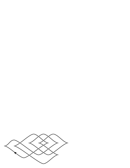
Figure 8. Legendrian knots in Proposition 7.1 and an exchange class representing both

Proposition 7.1.

For the classes $9_{42}^{+}$ and $9_{42}^{-}$ whose representatives are shown in Figure 8, we have $9_{42}^{+}{}=-9_{42}^{+}\neq\mu(9_{42}^{+})$ and $9_{42}^{-}\neq-9_{42}^{-}{}=\mu(9_{42}^{-})$.

Proof.

We use the exchange class $9_{42}^{\mathrm{R}}$ of the diagram shown in Figure 8 on the right. Black vertices are positive, and white ones are negative.

It is an easy check that the diagram representing the class $9_{42}^{\mathrm{R}}$ in Figure 8 admits no non-trivial (that is, changing the combinatorial type) exchange move, and its combinatorial type changes under reversing the orientation and under its composition with the rotation $\mu$. We conclude from this that

(5) $$9_{42}^{\mathrm{R}}\neq-9_{42}^{\mathrm{R}}\quad\text{and}\quad-9_{42}^{\mathrm{R}}\neq\mu(9_{42}^{\mathrm{R}}).$$

Now we verify directly that $S_{\overrightarrow{\mathrm{I}}}(9_{42}^{\mathrm{R}})=S_{\overrightarrow{\mathrm{I}}}(-9_{42}^{\mathrm{R}})$:

$$\begin{array}[]{ccccccccccccccccc}\includegraphics[width=30.0pt]{aux1216.eps}&\kern-6.00006pt\raisebox{12.0pt}{$\rightarrow$}\kern-6.00006pt&\includegraphics[width=30.0pt]{aux1215.eps}&\kern-6.00006pt\raisebox{12.0pt}{$\rightarrow$}\kern-6.00006pt&\includegraphics[width=30.0pt]{aux1214.eps}&\kern-6.00006pt\raisebox{12.0pt}{$\rightarrow$}\kern-6.00006pt&\includegraphics[width=30.0pt]{aux1213.eps}&\kern-6.00006pt\raisebox{12.0pt}{$\rightarrow$}\kern-6.00006pt&\includegraphics[width=30.0pt]{aux1212.eps}&\kern-6.00006pt\raisebox{12.0pt}{$\rightarrow$}\kern-6.00006pt&\includegraphics[width=30.0pt]{aux1211.eps}&\kern-6.00006pt\raisebox{12.0pt}{$\rightarrow$}\kern-6.00006pt&\includegraphics[width=30.0pt]{aux1210.eps}&\kern-6.00006pt\raisebox{12.0pt}{$\rightarrow$}\kern-6.00006pt&\includegraphics[width=30.0pt]{aux1209.eps}&\kern-6.00006pt\raisebox{12.0pt}{$\rightarrow$}\kern-6.00006pt&\includegraphics[width=30.0pt]{aux1208.eps}\\ &&&&&&&&&&&&&&&&\downarrow\\ &&\includegraphics[width=30.0pt]{aux1200.eps}&\kern-6.00006pt\raisebox{12.0pt}{$\leftarrow$}\kern-6.00006pt&\includegraphics[width=30.0pt]{aux1201.eps}&\kern-6.00006pt\raisebox{12.0pt}{$\leftarrow$}\kern-6.00006pt&\includegraphics[width=30.0pt]{aux1202.eps}&\kern-6.00006pt\raisebox{12.0pt}{$\leftarrow$}\kern-6.00006pt&\includegraphics[width=30.0pt]{aux1203.eps}&\kern-6.00006pt\raisebox{12.0pt}{$\leftarrow$}\kern-6.00006pt&\includegraphics[width=30.0pt]{aux1204.eps}&\kern-6.00006pt\raisebox{12.0pt}{$\leftarrow$}\kern-6.00006pt&\includegraphics[width=30.0pt]{aux1205.eps}&\kern-6.00006pt\raisebox{12.0pt}{$\leftarrow$}\kern-6.00006pt&\includegraphics[width=30.0pt]{aux1206.eps}&\kern-6.00006pt\raisebox{12.0pt}{$\leftarrow$}\kern-6.00006pt&\includegraphics[width=30.0pt]{aux1207.eps}\end{array},$$

and $S_{\overrightarrow{\mathrm{II}}}(-9_{42}^{\mathrm{R}})=S_{\overrightarrow{\mathrm{II}}}(\mu(9_{42}^{\mathrm{R}}))$:

$$\begin{array}[]{ccccccccc}\includegraphics[width=30.0pt]{aux1309.eps}&\kern-6.00006pt\raisebox{12.0pt}{$\rightarrow$}\kern-6.00006pt&\includegraphics[width=30.0pt]{aux1308.eps}&\kern-6.00006pt\raisebox{12.0pt}{$\rightarrow$}\kern-6.00006pt&\includegraphics[width=30.0pt]{aux1307.eps}&\kern-6.00006pt\raisebox{12.0pt}{$\rightarrow$}\kern-6.00006pt&\includegraphics[width=30.0pt]{aux1306.eps}&\kern-6.00006pt\raisebox{12.0pt}{$\rightarrow$}\kern-6.00006pt&\includegraphics[width=30.0pt]{aux1305.eps}\\ &&&&&&&&\downarrow\\ \includegraphics[width=30.0pt]{aux1300.eps}&\kern-6.00006pt\raisebox{12.0pt}{$\leftarrow$}\kern-6.00006pt&\includegraphics[width=30.0pt]{aux1301.eps}&\kern-6.00006pt\raisebox{12.0pt}{$\leftarrow$}\kern-6.00006pt&\includegraphics[width=30.0pt]{aux1302.eps}&\kern-6.00006pt\raisebox{12.0pt}{$\leftarrow$}\kern-6.00006pt&\includegraphics[width=30.0pt]{aux1303.eps}&\kern-6.00006pt\raisebox{12.0pt}{$\leftarrow$}\kern-6.00006pt&\includegraphics[width=30.0pt]{aux1304.eps}\end{array}.$$

By Theorem 4.1 this implies

(6) $$\mathscr{L}_{+}(9_{42}^{\mathrm{R}})=\mathscr{L}_{+}(-9_{42}^{\mathrm{R}})\quad\text{and}\quad\mathscr{L}_{-}(-9_{42}^{\mathrm{R}})=\mathscr{L}_{-}(\mu(9_{42}^{\mathrm{R}})).$$

From Proposition 6.1 and Theoremd 4.2 we conclude:

$$\eqref{9-42-ne-eq}\ \&\ \eqref{9-42-eq}\quad\Rightarrow\quad\mathscr{L}_{-}(9_{42}^{\mathrm{R}})\neq\mathscr{L}_{-}(-9_{42}^{\mathrm{R}})\quad\text{and}\quad\mathscr{L}_{+}(-9_{42}^{\mathrm{R}})\neq\mathscr{L}_{+}(\mu(9_{42}^{\mathrm{R}})).$$

The front projections in Figure 8 are obtained as described in Section 4 (see Figure 6) from rectangular diagrams that can be easily guessed from the pictures. Using Theorem 4.1 we find that $9_{42}^{+}=\mathscr{L}_{+}(9_{42}^{\mathrm{R}})$:

$$\begin{array}[]{ccccccccccccccc}\includegraphics[width=30.0pt]{aux1000.eps}&\kern-6.00006pt\raisebox{12.0pt}{$\rightarrow$}\kern-6.00006pt&\includegraphics[width=30.0pt]{aux1001.eps}&\kern-6.00006pt\raisebox{12.0pt}{$\rightarrow$}\kern-6.00006pt&\includegraphics[width=30.0pt]{aux1002.eps}&\kern-6.00006pt\raisebox{12.0pt}{$\rightarrow$}\kern-6.00006pt&\includegraphics[width=30.0pt]{aux1003.eps}&\kern-6.00006pt\raisebox{12.0pt}{$\rightarrow$}\kern-6.00006pt&\includegraphics[width=30.0pt]{aux1004.eps}&\kern-6.00006pt\raisebox{12.0pt}{$\rightarrow$}\kern-6.00006pt&\includegraphics[width=30.0pt]{aux1005.eps}&\kern-6.00006pt\raisebox{12.0pt}{$\rightarrow$}\kern-6.00006pt&\includegraphics[width=30.0pt]{aux1006.eps}&\kern-6.00006pt\raisebox{12.0pt}{$\rightarrow$}\kern-6.00006pt&\includegraphics[width=30.0pt]{aux1007.eps}\\ &&&&&&&&&&&&&&\downarrow\\ \includegraphics[width=30.0pt]{aux1015.eps}&\kern-6.00006pt\raisebox{12.0pt}{$\leftarrow$}\kern-6.00006pt&\includegraphics[width=30.0pt]{aux1014.eps}&\kern-6.00006pt\raisebox{12.0pt}{$\leftarrow$}\kern-6.00006pt&\includegraphics[width=30.0pt]{aux1013.eps}&\kern-6.00006pt\raisebox{12.0pt}{$\leftarrow$}\kern-6.00006pt&\includegraphics[width=30.0pt]{aux1012.eps}&\kern-6.00006pt\raisebox{12.0pt}{$\leftarrow$}\kern-6.00006pt&\includegraphics[width=30.0pt]{aux1011.eps}&\kern-6.00006pt\raisebox{12.0pt}{$\leftarrow$}\kern-6.00006pt&\includegraphics[width=30.0pt]{aux1010.eps}&\kern-6.00006pt\raisebox{12.0pt}{$\leftarrow$}\kern-6.00006pt&\includegraphics[width=30.0pt]{aux1009.eps}&\kern-6.00006pt\raisebox{12.0pt}{$\leftarrow$}\kern-6.00006pt&\includegraphics[width=30.0pt]{aux1008.eps}\end{array},$$

and $9_{42}^{-}=\mathscr{L}_{-}(9_{42}^{\mathrm{R}})$:

$$\begin{array}[]{ccccccccccccccccc}\includegraphics[width=30.0pt]{aux1100.eps}&\kern-6.00006pt\raisebox{12.0pt}{$\rightarrow$}\kern-6.00006pt&\includegraphics[width=30.0pt]{aux1101.eps}&\kern-6.00006pt\raisebox{12.0pt}{$\rightarrow$}\kern-6.00006pt&\includegraphics[width=30.0pt]{aux1102.eps}&\kern-6.00006pt\raisebox{12.0pt}{$\rightarrow$}\kern-6.00006pt&\includegraphics[width=30.0pt]{aux1103.eps}&\kern-6.00006pt\raisebox{12.0pt}{$\rightarrow$}\kern-6.00006pt&\includegraphics[width=30.0pt]{aux1104.eps}&\kern-6.00006pt\raisebox{12.0pt}{$\rightarrow$}\kern-6.00006pt&\includegraphics[width=30.0pt]{aux1105.eps}&\kern-6.00006pt\raisebox{12.0pt}{$\rightarrow$}\kern-6.00006pt&\includegraphics[width=30.0pt]{aux1106.eps}&\kern-6.00006pt\raisebox{12.0pt}{$\rightarrow$}\kern-6.00006pt&\includegraphics[width=30.0pt]{aux1107.eps}&\kern-6.00006pt\raisebox{12.0pt}{$\rightarrow$}\kern-6.00006pt&\includegraphics[width=30.0pt]{aux1108.eps}\\ \end{array},$$

which completes the proof. ∎

The proof of Proposition 7.1 is summarized in Figure 9. In what follows we present the proofs by similar schemes omitting the verbal description. For a routine check of all equalities and inequalities of exchange classes used in the proofs the reader is referred to [12].

In the proofs of Propositions 7.3, 7.4, and 7.6 we may also silently use symmetries: an inequality $X\neq Y$, where $X$ and $Y$ are some Legendrian or exchange classes, is equivalent to any of $-X\neq-Y$, $\mu(X)\neq\mu(Y)$. Another use of symmetries is as follows. If $X$ and $Y$ are Legendrian classes such that $X=-X$ and $Y\neq-Y$ (similarly for $\mu$ or $-\mu$ in place of ‘$-$’), then we immediately know that $X\notin\{Y,-Y,\mu(Y),-\mu(Y)\}$.

Figure 9. Proof of Proposition 7.1

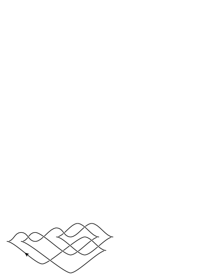
Figure 10. Legendrian knots in Proposition 7.2

Proposition 7.2.

For the $\xi_{\pm}$-Legendrian classes whose representatives are shown in Figure 10, we have $9_{43}^{+}\neq-9_{43}^{+}$ and $9_{43}^{-}\neq-\mu(9_{43}^{-})$.

The proof is presented in Figure 11.

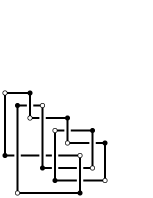
Figure 11. Proof of Proposition 7.2

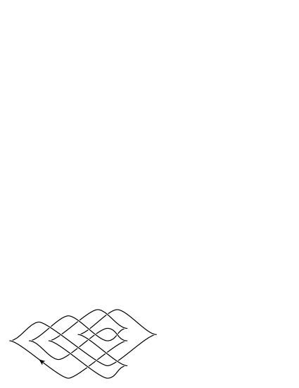
Figure 12. The knots in Proposition 7.3

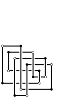
Figure 13. Exchange classes used in the proof of Proposition 7.3

Proposition 7.3.

For the $\xi_{\pm}$-Legendrian classes whose representatives are shown in Figure 12 the following holds:

1. the $\xi_{+}$-Legendrian classes $9_{44}^{1+}$, $9_{44}^{2+}$, $9_{44}^{3+}$, $-\mu(9_{44}^{1+})$, $-\mu(9_{44}^{2+})$, $-\mu(9_{44}^{3+})$ are pairwise distinct;

2. for $k\in\{1,2,3,4\}$ the $\xi_{+}$-Legendrian classes $S_{+}^{k}(9_{44}^{1+})$, $S_{+}^{k}(9_{44}^{2+})$, and $S_{+}^{k}(9_{44}^{3+})$ are pairwise distinct;

3. the $\xi_{-}$-Legendrian classes $9_{44}^{-}$ and $-9_{44}^{-}$ are distinct.

Proof.

Representatives of the exchange classes involved in the proof are shown in Figure 13. The fact that $9_{44}^{1+},-\mu(9_{44}^{1+})\notin\{9_{44}^{2+},9_{44}^{3+}\}$ and $S_{+}^{k}(9_{44}^{1+})\notin\bigl{\{}S_{+}^{k}(9_{44}^{2+}),S_{+}^{k}(9_{44}^{3+})\bigr{\}}$ for any $k\in\mathbb{N}$, is established in [5]. The proof of the remaining claims is presented in Figure 14 (where some of the known facts are also reproved).

Figure 14. Proof of Proposition 7.3

∎

Remark 7.1.

It is conjectured in [5] that the $\xi_{+}$-Legendrian classes $S_{+}^{k}(9_{44}^{2+})$ and $S_{+}^{k}(9_{44}^{3+})$ are distinct for any $k\in\mathbb{N}$, not only $k\leqslant 4$. The method of this paper allows, in principle, to test the claim for any fixed $k$, and this has been done by the authors for $k\leqslant 4$. (For larger $k$, the simple—and far from being optimized—exhaustive search, which we used to test diagrams for exchange-equivalence, takes too much time.)

Proving the claim for all $k$ is equivalent to distinguishing certain transverse knots. The present technique has been upgraded in [7] to an algorithmic solution of this problem (in the case of knots with trivial orientation-preserving symmetry group). This reduces the task of verifying the inequality $S_{+}^{k}(9_{44}^{2+})\neq S_{+}^{k}(9_{44}^{3+})$ for all $k\in\mathbb{N}$ to a finite exhaustive search, which is still to be done.

A similar remark applies to part (iii) of Proposition 7.4 and parts (ii) of Propositions 7.5 and 7.6. In the last two cases the required exhaustive search appears to be trivial, so the question for the knots $10_{128}$ and $10_{160}$ is settled in [7] completely.

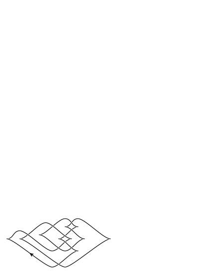
Figure 15. The knots in Proposition 7.4

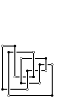
Figure 16. Exchange classes used in the proof of Proposition 7.4

Proposition 7.4.

For the $\xi_{\pm}$-Legendrian classes whose representatives are shown in Figure 15 the following holds:

1. $9_{45}^{1+}$, $9_{45}^{2+}$, $9_{45}^{3+}$, $-\mu(9_{45}^{1+})$, and $-\mu(9_{45}^{3+})$ are pairwise distinct;

2. $9_{45}^{1-}$, $-9_{45}^{1-}$, $\mu(9_{45}^{1-})$, $-\mu(9_{45}^{1-})$, $9_{45}^{2-}$, and $\mu(9_{45}^{2-})$ are pairwise distinct;

3. for $k\in\{1,2,3\}$ the $\xi_{-}$-Legendrian classes $S_{+}^{k}(9_{45}^{2-})$ and $S_{+}^{k}\bigl{(}-\mu(9_{45}^{2-})\bigr{)}$ are distinct.

Proof.

Representatives of the exchange classes involved in the proof are shown in Figure 16. It is established in [5] that $9_{45}^{2+}=-\mu(9_{45}^{2+})$. So, to prove part (i) of the proposition it suffices to show that $9_{45}^{1+}$, $9_{45}^{3+}$, $-\mu(9_{45}^{1+})$, and $-\mu(9_{45}^{3+})$ are pairwise distinct. The proof of this and of part (iii) is presented in Figure 17.

Figure 17. Proof of parts (i) and (iii) of Proposition 7.4

Figure 18. Proof of part (ii) of Proposition 7.4

It is already established in [5] that $9_{45}^{2-}=-9_{45}^{2-}\notin\bigl{\{}9_{45}^{1-},-9_{45}^{1-},\mu(9_{45}^{1-}),-\mu(9_{45}^{1-}),\mu(9_{45}^{2-})\bigr{\}}$, so it remains to show that $9_{45}^{1-}$, $-9_{45}^{1-}$, $\mu(9_{45}^{1-})$, and $-\mu(9_{45}^{1-})$ are pairwise distinct. To this end, it suffices to show that some three of these four classes are pairwise distinct. This is done in Figure 18. ∎

Proposition 7.5.

For the Legendrian classes whose representatives are shown in Figure 19 the following holds:

1. the Legendrian classes $10_{128}^{1+}$, $10_{128}^{2+}$, $-\mu\bigl{(}10_{128}^{1+}\bigr{)}$, and $-\mu\bigl{(}10_{128}^{2+}\bigr{)}$ are pairwise distinct;

2. for any $k\in\{1,2,3,4\}$ the Legendrian classes $S_{-}^{k}(10_{128}^{1+})=S_{-}^{k}(10_{128}^{2+})$ and $S_{-}^{k}\bigl{(}-\mu(10_{128}^{1+})\bigr{)}=S_{-}^{k}\bigl{(}-\mu(10_{128}^{2+})\bigr{)}$ are distinct.

Proof.

The proof is presented in Figure 20.

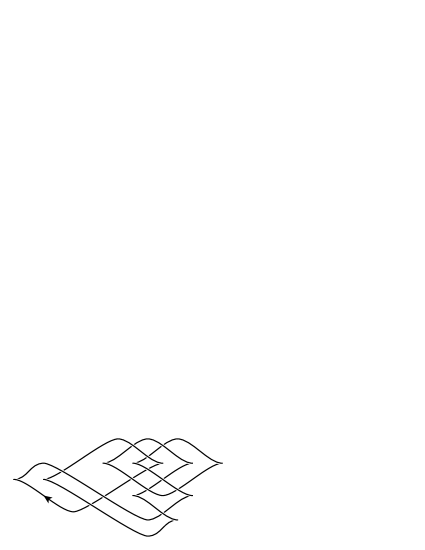
Figure 19. Knots in Proposition 7.5

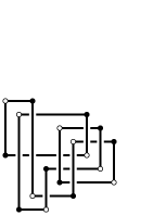
Figure 20. Proof of Proposition 7.5

∎

Proposition 7.6.

For the Legendrian classes whose representatives are shown in Figure 21 the following holds:

1. the classes $10_{160}^{1+}{}=-10_{160}^{1+}$, $\mu\bigl{(}10_{160}^{1+}\bigr{)}$, $10_{160}^{2+}$, $-10_{160}^{2+}$, $\mu\bigl{(}10_{160}^{2+}\bigr{)}$, and $-\mu\bigl{(}10_{160}^{2+}\bigr{)}$ are pairwise distinct;

2. for any $k\in\{1,2,3,4\}$ the classes $S_{-}^{k}(10_{160}^{2+})$ and $S_{-}^{k}(-10_{160}^{2+})$ are distinct.

Proof.

The proof is presented in Figure 22. (The $\xi_{-}$-Legendrian class $10_{160}^{-}$ can be guessed from the scheme. We don’t provide a picture as this class is not involved in any of our statements.)

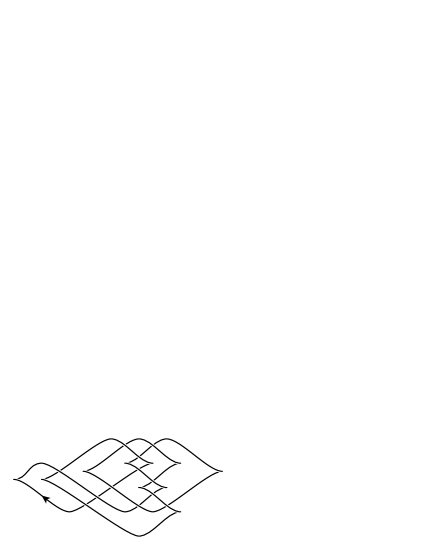
Figure 21. Knots in Proposition 7.6

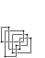
Figure 22. Proof of Proposition 7.6

∎

Remark 7.2.

The fact that $10_{160}^{1+}\notin\bigl{\{}10_{160}^{2+},-10_{160}^{2+},\mu(10_{160}^{2+}),-\mu(10_{160}^{2+})\bigr{\}}$ and $10_{160}^{1+}=-10_{160}^{1+}$ is established already in [5].

Proof of Theorem 2.1.

The front projections of $K_{1}$ and $K_{2}$ shown in Figure 4 are produced from two rectangular diagrams $R_{1}$ and $R_{2}$, respectively, via the procedure described in Section 4 and illustrated in Figure 6. Thus, we have $K_{i}\in\mathscr{L}_{+}(R_{i})$, $i=1,2$.

Now we recall the origin of $R_{1}$, $R_{2}$. Shown in Figure 35 of [9] is a rectangular diagram $\Pi$ of a surface such that:

1. the associated surface $\widehat{\Pi}$ is an annulus;

2. the relative Thurston–Bennequin numbers $\mathop{tb}\nolimits(\widehat{R}_{i};\widehat{\Pi})$, $i=1,2$, vanish;

3. $\widehat{\Pi}$ can be endowed with an orientation so that $\partial\widehat{\Pi}=\widehat{R}_{1}\cup(-\widehat{R}_{2})$;

4. $\Pi$ has the form $\{r_{i}\}_{i=1,2,\ldots,74}$, where, for each $i=1,\ldots,74$ the intersection $r_{i-1}\cap r_{i}$ is the bottom left vertex of $r_{i}$ (we put $r_{0}=r_{74}$).

The last condition in this list means that there are $\theta_{0},\theta_{1},\ldots,\theta_{74}=\theta_{0}\in\mathbb{S}^{1}$ and $\varphi_{0},\varphi_{1},\ldots,\varphi_{74}=\varphi_{0}\in\mathbb{S}^{1}$ such that $r_{i}=[\theta_{i-1};\theta_{i}]\times[\varphi_{i-1};\varphi_{i}]$ and $R_{1}\cup R_{2}=\{(\theta_{i-1},\varphi_{i}),(\theta_{i},\varphi_{i-1})\}_{i=1,\ldots,74}$. Moreover, the signs of the vertices $(\theta_{i-1},\varphi_{i})$ and $(\theta_{i},\varphi_{i-1})$ in $R_{1}\cup R_{2}$ are opposite.

We now show that a sequence of elementary moves including a type II stabilization, exchange moves, and a type II destabilization transforms $R_{1}\cup R_{2}$ to a rectangular diagram of a link in which the connected components become combinatorially equivalent. To this end, pick an $\varepsilon>0$ smaller than one half of the length of any interval $[\theta_{i};\theta_{j}]$ and $[\varphi_{i};\varphi_{j}]$, $i\neq j$, and make the following replacements in $R_{1}\cup R_{2}$:

$$(\theta_{1},\varphi_{0}) \rightsquigarrow(\theta_{0}-\varepsilon,\varphi_{0}),(\theta_{0}-\varepsilon,\varphi_{1}-\varepsilon),(\theta_{1},\varphi_{1}-\varepsilon) \text{(type~{}II stabilization)},$$

$$(\theta_{1},\varphi_{1}-\varepsilon),(\theta_{1},\varphi_{2}) \rightsquigarrow(\theta_{2}-\varepsilon,\varphi_{1}-\varepsilon),(\theta_{2}-\varepsilon,\varphi_{2}) \text{(exchange)},$$

$$(\theta_{2}-\varepsilon,\varphi_{2}),(\theta_{3},\varphi_{2}) \rightsquigarrow(\theta_{2}-\varepsilon,\varphi_{3}-\varepsilon),(\theta_{3},\varphi_{3}-\varepsilon) \text{(exchange)},$$

$$(\theta_{3},\varphi_{3}-\varepsilon),(\theta_{3},\varphi_{4}) \rightsquigarrow(\theta_{4}-\varepsilon,\varphi_{3}-\varepsilon),(\theta_{4}-\varepsilon,\varphi_{4}) \text{(exchange)},$$

$$\ldots$$

$$(\theta_{72}-\varepsilon,\varphi_{72}),(\theta_{73},\varphi_{72}) \rightsquigarrow(\theta_{72}-\varepsilon,\varphi_{73}-\varepsilon),(\theta_{73},\varphi_{73}-\varepsilon) \text{(exchange)},$$

$$(\theta_{73},\varphi_{73}-\varepsilon),(\theta_{73},\varphi_{0}),(\theta_{0}+\varepsilon,\varphi_{0}) \rightsquigarrow(\theta_{0}-\varepsilon,\varphi_{73}-\varepsilon) \text{(type~{}II destabilization)}.$$

This sequence of moves is illustrated in Figure 23.

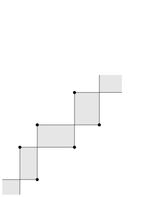
Figure 23. Transforming one of $R_{1}$ and $R_{2}$ to the other by elementary moves

This proves that $\mathscr{L}_{-}(R_{1})=\mathscr{L}_{-}(R_{2})$. The diagrams $R_{1}$ and $R_{2}$ are not combinatorially equivalent and do not admit any non-trivial exchange move. The knots represented by $R_{1}$ and $R_{2}$ have trivial orientation-preserving symmetry group by Proposition 6.2. Therefore, by Theorem 4.2, $\mathscr{L}_{+}(R_{1})\neq\mathscr{L}_{+}(R_{2})$. ∎

8. Appendix: $K_{1}$ and $K_{2}$ are not satellite knots

Here we explain how to verify, with very little computations, that the complement of $K_{1}$ (and $K_{2}$) contains no incompressible non-boundary-parallel torus. To do so we use a method that can be viewed as a modification of Haken’s method of normal surfaces, which allows one, in general, to find all incompressible surfaces of minimal genus. Haken’s algorithm in general has very high computational complexity, which makes it infeasible to implement in most cases. However, in certain cases including our particular one, a modified version of Haken’s method can be efficiently used to search all incompressible surfaces of non-negative Euler characteristic.

First we describe the general idea for the reader well familiar with the difficulties in using Haken’s method in practice. Haken’s normal surfaces are encoded by certain normal coordinates $x_{1},\ldots,x_{N}$, which take integer values. To determine a normal surface they must satisfy a bunch of conditions that are naturally partitioned into the following three groups:

1. non-negativity conditions, which are the inequalities $x_{i}\geqslant 0$, $i=1,\ldots,N$;

2. matching conditions, which are linear equations with integer coefficients;

3. compatibility conditions, which are equations of the form $x_{i}x_{j}=0$ for some set of pairs $(i,j)$.

The Euler characteristic of a normal surface $F$ can be expressed as a linear combination of the normal coordinates of $F$ in numerous ways, and some of these expressions have only non-positive coefficients. If we are looking for normal surfaces of non-negative Euler characteristic, for any such expression $\sum_{i}a_{i}x_{i}$ with non-positive $a_{i}$’s, we may add the inequality $\sum_{i}a_{i}x_{i}\geqslant 0$ to the system. Together with the non-negativity conditions this implies $x_{i}=0$ whenever $a_{i}<0$. This reduces the number of variables in the system, and chances are that, after the reduction, the space of solutions of the system of matching equations alone has very small dimension.

Now we turn to our concrete case. The idea explained above will be realized in quite different terms. The reduction of variables will occur in Lemma 8.2.

The rectangular diagrams from which the Legendrian knots $K_{1}$ and $K_{2}$ shown in Figure 4 are produced have $37$ edges of each direction. For this reason we rescale the coordinates $\theta,\varphi$ on $\mathbb{T}^{2}$ so that they take values in $\mathbb{R}/(37\cdot\mathbb{Z})$, and the vertices of the diagrams will form a subset of $\mathbb{Z}_{37}\times\mathbb{Z}_{37}$.

We will work with the knot $K_{1}$. The corresponding rectangular diagram of a knot, which we denote by $R$, has the following list of vertices:

$$(0,13),(0,28),(1,14),(1,35),(2,15),(2,36),(3,0),(3,19),(4,1),(4,22),(5,6),(5,23),(6,7),(6,24),\\ (7,9),(7,25),(8,10),(8,26),(9,11),(9,27),(10,12),(10,29),(11,13),(11,34),(12,20),(12,35),\\ (13,21),(13,36),(14,8),(14,22),(15,9),(15,31),(16,10),(16,32),(17,11),(17,33),(18,18),(18,34),\\ (19,4),(19,19),(20,5),(20,20),(21,6),(21,21),(22,7),(22,23),(23,8),(23,30),(24,12),(24,31),\\ (25,16),(25,32),(26,17),(26,33),(27,2),(27,18),(28,3),(28,24),(29,4),(29,28),(30,14),(30,29),\\ (31,15),(31,30),(32,0),(32,16),(33,1),(33,17),(34,2),(34,25),(35,3),(35,26),(36,5),(36,27).$$

According to [9, Theorem 1] any incompressible torus in the complement of $\widehat{R}$ is isotopic to a surface of the form $\widehat{\Pi}$, where $\Pi$ is a rectangular diagram of a surface. Let such a diagram $\Pi$ be chosen so that the number of rectangles in $\Pi$ is as minimal as possible (which is equivalent to requesting that $\widehat{\Pi}$ has minimal possible number of intersections with $\mathbb{S}^{1}_{\tau=0}\cup\mathbb{S}^{1}_{\tau=1}$). We fix it from now on.

With any rectangle $r=[\theta^{\prime};\theta^{\prime\prime}]\times[\varphi^{\prime};\varphi^{\prime\prime}]$ with $\{\theta^{\prime},\theta^{\prime\prime},\varphi^{\prime},\varphi^{\prime\prime}\}\cap\mathbb{Z}_{37}=\varnothing$ we associate a type which is a $4$-tuple $(i,j,k,l)\in(\mathbb{Z}_{37})^{4}$ defined by the following conditions:

$$(i;i+1)\ni\theta^{\prime},\quad(j;j+1)\ni\varphi^{\prime},\quad(k;k+1)\ni\theta^{\prime\prime},\quad(l;l+1)\ni\varphi^{\prime\prime}.$$

Since $\partial\widehat{\Pi}=\varnothing$ we have $\{\theta^{\prime},\theta^{\prime\prime},\varphi^{\prime},\varphi^{\prime\prime}\}\cap\mathbb{Z}_{37}=\varnothing$, so every rectangle in $\Pi$ has a type.

Recall from [10] that by an occupied level of $\Pi$ we mean any meridian $m_{\theta_{0}}=\{\theta_{0}\}\times\mathbb{S}^{1}$ or any longitude $\ell_{\varphi_{0}}=\mathbb{S}^{1}\times\{\varphi_{0}\}$ that contains a vertex of some rectangle in $\Pi$.

Lemma 8.1.

There are no rectangles in $\Pi$ of type $(i,j,k,l)$ with $i=k$ or $j=l$.

Proof.

Let $r=[\theta^{\prime};\theta^{\prime\prime}]\times[\varphi^{\prime};\varphi^{\prime\prime}]$ be a rectangle of $\Pi$ such that the annulus $(\theta^{\prime};\theta^{\prime\prime})\times\mathbb{S}^{1}$ contains no occupied level of $\Pi$. Then the interval $(\theta^{\prime};\theta^{\prime\prime})$ contains at least one point from $\mathbb{Z}_{37}$ since otherwise the number of intersections of $\widehat{\Pi}$ with $\mathbb{S}^{1}_{\tau=1}$ could be reduced by an isotopy.

This implies that for any rectangle $r=[\theta^{\prime};\theta^{\prime\prime}]\times[\varphi^{\prime};\varphi^{\prime\prime}]$ of $\Pi$ the intersection $(\theta^{\prime};\theta^{\prime\prime})\cap\mathbb{Z}_{37}$ is non-empty. Indeed, if there is an occupied level of $\Pi$ contained in $(\theta^{\prime};\theta^{\prime\prime})\times\mathbb{S}^{1}$, then there is a rectangle $[\theta^{\prime\prime\prime};\theta^{\prime\prime\prime\prime}]\times[\varphi^{\prime\prime\prime};\varphi^{\prime\prime\prime\prime}]$ in $\Pi$ with $[\theta^{\prime\prime\prime};\theta^{\prime\prime\prime\prime}]\subset(\theta^{\prime};\theta^{\prime\prime})$. By taking the narrowest such rectangle we will have that $(\theta^{\prime\prime\prime};\theta^{\prime\prime\prime\prime})\times\mathbb{S}^{1}$ contains no occupied level of $\Pi$, and hence $(\theta^{\prime\prime\prime};\theta^{\prime\prime\prime\prime})$ has a non-empty intersection with $\mathbb{Z}_{37}$. Similarly, $(\varphi^{\prime};\varphi^{\prime\prime})\cap\mathbb{Z}_{37}\neq\varnothing$ for any rectangle of $\Pi$.

Now let $(i,j,k,l)$ be the type of some rectangle $r=[\theta^{\prime};\theta^{\prime\prime}]\times[\varphi^{\prime};\varphi^{\prime\prime}]\in\Pi$. The equality $i=k$ would mean that $(\theta^{\prime};\theta^{\prime\prime})\subset(i;i+1)$ or $(\theta^{\prime\prime};\theta^{\prime})\subset(i;i+1)$. The former case is impossible as we have just seen. In the latter case, we must have $(\varphi^{\prime};\varphi^{\prime\prime})\subset(j;j+1)$ as otherwise $r$ would contain a vertex of $R$. Therefore, this case also does not occur, and we have $i\neq k$.

The inequality $j\neq l$ is established similarly. ∎

The type $(i,j,k,l)$ of a rectangle $r$ is said to be admissible if $r\cap R=\varnothing$. It is said to be maximal if it is admissible, and none of the types $(i-1,j,k,l)$, $(i,j-1,k,l)$, $(i,j,k+1,l)$, and $(i,j,k,l+1)$ is admissible.

Lemma 8.2.

The type of any rectangle in $\Pi$ is maximal.

Proof.

Here we will use the fact that the diagram $R$ is rigid, which means that it admits no non-trivial exchange move. In other words, for any two neighboring edges $\{(i,j_{1}),(i,j_{2})\}$, $\{(i+1,j_{3}),(i+1,j_{4})\}$ or $\{(j_{1},i),(j_{2},i)\}$, $\{(j_{3},i+1),(j_{4},i+1)\}$ of $R$, exactly one of $j_{3},j_{4}$ lies in $(j_{1};j_{2})$, and the other lies in $(j_{2};j_{1})$.

Let $\{(i,j_{1}),(i,j_{2})\}$, $\{(i+1,j_{3}),(i+1,j_{4})\}$ be two neighboring vertical edges of $R$, and let $m_{\theta_{0}}$ with $\theta_{0}\in(i;i+1)$ be an occupied level of $\Pi$. Since the surface $\widehat{\Pi}$ is closed the whole meridian $m_{\theta_{0}}$ is covered by the vertical sides of rectangles in $\Pi$. Therefore, there are rectangles $r_{1},r_{2},\ldots,r_{2p}\in\Pi$ of the form

$$r_{2k-1}=[\theta_{2k-1};\theta_{0}]\times[\varphi_{2k-1};\varphi_{2k}],\quad r_{2k}=[\theta_{0};\theta_{2k}]\times[\varphi_{2k};\varphi_{2k+1}],\quad k=1,\ldots,p,$$

where $\varphi_{2p+1}=\varphi_{1}$.

We claim that each interval $[\varphi_{k};\varphi_{k+1}]$, $k=1,\ldots,2p$, contains at most one of $j_{1},j_{2},j_{3},j_{4}$. Indeed, let $k$ be odd. Then $r_{k}$ has the form $[\theta_{k};\theta_{0}]\times[\varphi_{k};\varphi_{k+1}]$. Since it is disjoint from $R\supset\{(i,j_{1}),(i,j_{2})\}$ we must have either $[\varphi_{k};\varphi_{k+1}]\subset(j_{1};j_{2})$ or $[\varphi_{k};\varphi_{k+1}]\subset(j_{2};j_{1})$. Due to rigidity of $R$ each of the intervals $(j_{1};j_{2})$ and $(j_{2};j_{1})$ contains exactly one of $j_{3},j_{4}$, hence the claim. In the case when $k$ is even the proof is similar with the roles of $\{j_{1},j_{2}\}$ and $\{j_{3},j_{4}\}$ exchanged.

Thus, $p$ is at least $2$. We now claim that $p$ is exactly $2$. Indeed, the number of tiles of $\widehat{\Pi}$ attached to the vertex corresponding to $m_{\theta_{0}}$ is equal to $2p$, and we have just seen that $2p\geqslant 4$. The same applies similarly to any other vertex of the tiling. Since every tile is a $4$-gon and the surface $\widehat{\Pi}$ is a torus, every vertex of the tiling must be adjacent to exactly four tiles.

The equality $p=2$ implies that every interval $(\varphi_{k};\varphi_{k+1})$, $k=1,2,3,4$, contains exactly one of $j_{1},j_{2},j_{3},j_{4}$, which means that the rectangles

$$[\theta_{1};\theta_{0}+1]\times[\varphi_{1};\varphi_{2}],\ [\theta_{0}-1;\theta_{2}]\times[\varphi_{2};\varphi_{3}],\ [\theta_{3};\theta_{0}+1]\times[\varphi_{3};\varphi_{4}],\ [\theta_{0}-1;\theta_{4}]\times[\varphi_{4};\varphi_{1}]$$

are not of an admissible type. In other words, whenever $\Pi$ contains a rectangle of type $(i,j,k,l)$ (respectively, of type $(k,l,i,j)$), the type $(i-1,j,k,l)$ (respectively, $(k,l,i+1,j)$) is not admissible. Since $i\in\mathbb{Z}_{37}$ was chosen arbitrarily, we can put it another way: whenever $\Pi$ contains a rectangle of type $(i,j,k,l)$, the types $(i-1,j,k,l)$ and $(i,j,k+1,l)$ are not admissible.

Similar reasoning applied to a horizontal occupied level $\ell_{\varphi_{0}}$ of $\Pi$ instead of $m_{\theta_{0}}$ shows that whenever $\Pi$ contains a rectangle of type $(i,j,k,l)$ the types $(i,j-1,k,l)$ and $(i,j,k,l+1)$ are not admissible. Therefore, every rectangle in $\Pi$ is of a maximal type. ∎

A simple exhaustive search shows that there are exactly 623 maximal types of rectangles for $R$. For every maximal type $(i,j,k,l)$ we denote by $x_{i,j,k,l}$ the number of rectangles of type $(i,j,k,l)$ in $\Pi$. From the fact that every vertex of a rectangle in $\Pi$ is shared by exactly two rectangles, which are disjoint otherwise, we get the following matching conditions:

(7) $$\sum_{k,l\in\mathbb{Z}_{37}}x_{i,j,k,l}=\sum_{k,l\in\mathbb{Z}_{37}}x_{k,l,i,j},\quad(i,j)\in(\mathbb{Z}_{37})^{2},$$

where we put $x_{i,j,k,l}=0$ unless $(i,j,k,l)$ is a maximal type. For a complete list of maximal types and matching conditions the reader is referred to [12].

It is now a direct check that the system (7) is of rank $621$, and thus has two-dimensional solution space. Is is another direct check that only one solution in this space, up to positive scale, satisfies the non-negativity conditions $x_{i,j,k,l}\geqslant 0$. Therefore, there exists at most one isotopy class of incompressible tori in the complement of $K_{1}$, which implies that every incompressible torus is boundary-parallel.

References

- [1] M. Boileau, B. Zimmermann. Symmetries of nonelliptic Montesinos links. Math. Ann. 277 (1987), no. 3, 563–584.
- [2] F. Bonahon and L. Siebenmann. New Geometric Splittings of Classical Knots and the Classification and Symmetries of Arborescent Knots. Preprint, http://www-bcf.usc.edu/~fbonahon/Research/Preprints/BonSieb.pdf.
- [3] Yu. Chekanov. Differential algebra of Legendrian links. Invent. Math. 150 (2002), no. 3, 441–483; arXiv:math/9709233.
- [4] M. Culler, N. M. Dunfield, M. Goerner, and J. R. Weeks, SnapPy, a computer program for studying the geometry and topology of 3-manifolds, http://snappy.computop.org.
- [5] W. Chongchitmate, L. Ng. An atlas of Legendrian knots. Exp. Math. 22 (2013), no. 1, 26–37; arXiv:1010.3997.
- [6] I.Dynnikov. Arc-presentations of links: Monotonic simplification, Fund.Math. 190 (2006), 29–76; arXiv:math/0208153.
- [7] I. Dynnikov. Transverse-Legendrian links. Siberian Electronic Mathematical Reports, 16 (2019), 1960–1980; arXiv:1911.11806.
- [8] I. Dynnikov, M. Prasolov. Bypasses for rectangular diagrams. A proof of the Jones conjecture and related questions (Russian), Trudy MMO 74 (2013), no. 1, 115–173; translation in Trans. Moscow Math. Soc. 74 (2013), no. 2, 97–144; arXiv:1206.0898.
- [9] I. Dynnikov, M. Prasolov. Rectangular diagrams of surfaces: representability, Matem. Sb. 208 (2017), no. 6, 55–108; translation in Sb. Math. 208 (2017), no. 6, 781–841, arXiv:1606.03497.
- [10] I. Dynnikov, M. Prasolov. Rectangular diagrams of surfaces: distinguishing Legendrian knots. J. of Topology 4 (2021), no. 3, 701–860; arXiv:1712.06366.
- [11] I. Dynnikov, V. Shastin. On the equivalence of Legendrian knots. (Russian) Uspekhi Mat. Nauk 73 (2018), no. 6, 195–196; translation in Russian Math. Surveys, 73 (2018), no. 6, 1125–1127.
- [12] I. Dynnikov, V. Shastin. Ancillary files for arXiv:1810.06460v3, https://arxiv.org/src/1810.06460v3/anc/.
- [13] Ya. Eliashberg. Invariants in contact topology, in: Proceedings of the International Congress of Mathematicians, Vol. II (Berlin, 1998). Doc. Math. 1998, Extra Vol. II, 327–338.
- [14] Ya. Eliashberg, M. Fraser. Classification of topologically trivial legendrian knots. CRM Proc. Lecture Notes 15 (1998), no. 15, 17–51.
- [15] Ya. Eliashberg, M. Fraser. Topologically trivial Legendrian knots. J. Symplectic Geom. 7 (2009), no. 2, 77–127; arXiv:0801.2553.
- [16] J. Etnyre, K. Honda. Knots and Contact Geometry I: Torus Knots and the Figure Eight Knot. J. Symplectic Geom. 1 (2001), no. 1, 63–120; arXiv:math/0006112.
- [17] J. Etnyre, D. LaFountain, B. Tosun. Legendrian and transverse cables of positive torus knots. Geom. Topol. 16 (2012), 1639–1689; arXiv:1104.0550.
- [18] J. Etnyre, L. Ng, V. Vértesi. Legendrian and transverse twist knots. JEMS 15 (2013), no. 3, 969–995; arXiv:1002.2400.
- [19] J. Etnyre, V. Vértesi. Legendrian satellites. Int. Math. Res. Not. IMRN 2018, no. 23, 7241–7304; arXiv: 1608.05695.
- [20] D. Fuchs, S. Tabachnikov. Invariants of Legendrian and transverse knots in the standard contact space. Topology 36 (1997), no. 5, 1025–1053.
- [21] D. Fuchs. Chekanov–Eliashberg invariant of Legendrian knots: existence of augmentations. J. Geom. Phys. 47 (2003), no. 1, 43–65.
- [22] H. Geiges. An Introduction to Contact Topology, Cambridge University Press (2008).
- [23] P. Ghiggini. Linear Legendrian curves in . Math. Proc. Cambridge Philos. Soc. 140 (2006), no. 3, 451–473.
- [24] E. Giroux. Convexité en topologie de contact, Comment. Math. Helv. 66 (1991), 637–677.
- [25] E. Giroux. Structures de contact en dimension trois et bifurcations des feuilletages de surfaces, Invent. Math. 141 (2000), no. 3, 615–689; arXiv:math/9908178.
- [26] E. Giroux. Structures de contact sur les variétés fibrées en cercles au-dessus d’une surface. Comment. Math. Helv. 76 (2001), no. 2, 218–262; arXiv:math/9911235.
- [27] G. Gospodinov. Relative Knot Invariants: Properties and Applications. Preprint, arXiv:0909.4326.
- [28] R. Hartley. Knots with free period. Canad. J. Math. 33 (1981), 91–102.
- [29] S. Henry, J. Weeks. Symmetry groups of hyperbolic knots and links. Journal of Knot Theory and Its Ramifications 1 (1992), no. 2, 185–201.
- [30] K. Kodama, M. Sakuma. Symmetry groups of prime knots up to 10 crossings. Knots 90, de Gruyter, Berlin, 1992, 323–340.
- [31] U. Lüdicke. Zyklische Knoten. Arch. Math. 32 (1979), no. 6, 588–599.
- [32] C. Manolescu, P. Ozsváth, S. Sarkar. A combinatorial description of knot Floer homology. Ann. of Math. (2) 169 (2009), no. 2, 633–660; arXiv:math/0607691.
- [33] J. Montesinos. Variedades de Seifert que son recubridores ciclicos ramificados de dos hojas. Bol. Soc. Mat. Mexicana (2) 18 (1973), 1–32.
- [34] K. Murasugi. On periodic knots. Commentarii Mathematici Helvetici 46 (1971), 162–174.
- [35] L. Ng. Computable Legendrian Invariants. Topology 42 (2003), no. 1, 55–82; arXiv:math/0011265.
- [36] L. Ng. Combinatorial Knot Contact Homology and Transverse Knots. Adv. Math. 227 (2011), no. 6, 2189–2219; arXiv:1010.0451.
- [37] P.Ozsváth, Z.Szabó, D.Thurston. Legendrian knots, transverse knots and combinatorial Floer homology, Geometry and Topology, 12 (2008), 941–980, arXiv:math/0611841.
- [38] P. Pushkar’, Yu. Chekanov. Combinatorics of fronts of Legendrian links and the Arnol’d 4-conjectures. Uspekhi Mat. Nauk 60 (2005), no. 1, 99–154; translation in Russian Math. Surveys 60 (2005), no. 1, 95–149.
- [39] D. Rolfsen. Knots and links. Mathematics Lecture Series, no. 7. Publish or Perish, Inc., Berkeley, Calif., 1976.
- [40] M. Sakuma. The geometries of spherical Montesinos links. Kobe J. Math. 7 (1990), no. 2, 167–190.